Off-line detection of multiple change points by the Filtered Derivative with p-Value method

Abstract: This paper deals with off-line detection of change points, for time series of independent observations, when the number of change points is unknown. We propose a sequential analysis method with linear time and memory complexity. Our method is based at first step, on Filtered Derivative method which detects the right change points as well as the false ones. We improve the Filtered Derivative method by adding a second step in which we compute the p-values associated to every single potential change point. Then we eliminate false alarms, i.e. the change points which have p-value smaller than a given critical level. Next, we apply our method and Penalized Least Squares Criterion procedure to detect change points on simulated data sets and then we compare them. Eventually, we apply the Filtered Derivative with p-Value method to the segmentation of heartbeat time series, and the detection of change points in the average daily volume of financial time series.

Keywords: Change points detection; Filtered Derivative; Strong approximation.

1 INTRODUCTION

In a wide variety of applications including health and medicine, finance, civil engineering, one models time dependent systems by a sequence of random variables described by a finite number of structural parameters. These structural parameters can change abruptly and it is relevant to detect the unknown change points. Both on-line and off-line change point detection have their own relevance, but in this work we are concerned with off-line detection.

Statisticians have studied change point detections since the 1950’s and there is a huge literature on this subject, see e.g. the textbooks Basseville and Nikiforov (1993); Brodsky and Darkhovsky (1993); Csörgo and Horváth (1997); Montgomery (1997), the interesting papers of Chen (1988); Steinebach and Eastwood (1995), and let us also refer to Hušková and Meintanis (2006); Kirch (2008); Gombay and Serban (2009) for update reviews, Fliess et al. (2010) who propose an algebraic approach for change point detection problem, and Birgé and Massart (2007) for a good summary of the model selection approach.

Among the popular methods, we find the Penalized Least Squares Criterion (PLSC). This algorithm is based on the minimization of the contrast function when the number of change points is known, see Bai and Perron (1998), Lavielle and Moulines (2000). When the number of changes is unknown, many authors use the penalized version of the contrast function, see e.g. Lavielle and Teyssière (2006) or Lebarbier (2005). From a numerical point of view, the least squares methods are based on dynamic programming algorithm which needs to compute a matrix. Therefore, the time and memory complexity are of order $\mathcal{O}(n^{2})$ where $n$ is the size of data sets. So, complexity becomes an important limitation with technological progress.

Indeed, recent measurement methods allow us to record and to stock large data sets. For example, in Section 5, we present change point analysis of heartbeat time series: It is presently possible to record the duration of each single heartbeat during a marathon race or for healthy people during 24 hours. This leads to data sets of size $n\geq 40,000$ or $n\geq 100,000$, respectively. Actually, this phenomenon is general: time dependent data are often recorded at very high frequency (VHF), which combined with size reduction of memory capacities allows recording of millions of data.

This technological progress leads us to revisit change point detection methods in the particular case of large or huge data sets. This framework constitutes the main novelty of this work: we have to develop embeddable algorithms with low time and memory complexity. Moreover, we can adopt an asymptotic point of view. The non asymptotic case will be treated elsewhere.

For the off-line detection problem, many papers propose procedures based on the dynamic programming algorithm. Among them, as previously said, we find the Penalized Least Squares Criterion (PLSC) which relies on the minimization of contrast function. It performs with time and space complexities of order $\mathcal{O}\left(n^{2}\right)$, see e.g. Bai and Perron (1998); Lavielle and Teyssière (2006) or Lebarbier (2005). Then, Guédon (2007) has developed a method based on the maximization of the log-likelihood. Using a forward-backward dynamic programming algorithm, he obtains a time complexity of order $\mathcal{O}\left((K+1)n^{2}\right)$ and a memory complexity of order $\mathcal{O}\left((K+1)n\right)$, where $K$ represents the number of change points.
These methods are then time consuming when the number of observations $n$ becomes large. For this reason, many other procedures have been proposed for a faster segmentation. In Chopin (2007) or Fearnhead and Liu (2007), the problem of multiple change-points is reformulated as a Bayesian model. The segmentation is computed by using a particle filtering algorithm which requires complexity of order $\mathcal{O}\left(M\times n\right)$ both in time and memory, where $M$ is the number of particles. For instance, Chopin (2007) obtains reasonable estimations of change points with $M=5000$ particles. Recently, a segmentation method based on wavelet decomposition in Haar basis and thresholding has been proposed by Ben-Yaacov and Eldar (2008), with time complexity of order $\mathcal{O}\left(n\log(n)\right)$ and memory complexity of order $\mathcal{O}\left(n\right)$. Though, no mathematical proofs has been given. Moreover, no results has been proposed to detect change points in the variance or in the slope and the intercept of linear regression model.

In this paper, we investigate the properties of a new off-line detection methods for multiple change points, so-called Filtered Derivative with p-value method (FDp-V). Filtered Derivative has been introduced by Benveniste and Basseville (1984). Basseville and Nikiforov (1993), next Antoch and Hušková (1994) propose an asymptotic study and Bertrand (2000) gives some non asymptotic results. On the one hand, the advantage of Filtered Derivative method is its time and memory complexity, both of order $\mathcal{O}(n)$. On the other hand, the drawback of Filtered Derivative method is that if it detects the right change points it also gives many false alarms. To avoid this drawback, we introduce a second step in order to disentangle right change points and false alarms. In this second step we calculate the p-value associated to each potential change point detected in the first step. Stress that the second step has still time and memory complexity of order $\mathcal{O}(n)$.

Our belief is that FDp-V method is quite general for large datasets. However, in this work, we restrict ourselves to detection of change points on mean and variance for a sequence of independent random variables and change point on slope and intercept for linear model. The rest of this paper is organized as follows: In Section 2, we describe Filtered Derivative with p-value Algorithm. Then, Section 3 is concerned with theoretical results and FDp-V method for detecting changes on mean and variance. In Section 4, we present theoretical results of FDp-V method for detecting changes on slope and intercept for linear regression model. Finally, in Section 5, we give numerical simulations with a comparison with PLSC algorithm, and we present some results on real data showing the robustness of our method (as no independance is guaranteed). All the proofs are postponed to Section 6.

2 DESCRIPTION OF THE FILTERED DERIVATIVE WITH p-VALUE METHOD

In this section, we describe the Filtered Derivative with p-value method (FDp-V). First, we describe precisely the statistical model we will use throughout our work. Next, we describe the two steps of FDp-V method: Step 1 is based on Filtered Derivative and select the potential change points, whereas Step 2 calculate the p-value associated to each potential change point, for disentangling right change points and false alarms.

Our model:

Let $\displaystyle(X_{t})_{t=1,\dots,n}$ be a sequence of independent r.v. with distribution $\mathcal{M}_{\theta(t)}$ , where $\theta\in\mathbb{R}^{d}$ is a finite dimensional parameter. We assume that the maps $t\mapsto\theta(t)$ is piecewise constant, i.e. there exists a configuration of change points $0=\tau_{0}<\tau_{1}<\dots<\tau_{K}<\tau_{K+1}=n$ such that $\theta(t)=\theta_{k}$ for $\tau_{k}\leq t<\tau_{k+1}$. The integer $K$ corresponds to the number of change times and $(K+1)$ to the number of segments. In summary, if $j\in[\tau_{k},\tau_{k+1}[$, the r.v. $X_{j}$ are independent and identically distributed with distribution $\mathcal{M}_{\theta_{k}}$.
We stress that the number of abrupt changes $K$ is unknown, leading to a problem of model selection. There is a huge literature on change point analysis and model selection see e.g. the monographs Basseville and Nikiforov (1993); Brodsky and Darkhovsky (1993) or Birgé and Massart (2007). As pointed out in the introduction, large and huge datasets lead to revisit change point analysis by taking into account time and memory complexity of the different methods.

Filtered Derivative:

Filtered Derivative is defined as the difference between the estimators of the parameter $\theta$ computed on two sliding windows respectively at the right and at the left of the index $k$, both of size $A$, that is specified by the following function:

$$D(k,A)=\widehat{\theta}(k,A)-\widehat{\theta}(k-A,A),$$ (2.1)

where $\displaystyle\hat{\theta}(k,A)$ is an estimator of $\theta$ on the sliding box $[k+1,\,k+A]$. Eventually, this method consists on filtering data by computing the estimators of the parameter $\theta$ before applying a discrete derivation. So, this construction explains the name of the algorithm, so-called Filtered Derivative method.

The norm of the filtered derivative function, say $\|D\|$, exhibits "hats" at the vicinity of parameter change points. To simplify the presentation, without losing generality, we will assume now that $\theta$ is a one dimensional parameter, say for example the mean. Thus, the change points can be estimated as arguments of local maxima of $|D|$, see Figure 2.1 below. Moreover, the size of changes in $\theta$ is equal to the height of positive or negative hats of $D$.

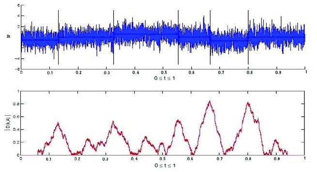
Figure 2.1: Above: Gaussian random variables simulated with constant variance and presenting changes in the mean. Below: Filtered derivative function D.

Nevertheless, we remark through the graph of the function $|D|$ that there are not only the "right hats" (surrounded in blue in Figure 2.2) which gives the right change points, but also false alarms (surrounded in green in Figure 2.2). Consequently, we have introduced another idea in order to keep just the right change points. This objective is reached by splitting the detection procedure into two successive steps: In Step 1, we detect potential change points as local maxima of the filtered derivative function. In Step 2, we test wether a potential change point is a false alarm or not. Both steps use estimation of the p-value of existence of change point.

The construction of two different statistical tests and the computation of p-values is detailed below.

Step 1: Detection of the potential change points

In order to detect the potential change points, we test the null hypothesis $(H_{0})$ of no change in the parameter $\theta$

$$(H_{0}):\ \theta_{1}=\theta_{2}=\cdots=\theta_{n-1}=\theta_{n}$$

against the alternative hypothesis $(H_{1})$ indicating the existence of one or more than one changes

$$(H_{1}):\ \text{There is an integer }K\in\mathbb{N}^{*}\text{ and }0=\tau_{0}<\tau_{1}<\dots<\tau_{K}<\tau_{K+1}=n\text{ such that }$$

$$\theta_{1}=\cdots=\theta_{\tau_{1}}\neq\theta_{\tau_{1}+1}=\cdots=\theta_{\tau_{2}}\cdots\neq\theta_{\tau_{K}+1}=\cdots=\theta_{\tau_{K+1}}.$$

where $\theta_{i}$ is the value of the parameter $\theta$ for $1\leq i\leq n$.

In Antoch and Hušková (1994) or Bertrand (2000), potential change points are selected as times $\tau_{k}$ corresponding to local maxima of the absolute value of the filtered derivative $|D(\tau_{k},A)|$, when moreover this last quantity exceeds a given threshold $\lambda$. However, the efficiency of the approach is strongly linked to the choice of the threshold $\lambda$. Therefore, in this work, we have a slightly different approach: we fix a probability of type I error at level $p_{1}^{*}$, and we determine the corresponding critical value $C_{1}$ given by

$$\mathbb{P}\left(\max_{k\in[A:n-A]}|D(k,A)|>C_{1}|\ H_{0}\text{ is true}\right)=p_{1}^{*}.$$

Of course, such a probability is usually not available, so that we only have the asymptotic distribution of the maximum of $|D|$, which will be the main part of Section 3 and Section 4. Then, roughly speaking, we select as potential change points, local maxima for which $\displaystyle|D(\tau_{k},A)|>C_{1}$.

By doing so, the p-value $p_{1}^{*}$ appears as an hyper parameter. The second hyper parameter is the window size $A$. As pointed out in Antoch and Hušková (1994); Bertrand (2000), Filtered Derivative method works under the implicit assumption that the minimal distance between two successive change points is greater than $2A$. An adaptive and automatic choice of $A$ is an open and particularly relevant question, but there is no such result in the litterature. Thus, we need some a priori knowledge on the minimal length between two successive changes.

More formally, we have the following algorithm:
 
Step 1 of the algorithm

1. Choice of the hyper parameters

   • Choice of the window size $A$ from information of the practitioners.

   • Choice of $p_{1}^{*}$:
     First we fix the significance level of type I error at $p_{1}^{*}$. Then, the theoretic expression of type I error, given in Section 3 and Section 4, fixes the value of the threshold $C_{1}$.
     The list of potential change points, which contains right change points as well as false ones, can be too large. So the level of significance for Step 1 can be chosen large, i.e. $p_{1}^{*}=5\%\text{ or }10\%$.

2. Computation of the filtered derivative function

   • The memory complexity results from the recording of the filtered derivative sequence $\displaystyle\left(D(k,A)\right)_{A\leq k\leq n-A}$. Clearly, we need a second buffer of size $(n-2A)$. Thus the memory complexity is of order $n$. On the other hand, filtered derivative function can be calculated by recurrence, see $\eqref{rec1}$ or $\eqref{rec2}$ and $\eqref{def:hat:b}$. These recurrence formulas induce time complexity of order $n\times\mathcal{C}$ where $\mathcal{C}$ is the time complexity of an iteration. For instance, in $\eqref{rec1}$ we have $\mathcal{C}\simeq 4\,additions$, in $\eqref{rec2}$ we have $\mathcal{C}\simeq 5\,additions+5\,multiplications+1\,division$, and in $\eqref{def:hat:b}$, $\mathcal{C}\simeq 3\,additions+1\,division$.

3. Determination of the potential change points

   • Initialization: 
     Set counter of potential change point $k=0$ and $\widetilde{\tau}_{k}=\operatorname*{arg\,max}_{k\in[A,n-A]}|D(k,A)|$.

   • While ($\displaystyle|D(\widetilde{\tau}_{k},A)|>C_{1}$) do

     • $k=k+1$

     • $D(k,A)=0$ for all $k\in(\widetilde{\tau}_{k}-A,\widetilde{\tau}_{k}+A)$.

     • $\widetilde{\tau}_{k}=\operatorname*{arg\,max}_{k\in[A,n-A]}|D(k,A)|$

     We increment the change point counter and we set the values of the function $D$ to zero because the width of the hat is equal to $2A$.

   • Finally, we sort the vector $\displaystyle\left(\widetilde{\tau}_{1},\ldots,\widetilde{\tau}_{K_{\max}}\right)$ in increasing order. The integer $K_{\max}$ represents the number of potential change points detected at the end of the Step 1. By construction, we have $K_{\max}\leq\lfloor n/A\rfloor-2$, where $\lfloor x\rfloor$ corresponds to the integer part of $x$.

End of the Step 1 of the algorithm

Figure 2.2 below provides an example: The family of potential change points contains the right change points (surrounded in blue in Figure 2.2) as well as false alarms (surrounded in green in Figure 2.2).

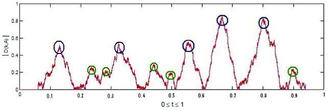
Figure 2.2: Detection of potential change points

Step 2: Removing false detection

The list of potential change points $\displaystyle\left(\widetilde{\tau}_{1},\ldots,\widetilde{\tau}_{K_{\max}}\right)$ obtained at step 1 contains right change points but also false detections. In the second step a test is carried out to remove the false detection from the list of change points found at step 1. By doing so, we obtain a subset $\displaystyle\left(\widehat{\tau}_{1},\ldots,\widehat{\tau}_{\widehat{K}}\right)$ of the first list.

More precisely, for all potential change point $\widetilde{\tau}_{k}$, we test wether the parameter is the same on the two successive intervals $(\widetilde{\tau}_{k-1}+1,\widetilde{\tau}_{k})$ and $(\widetilde{\tau}_{k}+1,\widetilde{\tau}_{k+1})$, or not. Formally, for all $1\leq k\leq K_{\max}$, we apply the following hypothesis testing

$$(H_{0,k}):\theta_{k}=\theta_{k+1} (H_{1,k}):\theta_{k}\neq\theta_{k+1}$$ versus

where $\theta_{k}$ is the value of $\theta$ supposed to be constant on the segment $(\widetilde{\tau}_{k-1}+1,\widetilde{\tau}_{k})$. By using this second test, we calculate new p-values $\displaystyle(\widetilde{p}_{1},\ldots,\widetilde{p}_{K_{\max}})$ associated respectively to each potential change points $\displaystyle(\widetilde{\tau}_{1},\ldots,\widetilde{\tau}_{K_{\max}})$. Then, we only keep the change points which have a p-value smaller than a critical level denoted $p_{2}^{*}$. Step 2 must be much more selective with a significance level $p_{2}^{*}=10^{-3}\text{ or }10^{-4}$. Consequently, Step 2 permits us to remove most of false detections, and so to deduce an estimator of the piecewise constant map $t\mapsto\theta(t)$, see Figure 2.3 below.

Remark 2.1

We note that $\widetilde{\tau}_{k}$, for $1\leq k\leq K_{\max}$, is a random variable. So that at first sight, the average value of the parameter $\theta$ on the interval $(\widetilde{\tau}_{k-1}+1,\widetilde{\tau}_{k})$ may also be a random variable. However, Bertrand (2000) has showed that, with probability converging to 1, the right change point is in $(\widetilde{\tau}_{k}+\epsilon_{k},\widetilde{\tau}_{k}-\epsilon_{k})$, where $\epsilon_{k}$ is a given bounded real number. For the detection of change in the mean in a series of independent Gaussian random variables, Bertrand (2000, Theorem 3.1, p.255) has proved that $\epsilon_{k}=5(\sigma/\delta_{k})^{2}+1$ where $\delta_{k}$ represents the size of change in the mean at $\tau_{k}$. This result can be easily generalized to a series of independent non Gaussian random variables with finite second moment. Therefore, on a set $\Omega_{n}$ with $\mathbb{P}(\Omega_{n})\rightarrow 1$ as $n\rightarrow\infty$, the average value of $\theta$ on the segment $(\widetilde{\tau}_{k}+\epsilon_{k},\widetilde{\tau}_{k}-\epsilon_{k})$ becomes not random and actually is equal to $\theta_{k}$.

The time and memory complexity of this second step of the algorithm is still $\mathcal{O}(n)$ because we only need to compute and to stock $(K_{\max}+1)$ estimators of parameter $\theta$ which are successively compared two by two in order to eliminate false alarms.

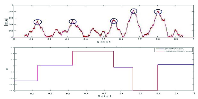
Figure 2.3: Above: Detection of right change points. Below: Theoretical value of the piecewise-constant map $t\mapsto\mu_{t}$ (black), and its estimators given by PLSC method (blue) and FDp-V method (red).

To sum up, FDp-V method is a two step procedure, in which the filtered derivative method is applied first and then a second test is carried out to remove the false detection from the list of change points found in Step 1. The first step has both time and memory complexity of order $\mathcal{O}(n)$. At the second step, the number of selected potential change points is smaller. As a consequence, both time and memory complexity of Step 2 are still of order $\mathcal{O}(n)$.

Let us finish the presentation of the FDpV algorithm by the following remark: in this paper we will restrict ourselves to the detection of change points of a one dimensional parameter, such as mean, variance, slope and intercept of linear regression. However, our algorithm still works in any finite dimension parameter space. Indeed, for each parameter, we can compute the corresponding filtered derivative sequence and its asymptotic distribution and then compare it to the corresponding type I errors $p^{*}_{1}$ and $p^{*}_{2}$.

3 THEORETICAL RESULTS

In this section, we present theoretical results of the FDp-V method for detecting changes on the mean and on the variance. The two following subsections give the asymptotic distribution of the filtered derivative used for the detection of potential change points. Then, Subsection 3.3 provides formulae for computing the p-values during Step 2 in order to eliminate false alarms.

3.1 Change in the mean

Let $\displaystyle(X_{i})_{i=1,\dots,n}$ be a sequence of independent r.v. with mean $\mu_{i}$ and a known variance $\sigma^{2}$. We assume that the map $i\mapsto\mu_{i}$ is piecewise constant, i.e. there exists a configuration $0=\tau_{0}<\tau_{1}<\dots<\tau_{K}<\tau_{K+1}=n$ such that $\mathbb{E}(X_{i})=\mu_{k}$ for $\tau_{k}\leq i<\tau_{k+1}$. The integer $K$ corresponds to the number of changes. However, in any real life situation, the number of abrupt changes $K$ is unknown, leading to a problem of model selection, see e.g. Birgé and Massart (2007).
Filtered Derivative method applied to the mean is based on the difference between the empirical mean computed on two sliding windows respectively at the right and at the left of the index $k$, both of size $A$, see Antoch and Hušková (1994); Basseville and Nikiforov (1993). This difference corresponds to a sequence $(D_{1}(k,A))_{A\leq k\leq n-A}$ defined by

$$D_{1}(k,A) = \hat{\mu}(k,A)-\hat{\mu}(k-A,A)$$ (3.1)

where $\hat{\mu}(k,A)=\frac{1}{A}\sum_{j=k+1}^{k+A}X_{j}$ is the empirical mean of $X$ on the (sliding) box $[k+1,\,k+A]$. These quantities can easily be calculated by recurrence with complexity $\mathcal{O}(n)$. It suffices to remark that

$$A\times D_{1}(k+1,A)=A\times D_{1}(k,A)+X_{k+A+1}-2X_{k}+X_{k-A+1}.$$ (3.2)

First we give in Theorem 3.1 the asymptotic behaviour of the maximum of $|D_{1}|$ under null hypothesis of no change in the mean and with size of the sliding windows tending to infinity at a certain rate. In the sequel, we denote by $A_{n}$ the size of the sliding windows and we will always suppose that

$$\lim\limits_{\begin{subarray}{c}n\to+\infty\end{subarray}}\frac{A_{n}}{n}=0\text{ and }\lim\limits_{\begin{subarray}{c}n\to+\infty\end{subarray}}\frac{(\log n)^{2}}{A_{n}}=0.$$ (3.3)

Theorem 3.1 (Change point in the mean with known variance)

Let $\displaystyle(X_{i})_{i=1,\dots,n}$ be a sequence of independent identically distributed random variables with mean $\mu$, variance $\sigma^{2}$ and assume that one of the following assumptions is satisfied

$\mathbf{(\mathcal{A}_{1})}$

$\ X_{1}\sim\mathcal{N}(\mu,\sigma^{2}).$

$\mathbf{(\mathcal{A}_{2})}$

$\exists\,t>0\text{ such as }\ \mathbb{E}[\exp(tX_{1})]<+\infty\text{, and }\displaystyle\lim\limits_{\begin{subarray}{c}n\to+\infty\end{subarray}}\frac{(\log n)^{3}}{A_{n}}=0.$

$\mathbf{(\mathcal{A}_{3})}$

$\exists\,p>2\text{ such as }\mathbb{E}[|X_{1}|^{p}]<+\infty\text{, and }\displaystyle\lim\limits_{\begin{subarray}{c}n\to+\infty\end{subarray}}\frac{n^{2/p}\log n}{A_{n}}=0.$

Let $D_{1}$ be defined by (3.1). Then under the null hypothesis

$$\lim\limits_{\begin{subarray}{c}n\to+\infty\end{subarray}}\mathbb{P}\left(\max_{k\in[A_{n}:n-A_{n}]}|D_{1}(k,A_{n})|\leq\frac{\sigma}{\sqrt{A_{n}}}c_{n}(x)\right)=\exp(-2e^{-x}),$$ (3.4)

$$c_{n}(x)=c\left(\frac{n}{A_{n}}-1,x\right)$$ (3.5)

$$c(y,x)=\frac{1}{\sqrt{2\log y}}\left(x+2\log y+\frac{1}{2}\log\log y-\frac{1}{2}\log\pi\right).$$ (3.6)

$\square$

A similar version of Theorem 3.1 was first proved by Chen (1988), via the strong invariance principle, in order to detect changes in the mean. Later, Steinebach and Eastwood (1995) have studied the same results for the detection of changes in the intensity of the renewal counting processes, and have improved them by giving another rate for the size of the sliding window under assumptions $\mathbf{(\mathcal{A}_{2})}$ and $\mathbf{(\mathcal{A}_{3})}$. The reader is also referred to the book of Révész (1990) for a good summary about the increments on partial sums.

Furthermore, for a known change point $\tau_{k}$, the law of the random variable $D_{1}(\tau_{k},A_{n})$ defined by $\eqref{def:D1}$ is known. Therefore, the probability to detect a known change point in the mean is described in the following remark.

Remark 3.1 (Probability to detect known change point in the mean)

Let $\tau_{k}$ be a known change point in the mean of size $\delta_{k}:=|\mu_{\tau_{k}}-\mu_{\tau_{k}+1}|$. Then, under assumption $\mathbf{(\mathcal{A}_{1})}$, the probability to detect it is given by

$$\mathbb{P}\left(|D_{1}(\tau_{k},A_{n})|\geq C_{1}\right)=1-\phi\left(\frac{(C_{1}-\delta_{k})\sqrt{A_{n}}}{\sqrt{2}\sigma}\right)+\phi\left(\frac{(-C_{1}-\delta_{k})\sqrt{A_{n}}}{\sqrt{2}\sigma}\right),$$ (3.7)

and under assumptions $\mathbf{(\mathcal{A}_{2})}$ and $\mathbf{(\mathcal{A}_{3})}$, we have the following asymptotic probability

$$\lim\limits_{\begin{subarray}{c}n\to+\infty\end{subarray}}\mathbb{P}\left(\sqrt{A_{n}}|D_{1}(\tau_{k},A_{n})-\delta_{k}|\geq C_{1}\right)=2\phi\left(\frac{-C_{1}}{\sqrt{2}\sigma}\right)$$ (3.8)

where $C_{1}$ is the threshold fixed in Step 1 and $\phi$ is the standard normal distribution. The proof can be deduced from $\displaystyle D_{1}(\tau_{k},A_{n})=\delta_{k}+\frac{\sqrt{2}\sigma}{\sqrt{A_{n}}}Z$ where $Z$ is the standard normal r.v.

In applications, the variance $\sigma^{2}$ is unknown. For this reason we may replace it by its empirical estimator, $\widehat{\sigma}_{n}^{2}$. But, in order to keep the same result as in Theorem 3.1, the estimator $\widehat{\sigma}_{n}^{2}$ has to verify a certain condition given by the following theorem.

Theorem 3.2 (Change point in the mean with unknown variance)

We apply to the same notations and the same assumptions as in Theorem 3.1. Moreover, we assume that $\widehat{\sigma}_{n}$ is an estimator of $\sigma$ satisfying

$$\lim\limits_{\begin{subarray}{c}n\to+\infty\end{subarray}}|\sigma-\widehat{\sigma}_{n}|\log n\stackrel{{\scriptstyle P}}{{=}}0,$$ (3.9)

where the sign $\stackrel{{\scriptstyle P}}{{=}}$ means convergence in probability. Then, under the null hypothesis,

$$\lim\limits_{\begin{subarray}{c}n\to+\infty\end{subarray}}\mathbb{P}\left(\max_{k\in[A_{n}:n-A_{n}]}|D_{1}(k,A_{n})|\leq\frac{\widehat{\sigma}_{n}}{\sqrt{A_{n}}}c_{n}(x)\right)=\exp(-2e^{-x}).$$ (3.10)

$\square$

Remark that condition (3.9) is not really restrictive, indeed as soon as $\widehat{\sigma}^{2}_{n}$ satisfies a CLT, the condition is verified. For example, with the usual empirical variance estimator, a fourth order moment (of $X$) is sufficient.

3.2 Change in the variance

Now, we consider the case where we have a set of observations $\displaystyle(X_{i})_{i=1,\dots,n}$ and we wish to know whether their variance has changed at an unknown time. If $\mu$ is known, then the problem is very simple. Testing $(H_{0})$ against $(H_{1})$ means that we are looking for a change in the mean of the sequence $\displaystyle\left((X_{i}-\mu)^{2}\right)_{i=1,\dots,n}$.
Filtered Derivative method applied to the variance is based on the difference between the empirical variance computed on two sliding windows respectively at the right and at the left of the index $k$, both of size $A_{n}$ which satisfy condition $\eqref{An}$. This difference is in fact a sequence of random variables denoted by $(D_{2}(k,A_{n}))_{A_{n}\leq k\leq n-A_{n}}$ and defined as follows

$$D_{2}(k,A_{n}) = \hat{\sigma}^{2}(k,A_{n})-\hat{\sigma}^{2}(k-A_{n},A_{n})$$ (3.11)

where

$$\hat{\sigma}^{2}(k,A_{n}) = \frac{1}{A_{n}}\sum_{j=k+1}^{k+A_{n}}(X_{j}-\mu)^{2}$$

denotes the empirical variance of $X$ on the box $[k+1,k+A_{n}]$. By using Theorem 3.1, we can deduce the asymptotic distribution of the maximum of $|D_{2}|$ under null hypothesis $(H_{0})$. This gives straightforwardly the following corollary:

Corollary 3.1 (Change point in the variance with known mean)

Let $\displaystyle(X_{i})_{i=1,\dots,n}$ be a sequence of independent identically distributed random variables with mean $\mu$ and assume that one of the following assumptions is satisfied

$\mathbf{(\mathcal{A}_{4})}$

$\exists\,t>0\text{ such as }\ \mathbb{E}[\exp(t(X_{1}-\mu)^{2})]<+\infty\text{, and }\displaystyle\lim\limits_{\begin{subarray}{c}n\to+\infty\end{subarray}}\frac{(\log n)^{3}}{A_{n}}=0.$

$\mathbf{(\mathcal{A}_{5})}$

$\exists\,p>2\text{ such as }\ \mathbb{E}\left[|X_{1}-\mu|^{2p}\right]<+\infty\text{, and }\displaystyle\lim\limits_{\begin{subarray}{c}n\to+\infty\end{subarray}}\frac{n^{2/p}\log n}{A_{n}}=0.$

Let $D_{2}$ be defined by $\eqref{def:D2}$ and $\nu^{2}=\mbox{Var}\left[(X_{1}-\mu)^{2}\right]$. Then, under the null hypothesis,

$$\lim\limits_{\begin{subarray}{c}n\to+\infty\end{subarray}}\mathbb{P}\left(\max_{k\in[A_{n}:n-A_{n}]}|D_{2}(k,A_{n})|\leq\frac{\nu}{\sqrt{A_{n}}}c_{n}(x)\right)=\exp(-2e^{-x}),$$ (3.12)

where $c_{n}(.)$ is defined by $\eqref{cnx}$. $\square$

In practical situations we rarely know the value of the constant mean. However, $\hat{\mu}(k,A_{n})$ is a consistent estimator on the box $[k+1,\,k+A_{n}]$ for the mean $\mu$ under both null hypothesis $(H_{0})$ and alternative hypothesis $(H_{1})$. Thus, in the definition of the sequence $D_{2}$, $\mu$ can be replaced by its estimator $\hat{\mu}(k,A_{n})$ on the box $[k+1,\,k+A_{n}]$. To be precise, let

$$\widehat{D}_{2}(k,A_{n}) = \widetilde{\sigma}(k,A_{n})-\widetilde{\sigma}(k-A_{n},A_{n}),$$ (3.13)

where

$$\widetilde{\sigma}(k,A_{n}) = \frac{1}{A_{n}}\sum_{j=k+1}^{k+A_{n}}(X_{j}-\hat{\mu}(k,A_{n}))^{2}$$

denotes the empirical variance of $X$ on the sliding box $[k+1,\,k+A_{n}]$ with unknown mean. So, in order to obtain the same asymptotic distribution as the one obtained in Corollary 3.1, we must add extra conditions on the estimators $\hat{\mu}(k,A_{n})$. These new conditions are given in the next corollary.

Corollary 3.2 (Change point in the variance with unknown mean)

With the notations and assumptions of Corollary 3.1, we suppose moreover that

$$\lim\limits_{\begin{subarray}{c}n\to+\infty\end{subarray}}\max_{0\leq k\leq n-A_{n}}|\mu-\hat{\mu}(k,A_{n})|\left(A_{n}\log n\right)^{\frac{1}{4}}\stackrel{{\scriptstyle a.s}}{{=}}0$$ (3.14)

where the sign $\stackrel{{\scriptstyle a.s}}{{=}}$ means almost surely convergence. Then under the null hypothesis

$$\lim\limits_{\begin{subarray}{c}n\to+\infty\end{subarray}}\mathbb{P}\left(\max_{k\in[A_{n}:n-A_{n}]}|\widehat{D}_{2}(k,A_{n})|\leq\frac{\nu}{\sqrt{A_{n}}}c_{n}(x)\right)=\exp(-2e^{-x}).$$ (3.15)

$\square$

Let us remark that (3.14) is not a very stringent condition.

3.3 Step 2: calculus of p-values for changes on the mean and changes on the variance

In this subsection, we recall p-value formula associated with the second test in order to remove false alarms. Let us stress that the only novelty of this subsection is the idea to divide the detection of abrupt change into two steps, see section 3. Since the r.v. $X_{i}$ are independent, the calculus of p-value relies on well known results that can be found in any statistical textbook.

First, consider the Gaussian case and let us introduce some notations: For $1\leq k\leq K_{\max}$, let $(X_{\widetilde{\tau}_{k-1}+1},\ldots,X_{\widetilde{\tau}_{k}})$ and $(X_{\widetilde{\tau}_{k}+1},\ldots,X_{\widetilde{\tau}_{k+1}})$ two successive samples of i.i.d. Gaussian random variables such that

$$X_{\widetilde{\tau}_{k-1}+1}\sim\mathcal{N}(\mu_{k},\sigma_{k}^{2}) X_{\widetilde{\tau}_{k}+1}\sim\mathcal{N}(\mu_{k+1},\sigma_{k+1}^{2}).$$ and

We can use Fisher’s F-statistic to determine the p-value of the existence of a change on the variance at time $\widetilde{\tau}_{k}$ under the null assumption (H0): $\displaystyle\sigma_{k}^{2}=\sigma_{k+1}^{2}$. Then, we can use Student statistic to determine the p-value of a change on the mean at time $\widetilde{\tau}_{k}$, that is under the null assumption (H0): $\displaystyle\mu_{k}=\mu_{k+1}$.

Second, consider the general case. Since $A_{n}\to\infty$ and by construction $\displaystyle\widetilde{\tau}_{k+1}-\widetilde{\tau}_{k}\geq A_{n}$, we can apply CLT as soon as the r.v. $X_{i}$ satisfy Lindeberg condition. Thus, the empirical mean and the empirical variance converge to the corresponding ones in the Gaussian case. Eventually, if one of the assumptions $(\mathcal{A}_{i})$ for $i=1$, $2$ or $3$, then we can still apply Fisher and Student statistics to compute the p-value.

4 LINEAR REGRESSION

In this Section, we consider linear regression model:

$$Y_{i} = aX_{i}+b+e_{i},\text{ for }1\leq i\leq n,$$ (4.1)

where the terms $\left(e_{i}\right)_{i=1,\dots,n}$ are independent and identically distributed Gaussian random errors with zero-mean and variance $\sigma^{2}$ and, to simplify, $\left(X_{i}\right)_{i=1,\dots,n}$ are equidistant time points given by

$$X_{i}=i\Delta \quad\mathrm{with}\quad \Delta>0.$$ (4.2)

Our aim is to detect change points on the parameters $(a,b)$ of the linear model. As the Filtered Derivative is a local method, and to simplify notations, we will restrict ourselves here to one change point.

The two following subsections give the result for detection of potential change points on the slope and on the intercept. Subsection 4.3 provides formulas for calculating the p-values during Step 2.

4.1 Change in the slope

In this subsection, we are concerned with detection of change points in the slope $a$ when the intercept remains constant.

Filtered Derivative method applied to the slope is based on the differences between estimated values of the slope $a$ computed on two sliding windows at the right and at the left of the index $k$, both of size $A_{n}$. These differences, for $k\in[A_{n},n-A_{n}]$, form a sequence of random variables, given by

$$D_{3}(k,A_{n}) = \hat{a}(k,A_{n})-\hat{a}(k-A_{n},A_{n})$$ (4.3)

where

$$\hat{a}(k,A_{n})=\left[A\sum_{j=k+1}^{k+A}X_{j}Y_{j}-\sum_{j=k+1}^{k+A}X_{j}\sum_{j=k+1}^{k+A}Y_{j}\right]\,\left[A\sum_{j=k+1}^{k+A}X_{j}^{2}-\left(\sum_{j=k+1}^{k+A}X_{j}\right)^{2}\right]^{-1},$$ (4.4)

is the estimator of the slope $a$ on the (sliding) box $[k+1,\,k+A_{n}]$. Let us stress that these quantities can be calculated by recurrence with complexity $\mathcal{O}(n)$.
Our first result gives the asymptotic distribution of the maximum of $|D_{3}|$ under the null hypothesis of no change on the linear regression.

Theorem 4.1 (Change point in the slope)

Let $\left(X_{i}\right)_{i=1,\dots,n}$ and $\left(Y_{i}\right)_{i=1,\dots,n}$ be given by $\eqref{absXi}$ and $\eqref{ordYi}$ where $e_{i}$ is a family of i.i.d. mean zero Gaussian r.v. with variance $\sigma^{2}$. Let $D_{3}$ be defined by $\eqref{def:D3}$ and assume that $A_{n}$ satisfies condition $\eqref{An}$. Then under the null hypothesis

$$\lim\limits_{\begin{subarray}{c}n\to+\infty\end{subarray}}\mathbb{P}\left(\max_{k\in[A_{n}:n-A_{n}]}|D_{3}(k,A_{n})|\leq\frac{2\sqrt{6}\sigma}{\Delta\sqrt{A_{n}(A_{n}^{2}-1)}}d_{n}(x)\right)=\exp(-2e^{-x}),$$ (4.5)

with $d_{n}(x)=c\left(A_{n},x\right)$ and $c(.,.)$ is defined by $\eqref{cyx}$. $\square$

Moreover, for a given change point $\tau_{k}$, the law of the random variable $D_{3}(\tau_{k},A_{n})$ defined by $\eqref{def:D3}$ is known. Therefore, the probability to detect a known change point in the slope is specified in the following remark.

Remark 4.1 (Probability to detect known change point in the slope)

Let $\tau_{k}$ be a known change point in the slope of size $\delta_{a,k}:=|a_{\tau_{k}}-a_{\tau_{k}+1}|$. Then the probability to detect it is given by

$$\mathbb{P}\left(|D_{3}(\tau_{k},A_{n})|\geq C_{1}\right)=1-\phi\left(\frac{(C_{1}-\delta_{a,k})\Delta\sqrt{A_{n}(A_{n}^{2}-1)}}{2\sqrt{6}\sigma}\right)$$

$$\qquad\qquad\,\,\,+\phi\left(\frac{(-C_{1}-\delta_{a,k})\Delta\sqrt{A_{n}(A_{n}^{2}-1)}}{2\sqrt{6}\sigma}\right)$$ (4.6)

where $C_{1}$ is the threshold fixed in Step 1 and $\phi$ is the standard normal distribution. The proof is directly deduced from $\displaystyle D_{3}(\tau_{k},A_{n})=\delta_{a,k}+\frac{2\sqrt{6}\sigma}{\Delta\sqrt{A_{n}(A_{n}^{2}-1)}}Z$ where $Z$ is a standard normal random variable.

4.2 Change in the intercept

In this subsection, we focus on the detection of change points in the intercept with known slope $a$. To do this, we calculate the differences between estimators of the intercept $b$ computed on two sliding windows respectively at the right and at the left of the index $k$, both of size $A_{n}$. For $A_{n}\leq k\leq n-A_{n}$, these differences form a sequence of random variables given by

$$D_{4}(k,A_{n}) = \hat{b}(k,A_{n})-\hat{b}(k-A_{n},A_{n})$$ (4.7)

where

$$\hat{b}(k,A_{n}) = \frac{1}{A}\sum_{j=k+1}^{k+A}Y_{j}-a\times\frac{1}{A}\sum_{j=k+1}^{k+A}X_{j},$$ (4.8)

is the estimator of the intercept $b$ on the (sliding) box $[k+1,\,k+A_{n}]$. By applying Theorem 3.1, we get the asymptotic distribution of the maximum of $|D_{4}|$ under the null hypothesis of no change on the linear regression.

Corollary 4.1 (Change point in the intercept)

With the notations and assumptions of Theorem 4.1, we have under the null hypothesis

$$\lim\limits_{\begin{subarray}{c}n\to+\infty\end{subarray}}\mathbb{P}\left(\max_{k\in[A_{n}:n-A_{n}]}|D_{4}(k,A_{n})|\leq\frac{\sigma}{\sqrt{A_{n}}}c_{n}(x)\right)=\exp(-2e^{-x}),$$ (4.9)

where $c_{n}(.)$ is defined by $\eqref{cnx}$. $\square$

In addition, for a known change point $\tau_{k}$, the distribution of the random variable $D_{4}(\tau_{k},A_{n})$ defined by $\eqref{def:D4}$ is known. Therefore, the probability to detect a known change point in the intercept is given in the following remark.

Remark 4.2 (Probability to detect known change point in the intercept)

Let $\tau_{k}$ be a known change point in the intercept of size $\delta_{b,k}:=|b_{\tau_{k}}-b_{\tau_{k}+1}|$. Then the probability to detect it is given by

$$\mathbb{P}\left(|D_{4}(\tau_{k},A_{n})|\geq C_{1}\right)=1-\phi\left(\frac{(C_{1}-\delta_{b,k})\sqrt{A_{n}}}{\sqrt{2}\sigma}\right)+\phi\left(\frac{(-C_{1}-\delta_{b,k})\sqrt{A_{n}}}{\sqrt{2}\sigma}\right)$$ (4.10)

where $C_{1}$ is the threshold fixed in Step 1 and $\phi$ is the standard normal distribution. The proof may be easily deduced from $\displaystyle D_{4}(\tau_{k},A_{n})=\delta_{b,k}+\frac{\sqrt{2}\sigma}{\sqrt{A_{n}}}Z$ where $Z$ is a standard normal random variable.

In real applications the slope is often unknown. In this case, we replace it in $\eqref{def:D4}$ by its empirical estimator $\widehat{a}_{n}$. This leads to the definition

$$\widehat{D}_{4}(k,A_{n}) = \widetilde{b}(k,A_{n})-\widetilde{b}(k-A_{n},A_{n})$$ (4.11)

where

$$\widetilde{b}(k,A_{n})=\frac{1}{A}\sum_{j=k+1}^{k+A}Y_{j}-\widehat{a}_{n}\times\frac{1}{A}\sum_{j=k+1}^{k+A}X_{j},$$

is the estimator of the intercept $b$ on the (sliding) box $[k+1,\,k+A_{n}]$ with unknown slope.
Naturally, we must assume that the estimator of the slope satisfy a certain convergence condition which is given in the following corollary.

Corollary 4.2 (Change point in the intercept with unknown slope)

Under the same notations and the same assumptions than in Corollary 4.1. Moreover, we assume that the estimator $\hat{a}_{n}$ of $a$ satisfies the following condition

$$\lim\limits_{\begin{subarray}{c}n\to+\infty\end{subarray}}|a-\hat{a}_{n}|A_{n}^{\frac{3}{2}}\Delta_{n}\sqrt{\log n}\stackrel{{\scriptstyle a.s}}{{=}}0$$ (4.12)

where the sign $\stackrel{{\scriptstyle a.s}}{{=}}$ means almost surely convergence. Then under the null hypothesis

$$\lim\limits_{\begin{subarray}{c}n\to+\infty\end{subarray}}\mathbb{P}\left(\max_{k\in[A_{n}:n-A_{n}]}|\widehat{D}_{4}(k,A_{n})|\leq\frac{\sigma}{\sqrt{A_{n}}}c_{n}(x)\right)=\exp(-2e^{-x}).$$ (4.13)

$\square$

4.3 Step 2: calculus of p-values

Let us give here p-value formulae associated to Step 2 in linear regression model $\eqref{absXi}$ and $\eqref{ordYi}$. More precisely, we are concerned with detection of right change points on the slope or intercept. We recall that Step 2 of FDp-V method has been introduced in order to eliminate false alarms. Indeed, at Step 1, a time $X_{\widetilde{\tau}_{k}}$ has been selected as a potential change point. At Step 2, we test whether the slopes and intercepts of two data sets at left and right of the potential change point $X_{\widetilde{\tau}_{k}}$ are significantly different or not, and we measure this by the corresponding p-value.

Before going further, let us introduce some notations. For $1\leq k\leq K_{\max}$, let $\mathcal{R}_{k}=\left((X_{\widetilde{\tau}_{k-1}+1},Y_{\widetilde{\tau}_{k-1}+1}),\ldots,(X_{\widetilde{\tau}_{k}},Y_{\widetilde{\tau}_{k}})\right)$ and $\mathcal{R}_{k+1}=\left((X_{\widetilde{\tau}_{k}+1},Y_{\widetilde{\tau}_{k}+1}),\ldots,(X_{\widetilde{\tau}_{k+1}},Y_{\widetilde{\tau}_{k+1}})\right)$ two successive samples of observations such that the relationship between variables $X$ and $Y$ is given by $\eqref{absXi}$ and $\eqref{ordYi}$, or more explicitly by

$$Y_{j} = a_{k}X_{j}+b_{k}+e_{j}\qquad\qquad\text{ for }\,\widetilde{\tau}_{k-1}+1\leq j\leq\widetilde{\tau}_{k}.$$

By using definition of the error terms,we can easily see that slope estimator $\widehat{a}_{k}$ and intercept estimator $\widehat{b}_{k}$ have Gaussian distribution given by

$$\widehat{a}_{k} \sim \mathcal{N}\left(a_{k},\sigma^{2}_{a_{k}}\right)\text{ with }\frac{\sigma_{a_{k}}^{2}}{\sigma^{2}}=\left(\sum_{j=\widetilde{\tau}_{k-1}+1}^{\widetilde{\tau}_{k}}(X_{j}-\overline{X}_{k})^{2}\right)^{-1},$$

$$\widehat{b}_{k} \sim \mathcal{N}\left(b_{k},\sigma^{2}_{b_{k}}\right)\text{ with }\frac{\sigma_{b_{k}}^{2}}{\sigma^{2}}=\frac{1}{n_{k}}+\overline{X}_{k}\left(\sum_{j=\widetilde{\tau}_{k-1}+1}^{\widetilde{\tau}_{k}}(X_{j}-\overline{X}_{k})^{2}\right)^{-1},$$

respectively, where $\overline{X}_{k}$ is the empirical mean of the sequence $\displaystyle\left(X_{\widetilde{\tau}_{k-1}+1},\ldots,X_{\widetilde{\tau}_{k}}\right)$. In the sequel, we denote by $\widehat{\sigma}_{a_{k}}^{2}$ and $\widehat{\sigma}_{b_{k}}^{2}$ the empirical variance of respectively the random variables $\widehat{a}_{k}$ and $\widehat{b}_{k}$.

Comparing slope

We want to test if the samples $\mathcal{R}_{k}$ and $\mathcal{R}_{k+1}$ present a change in slope or not.

$$\left(H_{0,k}^{a}\right):\ a_{k}=a_{k+1} \left(H_{1,k}^{a}\right):\ a_{k}\neq a_{k+1}.$$ against

Then, the p-value $\widetilde{p}_{k,a}$ associated to the potential change point $\widetilde{\tau}_{k}$ in order to eliminate false alarms for changes in slope is given by

$$\widetilde{p}_{k,a}=1-\phi_{a}\left(\frac{|\widehat{a}_{k}-\widehat{a}_{k+1}|}{\sqrt{\frac{\widehat{\sigma}^{2}_{a_{k}}}{n_{k}}+\frac{\widehat{\sigma}^{2}_{a_{k+1}}}{n_{k+1}}}}\right)$$

where $\phi_{a}$ is a Student T-distribution with $\upsilon_{a}$ degrees of freedom

$$\upsilon_{a}=N\left(\widehat{\sigma}^{2}_{a_{k}},\widehat{\sigma}^{2}_{a_{k+1}},n_{k},n_{k+1}\right)=\left\lfloor\frac{\left(\frac{\widehat{\sigma}^{2}_{a_{k}}}{n_{k}}+\frac{\widehat{\sigma}^{2}_{a_{k+1}}}{n_{k+1}}\right)^{2}}{\left(\frac{\widehat{\sigma}^{2}_{a_{k}}}{n_{k}\sqrt{n_{k}-1}}\right)^{2}+\left(\frac{\widehat{\sigma}^{2}_{a_{k+1}}}{n_{k+1}\sqrt{n_{k+1}-1}}\right)^{2}}\right\rfloor$$

and $\lfloor x\rfloor$ is the integer part of $x$.

Comparing intercept

We desire to study if the intercept before and after a detected change points $\tilde{\tau}_{k}$ are equal or not, i.e. if it is a real change point, resulting in testing

$$(H_{0,k}^{b})\ b_{k}=b_{k+1} (H_{1,k}^{b})\ b_{k}\neq b_{k+1}.$$ against

Then, the p-value $\widetilde{p}_{k,b}$ associated to the potential change point $\widetilde{\tau}_{k}$ in order to remove false alarms from the list of changes in intercept found in step 1, is given by

$$\widetilde{p}_{k,b}=1-\phi_{b}\left(\frac{|\widehat{b}_{k}-\widehat{b}_{k+1}|}{\sqrt{\frac{\widehat{\sigma}^{2}_{b_{k}}}{n_{k}}+\frac{\widehat{\sigma}^{2}_{b_{k+1}}}{n_{k+1}}}}\right)$$

where $\phi_{b}$ is a Student T-distribution with $\displaystyle\upsilon_{b}=N\left(\widehat{\sigma}^{2}_{b_{k}},\widehat{\sigma}^{2}_{b_{k+1}},n_{k},n_{k+1}\right)$ degrees of freedom.

5 NUMERICAL RESULTS

In this section, we apply FDpV and PLSC methods to detect abrupt changes in the mean of simulated Gaussian r.v and we compare the results obtained by both methods. Next, we use the FDpV for the detection of change points in the slope of linear regression model. Finally, we run the FDpV algorithm to the segmentation of heartbeat time series, and average daily volume drawn from the financial market.

5.1 A toy model: off-line detection of abrupt changes in the mean of independent Gaussian random variables with known variance

In the following subsection, we consider the elementary problem, namely: The off-line detection of multiple change points in the mean of simulated independent Gaussian r.v with known variance, and we numerically compare the efficiency of the different estimators given by the FDpV and the PLSC procedures.

Numerical simulation

To begin, for $n=5000$ we have simulated a sequence of Gaussian r.v $\left(X_{1},\ldots,X_{n}\right)$ with known variance $\sigma^{2}=1$ and mean $\mu_{i}=g(i/n)$ where $g$ is a piecewise-constant function with five change points, i.e. we have chosen a configuration $1=\tau_{0}<\tau_{1}<\dots<\tau_{K}<\tau_{K+1}=n$ with $K=5$ and such as $\mu_{i}=g(k)$ for $\tau_{k}\leq i<\tau_{k+1}$ . The size of the change point at $\tau_{k}$ specified by $\delta_{k}:=|\mu_{\tau_{k}}-\mu_{\tau_{k}+1}|$ are to be chosen in the intervalle $[0.5,1.25]$.
Then, we have computed the function $k\rightarrow|D_{1}(A,k)|$ with $A=300$, see Figure 2.1.
Both methods, namely Filtered Derivative with p-values, $p_{1}^{*}=0.05$ and $p_{2}^{*}=10^{-4}$, and Penalized Least Squares Criterion provide right results, see Figure 2.3. This example is plainly confirmed by Monte-Carlo simulations.

Monte-Carlo simulation

In this paragraph, we have made $M=1000$ simulations of independent copies of sequences of Gaussian r.v. $X_{1}^{(k)},\ldots,X_{n}^{(k)}$ with variance $\sigma^{2}=1$ and mean $\mu(i)=g(i/n)$, for $k=1,\dots,M$. On each sample, we apply the FDp-V algorithm and the PLSC method. We find the right number of changes in $98.1\%$ of all cases for the first method and in $97.9\%$ for the second one, see Figure 5.1.

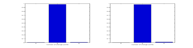
Figure 5.1: Distribution of the estimated number of change points $\widehat{K}$ for $M=1000$ realizations. Left: Using PLSC method. Right: Using Filtered Derivative method.

Then, we compute the mean square errors. There are two kinds of mean square errors:

• Mean Integrate Square Error: $\mathbb{E}\left(\frac{1}{n}\sum_{i=1}^{n}\left|\widehat{g}(i/n)-g(i/n)\right|^{2}\right)=\mathbb{E}\|\widehat{g}-g\|_{L^{2}([0,1])}^{2}$.The estimated function is obtained in two steps: first we estimate the configuration of change points $(\hat{\tau}_{k})_{k=1,\dots,\hat{K}}$, then we estimate the value of $\widehat{g}$ between two successive change points as the empirical mean.

• Square Error on Change Points: $\displaystyle\mathbb{E}\left(\sum_{k=1}^{K}\left|\widehat{\tau}_{k}-\tau_{k}\right|^{2}\right)$, in the case where we have found the right number of change points.

Table 1 gives the result of Monte Carlo simulation mean errors, and also the comparison between the mean time complexity and the mean memory complexity. We have written the two programs in Matlab and have runned it with computer system which has the following characteristics: 1.8GHz processor and $512$MB memory.

	Square Error on Change Points	Mean Integrated Squared Error
FDp-V method	$1.1840\times 10^{-4}$	$0.0107$
PLSC method	$1.2947\times 10^{-4}$	$0.0114$
	Memory allocation (in Megabytes)	CPU time (in second)
FDp-V method	$0.04$ MB	$0.005$ s
PLSC method	$200$ MB	$240$ s

Table 5.1: Errors and complexities given by FDp-V method and PLSC method.

Numerical conclusion

On the one hand, both methods have the same accuracy in terms of percentage of the right number of changes, and in terms of Square Error or Mean Integrate Square Error. On the other hand, the Filtered Derivative with p-Value is less expensive in terms of time complexity and memory complexity, see Table 5.1. Indeed, Penalized Least Squares Criterion algorithm needs 200 Megabytes of computer memory, while Filtered derivative method only needs $0.008\%$. This plainly confirms the difference of time and memory complexity, i.e. $\mathcal{O}(n^{2})$ versus $\mathcal{O}(n)$.

5.2 Off-line detection of changes in the slope of simple linear regression

In this subsection, we consider the problem of multiple change points detection in the slope of linear model corrupted by an additive Gaussian noise.
At first, for $n=1400$ we have simulated the sequences $X=\left(X_{1},\ldots,X_{n}\right)$ and $Y=\left(Y_{1},\ldots,Y_{n}\right)$ defined by $\eqref{absXi}$ and $\eqref{ordYi}$ with $\Delta=1$, $\sigma=30$ and $a_{i}=h(i)$ where $h$ is a piecewise-constant function with four change points, i.e. we have chosen a configuration $1=\tau_{0}<\tau_{1}<\dots<\tau_{K}<\tau_{K+1}=n$ with $K=4$ and such as $a_{i}=h(k)$ for $\tau_{k}\leq i<\tau_{k+1}$ . On the one hand, we have considered large change points in the slope such as $\nu_{k}\in[3,5]$ where $\nu_{k}:=|a_{\tau_{k}}-a_{\tau_{k}+1}|$ represents the size of the change point at $\tau_{k}$. On the other hand, we have chosen smaller change points such as $\nu_{k}\in[0.75,1]$. Next, we have plot $X$ versus $Y$, see the scatter plots 5.2 and 5.5. Then, to detect the change points in the slope of these simulated data, we have computed the function $k\mapsto|D_{3}(k,A)|$ with $A=100$, see Figures 5.3 and 5.6.
Finally, by applying FDp-V procedure with p-values $p_{1}^{*}=0.05$ and $p_{2}^{*}=10^{-10}$, we obtain a right localization of the change points and so a right estimation of the piecewise-constant function $h$, see Figures 5.4 and 5.7.

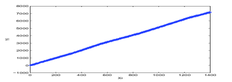
Figure 5.2: Case 1: Scatter plot of the simulated data $(X_{i},Y_{i})$ for $1\leq i\leq n$.

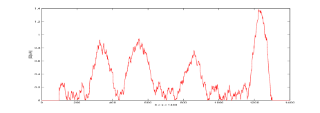
Figure 5.3: Case 1: The hat function |$D_{3}$|.

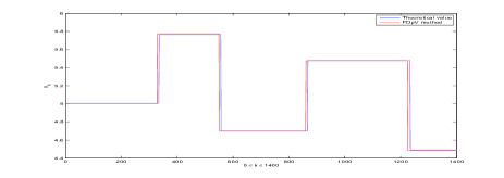
Figure 5.4: Case 1: Theoretical value of the piecewise-constant function $h$ (blue), and its estimator given by FDp-V method (red).

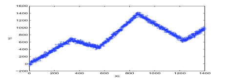
Figure 5.5: Case 2: Scatter plot of the simulated data $(X_{i},Y_{i})$ for $1\leq i\leq n$.

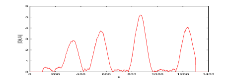
Figure 5.6: Case 2: The hat function |$D_{3}$|.

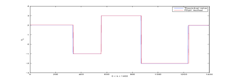
Figure 5.7: Case 2: Theoretical value of the piecewise-constant function $h$ (blue), and its estimator given by FDp-V method (red).

5.3 Application to real data

In this subsection, we apply our algorithm to detect change points in the mean of two real samples: the first one is concerned with health and wellbeing, and the second one with finance. Our main purpose here is to show that our estimation procedure is sufficiently robust to consider non-independent time series, that we will study theoretically in a subsequent paper. We moreover provide an analysis of the obtained results.

An Application to Change Point Detection of Heartbeat Time Series

In this paragraph, we give examples of application of FDp-V method to heartbeat time series analysis. Electrocardiogram (ECG) has been processed from a long time since the implementation of monitoring by Holter in the fifties. We consider here the RR interval, which provides an accurate measure of the length of each single heartbeat and corresponds to the instantaneous speed of the heart engine, see Task force of the European Soc. Cardiology and the North American Society of Pacing and Electrophysiology (1996). From the beginning of 21st century, the size reduction of the measurement devices allows to record heartbeat time series for healthy people in ecological situations throughout long periods of time: Marathon runners, individuals daily (24 hours) records, etc. We then obtain large data sets of more than 40.000 observations, resp. 100,000 observations, that address change detection of heart rate.

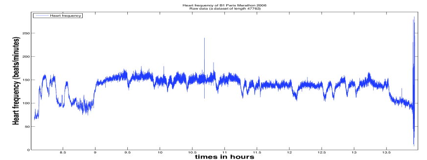
Figure 5.8: Raw heart rate time series of a marathon runner

In Figure 5.8, Figure 5.9 and Figure 5.10, we give two examples: In Figure 5.8, the hearbeat time series correspond to a marathon runner. This raw dataset has been recorded by the team UBIAE (U. 902, INSERM and Évry Génopole) during Paris Marathon 2006. This work is part of the project "Physiostat" (2009-2011) which is supported by device grants from Digitéo and Région Île-de- France. The hearbeat time series used in Figure 5.10 corresponds to a day in the life of a shift worker. It has been kindly given by Gil Boudet and Professor Alain Chamoux (Occupational Safety service of Clermont Hospital).

Data are then been preprocessed by using the "tachogram cleaning" algorithm developed by Nadia Khalfa and P.R. Bertrand at INRIA Saclay in 2009. "Tachogram cleaning" cancelled aberrant data, based on physiological considerations rather than statistical procedure. Next, segmentations of the cleaned heart beat time series can be obtained by using the software "In Vivo Tachogram Analysis (InViTA)" developed by P.R. Bertrand at INRIA Saclay in 2010, see Figure 5.9 and Figure  5.10 below.

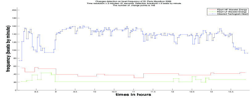
Figure 5.9: Segmentation of heartbeat time series of a marathon runner. Blue: Heart rate segmented by FDpV. Red: Low Frequency wavelet energy segmented by FDpV. Green: High Frequency wavelet energy segmented by FDpV

Let us comment Fig. 5.9 and Fig. 5.10: first, for readability, we give the times in hours and minutes in abscissa and the heart rate rather than RR-interval in ordinate. We recall the equation: $\quad HeartRate=60/RR\leavevmode\nobreak\ Interval\quad$ and we stress that all the computations are done on RR-interval. Secondly, in Figure 5.9, we notice beginning and end of the marathon race, but also training before the race, and small breaks during the race. The same FDpV compression technology has been applied to wavelet energy corresponding to High Frequency, resp. Low Frequency band. Energy into these two frequencies bands is interpreted by cardiologists as corresponding to heart rate regulation by sympathetic and ortho-sympathetic systems. We refer to Ayache and Bertrand (2011) and Khalfa et al. (2011) for detailed explanations. In this paper, we just want to show that FDpV detects changes on HF and LF energy at the beginning of the race.

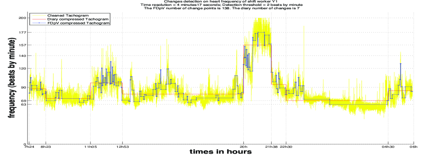
Figure 5.10: Segmentation of heartbeat time series of shift worker Y1. Yellow: cleaned heart rate. Blue: heart rate segmented by FDpV. Red: Heart rate segmented following the dairy.

Fig. 5.10 is concerned with heart beats of a shift worker Y1 through out a day its the life. The shift worker Y1 has manually reported changes of activity on a diary, as shown in Table 5.2.

Time	7h24-8h23	8h23-11h05	11h05-12h53	12h53-20h	20h-21h38	22h30-4h30
Activity	Task 1	Task 2	Picking	Free afternoon	playing football	Sleeping

Table 5.2: A shift worker’s activities record

In yellow, we have plotted the cleaned heart rate time series. In red, we have plotted the segmentation resulting from manually recorded diary. In blue, we have plotted the automatic segmentation resulting from FDpV method. Note that the computation time is 15 seconds for 120,000 data with a code written in Matlab in a 2.8 GHz processor. Moreover, the FDpV segmentation is more accurate than the manual one. For instance, Y1 has reported "Football training" from 20h to 21h38, which is supported by our analysis. But with FDpV method, we can see more details of the training namely the warming-up, the time for coach’s recommendations, and the football game with two small breaks.

Let us remark once again that both heartbeat time series and wavelet coefficient series do not fulfill the assumption of independency. However, FDpV segmentation provides accurate information on the heart rate, letting suppose a certain robustness of the method with respect to the stochastic model.

In this case, the FD-pV method has the advantage of being a fast and automatic procedure of segmentation of a large dataset, on the mean in this example, but possibly on the slope or the variance. Combined with the "tachogram cleaning" algorithm, we then have an entirely automatic procedure to obtain apparently homogeneous segment. The next step will be to detect change on hidden structural parameters. First attempts in this direction are exposed in Ayache and Bertrand (2011) and Khalfa et al. (2011), but should be completed by forthcoming studies.

Changes in the average daily volume

Trading volume represents number of shares or contracts traded in a financial market during a specific period. Average traded volume is an important indicator in technical analysis as it is used to measure the worth of a market move. If the markets move significantly up or down, the perceived strength of that move depends on the volume of trading in that period. The higher the volume during that price move, the more significant the is move. Therefore, the detection of abrupt changes in the average daily volume provide relevant information for financial engineer, trader, etc. Then, we consider here a daily volume of Carbone Lorraine compagny observed during 02 January 2009. These data have been kindly given by Charles-Albert Lehalle from Crédit Agricole Cheuvreux, Groupe CALYON (Paris). The results obtained with our algorithm for $A=300$, $p_{1}^{*}=0.05$ and $p_{2}^{*}=10^{-5}$ are illustrated in Figure 5.11. It appears that FDp-V procedure detects major changes observed after each huge variations. In future works, we will investigate sequential detection of change points in the average daily volume in connection with the worth of a market move.

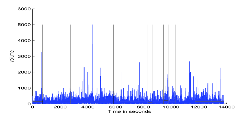
Figure 5.11: Segmentation of the daily volume of Carbone Lorraine compagny observed during 02 January 2009.

Remark 5.1

We note that in our procedure, the observations are assumed to be independent. However, by Durbin and Watson test, we show that this condition is not checked, and we obtain a global correlation $\rho_{\text{Heartbeat}}=0.9982$ for the heartbeat data, and $\rho_{\text{volume}}=0.4663$ for the financial time series. But this is not a restriction, on the contrary, this shows the robustness of our algorithm. In future works, this algorithm may be adapted to dependent data.

CONCLUSION

It appears that both methods, namely FDp-V and PLSC, give right results with practically the same precision. But, when we compare the complexity, we remark that the FDp-V method is less expensive in terms of time and memory complexity. Consequently, FDp-V method is faster (time) and cheaper (memory), and so it is more adapted to segment random signals with large or huge datasets.

In future works, we will develop the Filtered Derivative with p-value method in order to detect abrupt changes in parameters of weakly or strongly dependent time series. In particularly, we will consider the detection problem on the Hurst parameter of multifractional Brownian motion and apply it to physiological data as in Billat et al. (2009). Let us also mention that the FDp-V method is based on sliding window and could be adapted to sequential detection, see for instance Bertrand and Fleury (2008); Bertrand and Fhima (2009).

6 PROOF

Proof of Theorem 3.1. Under the null hypothesis $(H_{0})$ the filtered derivative can be rewritten as follows

$$\frac{\sqrt{A_{n}}}{\sigma}D_{1}(k,A_{n})=\frac{S_{k-A_{n}}-2S_{k}+S_{k+A_{n}}}{\sqrt{A_{n}}},$$

where $\displaystyle S_{k}=\sum_{j=1}^{k}\xi_{j}$, with $(\xi_{j})_{j\in[1,n]}$ a sequence of i.i.d r.v such as $\mathbb{E}[\xi_{1}]=0$, $\mathbb{E}[\xi_{1}^{2}]=1$, $S_{0}=0$.

To achieve our goal, we state three lemmas. First, we show in Lemma 6.1 that if a positive sequence $(a_{n})$ has the following asymptotic distribution

$$\lim\limits_{\begin{subarray}{c}n\to+\infty\end{subarray}}\mathbb{P}\left(a_{n}\leq c_{n}(x)\right)=\exp(-2e^{-x}),$$

where $c_{n}(.)$ is defined by $\eqref{cnx}$ and if there is a second positive sequence $(b_{n})$ which converges almost surely (a.s) to $(a_{n})$ with rate of convergence of order $\mathcal{O}\left(\sqrt{\log n}\right)$, then $(b_{n})$ has the same asymptotic distribution as $(a_{n})$. We then prove in Lemma 6.2 that under one of the assumptions $(\mathcal{A}_{i})$ with $i\in\{1,2,3\}$, the maximum of the increment $\displaystyle\frac{\sqrt{A_{n}}}{\sigma}\left|D_{1}(k,A_{n})\right|$ converges a.s. to the maximum of discrete Wiener process’ increment with rate $\mathcal{O}\left(\sqrt{\log n}\right)$. We show in Lemma 6.3 that the maximum of discrete Wiener process’ increment converges a.s. to the maximum of continuous Wiener process’ increment with rate $\mathcal{O}\left(\sqrt{\log n}\right)$. Then, by applying Qualls and Watanabe (1972, Theorem 5.2, p. 594), we deduce the asymptotic distribution of the maximum of continuous Wiener process’ increment. Finally, by combining these results, we get directly $\eqref{lim:mu}$.
To begin with, let us state the first lemma.

Lemma 6.1

Let $(a_{n})$ and $(b_{n})$ two sequences of positive random variables and we denote $\eta_{n}=|a_{n}-b_{n}|$.
We assume that

1. $\lim\limits_{\begin{subarray}{c}n\to+\infty\end{subarray}}\mathbb{P}\left(a_{n}\leq c_{n}(x)\right)=\exp(-2e^{-x}).$

2. $\lim\limits_{\begin{subarray}{c}n\to+\infty\end{subarray}}\eta_{n}\sqrt{\log n}\stackrel{{\scriptstyle a.s}}{{=}}0.$

where $c_{n}(.)$ is defined by $\eqref{cnx}$. Then

$$\lim\limits_{\begin{subarray}{c}n\to+\infty\end{subarray}}\mathbb{P}\left(b_{n}\leq c_{n}(x)\right)=\exp(-2e^{-x}).$$ (6.1)

$\lozenge$

Proof of Lemma 6.1. Without any restriction, we can consider the case where $\eta_{n}>0$. We denote by $|\Delta x|$ an infinitesimally small change in $x$. Then, for $n$ large enough and $|\Delta x|$ small enough, $c_{n}\left(x+|\Delta x|\right)$ and $c_{n}\left(x-|\Delta x|\right)$ satisfy the following inequalities

$$c_{n}\left(x+|\Delta x_{n}|\right) \geq c_{n}(x)+\frac{|\Delta x_{n}|}{\sqrt{2\log n}},$$ (6.2)

$$c_{n}\left(x-|\Delta x_{n}|\right) \leq c_{n}(x)-\frac{|\Delta x_{n}|}{\sqrt{2\log n}}.$$ (6.3)

Following Chen (1988), we supply a lower and an upper bounds of $\displaystyle\mathbb{P}\left(b_{n}\leq c_{n}(x)\right)$. On the one hand, by using the inequality $\eqref{ineg1}$, the upper bound results from the following calculations

$$\displaystyle\mathbb{P}\left(b_{n}\leq c_{n}(x)\right) \leq \displaystyle\mathbb{P}\left(b_{n}\leq c_{n}\left(x+|\Delta x|\right)-\frac{|\Delta x|}{\sqrt{2\log n}}\right)$$

$$\leq \displaystyle\mathbb{P}\left(a_{n}-\eta_{n}\leq c_{n}\left(x+|\Delta x|\right)-\frac{|\Delta x|}{\sqrt{2\log n}}\right)$$

$$\leq \displaystyle\mathbb{P}\left(a_{n}\leq c_{n}\left(x+|\Delta x|\right)\right)+\mathbb{P}\left(-\eta_{n}\leq-\frac{|\Delta x|}{\sqrt{2\log n}}\right)$$

$$= \displaystyle\mathbb{P}\left(a_{n}\leq c_{n}\left(x+|\Delta x|\right)\right)+\mathbb{P}\left(\eta_{n}\geq\frac{|\Delta x|}{\sqrt{2\log n}}\right).$$

On the other hand, by using the inequality $\eqref{ineg2}$, the lower bound results from analogous calculations

$$\displaystyle\mathbb{P}\left(a_{n}\leq c_{n}\left(x-|\Delta x_{n}|\right)\right) \leq \displaystyle\mathbb{P}\left(b_{n}\leq c_{n}(x)\right)+\mathbb{P}\left(\eta_{n}\geq\frac{|\Delta x_{n}|}{\sqrt{2\log n}}\right).$$

Then, by putting together the two previous bounds, we obtain

$$\mathbb{P}\left(a_{n}\leq c_{n}\left(x-|\Delta x_{n}|\right)\right)-\mathbb{P}\left(\eta_{n}\geq\frac{|\Delta x_{n}|}{\sqrt{2\log n}}\right) \leq \mathbb{P}\left(b_{n}\leq c_{n}(x)\right)$$

$$\leq \mathbb{P}\left(a_{n}\leq c_{n}\left(x+|\Delta x_{n}|\right)\right)+\mathbb{P}\left(\eta_{n}\geq\frac{|\Delta x_{n}|}{\sqrt{2\log n}}\right).$$

Finally, by taking the limit in $n$ and as $|\Delta x|$ is arbitrary small, we deduce $\eqref{lim:lem1}$. This finishes the proof of Lemma 6.1. $\blacklozenge$

Now, we show that the maximum of $\frac{\sqrt{A_{n}}}{\sigma}\left|D_{1}(k,A_{n})\right|$ converges a.s to the maximum of discrete Wiener process’ increment with rate of convergence of order $\mathcal{O}\left(\sqrt{\log n}\right)$. This is stated in Lemma 6.2 below (which gives also corrections to previous results of Chen (1988):

Lemma 6.2

Let $(W_{t},\ t\geq 0)$ be a standard Wiener process and $\displaystyle\left(Z_{A_{n}}(q),0\leq q\leq\frac{n}{A_{n}}-1\right)$ be the discrete sequence defined by

$$Z_{A_{n}}(q)=\left\{\begin{array}[]{ll}\displaystyle W_{q-1}-2W_{q}+W_{q+1}&\mbox{if }1\leq q\leq\frac{n}{A_{n}}-1,\\ 0&\mbox{else }.\end{array}\right.$$ (6.4)

Let $\displaystyle(X_{i})_{i=1,\dots,n}$ be a sequence of independent identically distributed random variables with mean $\mu$, variance $\sigma^{2}$, $D_{1}$ be defined by $\eqref{def:D1}$, and denote

$$\eta_{1,n}=\left|\max_{0\leq k\leq n-A_{n}}\frac{\sqrt{A_{n}}}{\sigma}\left|D_{1}(k,A_{n})\right|-\max_{0\leq q\leq\frac{n}{A_{n}}-1}\left|Z_{A_{n}}(q)\right|\right|.$$

Moreover, we suppose that one of the assumptions $(\mathcal{A}_{i})$, with $i\in\{1,2,3\}$ is in force. Then there exists a Wiener process $(W_{t})_{t}$ such that

$$\lim\limits_{\begin{subarray}{c}n\to+\infty\end{subarray}}\eta_{1,n}\sqrt{\log n}\stackrel{{\scriptstyle a.s}}{{=}}0.$$ (6.5)

$\lozenge$

Proof of Lemma 6.2. We consider a new discrete sequence, $\left(B(k,A_{n}),0\leq k\leq n-A_{n}\right)$, obtained by scaling from the sequence $\left(Z_{A_{n}}(q),0\leq q\leq\frac{n}{A_{n}}-1\right)$. It is defined as follows

$$B(k,A_{n})=\left\{\begin{array}[]{ll}\displaystyle\frac{W_{k-A_{n}}-2W_{k}+W_{k+A_{n}}}{\sqrt{A_{n}}}&\mbox{if }A_{n}\leq k\leq n-A_{n}\\ 0&\mbox{else }\end{array}\right.\\$$

Then

$$\eta_{1,n}\stackrel{{\scriptstyle\mathcal{D}}}{{=}}\left|\max_{0\leq k\leq n-A_{n}}\frac{\sqrt{A_{n}}}{\sigma}\left|D(k,A_{n})\right|-\max_{0\leq k\leq n-A_{n}}\left|B(k,A_{n})\right|\right|,$$

where the sign $\stackrel{{\scriptstyle\mathcal{D}}}{{=}}$ means equality in law. Depending on which assumption $(\mathcal{A}_{i})$ is in force, we have three different proofs:

1. Assuming $\mathbf{(\mathcal{A}_{1})}$.
   This is the simplest case. We can choose a standard Wiener process, $(W_{t},\ t\geq 0)$, such that $S_{k}=W_{k}$ at all the integers $k\in[0,n-A_{n}]$. Hence, $\frac{\sqrt{A_{n}}}{\sigma}D(k,A_{n})=B(k,A_{n})$. Then, we can deduce $\eqref{lim:eta1}$.

2. Assuming $\mathbf{(\mathcal{A}_{2})}$.
   We have

   $$0\leq\eta_{1,n}\leq\max_{0\leq k\leq n-A_{n}}\left|D(k,A_{n})-B(k,A_{n})\right|\leq\frac{4}{\sqrt{A_{n}}}\max_{0\leq k\leq n-A_{n}}\left|S_{k}-W_{k}\right|$$

   and after

   $$0\leq\eta_{1,n}\sqrt{\log n}\leq\frac{4(\log n)^{\frac{3}{2}}}{\sqrt{A_{n}}}\times\frac{\displaystyle\max_{0\leq k\leq n-A_{n}}\left|S_{k}-W_{k}\right|}{\log n}$$

   However, $\lim\limits_{\begin{subarray}{c}n\to+\infty\end{subarray}}\frac{(\log n)^{3}}{A_{n}}=0$ and according to Komlós et al. (1975, Theorem 3, p.34), there is a Wiener process, $(W_{t},\ t\geq 0)$, such as $\lim\limits_{\begin{subarray}{c}n\to+\infty\end{subarray}}\frac{{\displaystyle\max_{0\leq k\leq n}}\left|S_{k}-W_{k}\right|}{\log n}<+\infty.$ Then, we can deduce $\eqref{lim:eta1}$.

3. Assuming $\mathbf{(\mathcal{A}_{3})}$.
   By using the same tricks than in the proof of the case $(\mathcal{A}_{2})$, we can show that

   $$0\leq\eta_{1,n}\sqrt{\log n}\leq\frac{4n^{\frac{1}{p}}\sqrt{\log n}}{\sqrt{A}}\times\frac{\displaystyle\max_{0\leq k\leq n-A_{n}}\left|S_{k}-W_{k}\right|}{n^{\frac{1}{p}}}$$

   However, $\displaystyle\lim\limits_{\begin{subarray}{c}n\to+\infty\end{subarray}}\frac{n^{\frac{2}{p}}\log n}{A_{n}}=0$ and according to Komlós et al. (1975, Theorem 3, p.34), there is a Brownian motion, $(W_{t},\ t\geq 0)$, such as $\displaystyle\lim\limits_{\begin{subarray}{c}n\to+\infty\end{subarray}}\frac{\displaystyle\max_{0\leq k\leq n}\left|S_{k}-W_{k}\right|}{n^{\frac{1}{p}}}<+\infty.$ Then, we can deduce (6.5).

This finishes the proof of Lemma 6.2. $\blacklozenge$
In order to apply Qualls and Watanabe (1972, Theorem 5.2, p. 594) theorem, we have to consider a continuous version of the process $Z_{A_{n}}$. For this reason, we define the continuous process $\displaystyle\left(Z_{A_{n}}(t),t\in\left[0,\frac{n}{A_{n}}-1\right]\right)$ such as

$$Z_{A_{n}}(t)=W_{t-1}-2W_{t}+W_{t+1}.$$ (6.6)

Then, in Lemma 6.3, we show that the maximum of $\displaystyle\left|Z_{A_{n}}(q)\right|$ converges a.s to the maximum of $\displaystyle\left|Z_{A_{n}}(t)\right|$ with rate of convergence of order $\mathcal{O}\left(\sqrt{\log n}\right)$.

Lemma 6.3

Let $Z_{A_{n}}$ be defined by (6.4) and set $\displaystyle\eta_{2,n}=\left|\sup_{t\in\left[0,\frac{n}{A_{n}}-1\right]}\left|Z_{A_{n}}(t)\right|-\max_{0\leq q\leq\frac{n}{A_{n}}-1}\left|Z_{A_{n}}(q)\right|\right|.$
Then

$$\lim\limits_{\begin{subarray}{c}n\to+\infty\end{subarray}}\eta_{2,n}\sqrt{\log n}\stackrel{{\scriptstyle a.s}}{{=}}0.$$ (6.7)

$\lozenge$

Proof of Lemma 6.3. We have

$$0\leq\eta_{2,n}\leq 4\sup_{t\in\left[0,\frac{n}{A_{n}}-1\right]}\left|W_{t+1}-W_{t}\right|\leq 4\sup_{t\in\left[0,\frac{n}{A_{n}}-\frac{1}{A_{n}}\right]}\sup_{s\in\left[0,\frac{1}{A_{n}}\right]}\left|W_{t+s}-W_{t}\right|.$$

This implies

$$0\leq\eta_{2,n}\sqrt{\log n}\leq 4\sqrt{\log n}\sup_{t\in\left[0,\frac{n}{A_{n}}-\frac{1}{A_{n}}\right]}\sup_{s\in\left[0,\frac{1}{A_{n}}\right]}\left|W_{t+s}-W_{t}\right|$$

and after

$$\mathbb{P}\left(\eta_{2,n}\sqrt{\log n}\geq\delta\right)\leq\mathbb{P}\left(\sup_{t\in\left[0,\frac{n}{A_{n}}-\frac{1}{A_{n}}\right]}\sup_{s\in\left[0,\frac{1}{A_{n}}\right]}\left|W_{t+s}-W_{t}\right|\geq\frac{\delta\sqrt{A_{n}}}{4\sqrt{\log n}}\frac{1}{\sqrt{A_{n}}}\right)$$

According to Csörgö and Révész (1981, Lemma 1.2.1, p. 29), and by taking $\displaystyle T=n/A_{n}$, $\displaystyle h=1/A_{n}$, $\varepsilon=1$, $\displaystyle\nu=\frac{\delta\sqrt{A_{n}}}{4\sqrt{\log n}}$, and $C$ a non negative real, we deduce that

$$\mathbb{P}\left(\eta_{2,n}\sqrt{\log n}\geq\delta\right)\leq C\frac{n}{A_{n}}\exp\left(-\frac{\delta^{2}A_{n}}{48\log n}\right).$$

Next, by using $\lim\limits_{\begin{subarray}{c}n\to+\infty\end{subarray}}\frac{(\log n)^{2}}{A_{n}}=0,$ we can deduce

$$\sum_{n\geq 1}\frac{n}{A_{n}}\exp\left(-\frac{\delta^{2}A_{n}}{48\log n}\right)<+\infty,$$

and after

$$\sum_{n\geq 1}\mathbb{P}\left(\eta_{2,n}\sqrt{\log n}\geq\delta\right)<+\infty.$$

Then, according to Borel-Cantelli lemma, we can deduce $\eqref{lim:eta2}$. This finishes the proof of Lemma 6.3. $\blacklozenge$
Next, we apply Qualls and Watanabe (1972, Theorem 5.2, p. 594) to the continuous process $\displaystyle\left|Z_{A_{n}}(t)\right|.$ We obtain the asymptotic distribution of its maximum given by

$$\lim\limits_{\begin{subarray}{c}n\to+\infty\end{subarray}}\mathbb{P}\left(\sup_{t\in\left[0,\frac{n}{A}-1\right]}\left|Z_{A_{n}}(t)\right|\leq c_{n}(x)\right)=\exp(-2e^{-x}).$$ (6.8)

This result can be proved by applying Theorem 5.2 of Qualls and Watanabe (1972) to the centered stationary Gaussian process $\left(Z_{A_{n}}(t),t\geq 0\right)$. The covariance function of $Z_{A_{n}}(t)$ is given by

$$\rho(\tau)=\frac{Cov\left(Z_{A_{n}}(t),Z_{A_{n}}(t+\tau)\right)}{\sqrt{Var\left(Z_{A_{n}}(t)\right)}\sqrt{Var\left(Z_{A_{n}}(t+\tau)\right)}}=\left\{\begin{array}[]{ll}1-|\tau|&\mbox{if }0\leq|\tau|\leq 1,\\ \displaystyle-1+\frac{|\tau|}{2}&\mbox{if }1<|\tau|\leq 2,\\ 0&\mbox{if }2<|\tau|<+\infty.\\ \end{array}\right.$$

So, the conditions of Theorem 5.2 of Qualls and Watanabe (1972) are satisfied in the following way: $\alpha=1$, $H_{\alpha}=1$ (according to Pickands (1969, p. 77), and $\widetilde{\sigma}^{-1}(x)=2x^{-2}$. This finishes the proof of $\eqref{lim:Zt}$.

Eventually, by combining Lemma 6.1, Lemma 6.3 and result $\eqref{lim:Zt}$, we get the asymptotic distribution of the maximum of the sequence $\displaystyle\left(|Z_{A_{n}}(q)|,0\leq q\leq\frac{n}{A_{n}}-1\right)$. Then, by using Lemma 6.1 and Lemma 6.2, we immediately get the distribution of the maximum of the filtered derivative sequence $(|D_{1}(A_{n},k)|,0\leq k\leq n-A_{n}).$ $\blacksquare$
End of the proof of Theorem 3.1.

Proof of Theorem 3.2. Fix $\varepsilon>0$, the key argument is to divide $\Omega$ into two complementary events

$$\Omega_{1,n}=\left\{|\sigma-\widehat{\sigma}_{n}|\log n\leq\sigma\varepsilon\right\}\qquad\mathrm{and}\qquad\Omega_{2,n}=\left\{|\sigma-\widehat{\sigma}_{n}|\log n>\sigma\varepsilon\right\}.$$

Then, we have

$$\mathbb{P}\left(\max_{k\in[A_{n}:n-A_{n}]}|D_{1}(k,A_{n})|\leq\frac{\widehat{\sigma}_{n}}{\sqrt{A_{n}}}c_{n}(x)\right) = \mathbb{P}\left(\max_{k\in[A_{n}:n-A_{n}]}|D_{1}(k,A_{n})|\leq\frac{\widehat{\sigma}_{n}}{\sqrt{A_{n}}}c_{n}(x)\text{ and }\Omega_{1,n}\right)$$

$$+ \mathbb{P}\left(\max_{k\in[A_{n}:n-A_{n}]}|D_{1}(k,A_{n})|\leq\frac{\widehat{\sigma}_{n}}{\sqrt{A_{n}}}c_{n}(x)\text{ and }\Omega_{2,n}\right)$$

On the one hand, we remark that

$$\mathbb{P}\left(\max_{k\in[A_{n}:n-A_{n}]}|D_{1}(k,A_{n})|\leq\frac{\widehat{\sigma}_{n}}{\sqrt{A_{n}}}c_{n}(x)\text{ and }\Omega_{2,n}\right)\leq\mathbb{P}\left(\Omega_{2,n}\right),$$

which combined with assumption $\eqref{lim:hyp1}$ implies that

$$\lim\limits_{\begin{subarray}{c}n\to+\infty\end{subarray}}\mathbb{P}\left(\Omega_{2,n}\right)=0.$$ (6.9)

On the other hand, for all $\omega\in\Omega_{1,n}$, we have $\displaystyle\widehat{\sigma}_{n}=\sigma(1+\lambda_{n}(\omega))$ with $\displaystyle|\lambda_{n}(\omega)|\leq\frac{\varepsilon}{\log n}.$ Therefore, $\displaystyle\lim\limits_{\begin{subarray}{c}n\to+\infty\end{subarray}}\lambda_{n}\stackrel{{\scriptstyle a.s}}{{=}}0.$ Next, by setting $\displaystyle a_{n}=\frac{\sqrt{A_{n}}}{\sigma}\max_{k\in[A_{n}:n-A_{n}]}|D_{1}(k,A_{n})|$, we get

$$\mathbb{P}\left(\max_{k\in[A_{n}:n-A_{n}]}|D_{1}(k,A_{n})|\leq\frac{\widehat{\sigma}_{n}}{\sqrt{A_{n}}}c_{n}(x)\text{ and }\Omega_{1,n}\right) = \mathbb{P}\left(a_{n}\leq c_{n}(x)(1+\lambda_{n}(\omega))\right)$$

$$= \mathbb{P}\left(a_{n}-\eta_{3,n}\leq c_{n}(x)\right)$$

with $\displaystyle\eta_{3,n}=c_{n}(x)\lambda_{n}$. Therefore, after having checked that

$$\lim\limits_{\begin{subarray}{c}n\to+\infty\end{subarray}}\eta_{3,n}\sqrt{\log n}\stackrel{{\scriptstyle a.s}}{{=}}0,$$ (6.10)

we can apply Lemma 6.1 which combined with Theorem 3.1 implies that

$$\mathbb{P}\left(\max_{k\in[A_{n}:n-A_{n}]}|D_{1}(k,A_{n})|\leq\frac{\widehat{\sigma}_{n}}{\sqrt{A_{n}}}c_{n}(x)\text{ and }\Omega_{1,n}\right)=\exp(-2e^{-x})$$

Eventually, combined with $\eqref{lim:omega2}$ this implies $\eqref{lim:mu2}$. To finish the proof, it just remains to verify that $\eqref{lim:eta3}$ is satisfied. Indeed,

$$\eta_{3,n}\sqrt{\log n}\leq\varepsilon\frac{c_{n}(x)}{\sqrt{\log n}},$$

and after having replaced $c_{n}(x)$ by its expression $\eqref{cnx}$, we can easily verify that

$$\lim\limits_{\begin{subarray}{c}n\to+\infty\end{subarray}}\eta_{3,n}\sqrt{\log n}\stackrel{{\scriptstyle a.s}}{{=}}0.$$

This finishes the proof of Theorem 3.2. $\blacklozenge$

Proof of Corollary 3.2. Let $D_{2}$ and $\widehat{D}_{2}$ be defined respectively by $\eqref{def:D2}$ and $\eqref{def:D2hat}$, and set

$$\eta_{4,n}=\left|\max_{0\leq k\leq n-A_{n}}\frac{\sqrt{A_{n}}}{\nu}\left|D_{2}(k,A_{n})\right|-\max_{0\leq k\leq n-A_{n}}\frac{\sqrt{A_{n}}}{\nu}\left|\widehat{D}_{2}(k,A_{n})\right|\right|.$$

The key argument is to prove that

$$\lim\limits_{\begin{subarray}{c}n\to+\infty\end{subarray}}\eta_{4,n}\sqrt{\log n}\stackrel{{\scriptstyle a.s}}{{=}}0.$$ (6.11)

by using assumption $\eqref{condMu}$. Then, we apply Lemma 6.1 which combined with Corollary 3.1 implies $\eqref{lim:var2}$. So, to finish the proof we must verify $\eqref{lim:eta4}$.
We have

$$0\leq\eta_{4,n}\leq\frac{\sqrt{A_{n}}}{\nu}\max_{0\leq k\leq n-A_{n}}\left|D_{2}(k,A_{n})-\widehat{D}_{2}(k,A_{n})\right|$$

which implies

$$0\leq\eta_{4,n}\leq\frac{\sqrt{A_{n}}}{\nu}\max_{0\leq k\leq n-A_{n}}\left||\mu-\widehat{\mu}_{k}|^{2}-|\mu-\widehat{\mu}_{k-A_{n}}|^{2}\right|$$

and after

$$0\leq\eta_{4,n}\sqrt{\log n}\leq\frac{2}{\nu}\max_{0\leq k\leq n-A_{n}}|\mu-\widehat{\mu}_{k}|^{2}\sqrt{A_{n}\log n}.$$

Therefore, by using condition $\eqref{condMu}$, we get

$$\lim\limits_{\begin{subarray}{c}n\to+\infty\end{subarray}}\eta_{4,n}\sqrt{\log n}\stackrel{{\scriptstyle a.s}}{{=}}0.$$

This finishes the proof of Corollary 3.2. $\blacksquare$

PROOF FOR LINEAR REGRESSION

Proof of Theorem 4.1. First we note that, under the null hypothesis $(H_{0})$, the sequence $(D_{3}(k,A_{n}))_{A_{n}\leq k\leq n-A_{n}}$ satisfy

$$AD_{3}(k,A_{n})=S_{k}^{-2}\sum_{j=k+1}^{k+A_{n}}\left(X_{j}-\overline{X}_{k}\right)\varepsilon_{j}-S_{k-A_{n}}^{-2}\sum_{j=k-A_{n}+1}^{k}\left(X_{j}-\overline{X}_{k-A_{n}}\right)\varepsilon_{j}$$

where

$$\overline{X}_{k}=A_{n}^{-1}\sum_{j=k+1}^{k+A_{n}}X_{j} S_{k}^{2}=A_{n}^{-1}\sum_{j=k+1}^{k+A_{n}}\left(X_{j}-\overline{X}_{k}\right)^{2},$$ and

are respectively the empirical mean and the empirical variance of $X$ on the (sliding) box $[k+1,\,k+A_{n}]$. By using the definition $\eqref{absXi}$, we see that

$$\overline{X}_{k}=\Delta\left(k+\frac{A_{n}+1}{2}\right) \quad\mathrm{and}\quad S_{k}^{2}=\Delta^{2}\left(\frac{A_{n}^{2}-1}{12}\right).$$

Therefore, we can deduce

$$D_{3}(k,A_{n})=\frac{12}{\Delta\times A_{n}\times(A_{n}^{2}-1)}\sum_{j=k-A_{n}+1}^{k+A_{n}}\gamma(j-k,A_{n})\varepsilon_{j}$$

where

$$\gamma(i,A_{n})=\left\{\begin{array}[]{ll}i-\frac{A_{n}+1}{2}&\mbox{if }i>0,\\ -i-\frac{A_{n}-1}{2}&\mbox{if }i\leq 0.\\ \end{array}\right.$$ (6.12)

Remark that the mean and the variance of the Gaussian sequence $(D_{3}(k,A_{n}))_{A_{n}\leq k\leq n-A_{n}}$ verify

$$\mathbb{E}\left[D_{3}(k,A_{n})\right]=0 \quad\mathrm{and}\quad Var\left[D_{3}(k,A_{n})\right]=\frac{24\sigma^{2}}{\Delta^{2}\times A_{n}\times(A_{n}^{2}-1)}.$$

Moreover the variance does not depend on $k$. Then, $(D_{3}(k,A_{n}))_{A_{n}\leq k\leq n-A_{n}}$ is a centered stationary Gaussian sequence. Next, theorem 4.1 becomes an application of Csáki and Gonchigdanzan (2002, Theorem 2.1, p. 3) which gives the asymptotic distribution of the maximum of standardized stationary Gaussian sequences $(Z_{k})_{k\geq 1}$ with covariance $\displaystyle r_{n}=\mbox{cov}\left(Z_{1},Z_{n+1}\right)$ under the condition $\displaystyle r_{n}\log(n)\rightarrow 0$. Let us define the standardized version of $D_{3}$ as

$$D_{3}^{\text{Std}}(k,A)=\frac{D_{3}(k,A)}{\sqrt{\text{Var}\left[D_{3}(k,A)\right]}}\qquad\mathrm{for}\;A_{n}\leq k\leq n-A_{n},$$ (6.13)

and its covariance

$$\Gamma(k_{1},k_{2}) = \mbox{cov}\left(D_{3}^{\text{Std}}(k_{1},A),D_{3}^{\text{Std}}(k_{2},A)\right).$$

The following lemma provides the value of the covariance:

Lemma 6.4

Let $\left(D_{3}^{\text{Std}}(k,A_{n})\right)_{A_{n}\leq k\leq n-A_{n}}$ the standardized stationary Gaussian sequence defined by $\eqref{def:D3std}$. Then, its covariance matrix denoted $\left(\Gamma(k_{1},k_{2})\right)_{1\leq k_{1},k_{2}\leq n}$ is given by

$$\Gamma(k_{1},k_{2})=\frac{6}{A_{n}(A_{n}^{2}-1)}\times\left\{\begin{array}[]{ll}f_{1}\left(|k_{2}-k_{1}|,A_{n}\right)&\mbox{if }0\leq|k_{2}-k_{1}|<A_{n}\\ f_{2}\left(|k_{2}-k_{1}|,A_{n}\right)&\mbox{if }A_{n}\leq|k_{2}-k_{1}|\leq 2A_{n}-1\\ 0&\mbox{if }2A_{n}-1<|k_{2}-k_{1}|<+\infty\\ \end{array}\right.$$

where

$$f_{1}\left(p,A_{n}\right)=\displaystyle\frac{1}{6}(A_{n}-p)(A_{n}^{2}-2A_{n}p-2p^{2}-1)+\frac{1}{12}p(3A_{n}^{2}+2p^{2}-6A_{n}p+1)$$

and

$$f_{2}\left(p,A_{n}\right)=\displaystyle-\frac{1}{12}(2A_{n}-p)(A_{n}^{2}-10A_{n}p-2p^{2}-1).$$

$\lozenge$

Proof of Lemma 6.4. First we note that, by symmetry property of covariance matrix, we can restrict ourselves to the case $k_{2}-k_{1}\geq 0$. Next, let us distinguish three different expressions of the covariance according to the value of $k_{2}-k_{1}$.

• If $k_{2}-k_{1}>2A_{n}-1$, then $\Gamma(k_{1},k_{2})=0.$

• If $0\leq k_{2}-k_{1}\leq 2A_{n}-1$, then

  $$C^{-1}\Gamma(k_{1},k_{2})=\sum_{j=k_{2}-A_{n}+1}^{k_{1}+A_{n}}\gamma(j-k_{1},A_{n})\gamma(j-k_{2},A_{n})\text{ with }C=\frac{6}{A_{n}(A_{n}^{2}-1)}$$

  By replacing $j-k_{1}$ with $u$, we get

  $$C^{-1}\Gamma(k_{1},k_{2})=\sum_{u=-A_{n}+1}^{A_{n}-k_{2}+k_{1}}\gamma(u,A_{n})\gamma(u+k_{2}-k_{1},A_{n}).$$

  But, in order to use formula $\eqref{gamma}$ we must find the case where the sign of $u$ and $u+k_{2}-k_{1}$ remain constant where $u\in[-A+1,A-k_{2}+k_{1}]$. That is why we must distinguish the following subcases

  • If $0\leq k_{2}-k_{1}\leq A_{n}-1$, then

    $$C^{-1}\Gamma(k_{1},k_{2}) = \sum_{u=-A_{n}+1}^{k_{1}-k_{2}}\gamma(\underbrace{u}_{\leq 0},A_{n})\gamma(\underbrace{u+k_{2}-k_{1}}_{\leq 0},A_{n})$$

    $$+ \sum_{u=k_{1}-k_{2}+1}^{0}\gamma(\underbrace{u}_{\leq 0},A_{n})\gamma(\underbrace{u+k_{2}-k_{1}}_{>0},A_{n})$$

    $$+ \sum_{u=1}^{A_{n}-k_{2}+k_{1}}\gamma(\underbrace{u}_{>0},A_{n})\gamma(\underbrace{u+k_{2}-k_{1}}_{>0},A_{n})$$

    and then $C^{-1}\Gamma_{k_{1},k_{2}}=f_{1}\left(k_{2}-k_{1},A_{n}\right).$

  • If $A_{n}\leq k_{2}-k_{1}\leq 2A_{n}-1$, then

    $$C^{-1}\Gamma(k_{1},k_{2})=\sum_{u=-A_{n}+1}^{A_{n}-k_{2}+k_{1}}\gamma(\underbrace{u}_{\leq 0},A_{n})\gamma(\underbrace{u+k_{2}-k_{1}}_{>0},A_{n})$$

    which implies $C^{-1}\Gamma(k_{1},k_{2})=f_{2}\left(k_{2}-k_{1},A_{n}\right).$

This finishes the proof of Lemma 6.4. $\blacklozenge$

Hence, by applying Csáki and Gonchigdanzan (2002, Theorem 2.1, p. 3) to the sequence $\left(D_{3}^{\text{Std}}(k,A_{n})\right)_{A_{n}\leq k\leq n-A_{n}}$, we can deduce that

$$\lim\limits_{\begin{subarray}{c}n\to+\infty\end{subarray}}\mathbb{P}\left(\max_{k\in[A_{n}:n-A_{n}]}|D_{3}^{\text{Std}}(k,A_{n})|\leq d_{n}(x)\right)=\exp(-2e^{-x}).$$ (6.14)

Then, by using $\eqref{def:D3std}$, we obtain $\eqref{lim:a}$. This finishes the proof of Theorem 4.1. $\blacksquare$

Proof of Corollary 4.1. First we note that, under the null hypothesis $(H_{0})$, the Filtered Derivative applied to the intercept satisfy

$$D_{4}(k,A_{n})=A_{n}^{-1}\sum_{j=k+1}^{k+A_{n}}e_{j}-A_{n}^{-1}\sum_{j=k-A_{n}+1}^{k}e_{j}.$$

Therefore, $\left(D_{4}(k,A_{n})\right)_{A_{n}\leq k\leq n-A_{n}}$ corresponds to a sequence of Filtered Derivative of the mean, applied to the particular case of i.i.d centered Gaussian r.v with known variance $\sigma^{2}$. Then, by applying Theorem 3.1 under assumption $\mathcal{A}_{1}$, we obtain $\eqref{lim:b}$. This finishes the proof of Corollary 4.1. $\blacksquare$

Proof of Corollary 4.2. Let $D_{4}$ and $\widehat{D}_{4}$ be defined respectively by $\eqref{def:D4}$ and $\eqref{def:D4hat}$, and set

$$\eta_{5,n}=\left|\max_{0\leq k\leq n-A_{n}}\frac{\sqrt{A_{n}}}{\sigma}\left|D_{4}(k,A_{n})\right|-\max_{0\leq k\leq n-A_{n}}\frac{\sqrt{A_{n}}}{\sigma}\left|\widehat{D}_{4}(k,A_{n})\right|\right|.$$

The key argument is to prove that

$$\lim\limits_{\begin{subarray}{c}n\to+\infty\end{subarray}}\eta_{5,n}\sqrt{\log n}\stackrel{{\scriptstyle a.s}}{{=}}0.$$ (6.15)

By using assumption $\eqref{condA}$. Then, we apply Lemma 6.1 which combined with Corollary 4.1 implies $\eqref{lim:b2}$. So, to finish the proof we must verify $\eqref{lim:eta5}$. Next, we have

$$0\leq\eta_{5,n}\leq\frac{\sqrt{A_{n}}}{\sigma}\max_{0\leq k\leq n-A_{n}}\left|D_{4}(k,A_{n})-\widehat{D}_{4}(k,A_{n})\right|$$

which implies

$$0\leq\eta_{5,n}\leq\frac{1}{\sqrt{A_{n}}\sigma}|a-\widehat{a}_{n}|\max_{0\leq k\leq n-A_{n}}\left|\displaystyle\sum_{j=k+1}^{k+A_{n}}X_{j}-\sum_{j=k-A_{n}+1}^{k}X_{j}\right|.$$

Then, by using $\eqref{absXi}$, we show that

$$0\leq\eta_{5,n}\leq\frac{\Delta_{n}}{\sqrt{A_{n}}\sigma}|a-\widehat{a}_{n}|\max_{0\leq k\leq n-A_{n}}\underbrace{\sum_{j=k-A_{n}+1}^{k+A_{n}}j}_{=A_{n}^{2}}$$

and after

$$\eta_{5,n}\sqrt{\log n}\leq|a-\hat{a}_{n}|A_{n}^{\frac{3}{2}}\Delta_{n}\sqrt{\log n}.$$

Therefore, by using condition $\eqref{condA}$, we get

$$\lim\limits_{\begin{subarray}{c}n\to+\infty\end{subarray}}\eta_{5,n}\sqrt{\log n}\stackrel{{\scriptstyle a.s}}{{=}}0.$$

This finishes the proof of Corollary 4.2 $\blacksquare$

Acknowledgments. We are grateful to the editors and the referees for their helpful comments. A first version of this work was presented during the "International Workshop in Sequential Methodologies" at UTT (Troyes, France, June 15-17, 2009). We would like to thank both organizers and participants of this conference for stimulating discussions and suggestions.

REFERENCES

- Antoch and Hušková (1994) Antoch, J. and Hušková, M. (1994). Procedures for the detection of multiple changes in series of independent observations. In Asymptotic statistics (Prague, 1993), Contrib. Statist., pages 3–20. Physica, Heidelberg.
- Ayache and Bertrand (2011) Ayache, A. and Bertrand, P. R. (2011). Discretization error of wavelet coefficient for fractal like process. Advances in Pure and Applied Mathematics, to appear.
- Bai and Perron (1998) Bai, J. and Perron, P. (1998). Estimating and testing linear models with multiple structural changes. Econometrica, 66(1):47–78.
- Basseville and Nikiforov (1993) Basseville, M. and Nikiforov, I. V. (1993). Detection of abrupt changes: theory and application. Prentice Hall Information and System Sciences Series. Prentice Hall Inc., Englewood Cliffs, NJ.
- Ben-Yaacov and Eldar (2008) Ben-Yaacov, E. and Eldar, Y. C. (2008). A fast and flexible method for the segmentation of acgh data. Bioinformatics, 24:139–145.
- Benveniste and Basseville (1984) Benveniste, A. and Basseville, M. (1984). Detection of abrupt changes in signals and dynamical systems: some statistical aspects. In Analysis and optimization of systems, Part 1 (Nice, 1984), volume 62 of Lecture Notes in Control and Inform. Sci., pages 145–155. Springer, Berlin.
- Bertrand (2000) Bertrand, P. R. (2000). A local method for estimating change points: the “hat-function”. Statistics, 34(3):215–235.
- Bertrand and Fhima (2009) Bertrand, P. R. and Fhima, M. (2009). Filtered derivative with p-value method for multiple change-points detection. In Proceeding of the 2nd International Workshop in Sequential Methodologies.
- Bertrand and Fleury (2008) Bertrand, P. R. and Fleury, G. (2008). Detecting small shift on the mean by finite moving average. International Journal of Statistics and Management System, 3:56–73.
- Billat et al. (2009) Billat, V. L., Hamard, L., Meyer, Y., and Wesfreid, E. (2009). Detection of changes in the fractal scaling of heart rate and speed in a marathon race. Physica A, 388:3798–3808.
- Birgé and Massart (2007) Birgé, L. and Massart, P. (2007). Minimal penalties for Gaussian model selection. Probab. Theory Related Fields, 138(1-2):33–73.
- Brodsky and Darkhovsky (1993) Brodsky, B. E. and Darkhovsky, B. S. (1993). Nonparametric methods in change-point problems, volume 243 of Mathematics and its Applications. Kluwer Academic Publishers Group, Dordrecht.
- Chen (1988) Chen, X. (1988). Inference in a simple change-point model. Scienta Sinica, A31:654–667.
- Chopin (2007) Chopin, N. (2007). Dynamic detection of change points in long time series. Annals of the Institute of Statistical Mathematics, 59:349–366.
- Csáki and Gonchigdanzan (2002) Csáki, E. and Gonchigdanzan, K. (2002). Almost sure limit theorems for the maximum of stationary gaussian sequences. Stat. Prob. Letters, 58:195–203.
- Csörgo and Horváth (1997) Csörgo, M. and Horváth, L. (1997). Limit Theorem in Change-Point Analysis. J. Wiley, New York.
- Csörgö and Révész (1981) Csörgö, M. and Révész, P. (1981). Strong Approximations in Probability and Statistics. Akadémiai Kiadö, Budapest.
- Fearnhead and Liu (2007) Fearnhead, P. and Liu, Z. (2007). On-line inference for multiple change points problems. Journal of the Royal Statistical Society, 69:589–605.
- Fliess et al. (2010) Fliess, M., Join, C., and Mboup, M. (2010). Algebraic change-point detection. Applicable Algebra in Engineering, Communication and Computing, 21:131–143.
- Gombay and Serban (2009) Gombay, E. and Serban, D. (2009). Monitoring parameter change in ar(p) time series models. Journal of Multivariate Analysis, 100:715–725.
- Guédon (2007) Guédon, Y. (2007). Exploring the state sequence space for hidden markov and semi markov chains. Computational Statistics and Data Analysis, 51:2379–2409.
- Hušková and Meintanis (2006) Hušková, M. and Meintanis, S. G. (2006). Change point analysis based on the empirical characteristic functions of ranks. Sequential Analysis, 25:421–436.
- Khalfa et al. (2011) Khalfa, N., Bertrand, P. R., Boudet, G., Chamoux, A., and Billat, V. (2011). Heart rate regulation processed through wavelet analysis and change detection. some case studies. Submitted.
- Kirch (2008) Kirch, C. (2008). Bootstrapping sequential change-point tests. Sequential Analysis, 27:330–349.
- Komlós et al. (1975) Komlós, J., Major, P., and Tusnády, G. (1975). An approximation of partial sums of independent ’s and the sample . I. Z. Wahrscheinlichkeitstheorie und Verw. Gebiete, 32:111–131.
- Lavielle and Moulines (2000) Lavielle, M. and Moulines, E. (2000). Least-squares estimation of an unknown number of shifts in a time series. J. Time Ser. Anal., 21(1):33–59.
- Lavielle and Teyssière (2006) Lavielle, M. and Teyssière, G. (2006). Detection of multiple change points in multivariate time series. Lithuanian Math. J., 46:287–306.
- Lebarbier (2005) Lebarbier, E. (2005). Detecting multiple change-points in the mean of gaussian process by model selection. Signal Processing, 85:717–736.
- Montgomery (1997) Montgomery, D. (1997). Introduction to Statistical Quality Control, 3rd Edition. John Wiley & Sons, New York.
- Pickands (1969) Pickands, J. (1969). Asymptotic properties of the maximum in a stationary gaussian process. Trans. Amer. Math. Soc, 145:75–86.
- Qualls and Watanabe (1972) Qualls, C. and Watanabe, H. (1972). Asymptotic properties of gaussian processes. Ann. Math. Statist, 43:580–596.
- Révész (1990) Révész, P. (1990). Random Walks in Random and non-random enviroments. World Scientific Publishing Company.
- Steinebach and Eastwood (1995) Steinebach, J. and Eastwood, R. (1995). On extreme value asymptotics for increments of renewal processes. Journal of Statistical Planning and Inference, 45:301–312.
- Task force of the European Soc. Cardiology and the North American Society of Pacing and Electrophysiology (1996) Task force of the European Soc. Cardiology and the North American Society of Pacing and Electrophysiology (1996). Heart rate variability. Standards of measurement, physiological interpretation, and clinical use. Circulation, 93:1043–1065.