Asymptotic analysis of chaotic particle sedimentation

and trapping in the vicinity of a vertical upward streamline.

Jean-Régis Angilella

Nancy-Universités, LEMTA, CNRS UMR 7563

2 avenue de la Forêt de Haye, 54504 Vandœuvre-les-Nancy, France.

Abstract

The sedimentation of a heavy Stokes particle in a laminar plane or axisymmetric flow is investigated by means of asymptotic methods. We focus on the occurrence of Stommel’s retention zones, and on the splitting of their separatrices. The goal of this paper is to analyze under which conditions these retention zones can form, and under which conditions they can break and induce chaotic particle settling. The terminal velocity of the particle in still fluid is of the order of the typical velocity of the flow, and the particle response time is much smaller than the typical flow time-scale. It is observed that if the flow is steady and has an upward streamline where the vertical velocity has a strict local maximum, then inertialess particle trajectories can take locally the form of elliptic Stommel cells, provided the particle terminal velocity is close enough to the local peak flow velocity. These structures only depend on the local flow topology and do not require the flow to have closed streamlines or stagnation points. If, in addition, the flow is submitted to a weak time-periodic perturbation, classical expansions enable one to write the particle dynamics as a hamiltonian system with one degree of freedom, plus a perturbation containing both the dissipative terms of the particle motion equation and the flow unsteadiness. Melnikov’s method therefore provides accurate criteria to predict the splitting of the separatrices of the elliptic cell mentioned above, leading to chaotic particle trapping and chaotic settling. The effect of particle inertia and flow unsteadiness on the occurrence of simple zeros in Melnikov’s function is discussed. Particle motion in a plane cellular flow and in a vertical pipe is then investigated to illustrate these results.

Key-words : Two-phase flows, Stokes particles, sedimentation, chaotic motion, Melnikov’s method.

1 Introduction

The motion of tiny heavy particles in either laminar or turbulent flows is of major importance for the understanding of many industrial or natural flows. Even when particles do not significantly modify the surrounding flow, this topic shows many unsolved questions. When the flow is turbulent, modeling the dispersion and sedimentation of heavy particles is a difficult task which has retained much attention since the pioneering works by Csanady [1], Snyder & Lumley [2] or Maxey [3], to name but a few. In laminar flows, particle motion is also investigated for at least two reasons. First, a better understanding of particle dispersion and sedimentation in fully developped turbulence can be achieved if one understands the detailed interactions between particles and elementary flow structures like vortices or shear layers. Secondly, even in laminar flows, the behaviour of small heavy particles can be rather unexpected, and chaotic settling or permanent suspension (“trapping”) can occur. In the limit of vanishing particle Reynolds number, these complex trajectories are not due to wake effects such as vortex shedding, since the disturbance flow set up by the inclusion obeys the linear Stokes equation. They are due to the gradients of the unperturbed fluid flow, which introduce severe non-linearities into the particle motion equations.

Experiments and calculations conducted since 1900 revealed that passive heavy Stokes particles dropped in a cellular flow can be trapped in the vicinity of vertical upward streamlines and remain suspended for a long time, under the combined effect of gravity and of the hydrodynamic force (Bénard [4], Stommel [5], Simon & Pomeau [6], Cerisier et al. [7], Tuval et al. [8]). Such nearly closed trajectories are often called “Stommel retention zones”, even though they are rather loosely defined. They are the central point of the present work. Stommel investigated these structures to understand plankton settling in a lake, where wind-induced cellular motion is likely to induce strong inhomogeneities in plankton concentration. In the last decades, various numerical analyses revealed that aerosol sedimentation can display complex features, whether chaotic or not, in elementary laminar flows such as plane cellular flow (Maxey & Corrsin [9], Fung [10], Rubin et al. [11]), or ABC flow (Mac Laughlin [12]). Some of these analyses revealed that the occurrence of Stommel cells in various parts of the flow played a key role in complex particle motions. For example, some particles released in a plane cellular flow, submitted to a weak time-periodic perturbation, were observed to wander around some kind of Stommel cells, and could also be trapped temporarily within these cells, in a rather chaotic manner [10]. The occurrence of Stommel cells, as well as their role in chaotic sedimentation, is therefore a topic of interest to understand and quantify complex particle motion in simple flows.

The goal of the present paper is to derive analytical criteria giving the particle parameters for which chaotic sedimentation and/or trapping occurs, for heavy isolated Stokes particles dropped in the vicinity of a vertical streamline where Stommel retention zones are likely to form. Two-dimensional and axisymmetric divergence-free flows will be considered. The paper is organized as follows. First, particle dynamics in the vicinity of an upward streamline of any steady 2D flow is investigated (section 2). Conditions leading to the formation of retention zones are derived. Then the splitting of the separatrices of these retention zones is analyzed by means of Melnikov’s method (section 3). This analysis is applied to chaotic sedimentation in a plane cellular flow in section 4. Finally, these results are generalized to axisymmetric flows ( section 5). In the next few paragraphs we present the basic equations of particle dynamics used in this paper.

If $\vec{X}_{p}(t)$ is the particle position at time $t$, the simplest motion equation for heavy isolated Stokes particles in a fluid of infinite extent is

$$m_{p}{\vec{\ddot{X}}_{p}}=m_{p}\vec{g}+6\pi\mu_{f}\,{\mbox{a}}\Big{(}\vec{V}_{f}(\vec{X}_{p},t)-\vec{\dot{X}}_{p}\Big{)},$$

where $m_{p}$ and a denote the particle mass and radius respectively, $\mu_{f}$ is the fluid dynamical viscosity, and $\vec{V}_{f}$ is the fluid velocity field in the absence of particle. This equation is valid provided the particle Reynolds, Stokes and Taylor numbers are much smaller than unity :

$$\mbox{Re}=\frac{\mbox{a}|\vec{\dot{X}}_{p}-\vec{V}_{f}|}{\nu}\ll 1,\quad\mbox{and}\quad\mbox{St}=\frac{\mbox{a}^{2}\omega_{1}}{\nu}\ll 1,$$

$$\mbox{and}\quad\mbox{Ta}=\frac{\mbox{a}^{2}|\nabla\vec{V}_{f}|}{\nu}\ll 1,$$

so that the disturbance flow due to the inclusion is a creeping quasi-steady flow ($\omega_{1}$ is the typical time-scale of this flow). In addition, the particle density $\rho_{p}$ must be much larger than the fluid density $\rho_{f}$, so that buoyancy and pressure gradient force of the undisturbed flow can be neglected. Also, brownian motion is assumed to be negligible. The velocity field $\vec{V}_{f}$ is taken to be a steady flow submitted to a weak unsteady perturbation :

$$\vec{V}_{f}(\vec{x},t)=\vec{V}_{f}^{0}(\vec{x})+\varepsilon\,\vec{V}_{f}^{1}(\vec{x},t),\quad\quad\varepsilon\ll 1.$$

Following Fung [10] we will consider the case where $\vec{V}_{f}^{1}$ is $T$-periodic with $T=2\pi/\omega$. If $V_{0}$ denotes a typical fluid velocity and $L_{0}$ is the length scale of velocity gradients in the absence of inclusion the particle motion equation, non-dimensionalized by ($V_{0}$,$L_{0}$), is :

$$\tau\,{\vec{\ddot{X}}_{p}}=\vec{V}_{T}+\vec{V}_{f}^{0}(\vec{X}_{p})+\varepsilon\,\vec{V}_{f}^{1}(\vec{X}_{p},t)-\vec{\dot{X}}_{p}$$ (1)

without renaming $t$, $\vec{X}_{p}$ and $\vec{V}_{f}$. The parameter $\tau$ is the non-dimensional response time, which is assumed to be much smaller than unity :

$$\tau=\frac{2\rho_{p}}{9\rho_{f}}\,\frac{\mbox{a}^{2}}{\nu}\frac{V_{0}}{L_{0}}\quad{\ll 1}$$

and $\vec{V}_{T}$ is the non-dimensional terminal velocity in a fluid at rest ( $\displaystyle{\vec{V}_{T}=\frac{2\rho_{p}}{9\rho_{f}}\,\frac{\mbox{a}^{2}\vec{g}}{\nu}\,\frac{1}{V_{0}}}$), which is assumed to satisfy :

$$V_{T}=|\vec{V}_{T}|=O(1).$$

The Froude number $\tau/V_{T}=V_{0}^{2}/gL_{0}$ is therefore much smaller than unity. Also, the terminal particle Reynolds number is of order $(\mbox{a}/L_{0})\,V_{0}L_{0}/\nu$, and is therefore very small provided the flow Reynolds number $V_{0}L_{0}/\nu$ is not too large. The particle motion equation contains two independent small parameters, namely $\varepsilon$ and $\tau$. In the following we set $\tau=k\,\varepsilon$, where $k$ denotes any parameter held fixed as $\varepsilon\to 0$. Then classical asymptotic expansions [3] of the form $\vec{\dot{X}}_{p}=\vec{V}_{T}+\vec{V}_{f}^{0}+\varepsilon\vec{V}_{p}^{1}+O(\varepsilon^{2})$ lead to :

$$\vec{\dot{X}}_{p}=\vec{V}_{T}+\vec{V}_{f}^{0}(\vec{X}_{p})$$

$$+{\varepsilon\Big{(}\vec{V}_{f}^{1}(\vec{X}_{p},t)-k\,\overline{\overline{\nabla}}\vec{V}_{f}^{0}.(\vec{V}_{f}^{0}+\vec{V}_{T})\Big{)}}+O(\varepsilon^{2}).$$ (2)

The case $k=0$ corresponds to heavy particles without inertia [9][3][6] : their velocity is equal to the fluid local velocity plus $\vec{V}_{T}$. In this case the particle dynamics is non-dissipative since $div\,\vec{V}_{f}=0$. In the following we will consider the general case $k\geq 0$.

2 Formation of retention zones in plane flow

As noticed by many authors [5][9][6][10], when the flow is two-dimensional the dynamical system (2) is, to leading order, hamiltonian :

$$\vec{\dot{X}}_{p}=\left(\begin{array}[]{r}\dot{x}\\ \dot{y}\end{array}\right)=\vec{V}_{T}+\vec{V}_{f}^{0}(\vec{X}_{p})=\left(\begin{array}[]{r}\frac{\partial H}{\partial y}\\ -\frac{\partial H}{\partial x}\end{array}\right)\quad$$ (3)

where $H(x,y)=\psi^{0}(x,y)+x\,V_{T}$, and $\psi^{0}$ is the streamfunction associated to $\vec{V}_{f}^{0}$, and $x$ is the horizontal coordinate and $y$ is the upward vertical coordinate. This enables to notice the following property. Suppose $\psi^{0}(x,y)$ is of class ${\cal C}^{\infty}$ and has a vertical upward streamline ${\cal S}\,\,$(Fig. 1(a)) and a point C $\in$ ${\cal S}\,\,$where the vertical velocity $v=-\partial{\psi^{0}}/\partial x$ satisfies :

$$\frac{\partial v}{\partial x}\mbox{\small(C)} = \frac{\partial v}{\partial y}\mbox{\small(C)}=0$$ (4)

$$\frac{\partial^{2}v}{\partial x^{2}}\mbox{\small(C)}\frac{\partial^{2}v}{\partial y^{2}}\mbox{\small(C)} - \Big{(}\frac{\partial^{2}v}{\partial x\partial y}\mbox{\small(C)}\Big{)}^{2}>0$$ (5)

$$\frac{\partial^{2}v}{\partial x^{2}}\mbox{\small(C)} < 0.$$ (6)

These are the classical conditions for $v(x,y)$ to have a strict local maximum at C. We will denote $x_{c}$ and $y_{c}$ the coordinates of $C$, and $\vec{x}_{c}=(x_{c},y_{c})$ its position vector. Also, we write $V_{c}=v(C)$ (the local peak flow velocity) and assume $V_{c}>0$. Then for $V_{T}<V_{c}$ and $V_{T}$ sufficiently close to $V_{c}$, the particle trajectory at order $\varepsilon^{0}$ (Eq. (3)) takes the form of an elliptic dipole of centre C (Fig. 1(b)). If in addition vorticity is zero along ${\cal S}\,\,$, the axes of the ellipse are $(C,x)$ and $(C,y)$ and the semi-axes are

$$a=\sqrt{\frac{6(V_{c}-V_{T})}{\psi^{0}_{,xxx}\mbox{\small(C)}}}\quad\quad\mbox{and}\quad\quad b=\sqrt{\frac{2(V_{c}-V_{T})}{\psi^{0}_{,xyy}\mbox{\small(C)}}}$$ (7)

(where the coma indicates spatial differentiation).

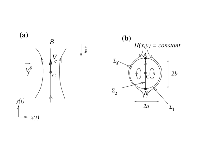
Figure 1: Sketch of the local streamlines (a) of the unperturbed flow $\vec{V}_{f}^{0}$, and of the leading order phase portrait of particle dynamics (b) in this flow, under the hypotheses listed in the text.

This property can be shown by expanding $H(x,y)$ in the vicinity of C and making use of the fact that many derivatives of $\psi^{0}$ vanish at C. First, $u(x_{c},y)=0$ for all $y\in$ ${\cal S}\,\,$, so $\partial^{n}u/\partial y^{n}(x_{c},y)=0$ for all integer $n$, so $\partial^{n}\psi^{0}/\partial y^{n}\mbox{\small(C)}$ is zero too for all $n$. Also, velocity is divergence-free, so $\psi^{0}_{,xy}\mbox{\small(C)}=u_{,x}\mbox{\small(C)}=$ $u_{,x}\mbox{\small(C)}+v_{,y}\mbox{\small(C)}=0$. Also, $\psi^{0}_{,xx}\mbox{\small(C)}=-v_{,x}\mbox{\small(C)}=0$. Therefore, by expanding $H(x,y)$ we are led to :

$$H(x,y)=\psi^{0}\mbox{\small(C)}+x_{c}\,V_{T}+(x-x_{c})$$

$$\times\Big{[}V_{T}-V_{c}+\frac{\psi^{0}_{,xxx}}{6}(x-x_{c})^{2}+\frac{\psi^{0}_{,xxy}}{2}(x-x_{c})(y-y_{c})$$

$$+\frac{\psi^{0}_{,xyy}}{2}(y-y_{c})^{2}\Big{]}+{\cal R}$$ (8)

where all the derivatives of $\psi^{0}$ have been taken at C and ${\cal R}=O(|\vec{x}-\vec{x}_{c}|^{4})$. Therefore, the isolines $H(x,y)=constant$ take locally the form of elementary curves. In particular, if ${\cal R}$ is null or negligible, the line $H(x,y)=H(C)$, for $x\not=x_{c}$, is the quadratic curve :

$$\alpha(x-x_{c})^{2}+2\beta(x-x_{c})(y-y_{c})+\gamma(y-y_{c})^{2}+\delta=0$$

where

$$\alpha=\frac{\psi^{0}_{,xxx}\mbox{\small(C)}}{6},\quad\beta=\frac{\psi^{0}_{,xxy}\mbox{\small(C)}}{4},\quad\gamma=\frac{\psi^{0}_{,xyy}\mbox{\small(C)}}{2}$$

and $\delta=V_{T}-V_{c}$. A sufficient condition for this curve to be an ellipse is : $\delta\not=0$ and $\delta(\alpha+\gamma)<0$ and $\alpha\gamma>\beta^{2}$. Assumption (6) implies $\alpha>0$, and by (5) we obtain $\gamma>0$. Also, $V_{T}<V_{c}$ means $\delta<0$. The two first ellipticity conditions are therefore fulfilled. The last one is a consequence of (5). Indeed, Eq. (5) can be re-written as $(6\alpha)(2\gamma)>(4\beta)^{2}.$ Therefore we have $\alpha\gamma>\frac{4}{3}\beta^{2},$ hence $\alpha\gamma>\beta^{2}$. If in addition vorticity is zero along ${\cal S}\,\,$, we have $\psi^{0}_{,xx}+\psi^{0}_{,yy}=0$ so $\psi^{0}_{,xx}=0$ at any point in ${\cal S}\,\,$. So $\psi^{0}_{,xxy}$ is also zero along ${\cal S}\,\,$. In particular $\beta=0$, and the ellipse has horizontal and vertical axes. In this case the semi-axes of the ellipse are $a=\sqrt{-\delta/\alpha}$ and $b=\sqrt{-\delta/\gamma}$, and this leads to (7).

The remainder ${\cal R}$ is negligible in the limit where $|\vec{x}-\vec{x}_{c}|\ll 1$. On the ellipse this condition is fulfilled if $\max(a,b)\ll 1$, that is $\mid V_{T}-V_{c}\mid\ll 1$, since both $\alpha$ and $\gamma$ are $O(1)$. Therefore, the elliptical structure is asymptotically valid if $V_{T}$ is sufficiently close to $V_{c}$. In the following we will assume that ${\cal R}$ is indeed zero or negligible, for the sake of simplicity. An analysis of the effect of ${\cal R}$ is presented in Appendix C.

Under these conditions the particle dynamics in the vicinity of C has two stagnation points $A=(x_{c},y_{c}+b)$ and $B=(x_{c},y_{c}-b)$ located along the vertical direction, related by three separatrices (heteroclinic trajectories). These cells are an example of Stommel’s retention zones, already observed with various shapes in many experimental or theoretical works cited in the introduction [4] [5] [6] [10] [7] [8]. To leading order $\varepsilon^{0}$, particles which are located within the elliptic cell are trapped and cannot exit. Also, particles released outside the cell cannot penetrate into the cell : these particles drop. Therefore, if one injects particles at random in the two-dimensional flow with a uniform distribution, the percentage of trapped particles should be approximated by the volume fraction $\Phi_{v}$ of the elliptic cells, that is :

$$\Phi_{v}=N_{e}\,\pi\,a\,b=\frac{N_{e}\,\pi\sqrt{12}}{\sqrt{\psi^{0}_{,xxx}\mbox{\small(C)}\,\psi^{0}_{,xyy}\mbox{\small(C)}}}(V_{c}-V_{T})$$ (9)

where $N_{e}$ is the number of elliptic cells per unit volume. (Since the problem is two-dimensional, volumes must be understood as surfaces multiplied by the unit length along the $z$ direction.) This formula will be checked below (section 4).

If the $O(\varepsilon)$ perturbation appearing in Eq. (2) is taken into account, the curved separatrix can be broken : particles could therefore go in and out in a quite unpredictable manner. The calculation of the parameters leading to separatrix splitting is therefore an interesting topic for the understanding of particle sedimentation, and is done in the next section.

3 Heteroclinic bifurcation and chaotic particle motion

For plane flows the particle motion equation (2) has the form of a hamiltonian system with “one-and-a-half” degree of freedom. The $O(\varepsilon^{0})$ terms contain the fluid velocity as well as the sedimentation velocity, the combined effect of which can lead to the formation of the elliptic cells described above. The separatrices of these cells form heteroclinic cycles between the stagnation points A and B. The $O(\varepsilon)$ terms manifest the effect of both the flow unsteadiness and particle inertia : clearly, these physical mechanisms might influence the particle dynamics in the vicinity of the elliptic cells, since phase portraits of the form of Fig. 1(b) can be structurally unstable.

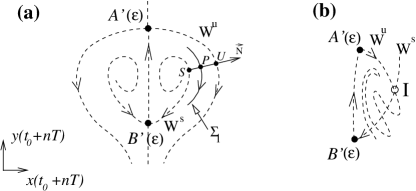
Figure 2: Sketch of the Poincaré section of the particle dynamics at order $\varepsilon$. In case (a) the manifolds do not intersect. Particles released from above the cell will not be trapped. Particles released within the cell will spiral out and exit the cell. In case (b) the manifolds intersect and chaotic sedimentation occurs.

In order to investigate analytically the role of the $O(\varepsilon)$ terms, we make use of the classical Melnikov method [13] to predict the appearance of intersection points between the stable and unstable manifolds associated to the hyperbolic points $A^{\prime}$ and $B^{\prime}$ of the Poincaré section $(x(t_{0}+nT),y(t_{0}+nT))$, $n\in\mathbf{Z}$, of the perturbed system (Fig. 2). ($T$ is the period of the perturbation velocity field : $\vec{V}_{f}^{1}(\vec{x},t+T)=\vec{V}_{f}^{1}(\vec{x})$ for all $\vec{x}$ and $t$.) Indeed, since the leading-order particle dynamics displays two hyperbolic saddle points $A$ and $B$, the Poincaré section of this system will have hyperbolic points too, at the same position $A$ and $B$. If $\varepsilon$ is small enough the Poincaré section of the perturbed system will therefore have two stagnation points of the same type (hyperbolic-saddle) $A^{\prime}(\varepsilon)$ and $B^{\prime}(\varepsilon)$, continuous functions of $\varepsilon$, by virtue of the implicit functions theorem. Accordingly, there exists stable and unstable manifolds W^s and W^u attached to $B^{\prime}(\varepsilon)$ and $A^{\prime}(\varepsilon)$ respectively. If an unstable manifold intersects a stable one (e.g. point I of Fig. 2(b)), an infinity of such intersection points will exist, since both W^s and W^u are invariant subsets of the Poincaré application. Because the $O(\varepsilon^{0})$ phase portrait displays a heteroclinic cycle, the particle dynamics in the vicinity of the broken separatrix corresponds to a horse-shoe map, by virtue of the Smale-Birkhoff theorem, characterized by chaotic trajectories and sensitivity to initial conditions. Particles are therefore likely to penetrate into the cell or exit from it, in a chaotic manner. The occurrence of intersection points can be predicted from the asymptotic calculation of the “algebraic distance” $d(t_{0})$ between W^s and W^u. It is defined as $d(t_{0})=\vec{SU}.\vec{N}$, where $\vec{N}$ is the unit vector perpendicular to $\vec{V}_{f}^{0}+\vec{V}_{T}$ at a given (arbitrary) point $P$ of the separatrix, and such that ($\vec{V}_{f}^{0}+\vec{V}_{T},\vec{N},\vec{e}_{z}$) is right-handed, and $S$ (resp. $U$) are the intersection points between the line $(P,\vec{N}$) and W^s (resp. W^u). ($\vec{e}_{z}$ is the direct unit vector in the direction perpendicular to $(x,y)$.) These points are shown, for the separatrix $\Sigma_{1}$, in Fig. 2(a). At order $\varepsilon$ this distance is proportional to the Melnikov integral [13] :

$$M(t_{0})=\int_{-\infty}^{+\infty}\Big{[}\vec{V}_{T}+\vec{V}_{f}^{0}\Big{]}_{\vec{X}_{0}(t)}\wedge\Big{[}\vec{V}_{f}^{1}\Big{(}\vec{X}_{0}(t),t+{t_{0}}\Big{)}$$

$$-k\,\overline{\overline{\nabla}}\vec{V}_{f}^{0}.\Big{(}\vec{V}_{f}^{0}+\vec{V}_{T}\Big{)}_{\vec{X}_{0}(t)}\Big{]}\,dt$$ (10)

which is integrated along the separatrix of the unperturbed system, parametrized by $\vec{X}_{0}(t)$ with $\vec{X}_{0}(-\infty)=A$ and $\vec{X}_{0}(+\infty)=B$ and $\vec{X}_{0}(0)=P$. (Here, $\vec{u}\wedge\vec{v}$ is the triple product $\vec{e}_{z}.(\vec{u}\wedge\vec{v})$.) In particular we have $\vec{\dot{X}}_{0}=\vec{V}_{f}^{0}(\vec{X}_{0})+\vec{V}_{T}$ and $\vec{\ddot{X}}_{0}=\overline{\overline{\nabla}}\vec{V}_{f}^{0}.(\vec{V}_{f}^{0}+\vec{V}_{T})$. If particle inertia is taken into account ($k\not=0$) the perturbation is dissipative, but this does not alter the validity of Eq. (10) which only requires the unperturbed system to be non-dissipative. The Melnikov integral therefore reads :

$$M(t_{0})=\int_{-\infty}^{+\infty}\vec{\dot{X}}_{0}(t)\wedge\vec{V}_{f}^{1}\Big{(}\vec{X}_{0}(t),t+{t_{0}}\Big{)}\,dt-k\,m$$ (11)

where $m=m(V_{T})$ is independent of $t_{0}$ :

$$m(V_{T})=\int_{-\infty}^{+\infty}\vec{\dot{X}}_{0}(t)\wedge\vec{\ddot{X}}_{0}(t)\,dt.$$

This term is also independent of $\vec{V}_{f}^{1}$ and corresponds to the effect of particle inertia. Because $\vec{\dot{X}}_{0}\wedge\vec{\ddot{X}}_{0}$ is proportional to the curvature of the separatrix at $\vec{X}_{0}(t)$, the constant $m$ manifests the contribution of centrifugal effects. One can easily check that $m(V_{T})<0$ (hence $-km(V_{T})>0$) for the separatrix $\Sigma_{1}$ of Fig. 1(b), and $m(V_{T})>0$ (hence $-km(V_{T})<0$) for $\Sigma_{3}$. This means that particle inertia tends to maintain $\vec{SU}$ in the direction of $\vec{N}$ on separatrix $\Sigma_{1}$ (that is $\vec{SU}$ points outward), and in the direction of $-\vec{N}$ on separatrix $\Sigma_{3}$ (that is, $\vec{SU}$ points outward also since $\vec{N}$ points inward there, as ($\vec{V}_{f}^{0}+\vec{V}_{T},\vec{N},\vec{e}_{z}$) is right-handed). In both cases this means that inertia tends to maintain W^u at the periphery of the unperturbed cell and W^s towards the interior of the cell. In particular, this enables to conclude that in the steady case ($\omega=0$) the phase portrait of the $O(\varepsilon)$ particle dynamics takes the form of Fig. 2(a). The Stommel cell is broken because of particle inertia only : particles released above the cell will never be trapped, and particles released inside the cell will always escape : these results agree with those of Rubin et al. [11], which have been obtained for aerosols in a cellular flow field.

In the following, the Melnikov integral is calculated in the case where ${\cal R}=0$ in Eq. (8), and for the elliptic separatrix $\Sigma_{1}$ of Fig. 1(b). Also, the constant $\beta$ is taken to be zero, for the sake of simplicity. The calculation of $\vec{X}_{0}(t)$ is shown in Appendix A and we are led to :

$$m(V_{T})=-2\pi\sqrt{3}\sqrt{\frac{\psi^{0}_{,xyy}\mbox{\small(C)}}{\psi^{0}_{,xxx}\mbox{\small(C)}}}\Big{(}V_{T}-V_{c}\Big{)}^{2}.$$ (12)

We observe that $m(V_{T})$ is proportional to the ratio $a/b$ (if $V_{T}-V_{c}$ is held fixed), so that flat horizontal ellipses ($b\ll a$) will be more sensitive to particle inertia than flat vertical ellipses ($b\gg a$), as expected for a centrifugal effect.

The non-constant part of the Melnikov function requires to specify the kind of perturbation applied. In this paper, “homothetic” perturbations of the form (Fung [10])

$$\vec{V}_{f}^{1}(\vec{x},t)=\vec{V}_{f}^{0}(\vec{x})\,\sin\omega t,$$ (13)

will be considered. This corresponds to flows with variable intensity without any change in the shape of the streamlines. Clearly, there is no chaotic advection of pure tracers in this flow, but it will be shown below that chaotic particle sedimentation will occur. In the case of a homothetic perturbation the term $\vec{V}_{f}^{0}\wedge\vec{V}_{f}^{1}$ vanishes, and calculations lead to $M(t_{0})=-A(\omega,V_{T}){\cos\omega t_{0}}-k\,m(V_{T})$, where $A(\omega,V_{T})$ is proportional to the Fourier transform of the horizontal component of $\vec{X}_{0}(t)$ and reads (see Appendix A) :

$$A(\omega,V_{T})=\frac{\sqrt{3}}{\sqrt{\psi^{0}_{,xyy}\,\psi^{0}_{,xxx}}}\frac{\pi\,V_{T}\,\omega}{\mbox{cosh}\frac{\pi\omega}{2\sqrt{2}\sqrt{\psi^{0}_{,xyy}(V_{c}-V_{T})}}},$$ (14)

where derivatives of $\psi^{0}$ have been taken at C. Clearly, if $A(\omega,V_{T})<k\,\mid m(V_{T})\mid$ the Melnikov integral does not have any zero, and this provides an analytical criterion to predict the splitting of the curved separatrix of the retention zone. It also enables to predict the lowest velocity $V_{T}$ below which no chaotic trapping can occur (see appendix B). Note again that these calculations are expected to be valid either if ${\cal R}\equiv 0$ or if $V_{T}$ is sufficiently close to $V_{c}$. These results will be used in section 4 and compared to numerical solutions of Eq. (1).

4 Application to plane flows

In order to validate the above results we have computed numerical particle trajectories for various plane flows, and checked whether chaotic settling appears for the parameters predicted by Melnikov’s analysis. The results are particularly accurate when the basic flow is itself a third-order polynomial function of $(x,y)$, e.g. for a cellular flow of the form $\psi^{0}(x,y)=x(x^{2}+y^{2}-1),$ since the Taylor expansion (8) is exact there. Results are also satisfactory for various non-polynomial flows, provided $\mid V_{T}-V_{c}\mid$ is small enough. Consider for example the streamfunction $\psi^{0}(x,y)=\sin x\,\sin y,$ already investigated by several authors (Maxey & Corrsin [9], Fung [10], Rubin et al. [11]). One can easily check that there is an array of upward vertical streamlines in the unperturbed velocity field, for example : $x=0$ and $-\pi\leq y\leq 0$. The vorticity is zero on this streamline and the upward velocity has a maximum at C = $(0,-\pi/2)$. Also, one can easily check that Eqs. (4)-(5)-(6) are satisfied at C = $(0,-\pi/2)$, and that $V_{c}=1$. So if $V_{T}<1$, and $V_{T}$ close to 1, the particle trajectories at order $\varepsilon^{0}$ in the vicinity of C take the form of elliptic dipolar vortices with half-axes given by Eq. (7) :

$$a=\sqrt{6(1-V_{T})}\quad\mbox{and}\quad b=\sqrt{2(1-V_{T})}.$$

Figure 3(a) shows typical numerical trajectories in this flow when $V_{T}=0.8$, in the steady case and with very small particle inertia ($\tau=0.002$). The Stommel cell is clearly visible, in agreement with the numerical computations of Refs. [5][9][10]. The ellipse of semi-axes $a$ and $b$ is also plotted for comparison.

Figure 3: Upper graph : typical particle trajectories when $V_{T}=0.8$, $\omega=0$, $\varepsilon=0.001$ and $k=2$ (thick solid lines, numerical computation). Thin solid lines are flow streamlines. The dashed line is the ellipse corresponding to the analytical result (7). Some particles have been released above the cell, others have been released inside the cell. Lower graph : trajectories of two particles released slightly above the cell when $\varepsilon=0.03$, $\tau=0.06$ and $\omega=0.5$.

In order to check the theoretical result (9), which is a direct consequence of the appearance of the elliptic cells, we have uniformly released 5000 particles within the domain $[-\pi,\pi]^{2}$ and solved numerically the full motion equation (1) in the steady case ($\omega=0$), and with a finite but small particle response time $\tau$. Then particles above the horizontal line $y=-\pi$ at time $t$ have been called “suspended”. The percentage of suspended particles for large $t$ is expected to be close to the volume fraction of the elliptic cells $\Phi_{v}$. Figure 4 shows this percentage versus $t$, together with $\Phi_{v}$ (Eq. (9) with $N_{e}=2/(2\pi)^{2}$ since there are two elliptic cells in each periodic box), for $V_{T}=0.8$, and in the cases $\tau=0.001$ and $\tau=0.05$. Clearly, the percentage of suspended particles is close to $\Phi_{v}$ for long times, but keeps on decaying because of particle inertia effects. The decay is almost undistinguishable for $\tau=0.001$ but is clearly visible for $\tau=0.05$. Indeed, since $\tau$ is finite in the numerical solution, the Poincaré section of particle dynamics is of the form of figure 2(a), since the Melnikov function $M(t_{0})=-km$ is constant and non-zero in the steady case, so that the elliptic cells are not completely closed and tend to slowly empty under the effect of particle inertia alone (see also Rubin et al. [11]).

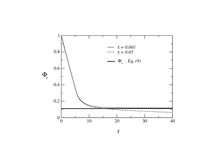
Figure 4: Decay of the percentage of suspended particles in a steady cellular flow (numerical solution of Eq. (1)), with $V_{T}=0.8$. The solid line is the analytical result (9) corresponding to $\tau=0$.

In the unsteady case ($\omega>0$) the diagram $(\omega,V_{T})$ indicating the occurrence of separatrix splitting is obtained by plotting the curve $A(\omega,V_{T})-|k\,m(V_{T})|=0$ where $A(\omega,V_{T})$ is the amplitude of the Melnikov function (14) and $k\,m$ is its constant part. This diagram is shown in Fig. 5 in the case ($k=2$). If $(\omega,V_{T})$ is located in the zone $A(\omega,V_{T})-|k\,m(V_{T})|>0$ then the separatrix is broken and particles can penetrate into the elliptic cell in an unpredictable manner : “chaotic trapping” occurs. The lowest terminal velocity below which no chaotic trapping is expected to occur is given by the analytical expression obtained in Appendix B, and is approximately $V_{T}\approx 0.76$.

Figure 5: Plot of the bifurcation diagram given by Melnikov’s analysis for sedimentation in the plane cellular flow.

In order to compare these predictions of separatrix splitting with numerical solutions we have solved Eq. (1) with an implicit Runge-Kutta algorithm, for 500 particles released at $t=0$ above the elliptic cell. For $t>0$ these particles drop and go round the elliptic cell, but some of them are likely to penetrate inside in case of separatrix splitting, and this will significantly increase the length of their path. The computation of each inclusion is stopped if the particle reaches the “ground” $y=-\pi$ or if $t=t_{f}\gg 1$ (here, $t_{f}=50$). We then measure the relative normalized averaged particle path length :

$$\theta(\omega)=\frac{{\cal L}(\omega)-{\cal L}(0)}{{\cal L}(0)},$$ (15)

where ${\cal L}(\omega)$ is the length of the particle path averaged over the particles. This quantity is good indicator of the occurrence of separatrix splitting here. Indeed, if no trapping occurs then $\theta(\omega)\simeq 0$, because all particle paths are rather similar (they look like those of figure 3(a)). If trapping occurs, some particles will spin inside the cell for a while (like in figure 3(b)) and this will increase $\theta(\omega)$.

Figure 6: Plot of the numerical computation of the averaged particle path length in the unsteady plane cellular flow $\psi^{0}=\sin x\sin y$ (black dots), together with $A(\omega,V_{T})-k|m(V_{T})|$ (solid line, analytical expressions (12) and (14)). The fluid velocity at C is $V_{c}=1$, and $\tau=0.06$, $\varepsilon=0.03$, ($k=2$).

Fig. 6 shows $\theta(\omega)$ versus $\omega$ (black dots), together with $A(\omega,V_{T})-|k\,m(V_{T})|$ (solid line), the positive values of which imply separatrix splitting (here $\varepsilon=0.03$ and $\tau=0.06$). Clearly, when $A(\omega,V_{T})-|k\,m(V_{T})|>0$ some particles are trapped, and when $A(\omega,V_{T})-|k\,m(V_{T})|<0$ no trapping is observed. This confirms that heteroclinic bifurcations do play an important role in the particle sedimentation process considered here. Note that for this flow one can easily check that ${\cal R}=O(\mid\vec{x}-\vec{x}_{c}\mid^{5})$ instead of $O(\mid\vec{x}-\vec{x}_{c}\mid^{4})$, and it is shown in Appendix (C) that this allows us to neglect ${\cal R}$ provided $\mid V_{T}-V_{c}\mid$ is small enough.

5 Generalization to axisymmetric flows

The analysis presented above can be readily generalized to particle sedimentation in an axisymmetric flow displaying an upward streamline ${\cal S}\,\,$along the symmetry axis. If $z$ denotes the coordinate along ${\cal S}\,\,$and $r$ is the distance to ${\cal S}\,\,$, the velocity field can be written :

$${\vec{V}_{f}^{0}.\vec{e}_{r}=\frac{1}{r}\frac{\partial\psi^{0}}{\partial z}}$$

$${\vec{V}_{f}^{0}.\vec{e}_{z}=-\frac{1}{r}\frac{\partial\psi^{0}}{\partial r}},$$

where $\psi^{0}$ is the streamfunction of the unperturbed velocity field, which is assumed to satisfy

$$\psi^{0}(r,z)=r^{2}\,f(r,z)$$ (16)

where all the derivatives of $f$ remain finite as $r\to 0$. The particle velocity in cylindrical coordinates reads $\vec{\dot{X}}_{p}=(\dot{r},\dot{z})$, and from Eq. (2) we obtain the particle dynamics at order $\varepsilon^{0}$ : $\displaystyle{\dot{r}=\frac{1}{r}\frac{\partial\psi_{p}}{\partial z}}$ and $\displaystyle{\dot{z}=-\frac{1}{r}\frac{\partial\psi_{p}}{\partial r}}$ , where

$$\psi_{p}(r,z)=\psi^{0}(r,z)+{\frac{1}{2}V_{T}\,r^{2}}$$

is the “particle streamfunction”. Suppose there exists a point C ($r=0$,$z=z_{c}$) in ${\cal S}\,\,$such that $\vec{V}_{f}^{0}.\vec{e}_{z}$ has a strict local maximum. Then, in the vicinity of C, a calculation similar to the one of section 2 leads to

$$\psi_{p}(r,z)\simeq\frac{r^{2}}{2}\Big{(}\delta+\alpha r^{2}+2\beta r(z-z_{c})+\gamma(z-z_{c})^{2}\Big{)}$$

plus higher order terms, with $\alpha=f_{,rr}(C)$, $\beta=f_{,rz}(C)$, $\gamma=f_{,zz}(C)$ and $\delta=V_{T}-V_{c}$. Here $V_{c}=\vec{V}_{f}^{0}.\vec{e}_{z}\mbox{\small(C)}=-2f\mbox{\small(C)}$. The conditions ensuring that the the gradient of $\vec{V}_{f}^{0}.\vec{e}_{z}$ vanishes at C and that the hessian is definite and negative there, are $f_{,r}\mbox{\small(C)}=f_{,z}\mbox{\small(C)}=0$ and

$$8\alpha\,\gamma>9\beta^{2}\quad\mbox{and}\quad\alpha>0.$$

Like in section 2, one can easily check that these conditions, together with $V_{T}<V_{c}$, imply the ellipticity conditions $\delta\not=0$ and $\delta(\alpha+\gamma)<0$ and $\alpha\gamma>\beta^{2}$. The set $\psi_{p}=0$ is therefore an ellipsoid, together with the axis ${\cal S}\,\,$. If, in addition, the curl of $\vec{V}_{f}^{0}$ is equal to zero along ${\cal S}\,\,$, then one obtains $\beta=0$, and the ellipsoid has vertical and horizontal axes.

It is convenient to write the particle dynamics, in the vicinity of C, in a hamiltonian form. This can be readily achieved (in the case $\beta=0$ for the sake of simplicity) by setting $\rho(t)=r^{2}(t)$, so that

$$\left(\begin{array}[]{r}\dot{\rho}\\ \dot{z}\end{array}\right)=\left(\begin{array}[]{r}\frac{\partial H}{\partial z}\\ -\frac{\partial H}{\partial\rho}\end{array}\right)\quad$$

with $H(\rho,z)=\rho\Big{(}\delta+\alpha\rho+\gamma(z-z_{c})^{2}\Big{)}+{\cal R},$ where ${\cal R}$ contains higher-order-terms. One can easily check that the phase portrait $H=constant$, when $\delta<0$ and ${\cal R}\equiv 0$, is a closed cell bounded by a parabolic separatrix $\Sigma_{1}$ and a straight separatrix $\Sigma_{2}$. The Melnikov function of the separatrix $\Sigma_{1}$, when the flow is submitted to a homothetic perturbation (Eq. (13)), can be calculated by using the same methods as above. After some algebra we obtain $M(t_{0})=-A(\omega,V_{T})\cos(\omega t_{0})-km(V_{T})$, with :

$$A(\omega,V_{T})=\frac{\pi V_{T}}{f_{,rr}\mbox{\small(C)}\,f_{,zz}\mbox{\small(C)}}\frac{\omega^{2}}{\sinh(\frac{\pi\omega}{2\sqrt{f_{,zz}\mbox{\small(C)}(Vc-V_{T})}})}$$ (17)

and

$$m(V_{T})=-\frac{8}{3}\,\frac{\sqrt{f_{,zz}\mbox{\small(C)}}}{f_{,rr}\mbox{\small(C)}}\,(V_{c}-V_{T})^{5/2}.$$ (18)

(Here also the comma indicates spatial derivation.) Like for the plane case, the diagram $(\omega,V_{T})$ indicating the occurrence of separatrix splitting is obtained by plotting the isolines of the curve $A(\omega,V_{T})-|k\,m(V_{T})|$. This can be done as soon as the basic flow $\vec{V}_{f}^{0}$ is given, i.e. $f_{,rr}\mbox{\small(C)}$ and $f_{,zz}\mbox{\small(C)}$ are determined. These results are applied to a pipe flow in the next section.

6 Application to particle settling in a vertical straight constricted duct

Constricted ducts are investigated in various areas of fluid mechanics. For example, the axisymmetric creeping flow through a cylindrical duct with varying cross-section provides an elementary biomechanical model for stenosed arteria or airways. It is known that the fluid acceleration through the constricted section can play an important role in various transfer processes, like particle motion. Here we consider a vertical straight constricted duct (Fig. 7), with a vertical prescribed flow rate $Q$, laden with heavy microparticles released above the throat of the pipe. Under the combined effect of gravity and of the vertical flow, particles are likely to drop through the throat, or drop to the throat and get deviated towards the pipe wall, or get trapped into the throat if the flow is perturbed.

Figure 7: Sketch of the vertical constricted pipe.

The non-dimensional streamfunction is taken to be :

$$\psi^{0}(r,z)=-\frac{r^{2}}{2R^{2}(z)}+\frac{r^{4}}{4R^{4}(z)}$$

where $R(z)$ denotes the pipe radius : $R(0)=R_{1}<1$ at the throat and $R(\infty)=1$ far from the throat. It corresponds to a parabolic Poiseuille flow in each cross-section of the pipe, with a prescribed flow rate $Q=\pi/2$ and a peak axial velocity (at the tip of the parabola) equal to 1 far from the throat. This solution is valid if both the pipe Reynolds number and $1-R_{1}$ are small. We have chosen $R(z)=1-(1-R_{1})\exp(-z^{2})$, with $R_{1}=0.8$. At $C=(0,0)$ we have $f_{,r}=f_{,z}=0$ , $f_{,zz}>0$, $f_{,rr}>0$ and $f_{,zr}=0$. The conditions required for $\vec{V}_{f}^{0}.\vec{e}_{z}$ to have a strict local maximum at C are therefore satisfied, and we conclude that an elliptic Stommel retention zone can form there for particles such that $V_{T}<V_{c}=1/R_{1}^{2}\simeq 1.56$ and $V_{T}$ close enough to $V_{c}$. The complete bifurcation diagram of this flow is obtained by plotting the curve $A(\omega,V_{T})-|km(V_{T})|=0$, and is shown in Fig. 8 in the case $k=2$.

Figure 8: Bifurcation diagram given by Melnikov’s analysis for sedimentation in the constricted pipe flow.

Figure 9: Plot of the numerical computation of the averaged particle path length in the unsteady constricted pipe flow (black dots), together with the analytical expression of $A(\omega,V_{T})-k\,|m(V_{T})|$ (solid line, Eqs. (17) and (18)). The fluid velocity at C is $V_{c}\simeq 1.56$, and $V_{T}=1.3$, $\varepsilon=0.02$, $\tau=0.04$. The absence of particle trapping corresponds to the absence of zeros in the Melnikov function (i.e. $A(\omega,V_{T})-k\,|m(V_{T})|<0$).

These analytical results are compared to numerical solutions of Eq. (1) in Fig. 9, for $\tau=2\varepsilon=0.04$ and $V_{T}=1.3$. Like for the plane case we observe that the absence of particle trapping closely corresponds to the absence of zeros in the Melnikov function (i.e. $A(\omega,V_{T})-|km(V_{T})|<0$). This agreement is observed even though the remainder ${\cal R}$ of the Taylor expansion of $H(\rho,z)$ is not strictly zero here. (Note that, like for the cellular flow investigated above, the remainder ${\cal R}(\rho,z)$ of this model pipe flow is of order 5 instead of 4.)

In order to visualize the topology of chaotic particle dynamics we have plotted a particle cloud released at $t=0$ at the center of the throat (Fig. 10), for the same parameters and with $\omega=0.5$. Trajectories are obtained by solving numerically Eq. (1). The stretching and folding of the cloud is clearly visible, as expected for chaotic motion.

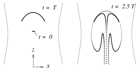
Figure 10: Plot of a particle cloud released at the center of the throat, for the conditions of figure 9 and $\omega=0.5$.

7 Conclusion

The conclusions of this paper are valid for passive isolated tiny heavy low-Re particles with a response time much smaller than the flow time scales, and a terminal velocity of the order of the flow velocity. For such inclusions, sedimentation effects appear in the leading-order dynamics, whereas particle inertia can be treated as a perturbation, together with the flow unsteadiness. This enables to write the particle dynamics as a non-dissipative system submitted to a dissipative perturbation.

Elliptic Stommel cells in steady plane or axisymmetric flows have been shown to occur as soon as the basic flow has an upward streamline displaying a strict local maximum with peak velocity $V_{c}$, and for heavy Stokes particles such that $V_{T}<V_{c}$ and $V_{T}$ close enough to $V_{c}$, in the limit of vanishing particle inertia. These results are not really new, as many authors already observed particle trapping in the vicinity of upward streamlines [5] [6] [7] [8]. However, the calculations of the present paper confirm that elliptic Stommel cells can form in a wide variety of flows, and do not require the flow to have closed streamlines or stagnation points. In particular, they can appear also if the basic flow is an open flow, like the vertical pipe flow with varying radius investigated above.

When the flow is submitted to a weak time-periodic perturbation, the separatrices of these cells can be broken (heteroclinic bifurcation) and chaotic trapping, as well as chaotic trajectories, can occur. The parameters leading to separatrix splitting have been calculated in the case where only the quadratic non-linearities of the fluid velocity field can be taken into account (i.e. ${\cal R}$ is zero or negligible). We have shown that particle inertia prevents the appearance of chaotic dynamics in the present case, by inducing an additive constant $-k\,m$ into the Melnikov function $M(t_{0})$. Therefore, particle inertia tends to maintain the stable and unstable manifolds W^s and W^u far from each other. This is clearly a centrifugal effect, since the constant part of the Melnikov function is mainly an integral of the curvature of the separatrix. In contrast, the flow unsteadiness tends to make the manifolds intersect, and the most dangerous perturbation frequency is the peak frequency of the Fourier transform of a combination of the coordinates of the point $\vec{X}_{0}(t)$ running on the separatrix. This combination depends on the detailed shape of the perturbation. The analytical expression of $M(t_{0})$ provides efficient criteria to predict the occurrence of chaos. These criteria have been tested by means of numerical computations, and the agreement is satisfactory : when $\psi^{0}$ is a cubic function of position (${\cal R}=0$) chaotic trapping is observed only if the Melnikov analysis predicts separatrix splitting. The agreement is also satisfactory if ${\cal R}$ is non-zero but decays faster than $\mid\vec{x}-\vec{x}_{c}\mid^{5}$ provided $\mid V_{T}-V_{c}\mid$ is small enough.

The Melnikov function $M(t_{0})$ of the vertical separatrix $\Sigma_{2}$ has no constant part : $m(V_{T})=0$ for all $V_{T}$. Furthermore, for the homothetic perturbation (13) we have $M(t_{0})=0$ for all $t_{0}$, so that the first-order Melnikov analysis is not conclusive there. In contrast, other kinds of perturbations, like periodical rotation around C or translation, lead to Melnikov functions of the form $M(t_{0})=A(\omega,V_{T})\sin(\omega t_{0}+\phi)$ which enable to conclude that $\Sigma_{2}$ is also splitted : this leads to extremely efficient mixing properties which could be of interest, for example, in microfluidic devices. Indeed, if the three separatrices break, particles released in the right-hand-side half-plane ($x>0$) could penetrate into the cell and get mixed with particles initially located in the left-hand-side half-plane ($x<0$).

As noted before, the elliptic cells, like the heteroclinic bifurcation, can occur in a wide variety of flows. We have checked that if the basic flow is itself an elliptic dipole (like Hadamard cells within a bubble) with center C, then particle trajectories can take the form of a smaller elliptic dipole centred at C. When this basic flow is submitted to a time periodic perturbation, separatrices can be broken and particles can have complex trajectories within the dipole : some remain trapped in the Stommel cell, and some exit the cell and drop to the bubble interface. This model can be applied to dust transport within a drop or a bubble, a topic of interest in process engineering, and could help calculate bubble contamination rates. Also, for inner Hadamard cells or Hills’ vortex one can check that ${\cal R}\equiv 0$, so that the Taylor expansion of the Hamiltonian $H$ is exact there, and the undergoing analytical results are particularly accurate.

Finally, for non-heavy particles, buoyancy and pressure gradient and added mass can be readily taken into account in the particle motion equation. This leads to interesting particle behaviours which are currently under study. Also, Basset’s drag correction, manifesting the effect of the unsteadiness of the disturbance flow due to the particle, could influence the particle dynamics and the occurrence of separatrix splitting. One can check that this correction induces an $O(\varepsilon^{3/2})$ integral term into the asymptotic motion equation (2) (see also Druzhinin & Ostrovsky [14]). This time integral makes the analysis much more complicated, and little results are available there. Note however that first-order fluid inertia effects, responsible for lift or drag corrections, should also be taken into account, since the Stokes number of the inclusion (measuring the unsteadiness of the particle-induced flow) is often of the order of its Taylor number (which characterizes first-order fluid inertia effects). Unfortunately, no general particle motion equation is available in this case, and the dynamics of such inclusions remains an open issue.

Acknowledgement The author wishes to thank J.-P. Brancher for stimulating discussions about fluid dynamics and dynamical systems. Remarks from scientists of the Fluid Dynamics group of LEMTA are gratefully acknowledged.

Appendix A Calculation of the Melnikov function

The calculation of the complete integral (10) requires to solve the differential equation

$$\vec{\dot{X}}_{0}=\vec{V}_{f}^{0}(\vec{X}_{0}(t))+\vec{V}_{T},$$ (19)

with $\vec{X}_{0}(-\infty)=A$ and $\vec{X}_{0}(+\infty)=B$. Also, $\vec{X}_{0}(t)$ belongs to the curved separatrix, so

$$\alpha(x_{0}(t)-x_{c})^{2}+\gamma(y_{0}(t)-y_{c})^{2}+\delta=0,$$

where $\vec{X}_{0}=(x_{0},y_{0})$. Therefore, the vertical coordinate of $\vec{X}_{0}$ satisfies :

$$\dot{y}_{0}=-\frac{\partial H}{\partial x}=2\alpha(x_{0}(t)-x_{c})^{2}=-2\Big{(}\gamma(y_{0}(t)-y_{c})^{2}+\delta\Big{)},$$

and the solution of this elementary equation, with $y_{0}(\pm\infty)=y_{c}\mp b$ and $y_{0}(0)=y_{c}$, is $y_{0}(t)=y_{c}-b\,\tanh(2\gamma\,b\,t)$ where $b=\sqrt{-\delta/\gamma}$. We readily obtain the horizontal coordinate of $\vec{X}_{0}(t)$ : $x_{0}(t)=x_{c}+a/\cosh(2\gamma\,b\,t),$ where $a=\sqrt{-\delta/\alpha}$. The constant part of the Melnikov function is therefore

$$m=\int_{-\infty}^{+\infty}(\dot{x}_{0}\ddot{y}_{0}-\ddot{x}_{0}\dot{y}_{0})\,dt$$

$$=-4ab^{3}\gamma^{2}\int_{-\infty}^{+\infty}\frac{ds}{\cosh^{3}s}=-2\pi ab^{3}\gamma^{2}.$$

By writing $a$, $b$ and $\gamma$ in terms of $V_{c}$, $V_{T}$ and $\psi^{0}$ we are led to expression (12).

The Melnikov integral corresponding to the homothetic perturbation (13), by using (19), reads :

$$M(t_{0})=\int_{-\infty}^{+\infty}\vec{\dot{X}}_{0}\wedge\vec{V}_{f}^{0}\Big{(}\vec{X}_{0}(t)\Big{)}\sin\omega(t+{t_{0}})\,dt-k\,m.$$

Using once again (19) :

$$M(t_{0})=-\int_{-\infty}^{+\infty}\vec{\dot{X}}_{0}\wedge\vec{V}_{T}\,\sin\omega(t+{t_{0}})\,dt-k\,m$$

$$=\mbox{Im}\,V_{T}\,e^{i\omega t_{0}}\,\int_{-\infty}^{+\infty}\dot{x}_{0}(t)e^{i\omega t}\,dt-k\,m,$$

where Im denotes the imaginary part and $\vec{V}_{T}=-V_{T}\,\vec{e}_{y}$. By inserting the analytical expression of $x_{0}(t)$ into this Fourier integral we are led to :

$$\int_{-\infty}^{+\infty}\dot{x}_{0}(t)e^{i\omega t}\,dt=\frac{1}{2i}\frac{\pi a\omega}{b\gamma}\frac{1}{\cosh(\pi\omega/4b\gamma)},$$

and this leads to $M(t_{0})=-A(\omega,V_{T})\cos\omega t_{0}-k\,m(V_{T})$, with $A(\omega,V_{T})$ given by (14).

Appendix B Lower bound for $V_{T}$ leading to heteroclinic bifurcation

In this appendix we make use of the Melnikov function $M(t_{0})$ to derive an analytical expression of the range of terminal velocities $V_{T}$ for which the heteroclinic bifurcation does not occur. By using (14) we obtain a necessary condition for the existence of both the elliptic structure and simple zeros in $M(t_{0})$ :

$$V_{c}-D(\psi^{0})<V_{T}<V_{c},$$ (20)

where $D(\psi^{0})$ is :

$$D(\psi^{0})=\frac{s^{2}}{3}-\frac{6s^{2}V_{c}-s^{4}}{3D_{1}^{1/3}}+\frac{D_{1}^{1/3}}{3}$$ (21)

and $D_{1}=D_{1}(\psi^{0})$ is given by :

$$D_{1}(\psi^{0})=$$

$$27V_{c}^{2}s^{2}/2-9V_{c}s^{4}+s^{6}+\frac{3}{2}\sqrt{81V_{c}^{4}s^{4}-12V_{c}^{3}s^{6}}$$ (22)

and

$$s=\frac{\kappa\sqrt{2}}{k\pi\sqrt{\psi^{0}_{,xyy}\mbox{\small(C)}}},$$ (23)

and $\displaystyle{\kappa=\max_{q}\frac{q}{\cosh q}\simeq 0.663}$. To obtain this result we rewrite (14) as

$$A(\omega,V_{T})=\frac{2\sqrt{6}\,V_{T}}{\sqrt{\psi^{0}_{,xxx}}}\sqrt{V_{c}-V_{T}}\,\,F\Big{(}\frac{\pi\,\omega}{2\sqrt{2}\sqrt{\psi^{0}_{,xyy}(V_{c}-V_{T})}}\Big{)}$$ (24)

with $F(q)=q/\cosh q$. One can easily check that $F$ is a bounded function with $\displaystyle{\kappa=\max_{q}\frac{q}{\cosh q}\simeq 0.663}$. Hence, whatever $\omega$ the function $F$ in (24) is at most equal to $\kappa$, so that condition

$$\frac{2\sqrt{6}\,V_{T}}{\sqrt{\psi^{0}_{,xxx}}}\sqrt{V_{c}-V_{T}}\,\,\kappa<k\,\mid m(V_{T})\mid\,\,$$

implies that $M(t_{0})$ does not have any zero. By taking the square of this inequality, which only involves positive quantities, we are led to a condition of the form $P_{3}(V_{T})>0$ where $P_{3}(X)=(V_{c}-X)^{3}-s^{2}\,X^{2}$ is a 3rd order polynomial, and $s$ is given by (23). One can easily check that $P_{3}$ is a decaying function of $X$, for all $X\geq 0$, and that $P_{3}(0)=V_{c}^{3}>0$ and $P_{3}(V_{c})=-s^{2}\,V_{c}^{2}<0$ : $P_{3}$ has a real root somewhere between 0 and $V_{c}$. If $V_{T}$ is smaller than this root, then $P_{3}(V_{T})>0$ and $M(t_{0})$ does not have any zero. An analytical expression of the root can be found by solving $P_{3}$ and we are led to $V_{T}<V_{c}-D(\psi^{0})$ with $D(\psi^{0})$ given by Eqs. (21)-(22). This is a sufficient condition for non-chaotic sedimentation. The opposite of this condition provides a necessary condition for the heteroclinic tangle to occur. In the three dimensional axisymmetric case the same method can be applied, starting from the Melnikov function given by (17) and (18). We are led to the same polynomial $P_{3}$, so that formulas (21) - (22) can be applied, but with a different value for $s$ :

$$s=\frac{3\kappa}{2\pi k\sqrt{f_{,zz}\mbox{\small(C)}}},$$ (25)

and $\displaystyle{\kappa=\max_{q\geq 0}\frac{q^{2}}{\sinh q}\simeq 1.1046}$. Finally, note that all these formulas are valid if ${\cal R}\equiv 0$.

Appendix C Effect of the remainder of the streamfunction

The particle dynamics (2) can be written as :

$$\vec{\dot{X}}_{p}=\vec{V}_{T}+\vec{V}_{f}^{0}(\vec{X}_{p})$$

$$+{\varepsilon\Big{(}\vec{V}_{f}^{1}(\vec{X}_{p},t)-k\,\overline{\overline{\nabla}}\vec{V}_{f}^{0}.(\vec{V}_{f}^{0}+\vec{V}_{T})\Big{)}}+O(\varepsilon^{2})$$ (26)

with

$$\vec{V}_{T}+\vec{V}_{f}^{0}=\left(\begin{array}[]{r}\frac{\partial H}{\partial y}\\ -\frac{\partial H}{\partial x}\end{array}\right).$$

The Taylor expansion (8) of the particle streamfunction is of the form $H(x,y)=H_{3}(\vec{x}-\vec{x}_{c})+{\cal R}(\vec{x}-\vec{x}_{c}),$ where $H_{3}$ is a third-order polynomial function of $\vec{x}-\vec{x}_{c}$ and ${\cal R}$ is a $q$-th order function of $\vec{x}-\vec{x}_{c}$ with $q\geq 4$. The inertialess particle velocity is therefore affected by the remainder :

$$\vec{V}_{T}+\vec{V}_{f}^{0}=\underbrace{\left(\begin{array}[]{r}\frac{\partial H_{3}}{\partial y}\\ -\frac{\partial H_{3}}{\partial x}\end{array}\right)}_{\vec{V}_{2}}+\underbrace{\left(\begin{array}[]{r}\frac{\partial{\cal R}}{\partial y}\\ -\frac{\partial{\cal R}}{\partial x}\end{array}\right)}_{\vec{W}_{q-1}}$$

where $\vec{V}_{2}$ is of order 2 and $\vec{W}_{q-1}$ is of order $q-1$ in $\vec{x}-\vec{x}_{c}$. The particle motion equation (26) therefore reads :

$$\vec{\dot{X}}_{p}=\vec{V}_{2}+\varepsilon\Big{(}\vec{V}_{f}^{1}(\vec{X}_{p},t)-k\overline{\overline{\nabla}}\vec{V}_{2}.\vec{V}_{2}\Big{)}+\Big{[}\underbrace{\vec{W}_{q-1}}_{(i)}$$

$$-k\underbrace{\varepsilon(\overline{\overline{\nabla}}\vec{V}_{2}.\vec{W}_{q-1}+\overline{\overline{\nabla}}\vec{W}_{q-1}.\vec{V}_{2}+\overline{\overline{\nabla}}\vec{W}_{q-1}.\vec{W}_{q-1})}_{(ii)}\Big{]}$$ (27)

where all the terms within the brackets are induced by ${\cal R}$ and have to be negligible compared to the other terms. When $\vec{x}$ is in the vicinity of the ellipse we have $\mid\vec{x}-\vec{x}_{c}\mid=O(\max(a,b))=O(\mid\delta\mid^{1/2})$, since both $\psi^{0}_{,xxx}(C)$ and $\psi^{0}_{,xyy}(C)$ in Eq. (7) are $O(1)$. Therefore, in the vicinity of the ellipse we have :

$$\vec{W}_{q-1}=O\Big{(}\mid\delta\mid^{(q-1)/2}\Big{)}\ll\vec{V}_{2}=O\Big{(}\mid\delta\mid\Big{)},$$

$$\overline{\overline{\nabla}}\vec{V}_{2}.\vec{W}_{q-1}=O\Big{(}\mid\delta\mid^{q/2}\Big{)}\ll\overline{\overline{\nabla}}\vec{V}_{2}.\vec{V}_{2}=O\Big{(}\mid\delta\mid^{3/2}\Big{)}$$

as soon as $\mid\delta\mid\ll 1$. Therefore the particle inertia term $\varepsilon\overline{\overline{\nabla}}\vec{V}_{2}.\vec{V}_{2}$ dominates all the terms in $(ii)$. Most importantly, the particle inertia term $\varepsilon\overline{\overline{\nabla}}\vec{V}_{2}.\vec{V}_{2}$ also dominates the spurious term $(i)$ provided $k\varepsilon\mid\delta\mid^{3/2}$ dominates $\mid\delta\mid^{(q-1)/2}$, i.e.

$$k\varepsilon\gg\,\mid\delta\mid^{(q-4)/2}.$$

This condition is satisfied if $q>4$ and if $\delta$ is sufficiently small. (This conclusion could have also been obtained by normalizing $(x,y)$ by $(x/\mid\delta\mid^{1/2},y/\mid\delta\mid^{1/2})$ in the particle motion equation.) In the flow $\psi^{0}=\sin x\sin y$ used here we have $q=5$, and this allows us to neglect the effect of the bracketted terms of Eq. (27) provided $\delta$ is small enough. The numerical calculations presented here show that $\delta$ does not need to be very small.

References

- [1] G.T. CSANADY. Turbulent diffusion of heavy particles in the atmosphere. J. Atmos. Sci., 20:201–208, 1963.
- [2] W.H. SNYDER and J.L. LUMLEY. Some measurements of particle velocity autocorrelation functions in a turbulent flow. J. Fluid Mech., 48:47–71, 1971.
- [3] M. R. MAXEY. The gravitational settling of aerosol particles in homogeneous turbulence and random flow fields. J. Fluid Mech., 174:441–465, 1987.
- [4] H. BENARD. Les tourbillons cellulaires dans une nappe liquide. Rev. Gen. Sci. Pure Appl., 11:1261, July 1900.
- [5] H. STOMMEL. Trajectories of small bodies sinking slowly through convection cells. J. Marine Res., 8:24–29, 1949.
- [6] B. SIMON and Y. POMEAU. Free and guided convection in evaporating layers of aqueous solutions of sucrose. transport and sedimentation of particles. Phys. Fluids A, 3:380–384, 1991.
- [7] P. CERISIER, B. PORTERIE, A. KAISS, and J. CORDONNIER. Transport and sedimentation of solid particles in Bénard hexagonal cells. Eur. Phys. J. E, 18:85–93, 2005.
- [8] I. TUVAL, I. MEZIC, F. BOTTAUSCI, Y.T. ZHANG, N. MAC DONALD, and O. PIRO. Control of particles in microelectrode devices. Phys. Rev. Let., 95(236002), 2005.
- [9] M. R. MAXEY and S. CORRSIN. Gravitational settling of aerosol particles in randomly oriented cellular flow fields. J. Atmos. Sci., 43(11):1112–1134, 1986.
- [10] J.C.H. FUNG. Gravitational settling of small spherical particles in unsteady cellular flow fields. J. Aerosol Sci., 5:753–787, 1997.
- [11] J. RUBIN, C.K.R.T. JONES, and M. MAXEY. Settling and asymptotic motion of aerosol particles in a cellular flow field. J. Nonlinear Sci., 5:337–358, 1995.
- [12] J.B. MACLAUGHLIN. Particle size effects on lagrangian turbulence. Phys. Fluids, 31(9):2544–2553, 1988.
- [13] J. GUCKENHEIMER and P. HOLMES. Non-linear oscillations, dynamical systems and bifurcation of vector fields. 1983. Springer.
- [14] O.A. DRUZHININ and L.A. OSTROVSKY. The influence of Basset force on particle dynamics in two-dimensional flows. Physica D, 76:34–43, 1994.