On matrix-free computation of 2D unstable manifolds

Abstract

Recently, a flexible and stable algorithm was introduced for the computation of 2D unstable manifolds of periodic solutions to systems of ordinary differential equations. The main idea of this approach is to represent orbits in this manifold as the solutions of an appropriate boundary value problem. The boundary value problem is under determined and a one parameter family of solutions can be found by means of arclength continuation. This family of orbits covers a piece of the manifold. The quality of this covering depends on the way the boundary value problem is discretised, as do the tractability and accuracy of the computation. In this paper, we describe an implementation of the orbit continuation algorithm which relies on multiple shooting and Newton-Krylov continuation. We show that the number of time integrations necessary for each continuation step scales only with the number of shooting intervals but not with the number of degrees of freedom of the dynamical system. The number of shooting intervals is chosen based on linear stability analysis to keep the conditioning of the boundary value problem in check. We demonstrate our algorithm with two test systems: a low-order model of shear flow and a well-resolved simulation of turbulent plane Couette flow.

1 Introduction

In recent years, an increasing number of algorithms from numerical dynamical systems theory have become available for systems with many degrees of freedom. These algorithms are designed for the computation and continuation of equilibrium states, time-periodic solutions, invariant tori and connecting orbits and are usually of the prediction-correction variety. The prediction can be based simply on data filtered from simulations or on extrapolation of a previously computed part of the continuation curve. The correction step, however, involves solving a large set of coupled nonlinear equations by an iterative method. Because of its quadratic convergence, the most desirable method here is Newton-Raphson iteration. This method, in turn, requires the repeated solution of a large linear system. It is not surprising, then, that the most significant step forward in this field was the introduction of Krylov subspace methods for solving the linear systems. The combination of Newton-Raphson iteration with a Krylov subspace method for prediction-correction methods is now referred to as Newton-Krylov continuation.

Newton-Krylov continuation has been used extensively in the context of fluid dynamics, where a large system of ordinary differential equations (ODEs) results from discretisation of the Navier-Stokes equation and possibly the continuity and energy equations. Early examples include the computation of equilibrium states in Taylor vortex flow by Edwards et al. [3] and the continuation of time-periodic solutions by Sánchez et al. [14]. More recently, the algorithm has also been used for the computation of quasi-periodic solutions [15].

Now that algorithms for the study of equilibria and (quasi) periodic solutions are available, it is natural to consider their stable and unstable manifolds and the global dynamical structures they represent. It is a well-known fact from dynamical systems theory that these manifolds, and the way they intersect in phase space, play an essential role in such phenomena as the generation of chaos, boundary crises and bursting behaviour. The tractability of manifold computation depends critically on the manifold dimension. A one-dimensional (un)stable manifold is just an integral curve of the ODEs and its computation is simple. The computation of manifolds of dimension three and up would be a formidable task. Even if we would design an algorithm which works regardless of the dimension of the ambient space, the representation of the manifold in a discrete data set and its interpretation would present great difficulties.

In the current paper we focus on the computation of two-dimensional invariant manifolds. A number of algorithms has been designed for this end, mostly for low-dimensional systems. An overview of methods can be found in Krauskopf et al. [9]. One method presented there is particularly suitable for adaption to high dimensional systems. This method is called orbit continuation [9, Sec. 3] and is based on a representation of the integral curves which fill the manifold as solutions to an under determined boundary value problem (BVP). Using a conventional prediction-correction method to approximate the continuous, one-parameter family of solutions to this BVP, we construct an approximation to the manifold by finitely many integral curves. Being originally designed for low-dimensional systems, this method was implemented in the BVP solver AUTO [1], which uses spectral collocation to represent the integral curves and direct methods to solve the linear equations which arise from Newton-Raphson iteration. In adapting the method to high-dimensional systems, we discard spectral collocation in favour of multiple shooting and implement Newton-Krylov continuation. Thus, we strike a compromise between control over the covering of the manifold on one hand and tractability of the algorithm on the other hand.

Two important points to consider when applying Newton-Krylov continuation are the efficiency of the Krylov subspace method and the extent to which the algorithm is parallelisable. These issues can be closely connected. A good example is given by the continuation of periodic solutions in Navier-Stokes flow. When using single shooting, the Jacobian matrix of the Newton-Raphson iteration is very well handled by Krylov subspace methods. This is because its spectrum is strongly clustered [14]. If, however, we employ the highly parallelisable multiple shooting algorithm, the eigenvalues spread out over the complex plane and preconditioning is necessary to ensure linear speedup [13]. We will show that Newton-Krylov orbit continuation with multiple shooting does not require preconditioning. In particular, we will show that the minimal dimension of the Krylov subspace scales linearly with the number of shooting intervals but does not depend on the number of ODEs.

We illustrate the algorithm with two examples. The first example is a toy model of shear flow, originally introduced by Waleffe [16]. In Sec. 6.1 we show Newton-Krylov convergence results and a comparison to AUTO computations. The second example is a well-resolved simulation of turbulent Couette flow, presented in Sec. 6.2. In this case, the high number of degrees of freedom in the simulation precludes the use of spectral collocation and direct linear solvers. In either case, we compute the unstable manifold of a periodic solution with a single unstable multiplier. This is related to an open issue in turbulent shear flow, namely the idea that certain time-periodic solutions with a two-dimensional unstable manifold play a key role in bursting behaviour [2], which formed the original motivation for this work. Nevertheless, the algorithm presented here has wider applicability. If an equilibrium state has two unstable directions, we can simply adjust the left boundary condition, as explained below. If we wish to compute a two-dimensional stable manifold, we can either reverse time or rephrase the BVP, reversing the role of the left and right boundary conditions.

2 Orbit continuation

Let us denote the system of ODEs and the associated linearised system as

$$\dot{\mathbf{x}} =\mathbf{f}(\mathbf{x})\ \ \ \text{where}\ \ \mathbf{x}\in\mathbb{R}^{n}$$ (1)

$$\dot{\mathbf{v}} =D\mathbf{f}\,\mathbf{v}$$ (2)

and let the flow of system (1) be denoted by $\phi(\mathbf{x},t)$. We assume there is a hyperbolic periodic solution passing through the point $\bar{\mathbf{x}}$, i.e. $\bar{\mathbf{x}}=\phi(\bar{\mathbf{x}},0)=\phi(\bar{\mathbf{x}},P)$, where $P$ is the period. We can write the solution to the linearised system (2) about this periodic solution as $\mathbf{v}(P)=\mathbf{M}\,\mathbf{v}(0)$, where $\mathbf{M}$ is the monodromy matrix. We assume that $\mathbf{M}$ has a single eigenvalue outside the unit circle in the complex plane, i.e. $|\mu_{n}|\leq|\mu_{n-1}|\leq\ldots\leq\mu_{2}=1\leq\mu_{1}$. Let $\mathbf{u}_{1}$ be the corresponding eigenvector based at $\bar{\mathbf{x}}$, i.e. $\mathbf{M}\mathbf{u}_{1}=\mu_{1}\mathbf{u}_{1}$. Our aim is to compute a finite piece of the two dimensional unstable manifold, tangent at $\bar{x}$ to the linear subspace spanned by $\mathbf{u}_{1}$ and $\mathbf{u}_{2}=\mathbf{f}(\bar{\mathbf{x}})$.

Orbits segments contained in this manifold, which we will denote by $\mathbf{\gamma}(t)$, approximately satisfy the following boundary condition:

$$\mathbf{\gamma}(0) =\bar{\mathbf{x}}+\epsilon\mathbf{u}_{1}$$ (left boundary condition)

$$g(\mathbf{\gamma},T) =c$$ (right boundary condition) (3)

where $g$ is a scalar function or functional. The choice of a suitable right boundary condition depends on the problem and on the goal of the computation. Common choices, which we will use throughout this paper, are

$$g(\mathbf{\gamma},T) =T$$ for orbits of fixed integration time

$$g(\mathbf{\gamma},T) =\int_{0}^{T}|\mathbf{f}(\mathbf{\gamma}(t))|\,dt$$ for orbits of constant arc length

$$g(\mathbf{\gamma},T) =g(\mathbf{\gamma}(T))$$ for orbits terminating on a Poincaré surface

The crucial observation is that this BVP is under determined by a single unknown. For a suitable choice of the right boundary condition, there exists a continuous, one parameter family of solutions which covers part of the manifold. Of course, the left boundary condition is approximate and an error is introduced for finite $\epsilon$. However, due to the exponential contraction transversal to the unstable manifold this error does not increase along $\mathbf{\gamma}(t)$.

In order to compute the two-dimensional unstable manifold of an equilibrium state, all we need to do is replace the left boundary condition. We fix a circle with a small radius in the subspace spanned by the two unstable eigenvectors and demand that the initial point lie on this circle. The free parameter is an angle [9, Sec. 3].

To see that the BVP is under determined, it is instructive to think of it as a shooting problem. Every orbit segment $\mathbf{\gamma}(t)$ is uniquely determined by its initial point and integration time. Then, the $(n+2)$ unknowns of this BVP are $T$, $\epsilon$ and the components of $\mathbf{\gamma}(0)$, whereas conditions (3) constitute $(n+1)$ equations.

A standard method to numerically approximate the family of solutions is arclength continuation. This is a prediction-correction method. Let us write BVP (3) compactly as

$$\mathbf{F}(\mathbf{z})=0\qquad\text{where}\ \mathbf{z}^{t}=(\mathbf{\gamma}(0),T,\epsilon)$$ (4)

and let $\mathbf{T}$ denote the tangent to the family of solutions. Then the basic algorithm can be summarised as follows:

Single shooting arclength continuation of BVP (3) 1. Find an initial solution by forward integration starting at $\mathbf{\gamma}(0)=\bar{\mathbf{x}}+\epsilon_{0}\mathbf{u}_{1}$ and stopping when $g(\mathbf{\gamma},T_{0})=c$. Set $\mathbf{z}_{0}^{t}=(\mathbf{\gamma}(0),T_{0},\epsilon_{0})$ and find $\mathbf{T}_{0}$. 2. Prediction: $\mathbf{z}^{0}_{i+1}=\mathbf{z}_{i}+\Delta s\,\mathbf{T}_{i}$. 3. Correction: solve $$\mathcal{A}\,\delta\mathbf{z}^{j}=\left(\begin{array}[]{c}\ D\mathbf{F}\\ \mathbf{T}_{i}^{t}\end{array}\right)\delta\mathbf{z}^{j}=-\left(\begin{array}[]{c}\mathbf{F}(\mathbf{z}_{i+1}^{j})\\ 0\end{array}\right)$$ (5) and update $\mathbf{z}_{i+1}^{j+1}=\mathbf{z}_{i+1}^{j}+\delta\mathbf{z}^{j}$ until a Newton-Raphson convergence criterion is met. Then set $\mathbf{z}_{i+1}=\mathbf{z}_{i+1}^{j}$. 4. Control step size $\Delta s$. 5. Repeat 2.-4. for $i=1,2,\ldots,i_{\rm max}$.

In order to make the Newton-Raphson correction step unique we use the condition that $\mathbf{T}_{i}\perp\delta\mathbf{z}^{j}_{i+1}$ in Eq. (5). This condition can always be met for small enough step size $\Delta s$ and does not require extra computations. As we will see below, step 4. is important because it allows us to put an upper bound on the changes to unknowns and thus, indirectly, to control the covering of the manifold.

The main factor which decides if this scheme is feasible numerically is the condition of the linear problem (5). In systems with sensitive dependence on initial conditions, the linear problem gets increasingly harder to solve as we try to compute a larger part of the manifold. This is most clearly seen if we select the right boundary condition that the end points of the segments lie in a Poincaré surface of intersection. In that case we have

$$\mathcal{A}=\left(\begin{array}[]{ccc}\mathbb{I}_{n}&\mathbf{0}&-\mathbf{u}_{1}\\ (\nabla g)^{t}D\phi&(\nabla g)^{t}\mathbf{f}&0\\ \hline\cr&\mathbf{T}^{t}&\end{array}\right)$$ (6)

where $D\phi$ and $\mathbf{f}$ are evaluated at $\gamma(T)$. It can be shown that both the 2-norm and the condition number of $\mathcal{A}$ are bound from below by $\max_{j=1\ldots n}|(\nabla g)_{i}D\phi_{ij}|$ and we can expect $\|D\phi\|$ to grow exponentially with the integration time $T$.

3 The limitations of spectral collocation

Without being rigorous, we can say that the optimal solution to the problem of sensitive dependence on initial conditions lies in the use of spectral collocation. Rather than to approach BVP (3) as a single shooting problem, we can represent the orbits $\mathbf{\gamma}(t)$ on a mesh using orthogonal basis functions. This approach is used in the widely used software package AUTO [1]. A survey of results using spectral collocation for orbit continuation can be found in Krauskopf and Osinga [8]. The main strength of this approach is that the set of unknowns includes the complete set of collocation coefficients. When we control the arclength step size, we control the change in shape of the entire orbit. Thus, we can be reasonably certain that we miss no details of the geometry of the manifold.

This control comes at a price, however. The total number of unknowns to solve for in every step will be proportional to $N_{\rm m}\times N_{\rm c}\times n$, where $N_{\rm m}$ is the number of mesh intervals and $N_{\rm c}$ is the number of collocation points per mesh interval. The minimal number of mesh intervals in turn depends on the number of mesh intervals necessary for resolving the periodic solution, $N_{\rm m}^{(0)}$, and the unstable multiplier, $\mu_{1}$. If we assume that the dynamics close to the periodic orbit is well described by the linearisation, the distance to the periodic orbit will grow as $\epsilon\mu_{1}^{p}$, where $p$ is the number of times we integrate “along” the periodic orbit. We can think of $p$ as the number of iterations of a Poincaré map. Thus, to resolve an orbit long enough to arrive an $\mbox{O}(1)$ distance away from the periodic orbit, we will need about $N_{\rm m}=-N_{\rm m}^{(0)}\ln(\epsilon)/\ln(\mu_{1})$ mesh intervals.

The result of this estimate depends very much on the details of the problem at hand. The geometry of the vector field close to the periodic orbit will determine the trade-off between the number of mesh intervals and the number of collocation points as well as the maximal value for $\epsilon$. We can, however, identify three possible settings in which the collocation approach is not tractable:

1. the number of degrees of freedom is large,

2. the unstable multiplier is very close to unity or

3. the periodic orbit has a complex shape.

In this paper, we will consider two examples in which situations 1. and 2. arise. Situation 3. might be encountered, for instance, in multiple time scale systems such as arise in neuro science.

Below, we will show that multiple shooting provides a good compromise between the accurate, but costly, collocation approach and the cheap, but unstable, single shooting approach. In particular, we will show that the three issues listed above will influence the computation time only through the time it takes to perform sufficiently accurate forward time integrations.

4 Multiple shooting

In this approach, we represent the orbit on the unstable manifold as the concatenation of $k$ segments. For each segment, we specify a scalar right boundary condition and, in addition, we have $(k-1)$ gluing conditions to ensure the resulting orbit is continuous.

Let us define the vector of $N=(k-1)n+k+1$ unknowns as

$$\mathbf{z}=(\gamma^{(2)}(0),\ldots,\gamma^{(k)}(0),\,T^{(1)},\ldots,\,T^{(k)},\,\epsilon)$$

and the set of $(N-1)$ nonlinear equations as

$$\mathbf{F}=\left(\gamma^{(2)}(0)-\gamma^{(1)}(T^{(1)}),\ldots,\gamma^{(k)}(0)-\gamma^{(k-1)}(T^{(1)}),\,g^{(1)}(\gamma^{(1)},T^{(1)})-c_{1},\ldots,\right.\\ \left.g^{(k)}(\gamma^{(k)},\,T^{(k)})-c_{k}\right)$$ (7)

We can rewrite the basic continuation algorithm for shooting on $k$ intervals as shown below. Instead of using direct methods, which require computation of the full matrix of derivatives, we can use a Krylov subspace method. In particular, we will use GMRES [12].

Multiple shooting Newton-Krylov continuation of BVP (7) 1. Find an initial solution by forward integration starting from $\mathbf{\gamma}(0)=\bar{\mathbf{x}}+\epsilon_{0}\mathbf{u}_{1}$. Set $\mathbf{T}=(0,\ldots,0,1)^{t}$. 2. Prediction: $\mathbf{z}^{0}_{i+1}=\mathbf{z}_{i}+\Delta s\,\mathbf{T}_{i}$. 3. Correction: approximate the solution to $$\mathcal{A}\,\delta\mathbf{z}^{j}=\left(\begin{array}[]{c}\ D\mathbf{F}\\ \mathbf{T}_{i}^{t}\end{array}\right)\delta\mathbf{z}^{j}=-\left(\begin{array}[]{c}\mathbf{F}(\mathbf{z}_{i+1}^{j})\\ 0\end{array}\right)$$ (8) by GMRES iterations up to tolerance $d$ and update $\mathbf{z}_{i+1}^{j+1}=\mathbf{z}_{i+1}^{j}+\delta\mathbf{z}^{j}$ until a Newton-Raphson convergence criterion is met. Then set $\mathbf{z}_{i+1}=\mathbf{z}_{i+1}^{j}$. 4. Control step size $\Delta s$. 5. Compute $\mathbf{T}$ by finite differences. 6. Repeat 2.-5. for $i=1,2,\ldots,i_{\rm max}$.

We note that this algorithm is essentially the same as that employed by Sánchez and Net [13]. Technically, the important distinction between the two algorithms is the structure of $\mathcal{A}$. In the case of continuation of periodic orbits with multiple shooting, its eigenvalues spread out in the complex plane and preconditioning is necessary to ensure that the number of GMRES iterations in the innermost loop remains small. In the manifold computation we will see that the number of GMRES iterations grows in proportion to the number of shooting intervals but is independent of $n$ even without preconditioning.

The matrix $\mathcal{A}$ has the following structure

$$\mathcal{A}=\left(\begin{array}[]{cc}\mathcal{A}^{\prime}&\mathbf{A}\\ \mathbf{B}&\mathbf{C}\end{array}\right)=\left(\begin{array}[]{cccccc|c}\mathbb{I}&&&&&&\\ -\mathbf{J}_{2}&\mathbb{I}&&&&&\\ &\ddots&\ddots&&&&\mathbf{A}\\ &&-\mathbf{J}_{k-2}&\mathbb{I}&&&\\ &&&-\mathbf{J}_{k-1}&\mathbb{I}&&\\ \hline\cr&&\mathbf{B}&&&&\mathbf{C}\\ \end{array}\right)$$ (9)

where $\mathbf{A}$ is a $(k-1)n\,\times\,(k+1)$ matrix of derivatives of the gluing conditions with respect to the integration times and the small parameter, $\mathbf{B}$ is a $(k+1)\,\times\,(k-1)n$ matrix of derivatives of the right boundary conditions with respect to the initial points complemented by the first $(k-1)n$ components of $\mathbf{T}$ and $\mathbf{C}$ is a $(k+1)\,\times\,(k+1)$ matrix of derivatives of the right boundary conditions with respect to the integration times and the small parameter complemented by the last $(k+1)$ components of $\mathbf{T}$. Their sparsity patterns are as follows:

$$A =\left(\!\begin{array}[]{cccccc}\mathbf{a}_{1}&\mathbf{0}&\cdots&\mathbf{0}&\mathbf{0}&\bar{\mathbf{a}}\\ \mathbf{0}&\mathbf{a}_{2}&\cdots&\mathbf{0}&\mathbf{0}&\mathbf{0}\\ \vdots&\vdots&\ddots&\vdots&\vdots&\vdots\\ \mathbf{0}&\mathbf{0}&\cdots&\mathbf{a}_{k-1}&\mathbf{0}&\mathbf{0}\end{array}\!\right)\quad B =\left(\!\begin{array}[]{cccc}\mathbf{0}&\mathbf{0}&\cdots&\mathbf{0}\\ \mathbf{b}_{2}&\mathbf{0}&\cdots&\mathbf{0}\\ \mathbf{0}&\mathbf{b}_{2}&\cdots&\mathbf{0}\\ \vdots&\vdots&\ddots&\vdots\\ \mathbf{0}&\mathbf{0}&\cdots&\mathbf{b}_{k}\\ \mathbf{t}_{1}&\mathbf{t}_{2}&\cdots&\mathbf{t}_{k-1}\end{array}\!\right)$$ (20)

$$C =\left(\!\begin{array}[]{ccccc}c_{11}&0&\cdots&0&\bar{c}\\ 0&c_{22}&\cdots&0&0\\ \vdots&\vdots&\ddots&\vdots&\vdots\\ 0&0&\cdots&c_{kk}&0\\ t_{1}&t_{2}&\cdots&t_{k}&t_{k+1}\end{array}\!\right)$$ (26)

Here, $\bar{\mathbf{a}}$ and each $\mathbf{a}_{i}$ is a column vector with $n$ elements and each $\mathbf{b}_{i}$ and $\mathbf{t}_{i}$ is a row vector with $n$ elements. Because of the partitioning of $\mathcal{A}$, it is useful to introduce the notation

$$\mathbf{v}=(\mathbf{v}^{(1)},\mathbf{v}^{(2)})^{t}=(\mathbf{v}_{1}^{(1)},\ldots,\mathbf{v}_{k-1}^{(1)},v_{1}^{(2)},\ldots,v_{k+1}^{(2)})^{t}$$

where each $\mathbf{v}_{i}^{(1)}$ is a column vector with $n$ entries and each $v^{(2)}_{i}$ is a scalar.

In order to establish the upper bound on the number of GMRES iterations we need the following lemma.

Lemma 1.

Matrix $\mathcal{A}$ has eigenvalue $\lambda_{0}=1$ with algebraic multiplicity at least $(k-1)(n-1)$ and geometric multiplicity at least $(n-1)$

Proof.

We will show that a minimal set of $(n-1)$ linearly independent eigenvectors exists for eigenvalue $\lambda_{0}$ irrespective of the choice of boundary conditions. We label these eigenvectors $\mathbf{w}_{1,i}$ ($i=1,\ldots,n-1$). Additional eigenvectors appear for each boundary condition given by constant integration time and possibly at isolated points on the continuation curve. Each of the eigenvectors in the minimal set has a preimage under $(\mathcal{A}-\mathbb{I})^{s}$ for $s=1,\ldots,k-2$. We label the generalised eigenvectors $\mathbf{w}_{s,i}$ so that

$$(\mathcal{A}-\mathbb{I})\mathbf{w}_{s+1,i} =\mathbf{w}_{s,i}\ \text{for}\ s=1,\ldots,k-2$$ (27)

$$(\mathcal{A}-\mathbb{I})\mathbf{w}_{1,i} =0$$ (28)

To prove this we use induction on $s$. In the induction step we must prove the existence of a generalised eigenvector $\mathbf{w}_{s+1,i}$ going on the equation which $\mathbf{w}_{s,i}$ satisfies. For this end we use Fredholm’s alternative. Thus, we first examine the left null space of the operator and introduce some notation that helps exploit the sparsity patterns of the (generalised) eigenvectors.

Let $R_{q}$ denote the linear subspace of vectors with the following sparsity pattern

$$\mathbf{v}=(\mathbf{0},\ldots,\mathbf{0},\mathbf{v}_{k-q}^{(1)},\ldots,\mathbf{v}_{k-1}^{(1)},0,\ldots,0,v_{k+1-q}^{(2)},\ldots,v_{k}^{(2)},0)^{t}$$

for $q=1,\ldots,k-1$. Also, let $L$ denote the linear subspace of vectors with the following sparsity pattern

$$\mathbf{v}=(\mathbf{v}_{1}^{(1)},\mathbf{0},\ldots,\mathbf{0},v_{1}^{(2)},0,\ldots,0)^{t}$$

and note that $R_{1}\subset R_{2}\subset\ldots\subset R_{k-1}$ and $L\perp R_{q}$ for $q=1,\ldots,k-2$.

First, we will assume that the functions $g^{(i)}$ which determine the right boundary conditions depend on the initial condition $\gamma^{(i)}(0)$ on each shooting interval. This is the case for right boundary conditions given by Poincaré planes of intersection or constant arclength. The case in which one or more right boundary conditions are given by constant integration time is discussed at the end of the proof.

Under this condition, the null space of $(\mathcal{A}-\mathbb{I})^{t}$ is spanned by vectors $\mathbf{v}\in L$ for which

$$\mathbf{a}_{1}\cdot\mathbf{v}_{1}^{(1)}+(c_{11}-1)v_{1}^{(2)} =0\qquad \bar{\mathbf{a}}\cdot\mathbf{v}_{1}^{(1)}+\bar{c}v_{1}^{(2)} =0$$ (29)

Note, that these conditions are linearly independent because $\mathbf{a}_{1}$ and $\bar{\mathbf{a}}$ are transversal. They correspond to variations of the final point of the first shooting segment resulting from variation in $T^{(1)}$ and $\epsilon$. These variations are the image under the nonsingular matrix $\mathbf{J}_{1}$ of $\mathbf{f}(\bar{\mathbf{x}}+\epsilon\mathbf{u}_{1})$ and $\mathbf{u}_{1}$, which are transversal for sufficiently small $\epsilon$ because in the limit of $\epsilon\downarrow 0$ they are eigenvectors of the monodromy matrix of the periodic orbit for distinct eigenvalues. Thus, we have $\text{dim}(L)-2=(n-1)$ left null vectors contained in $L$.

We now construct $(n-1)$ eigenvectors contained in $R_{1}$. Let

$$R_{1}\ni\mathbf{w}_{1,i}=(\mathbf{0},\ldots,\mathbf{v}_{k-1}^{(1)},0,\ldots,v_{k}^{(2)},0)^{t}$$ (30)

then Eq. (28) gives

$$\mathbf{b}_{k}\cdot\mathbf{v}_{k-1}^{(1)}+(c_{kk}-1)v_{k}^{(2)} =0 \qquad\mathbf{t}_{k-1}\cdot\mathbf{v}_{k-1}^{(1)}+t_{k}v_{k}^{(2)} =0$$ (31)

so that the number of eigenvectors is at least $\text{dim}(R_{1})-2=n-1$. An extra eigenvector may exist at isolated points on the continuation curve where the two condition are linearly dependent. We defer a discussion of such special points to the end of this proof. This concludes the proof for $k=2$.

For $k=3$ it suffices to note that, since $R_{1}\perp L$, Eq. (27) has a solution to each $i=1,\ldots,n-1$ by Fredholm’s alternative. In this case there are $(n-1)$ linearly independent eigenvectors and $(n-1)$ linearly independent generalised eigenvectors.

For $k>3$ we use induction on $s$. Suppose that a generalised eigenvector $\mathbf{w}_{s,i}\in R_{s}$ exists for $s<k-1$. Then it has a preimage under $(\mathcal{A}-\mathbb{I})$ by Fredholm’s alternative. We need to show that this preimage has a non-empty intersection with $R_{s+1}$. Let $\mathbf{w}_{s+1,i}=(\mathbf{v}_{1}^{(1)},\ldots,\mathbf{v}_{k-1}^{(1)},v_{1}^{(2)},\ldots,v_{k+1}^{(2)})^{t}$. The condition that $(\mathcal{A}-\mathbb{I})\mathbf{w}_{s+1,i}\in R_{s}$ gives

$$v_{1}^{(2)}\mathbf{a}_{1}+v_{k+1}^{(2)}\bar{\mathbf{a}} =0 \qquad(c_{11}-1)v_{1}^{(2)}+\bar{c}v_{k+1}^{(2)} =0$$ (32)

from which we find $v_{1}^{(2)}=v_{k+1}^{(2)}=0$. Next, we have

$$-\mathbf{J}_{i}\mathbf{v}_{i-1}^{(1)}+v_{i}^{(2)}\mathbf{a}_{i} =-\mathbf{J}_{i}\mathbf{v}_{i-1}^{(1)}-v_{i}^{(2)}\mathbf{f}(\gamma^{(i)}(T^{(i)}))=0$$ (33)

$$\mathbf{b}_{i}\cdot\mathbf{v}_{i-1}^{(1)}+(c_{ii}-1)v_{i}^{(2)} =0$$ (34)

for $i=2,\ldots,k-s-1$. The most general solution of Eq. (33) is $\mathbf{v}_{i-1}^{(1)}=\alpha\mathbf{f}(\gamma^{(i)}(0))$, $v_{i}^{(2)}=-\alpha$. The second equation depends on the $i^{\rm th}$ boundary condition. If the boundary condition is a Poincaré plane of intersection, then $\mathbf{b}_{i}=(\nabla g_{i})^{t}\mathbf{J}_{i}$ and $c_{ii}=(\nabla g_{i})^{t}\mathbf{f}(\gamma^{(i)}(T^{(i)}))=-(\nabla g_{i})^{t}\mathbf{a}_{i}$ and it follows that $\mathbf{w}_{i-1}=\mathbf{0}$ and $w_{i}^{(1)}=0$. If the right boundary condition is given by constant arc length, a solution with $\alpha\neq 0$ exists only if $\|\mathbf{f}(\gamma^{(i)}(0))\|=1$. At isolated points on the continuation curve where this holds, an extra eigenvector for $\lambda_{0}$ exists. This situation is discussed at the end of the proof. In the generic case, the conclusion is that any vector in the preimage of $\mathbf{w}_{s,i}$ is contained in $R_{s+1}$. This completes the proof, with the exception of the special cases discussed below.

For each right boundary condition given by constant integration time, an extra eigenvector for eigenvalue $\lambda_{0}$ exists. In particular, if $g^{(i)}=T^{(i)}$ for $i>1$ then there is a right eigenvector $\mathbf{z}\in R_{k+1-i}$ and a left eigenvector $\mathbf{e}_{(k-1)n+i}$, i.e. the $([k-1]n+i)^{\rm th}$ unit direction vector. It is straightforward to see that $\mathbf{e}^{t}_{(k-1)n+i}\mathbf{z}\neq 0$ so that this eigenvector does not have any generalised eigenvectors associated with it. The proof by induction for the other (generalised) eigenvectors still holds. The only difference is that if we consider Eq. (27) in the induction step we find that the preimage of $\mathbf{w}_{s,i}$ is not contained in $R_{s+1}$. However, its intersection with $R_{s+1}$ is non-empty. If $g^{(1)}=T^{(1)}$ then no additional eigenvector exists. Instead, one of the eigenvectors in the minimal set has an additional preimage.

In the exceptional cases that Eqs. (31) are linearly dependent or that Eqs. (33)-(34) allow for a nonzero solution, an additional eigenvector exists. These cases are treated just like the appearance of an additional eigenvector discussed above. Again, it is straightforward to show that the preimage of each generalised eigenvector $\mathbf{w}_{s,i}$ intersects the right subspace $R_{s+1}$. ∎

Of course, the discussion of the special cases which arise only at isolated points on the continuation curve is somewhat academic, as we will compute a discrete approximation to this curve. It is good to know, however, that no drastic changes in the eigenspectrum of $\mathcal{A}$ occur. As we will see in the following proposition, this guarantees that a global maximum for the number of GMRES iterations can be computed a priori.

Proposition 2.

Assume that all eigenvalues of $\mathcal{A}$ other than $\lambda_{0}=1$ are simple. Then the number of GMRES iterations necessary to solve (8) is at most $(3k-1)$ with exact arithmetic.

Proof.

First, assume that the right boundary conditions depend on the initial conditions on each shooting interval. Then, by Lemma 1, $\mathcal{A}$ has the Jordan normal form

$$\mathcal{A}_{\rm J}=\mathbf{Q}\mathcal{A}\mathbf{Q}^{-1}=\left(\begin{array}[]{cccccc}\mathbf{M}&&&&&\\ &\ddots&&&&\\ &&\mathbf{M}&&&\\ &&&\lambda_{1}&&\\ &&&&\ddots&\\ &&&&&\lambda_{2k}\end{array}\right)$$

where $\mathbf{M}$ is a Jordan block of dimension $(k-1)$ such that $(\mathbf{M}-\mathbb{I})^{k-1}=\mathbf{0}$. After $p$ GMRES iterations with the initial vector $\mathbf{w}$, the residue is bound from above by

$$\min_{P_{p}(0)=1}\|P_{p}(\mathcal{A})\mathbf{w}\|=\min_{P_{p}(0)=1}\|\mathbf{Q}^{-1}P_{p}(\mathcal{A}_{\rm J})\mathbf{Q}\mathbf{w}\|\leq\kappa(\mathbf{Q})\|\mathbf{w}\|\min_{P_{p}(0)=1}\|P_{p}(\mathcal{A}_{\rm J})\|$$

where the minimum is taken over all polynomials of order $p$ which satisfy $P_{p}(\mathbf{0})=\mathbb{I}$. Then we have

$$P_{3k-1}(\mathcal{A}_{\rm J})=\frac{(-1)^{k-1}}{\Pi_{i=1}^{2k}\lambda_{i}}(\mathcal{A}_{\rm J}-\mathbb{I})^{k-1}\Pi_{i=1}^{2k}(\mathcal{A}_{\rm J}-\lambda_{i}\mathbb{I})=\mathbf{0}$$

As $P_{3k-1}$ is a polynomial of order $3k-1$ this proves the proposition.

For every right boundary condition independent of the initial condition one of the simple eigenvalues is equal to $\lambda_{0}$. Thus, for each of these we can omit one GMRES iteration. The only exception is the first shooting interval. If the first boundary condition is independent of the initial condition, in that case meaning independent of variation of $\epsilon$, we have one less simple eigenvalue different from $\lambda_{0}$, but one of the Jordan blocks is of dimension $k$, so that the minimal number of iterations is $3k-1$. ∎

5 Implementation and parallelism

The Newton-Krylov continuation algorithm is easy to parallelise. For each iteration of GMRES we need to compute the matrix-vector product $\mathcal{A}\mathbf{v}$ for some given perturbation vector $\mathbf{v}$. The constituents of this product are found by integrating the extended system (1-2) on each of the shooting intervals. These integrations are all independent and can be executed on different CPUs. The matrix-vector product is then formed by the root process. This step involves only $\mbox{O}(N)$ elementary operations and the communication of vectors of length $n$. Consequently, the overhead is very small and the examples below show nearly $100\%$ efficiency of the parallelisation.

In the first example, the set of ODEs is only of dimension $17$ and the essential loop of the code is easily parallelised with openMP. In the second example, each integration is done by a pseudo-spectral Navier-Stokes simulation code [5]. In this case, distributed memory MPI parallelisation is employed.

We need to make two remarks about the stability of the algorithm. Firstly, it is more stable to use a logarithmic scale for the small parameter, i.e. $\delta=\ln(\epsilon)$. If, in addition, we normalise the integration times by the period of the unstable periodic orbit, the dependent variables in the continuation are of comparable size - assuming that the phase space variables are suitably scaled. Secondly, the matrix $\mathcal{A}$ is ill-conditioned. The condition number can be expected to increase exponentially with the integration time on each shooting interval. As a consequence, the orthogonalisation of the basis of the Krylov subspace can be unstable. This problem is largely solved by using a $QR$-decomposition based on Householder transformations.

The third remark concerns the left boundary condition in the BVP (3). In order to improve the accuracy of the manifold computation we can add a second order term to its local approximation. Using a higher order approximation, we can generally allow for larger values of $\epsilon$ in the continuation. To compute the second order term, we need to integrate the second order variational equations along the periodic orbit. This is not normally feasible for high-dimensional systems.

Finally, if the system under consideration has a strong dependence on initial conditions, we must start the continuation with a short orbit obtained by forward time integration. We can choose a Poincaré plane which intersects with the periodic orbit for a right boundary condition and let the integration time increase in the arclength continuation, adding shooting intervals when necessary. When the computed orbit is long enough, we can switch to a different boundary condition. The flexibility of the algorithm to select different parts of the manifold for computation by selecting different boundary conditions is one of its main strengths.

6 Example computations

In the following section we will describe test computations with a toy model as well as a full-fledged simulation of turbulent shear flow. In both models, there exists a periodic solution which seems to organise the phenomenon of bursting. In a bursting flow, we see turbulent episodes, during which the fluid motion is highly complex, interspersed with nearly laminar episodes, during which the motion is smooth. The periodic solution of interest has a single unstable multiplier and as a consequence its stable manifold separates the phase space [6]. Special solutions like this are sometimes called edge states [2]. In the simplest explanation of bursting, the phase point is attracted to the edge state during the laminarisation, then moves away from the edge state along a two-dimensional unstable manifold during the bursting phase. Complete laminarisation will not occur because the domain of attraction of the laminar flow is bounded by the stable manifold of the edge state. Computation of the unstable manifold we will give information about the transition from a near-laminar configuration to a turbulent one.

6.1 A low-order model of shear flow: weak instability

For the first example computation we use a model for shear flow originally introduced by Waleffe [16]. The model is obtained as a Galerkin truncation of the Navier-Stokes equation for an incompressible fluid trapped between two infinite, parallel plates with free slip boundary conditions. Energy is input by a sinusoidal body force and Fourier modes are used in all directions. Waleffe formulated this model to demonstrate the regeneration cycle in shear flows, i.e. the repeated formation and breakdown of stream wise vortices and low velocity streaks. Accordingly, the modes retained in the Galerkin truncation were chosen to have the spatial symmetries of stream wise vortices, streaks and streak instabilities. In the original paper [16], the maximal wave number was set to $2$ in the wall-normal direction and $1$ in the stream wise and span wise directions. Here, we consider maximal wave numbers $3$ and $1$, respectively, which leads to a set of $17$ nonlinear, coupled ODEs.

Obviously, such a severe truncation can only be regarded as a toy model of shear flow. Remarkably though, the low-order model has many of the qualitative traits that make shear flow so challenging from a dynamical systems point of view. First of all, there exists a linearly stable laminar solution for all Reynolds number. Secondly, for high Reynolds numbers, solutions to the ODE typically show chaotic bursts interspersed with smooth behaviour. The model introduced by Waleffe has often been used as a test case for new ideas and algorithms for parsing turbulent bursting, see e.g. Moehlis et al. [11] and references therein.

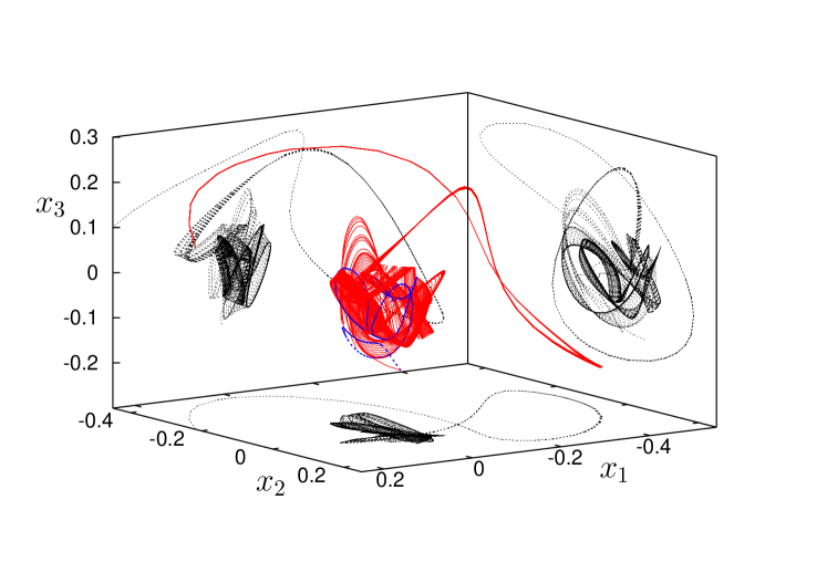
Fig. 1: A piece of the unstable manifold of the periodic orbit at the edge of chaos in a toy model of shear flow. On the axes are the first three Fourier coefficients. The blue curve is the intersection of this piece of manifold with the plane $x_{1}=0$, the rightmost boundary condition. The periodic orbit is located near the equilibrium $x_{1}=1$, $x_{i}=0$ for $i=2,\ldots n$ and is not shown. The computed orbits remain close until they reach the chaotic region, where they flare out exponentially. The corresponding continuation diagram is shown in Fig. 2.

In our model we fix the stream wise to wall normal aspect ratio to $L/H=2.76$ and the span wise to wall normal aspect ration to $W/H=1.88$, corresponding to the minimal flow unit of plane Couette flow [4]. A bifurcation analysis reveals that at $Re=109$ a saddle type and a stable periodic solution are created in a saddle-node bifurcation. The stable orbit loses stability in a torus bifurcation at $Re=256$. The saddle type orbit has a single unstable multiplier for any $Re>109$. This orbit is a small perturbation of the laminar state and can be considered an edge state. In the following, we fix $Re=667$ and compute the unstable manifold of this edge state. A difficulty in this computation is that the unstable multiplier is close to unity. In the example computation it is $\mu_{1}=1.055$.

Fig. 2: The continuation curve corresponding to the piece of manifold shown in Fig. 1. On the horizontal axis the small parameter which fixes the left boundary condition, on the vertical axis the total integration time. In this continuation, there were five shooting intervals and the boundary conditions were given by fixed integration time for the first interval and a Poincaré section $x_{1}=\text{constant}$ for the others.

Fig. 1 shows a piece of the unstable manifold, computed on five shooting intervals with a quadratic local approximation. The right boundary conditions were fixed integration time for the first interval and a Poincaré section for the other intervals. Near the end of the computed orbits there is very strong dependence on initial conditions and the geometry of the manifold is quite complex. The variations in $\epsilon$ are extremely small. Fig. 2 shows the corresponding continuation curve. In this graph, a fold point corresponds to an orbit which is tangent to one of the Poincaré planes of intersection. A detailed account of the geometry of the manifold in the vicinity of such points can be found in Lee et al. [10].

Fig. 3: Convergence results for the computations in the low-order model of shear flow. Left: the residue $\|\mathbf{F}(\mathbf{z})\|$ of the correction step versus the number of Newton-Krylov iterations. The dotted line denotes quadratic convergence. Iterations were stopped when the residue was less than $10^{-8}$. Right: the GMRES residue, normalised by $\|\mathbf{F}(\mathbf{z})\|$, as a function of the Krylov subspace dimension. These results were obtained for the continuation shown in Fig. 2, with five shooting intervals. By proposition 2 the maximal subspace dimension is $14$.

Fig. 3 shows the convergence of the Newton-Krylov iterations. Clearly, the convergence of the Newton iterations is super linear and the number of GMRES iterations satisfies Proposition 2.

In order to compare the multiple shooting algorithm to spectral collocation, we implemented the basic BVP (3) in AUTO [1]. The latest version of this software package allows for thread-parallelisation of the linear solver so that we can compare the performance of the methods for different numbers of processors. Fig. 4 shows the wall time for computing a fixed piece of the continuation curve. For the multiple shooting we used two different strategies. First, we fixed the number of shooting intervals to three. In that case, the computation time decreases approximately by factors of $2/3$ and $1/3$ as we increase the number of CPUs to two and three. After that adding CPUs has no effect. This result is shown with circles. Then, took the number of shooting intervals to be equal to the number of CPUs. In this case, we cannot predict whether the wall time will decrease because the upper bound on the number of GMRES iterations increases linearly with the number of shooting intervals. In practice, we see that the wall time does decrease, albeit slower than linear. This result is shown with squares. AUTO results are shown with triangles. Clearly, wall time taken by AUTO scales nearly linearly over a large range of numbers of CPUs. Nevertheless, the shooting method is faster up to six CPUs.

Fig. 4: Wall time versus the number of CPUs for a representative part of the continuation presented in Fig. 2. The dots have been connected by lines for easy comparison. Triangles represent AUTO results, circles represent shooting on three intervals and squares represent shooting with a variable number of intervals. For precise parameters see text. The scaling of the computation time is linear for the spectral collocation used by AUTO. For shooting on few intervals the wall time is essentially set by the longest integration time.

6.2 Transition in plane Couette flow: many degrees of freedom

Next we compute numerically the unstable manifold of the gentle periodic orbit in a full plane Couette system [7]. This periodic orbit has been obtained at Reynolds number $Re=400$ for the minimal periodic box $(L/H,W/H)=(2.76,1.88)$ [4]. The linear stability analysis of the periodic orbit has shown that there is only one unstable multiplier, implying that the periodic orbit and its stable manifold form the basin boundary between laminar and turbulent attractors [6]. Transitions starting with a disturbance of the laminar flow just beyond a critical amplitude can be described in terms of the unstable manifold of the periodic orbit.

In the computation of the unstable manifold of the gentle periodic orbit we perform direct numerical simulations for the imcompressible Navier–Stokes equation by use of a pseudo-spectral code [5]. In this code the streamwise volume flux and the spanwise mean pressure gradient are set to be zero. The dealiased Fourier expansions are employed in the streamwise and spanwise directions, and the modified Chebyshev-polynomial expansion in the wall-normal direction. Nonlinear terms in the Navier–Stokes equation are computed on $8448$ ($=16\times 33\times 16$ in the streamwise, wall-normal and spanwise direction) grid points. The spatial symmetries observed in a turbulent state of the minimal periodic box are imposed on the periodic orbit [7]. The dealiased symmetric flow field satisfying noslip and impermeable boundary conditions has $2477$ degrees of freedom. Time integration of the equation is performed by using the explicit Adams–Bashforth method for the nonlinear terms and the implicit Crank–Nicholson scheme for the viscous terms.

Fig. 5 shows a piece of the unstable manifold projected on energy input rate, energy dissipation rate and the energy contained in the velocity field after subtracting the average velocity in the stream wise direction. In this computation three shooting intervals were used. The first boundary condition is given by constant integration time and the second by a Poincaré plane of intersection on which the sum of energy input and dissipation rate is constant. The rightmost boundary condition is given by constant arc length. At the edge of the computed piece of manifold, the values of the energy input and dissipation rate are comparable to their time mean value in turbulent flow.

In temporal evolution along the unstable manifold the flow has been found to exhibit the same spatiotemporal behaviour as observed in the transition to turbulence in minimal plane Couette flow. Low-velocity streaks develop with an oscillatory bend in the spanwise direction. During this process the spanwise bend of the streak is enhanced to generate a pair of staggered counter-rotating streamwise vortices in the flanks of the low-velocity streak. The generated streamwise vortices appear to be significant around the intersection $e+\mathcal{E}=6$ which is comparable to the value corresponding to a turbulent state.

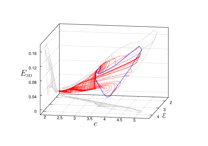
Fig. 5: A piece of the unstable manifolds of the quiescent periodic orbit in plane Couette flow, projected on energy input rate $e$, energy dissipation rate $\mathcal{E}$ and $E_{\rm\scriptstyle 3D}$, the energy contained in the velocity field after subtraction of the average in the stream wise direction. The energy input and dissipation rate have been normalised by their value in laminar flow. This figure can be compared to Fig. 5 of Kawahara and Kida [7], in which a single orbit contained in the unstable manifold is displayed. Although the computed piece of manifold stretches from the near-laminar to the turbulent region in phase space, it looks like a cylinder and the intersection with a Poincaré plane is a simple closed curve. The corresponding continuation diagram is shown in Fig. 6.

Fig. 6 shows the continuation curve corresponding to the piece of manifold of Fig. 5. There are two points where orbits are tangent to the Poincaré plane of intersection. The first and the last point in this diagram correspond to orbits which coincide in the projection of Fig. 5 but in phase space are related by a discrete symmetry composed of a reflection in the span wise direction, combined with a shift in the stream wise direction. This explains why the two orbits differ only by half the period of the quiescent periodic orbit.

Fig. 6: The continuation curve corresponding to the piece of manifold shown in Fig. 5. On the horizontal axis the small parameter which fixes the left boundary condition (3), on the vertical axis the total integration time, normalised by the period of the quiescent periodic orbit. In this continuation, there were three shooting intervals and the boundary conditions were given by fixed integration time, the Poincaré section $e+\mathcal{E}=6.5$ and fixed arc length, respectively. The first and the last point in this continuation correspond to orbits related be a discrete spatial symmetry which leaves the energy invariant.

The convergence results for our computation in Couette flow are shown in Fig. 7. Like for the low-order model, the convergence of the Newton-Krylov iteration is super linear and the dimension of the Krylov subspace satisfies proposition 2.

Fig. 7: Convergence results for the computations in plane Couette flow. Left: the residue $\|\mathbf{F}(\mathbf{z})\|$ of the correction step versus the number of Newton-Krylov iterations. The dotted line denotes quadratic convergence. Iterations were stopped when the residue was less than $10^{-7}$. Right: the GMRES residue, normalised by $\|\mathbf{F}(\mathbf{z})\|$, as a function of the Krylov subspace dimension. These results were obtained for the continuation shown in Fig. 6, with three shooting intervals. By proposition 2 the maximal subspace dimension is $8$.

Finally, we measured the wall time of the computation as a function of the number of CPUs employed, as shown in Fig. 8. In this computation we used five shooting intervals of approximately equal length. With five CPUs active the wall time was one fifth of the wall time with a single CPU to within 5%. The data communicated by MPI comprises only a small number of vectors of length $n$, mounting to less than a megabyte, and the code can easily be run on an ordinary multi core computer.

Fig. 8: Wall time versus the number of CPUs for a representative part of the continuation presented in Fig. 6. The dots have been connected by lines for easy comparison. In each computation five shooting intervals of approximately equal integration time were used. The computation time decreases approximately by factors of $3/5$, $2/5$, $2/5$ and $1/5$ when increasing the number of CPU’s. This behaviour confirms that nearly all time is spent in time stepping the (linearised) Navier-Stokes equations in parallel and the parallelisation is nearly 100% efficient. The dashed line denotes linear scaling.

7 Conclusion

We have presented an efficient and flexible method for computing 2D invariant manifolds of dynamical systems with any number of degrees of freedom. This method is based on the orbit continuation algorithm [8, Sec. 3].The main issue in this computation is the sensitive dependence on initial conditions. Our algorithm deals with this problem by the use of multiple shooting. By we controlling the integration time on each shooting interval we ensure the computation is stable and well-conditioned. By choosing different boundary conditions on each interval we can select different parts of the manifold to compute. The time integrations of the dynamical system and its linearisation on different shooting intervals can be efficiently executed in parallel.

The multiple shooting orbit continuation leads to linear systems of a size which grows as the product of the number of degrees of freedom of the dynamical system and the number of shooting intervals. We have implemented GMRES [12] as a linear solver. Remarkably, Proposition 2 states that the maximal number of GMRES iterations for each Newton update step is linear in the number of shooting intervals but does not depend on the number of degrees of freedom. In practice, this means that if we compute the same piece of manifold several times with an increasing numbers of shooting intervals and parallel processes, there is no guarantee that the computation time will decrease. Normally, however, we will be computing as large a piece as we can with the minimal number of shooting intervals that guarantees convergence. For this approach, our convergence result implies that the computation time will depend only on the time required by the time-stepping and on the condition of the linear system, not its size.

Both example computations in this paper concerned 2D unstable manifolds of periodic solutions to strongly dissipative systems. However, the algorithm has wider applicability. For stable manifolds one can reverse the direction of time, or reverse the role of the left and right boundary conditions. For (un)stable manifolds of equilibria, the left boundary condition can be formulated in terms of the two (un)stable eigenvectors. Moreover, the result on convergence of GMRES iterations does not rely on any assumptions on the properties of the linearised system. Thus, we expect the Newton-Krylov orbit continuation algorithm to be equally suitable for the computation of manifolds in general high-dimensional dynamical systems such as networks of chaotic oscillators.

References

- [1] E. J. Doedel, A. R. Champneys, T. F. Fairgrieve, Y. A. Kuznetsov, B. Sandstede, and X. Wang, AUTO97: Continuation and bifurcation software for ordinary differential equations, 1997. Concordia University, Montreal, Québec, Canada.
- [2] B. Eckhardt, H. Faisst, A. Schmiegel, and T. M. Schneider, Dynamical systems and the transition to turbulence in linearly stable shear flows, Philos. Trans. R. Soc. Lond. Ser. A Math. Phys. Eng. Sci., 366 (2008), pp. 1297–1315.
- [3] W. S. Edwards, L. S. Tuckerman, R. A. Friesner, and D. C. Sorensen, Krylov methods for the incompressible Navier-Stokes equation, J. Comp. Phys., 110 (1994), pp. 82–102.
- [4] J. M. Hamilton, J. Kim, and F. Waleffe, Regeneration mechanisms of near-wall turbulence structures, J. Fluid Mech., 287 (1995), pp. 317–348.
- [5] T. Itano and S. Toh, The dynamics of bursting process in wall turbulence, J. Phys. Soc. Japan, 70 (2001), pp. 703–716.
- [6] G. Kawahara, Laminarization of minimal plane couette flow: Going beyond the basin of attraction of turbulence, Phys. Fluids, 17 (2005), p. 041702.
- [7] G. Kawahara and K. Kida, Periodic motion embedded in plane couette turbulence: regeneration cycle and burst, J. Fluid. Mech., 449 (2001), pp. 291–300.
- [8] B. Krauskopf and H. M. Osinga, Computing invariant manifolds via the continuation of orbit segments, in Numerical Continuation Methods for Dynamical Systems, B. Krauskopf, H. M. Osinga, and J. Galan-Vioque, eds., Springer, 2007, pp. 555–666.
- [9] B. Krauskopf, H. M. Osinga, E. J. Doedel, M. E. Henderson, J. Guckenheimer, M. Dellnitz, and O. Junge, A survey of methods for computing (un)stable manifolds of vector fields, Int. J. Bifurc. Chaos, 15 (2005), pp. 763–791.
- [10] M. C. Lee, P. J. Collins, B. Krauskopf, and H. M. Osinga, Tangency bifurcations of global poincaré maps, SIAM J. Appl. Dyn. Syst., 7 (2008), pp. 712–754.
- [11] J. Moehlis, H. Faisst, and B. Eckhardt, Periodic orbits and chaotic sets in a low-dimensional model for shear flows, SIAM J. Appl. Dynam. Syst., 4 (2005), p. 352.
- [12] Y. Saad and M. H. Schultz, GMRES: A generalized minimal residual algorithm for solving nonsymmetric linear systems, SIAM J. Sci and Stat. Comput, 7 (1986), p. 856.
- [13] J. Sánchez and M. Net, On the multiple shooting continuation of periodic orbits by Newton-Krylov methods, Int. J. Bifurc. Chaos, 20 (2010). In press.
- [14] J. Sánchez, M. Net, B. García-Archilla, and C. Simó, Newton-krylov continuation of periodic orbits for Navier-Stokes flows, J. Comp. Phys., 201 (2004), pp. 13–33.
- [15] J. Sánchez, M. B. Net, and C. Simó, Computation of invariant tori by Newton-Krylov methods in large-scale dissipative systems, Phys. D, 239 (2010), pp. 123–133.
- [16] F. Waleffe, On a self-sustaining process in shear flows, Phys. Fluids, 9 (1997), pp. 883–900.