Optical Colors of Intracluster Light in the Virgo Cluster Core

Abstract

We continue our deep optical imaging survey of the Virgo cluster using the CWRU Burrell Schmidt telescope by presenting $B$-band surface photometry of the core of the Virgo cluster in order to study the cluster’s intracluster light (ICL). We find ICL features down to $\mu_{B}$$\approx 29$ mag arcsec^-2, confirming the results of Mihos et al. (2005), who saw a vast web of low-surface brightness streams, arcs, plumes, and diffuse light in the Virgo cluster core using $V$-band imaging. By combining these two data sets, we are able to measure the optical colors of many of the cluster’s low-surface brightness features. While much of our imaging area is contaminated by galactic cirrus, the cluster core near the cD galaxy, M87, is unobscured. We trace the color profile of M87 out to over 2000″, and find a blueing trend with radius, continuing out to the largest radii. Moreover, we have measured the colors of several ICL features which extend beyond M87’s outermost reaches and find that they have similar colors to the M87’s halo itself, $B-V$$\approx 0.8$. The common colors of these features suggest that the extended outer envelopes of cD galaxies, such as M87, may be formed from similar streams, created by tidal interactions within the cluster, that have since dissolved into a smooth background in the cluster potential.

1. Introduction

Massive galaxy clusters are known to contain a population of stars which reside outside of any of the cluster’s galaxies, often referred to as intracluster light or ICL. ICL features typically have extremely faint surface brightnesses of $<1\%$ of the brightness of the night sky, making their study extremely difficult. While the first indications of the existence of ICL came from observations by Zwicky (1951), only with the advent of modern CCD technologies have detailed studies of these stars been made possible (e.g., Uson et al. 1991; Vílchez-Gómez et al. 1994; Bernstein et al. 1995; Gregg & West 1998; Trentham & Mobasher 1998).

The most straightforward method of detecting the ICL is through deep broadband imaging at optical wavelengths (e.g., Uson et al. 1991; Vílchez-Gómez et al. 1994; Trentham & Mobasher 1998; Feldmeier et al. 2002, 2004a; Mihos et al. 2005, hereafter referred to as M05; Gonzalez et al. 2005; Krick & Bernstein 2007). With such imaging, we can not only measure the luminosity of ICL the component, but we can study its spatial distribution and detect individual ICL features, such as streams, arcs, and plumes (e.g., Gregg & West 1998; Trentham & Mobasher 1998; Calcáneo-Roldán et al. 2000; White et al. 2003; M05; Krick et al. 2006; Yagi et al. 2007) as well as any large-scale diffuse components (e.g., Gonzalez et al. 2000; Feldmeier et al. 2002, 2004a; Adami et al. 2005; Zibetti et al. 2005; Patel et al. 2006; Krick & Bernstein 2007; Pierini et al. 2008; Da Rocha et al. 2008). ICL has also been detected using discrete stellar tracers (e.g., Ferguson et al. 1998; Feldmeier et al. 1998; Durrell et al. 2002; Gal-Yam et al. 2003; Arnaboldi et al. 2004; Feldmeier et al. 2004b; Gerhard et al. 2005; Aguerri et al. 2005; Neill et al. 2005; Maoz et al. 2005; Williams et al. 2007; Castro-Rodriguéz et al. 2009; McGee & Balogh 2010), although these methods often lack the ability to detect individual ICL features.

Intracluster light is thought to form primarily by the tidal stripping of stars as galaxies interact and merge during the hierarchical accretion history of the cluster, causing the fraction of the cluster’s luminosity found in the ICL to increase as it evolves (e.g., Napolitano et al. 2003; Murante et al. 2004; Willman et al. 2004; Rudick et al. 2006; Monaco et al. 2006; Conroy et al. 2007; Murante et al. 2007; Purcell et al. 2007; Yan et al. 2009; Baria et al. 2009). Numerous mechanisms for generating the ICL have been proposed, including the infall of groups into the cluster potential (Willman et al. 2004; Rudick et al. 2006), high speed encounters within the cluster (Moore et al. 1996; Gnedin 2003), and galactic mergers during the buildup of the massive central galaxy (Murante et al. 2007; Conroy et al. 2007). All of these processes are likely to be occurring simultaneously and each will create distinct observable signatures (Rudick et al. 2009). Thus, the formation of ICL is intimately linked to the dynamical history of the cluster, and the observable features of the ICL should contain a great deal of information about the evolutionary processes which have shaped both the cluster and its constituent galaxies.

While ICL is generally thought of as stellar material found outside of any individual galaxy, in practice galaxies have no well-defined edge (Abadi et al. 2006). Thus, the distinction between the ICL and the outer luminosity profiles of cluster galaxies, which display similar surface brightnesses in broadband imaging, is difficult and somewhat arbitrary (M05). In fact, simulations of the formation of clusters’ most massive elliptical galaxies have shown that their extended stellar profiles form through similar merger and tidal stripping mechanisms as the more diffuse ICL (Dubinski et al. 1998; Monaco et al. 2006; Conroy et al. 2007; Murante et al. 2007; Ruszkowski & Springel 2009). We therefore prefer to use intracluster light as a qualitative description of cluster luminosity at low surface brightness, which may refer to individual tidal streams, extreme galactic outskirts, or any large-scale diffuse luminosity component, and which are all likely products of tidal stripping and disruption of galaxies during the dynamical evolution of the cluster.

In addition to the quantity and morphology of the ICL, knowledge of the underlying stellar populations also provides a vital tool for understanding its formation. Giant elliptical galaxies are known to display radial color gradients, whereby the color index decreases, or becomes bluer, with increasing radius (e.g., Pettit 1954; de Vaucouleurs 1961; Carter & Dixon 1978; Strom & Strom 1978; Davis et al. 1985; Vader et al. 1988; Goudfrooij et al. 1994; Bernardi et al. 2003; Cantiello et al. 2005; Liu et al. 2005), primarily due to gradients in the stellar metallicities (e.g., Spinrad et al. 1972; Strom et al. 1976; Baum et al. 1986; Carollo et al. 1993; Tamura et al. 2000; Sánchez-Blázquez et al. 2007; Rawle et al. 2010). Just as the strength of these gradients is an important clue in reconstructing the formation history of elliptical galaxies, the ages and metallicities of the intracluster stars will be highly dependent on the progenitor galaxies from which they were stripped. The results of Sommer-Larsen et al. (2005) show that the metallicity of the ICL is expected to be on average similar to that of the outer envelope of the cD galaxy, while Purcell et al. (2008) show that individual ICL streams formed by recent interactions should be more metal rich than the surrounding diffuse component. Murante et al. (2004) have shown that the diffuse ICL stellar population is expected to be older, on average, than the galactic stars.

Observationally, it is very difficult to break the age-metallicity degeneracy and make precise determinations of either quantity. Although Williams et al. (2007) used HST ACS imaging of red giant branch stars in the Virgo cluster to do so, such observations are only possible in the most nearby systems and span very small fields of view. Their work found that the ICL is composed of stars with a wide variety of ages and metallicities, but that the dominant component is old ($\lower 2.15277pt\hbox{$\;\buildrel>\over{\sim}\;$}10$ Gyr) and moderately metal poor ([M/H]$\lower 2.15277pt\hbox{$\;\buildrel<\over{\sim}\;$}-1.0$). A more common technique is to instead use broadband optical colors in order to compare the ICL stellar populations to those of galactic stars. Most studies have found results consistent with Williams et al. (2007), where the average ICL color is similar to that of the outer halo of the cluster’s brightest galaxy (e.g., Zibetti et al. 2005; Pierini et al. 2008; da Rocha et al. 2008), which due to radial color gradients is bluer than the galaxy’s interior regions. However, a number of clusters have been observed to have an ICL component with significantly redder colors, more similar to the brightest galaxy’s interior (Krick & Bernstein 2007; da Rocha & Mendes de Oliveira 2005; Gonzalez et al. 2000).

As part of our ongoing deep imaging survey of the Virgo cluster using Case Western Reserve University’s Burrell Schmidt telescope, this paper presents deep imaging of the Virgo cluster core in the $B$-band. By combining this data with the $V$-band results previously published in M05, we are able to measure the optical colors of Virgo’s intracluster light. A detailed description of our data acquisition and reduction techniques is given in Section 2. Our $B$-band image is presented in Section 3, while Section 4 combines the two images in order to measure the colors of ICL features. Section 5 includes a summary of our results and a discussion of our interpretations. Finally, detailed error models for our photometric measurements can be found in the Appendix.

2. Observations and Data Reduction

2.1. Observations

Our imaging data was collected on dark photometric nights on three separate observing runs spanning January through March of 2009, using the 0.6m CWRU Burrell Schmidt Telescope located at Kitt Peak National Observatory. The Burrell Schmidt’s closed-tube optical design makes it ideal for wide-field, deep optical imaging. Using a 4096$\times$4096 pixel CCD read out of 4 amplifiers simultaneously, the 1.45″ pixel scale results in a field of view which exceeds 2.5 square degrees. Further details of the CWRU Burrell Schmidt’s optical system can be found in Nassau (1945) and Slater et al. (2009).

The observations described in M05 were made using the Washington $M$ filter, converted to Johnson $V$ magnitudes. To measure the colors of the ICL features seen in those observations, we could have selected to re-observe the area in either a bluer or redder filter. However, at redder wavelengths, emission lines in the atmosphere cause the night sky to vary considerably in brightness on timescales of minutes (Feldmeier et al. 2002 and references therein), which would severely hamper our ability to accurately flat field and sky-subtract our data. While both our targets and the sky are fainter in the blue, requiring longer observing times, the stability of the night sky emission made the selection of a blue filter the natural choice.

Because the Washington $M$ filter is somewhat shifted blue-ward of the $V$ filter, and to ensure adequate wavelength separation between our two filters, for these observations we used a custom-designed filter, referred to as $B^{\prime}$, with an effective wavelength $\approx 200\AA$ shorter than the standard Johnson $B$ filter. All surface brightness measurements, however, have been transformed to the Johnson $B$ system.

Our observational and data reduction techniques are based on those described in Morrison et al. (1997), Feldmeier et al. (2002), M05, and Slater et al. (2009). Because of the diffuse, extremely faint nature of the ICL features we are measuring ($0.1-1\%$ of the brightness of the night sky), generating a flat-field which exceeds this precision over the entire field of view is of critical importance. We therefore constructed a night-sky flat from pointings of pre-selected sky fields, chosen to be offset from our target field by $\approx 0.25-1$ hours in right ascension and less than $\approx 4$° in declination, while containing relatively low stellar density and no particularly bright stars. Our observing schedule was roughly evenly divided between imaging our target and the offset sky fields. A typical observation cycle consisted of 2 sky images offset west, 4 images on the target field, and 2 more sky images offset east, repeated throughout the night. By minimizing the motion of the telescope during the cycle, this pattern reduced any hysteresis effects caused by flexure of the optical system and ensured that the sky frames were taken as close in time and position as possible to the target images, under similar atmospheric and telescope conditions. When imaging the target field, individual pointings were intentionally offset in a dither pattern from the field center by as much as 0.75°, or half the size of the field of view, in order to reduce systematic effects which may result from consistently imaging objects with the same area of the CCD. All sky and target field images were 1200 second integrations, yielding a sky brightness of $\approx 750$ ADU.

2.1.1 Sources of Diffuse Light

Although the scientific aim of our survey is to image the intracluster light in the Virgo galaxy cluster, we are, of course, sensitive to all sources of low-surface brightness diffuse light. In practice, we detect two major sources of diffuse light: ICL in the Virgo cluster and light scattered by galactic cirrus within our own Galaxy (e.g., Sandage 1978; Guhathakurta & Tyson 1989; Witt et al. 2008). For the purposes of image processing and data reduction, all diffuse light sources are equivalent and we make no distinction between luminosity from galactic or extra-galactic sources. For scientific analyses, however, the source of the diffuse light can be critical to the interpretation of our results, and the impact of galactic cirrus is discussed in Section 3.2.

2.2. Image Pre-Processing, Photometric Solutions, and Data Quality Cuts

Our image processing procedure began by subtracting a nightly bias frame, applying a CCD overscan region correction, and removing amplifier crosstalk from all images, each in the usual manner (hereafter, these images are referred to as pre-processed). The images were then flattened using a preliminary flat field generated by a simple median combination of all of our sky frames scaled by their mode, using the imcombine task from the IRAF software package . Although the input sky images were not put through the rigorous screening and processing required to create a final flat field (see Section 2.3), pixel values in this preliminary flat field, created from 111 individual images, differed from the final version by typically $<0.5\%$. An astrometric solution for each image was calculated using the Astrometry.net software package (Lang et al. 2010), and an airmass correction was applied.

Photometric zeropoints for all images were then calculated by comparing the stellar fluxes, as measured using IRAF’s daophot routines, to those found in the Sloan Digital Sky Survey DR7 catalog (Abazajian et al. 2009), transformed to Johnson $B$ magnitudes (Ivezic et al. 2007). From this analysis, we calculated a $B-V$ color term of 0.05 mag to transform our data to the Johnson $B$ system. For each night of observations we calculated and subtracted a nightly zeropoint, taken to be the mean of all zeropoints from that night. After subtracting this nightly zeropoint, all images were set to a common photometric zeropoint. For a typical $B-V$ color of 1.0, 1 ADU corresponds to 29.6 mag arcsec^-2.

A data quality cut was made by excluding images from nights found to have highly variable photometric zeropoints, indicative of light cloud cover or other non-photometric conditions. We calculated the mean and scatter in zeropoint for all images and excluded any data from nights on which the photometric zeropoint varied by $>2\sigma$ from the mean, or approximately 0.02 mag. This quantitative measure of photometric atmospheric conditions agreed remarkably well with observer notes from the nightly observation logs.

2.3. Flat Field

Our flat field was constructed using the offset sky images described in Section 2.1. The primary motivation for using this sky-flat method is that we expect the detector response to be wavelength-dependent. By using the night sky as our uniform illumination source, we ensure that the flat field is measured at the same effective wavelength as our target sources. Because the diffuse light sources we are measuring are $<1\%$ of the brightness of the night sky, we are dominated by sky photons even in our target frames. Moreover, we expect the ICL itself to be similar in color to the night sky (Taylor et al. 2004; Sommer-Larsen et al. 2005), further motivating the use of the night sky as our uniform illumination source.

The first step in creating the final flat field was to use IRAF’s objmask task to find and mask all objects in each image, including stars, galaxies, satellite trails, and any other bright features. Because our goal is to measure a uniform illumination pattern as well as possible, we used an aggressive masking technique whereby we ran objmask twice, first on the original image and again after masking out any objects found in the first run. Once the object masks were applied, we median-binned the images in 128$\times$128 pixel groups, and visually inspected each frame to check the image quality and search for and mask any remaining diffuse, non-sky features. All images had some features which were masked by hand, including the extended wings of bright stars, internal reflections, and flares from stars near the edge of the field of view. A number of images were discarded due to the presence of strong galactic cirrus, a particularly bright star on the image, or other features which created a large-scale illumination pattern. After this quality cut we were left with 84 night sky images with which to create the final flat field.

Due to variations in the atmospheric conditions of each observation, such as airglow, transparency, airmass, etc., the mean flux level of the night sky varies from image to image, typically in the range of 650-850 ADU, or $\mu_{B}$=22.6-22.3 mag arcsec^-2. However these effects not only cause the mean sky level to vary, they are also the cause of an illumination gradient over the field of view of each image, typically in the range of 5-10 ADU, or $\approx 1\%$ of the sky flux across the frame. In order to account for these atmospheric effects and create a flat field representing a uniform illumination pattern, we employed an iterative process to combine the night sky images into our final flat field, following Morrison et al. (1997). We began by flattening the pre-processed sky images using the preliminary flat field and then applied both the object and hand masks. The sky gradients were removed by binning and fitting a plane to each image, and then dividing the pre-processed images by this normalized sky plane. We then re-applied the object and hand masks, and median combined all the frames to make the new flat field. This process was then repeated, except that the pre-processed data were flattened with the new flat field. After only a few iterations, the resulting flat field converged. As a further check of the robustness of our combination technique, we made several flat field images from a random selection of half of our sky images; pixels varied in these half-split flats with a standard deviation of $\approx 0.5\%$, consistent with the errors expected from photon statistics (see the Appendix for a discussion of photon statistics and other sources of photometric error in the final images). All pixels which were either under-illuminated by over 50% from the mean or which varied strongly in the half-split flats — these pixels were typically associated with small dust spots or very near the edge of the CCD, and represent $<0.5\%$ of the pixels — were masked in the target frames.

During our processing of the sky images into a flat field, we noticed a systematic difference between images taken during the third observing run and those taken during the first two runs. Frames from the third run showed a characteristic radial dimming pattern whereby pixels farthest away from the image center were under-illuminated by $\approx 2\%$. We believe this effect to be the result of a thermal gradient, whereby the center of the CCD was cooled less efficiently, and was therefore warmer, than the outskirts during this run. However, we find no indication that the flat field characteristics varied temporally within the third run. Fortunately, because the weather during the final run was significantly better than in the preceding runs, a disproportionate fraction of our data was taken during run three, giving us an ample number of exposures with which to construct a separate flat field. We thus generated two final flat fields, one for the first two runs using 47 sky images, and another for the third run from 37 sky frames. Our target images were then flattened by dividing by the final flat field corresponding to the run in which they were taken. In Section 2.6 we show that the final mosaic image is not affected by any run-specific effects.

2.4. Star Subtraction

Figure 1.— Solid line: the extended wings of our model stellar profile for a $m_{B}=0$ star. Dotted line: Our model PSF, excluding reflections from the dewar window surfaces. Dashed and dot-dash lines: the contributions to the stellar profile from the inner and outer dewar window surfaces, respectively, for a star with axisymmetric reflections. Unlike the data used in Slater et al. (2009) taken using the Washington-$M$ filter, we see no measurable reflections from the $B^{\prime}$ filter surfaces.

A key element of our data processing technique was to remove scattered light from stellar sources in our target images using the methods developed in Slater et al. (2009). As Slater et al. (2009) showed, the combination of extended stellar profiles plus scattered light from internal reflections within the optical system can cause a spurious diffuse signal which would contaminate the very faint ICL signal we are trying to measure. Moreover, the internal reflections are not axisymmetric about the star, and are dependent on the star’s position within the field of view. Thus, in addition to taking both our sky and target images, during our observing runs we also took numerous images of bright stars, varying the position of the star within the field of view, in order to trace the stellar PSF and internal reflections. We acquired 13 900 s exposures of $\beta$ Gem ($m_{B}=2.14$), five 900 s exposures of $\alpha$ Boo ($m_{B}=1.19$), and four 1200 s exposures of $\alpha$ Gem ($m_{B}=2.00$), as well as several short (1-15 s) exposures of these stars. Using these images, we determined the amplitude and position of reflections off the optical surfaces and measured the stellar PSF to a radius of over 0.5°. We show the extended wings of our model stellar profile in Figure 1.

In order to subtract the stellar contribution from our target images, for each image we created a map of the stellar light by reconstructing the profile of each star in the image, including the position-dependent internal reflections. Stellar brightnesses were measured from short (1-60 s) exposures of our target field taken during the observing runs and the profile of each star was scaled to match its flux. We mapped the profile of each star out to the radius at which it fell below 0.3 ADU and subtracted these profiles from the individual target frames.

2.5. Sky Subtraction

In exactly the same manner as the sky frames discussed in Section 2.3, each target image contains a sky flux level which varies between images, and spatially across each image. However, whereas fitting a plane to the sky signal was straightforward for the sky images because the vast majority of their pixels were of empty sky, the target field is permeated by large galaxies and extended diffuse light, meaning that there is essentially no true sky to measure. Because the sky and diffuse light signals vary by similar amplitudes over similar scales, it is extraordinarily difficult to disentangle the two and remove only the sky signal.

We began the sky subtraction process by running two rounds of objmask, masking image artifacts such as star flares and reflections by hand, and spatially binning the image, in the same manner as we processed the sky images in Section 2.3. M05 attempted to use an iterative process to minimize the frame-to-frame scatter in the intensity of pixels at the same location after sky subtraction. However, subsequent testing has revealed that our implementation of this technique achieved results not significantly better than simply fitting a single sky plane to each target image (see the Appendix for details). We have therefore utilized this simpler technique, and the sky signal was removed by fitting a plane to each target frame in the same manner as for the sky images.

This inability to accurately fit the night-sky signal results in our largest source of systematic uncertainty across large scales, creating an uncertainty of 1-2 ADU across the majority of the image, discussed in detail in the Appendix. Additionally, because the entire target region is permeated with diffuse light, determining the sky zero level, or the flux level of “pure” sky, was also extremely difficult. We selected several regions of the image which looked by eye to be the darkest, or least diffuse light-contaminated, and defined the sky level to be the mean pixel value in these regions. We emphasize that this is likely to be somewhat brighter than the true sky level as these regions probably contain some diffuse light, and that this could lead to a systematic over-subtraction of any large-scale diffuse light component. Fundamentally, these are issues which are inherent to any surface photometry measurements in which the objects fill the field of view, making a precise determination of the sky flux extremely difficult.

2.6. Creating The Final Mosaic

After sky subtraction, the final processing step was to simply apply a photometric airmass correction to each target image. The fully-processed frames were then registered and all 102 images were median combined into a mosaic using imcombine, using a 3-$\sigma$ rejection to remove outlying pixel values. All regions of the mosaic which did not contain a minimum of five exposures were masked. After creating the initial mosaic, a final sky plane was fit and removed, in the same manner as described in Section 2.5; this plane had an amplitude of $\approx 0.5$ ADU across the width of the mosaic.

As a test of the robustness of our sky subtraction and image mosaicking procedures, we created numerous mosaics from subsets of input images and compared these to the final mosaic. The input frames were divided into subsets based on various parameters, including the run, airmass, hour angle, right ascension, declination, sky brightness, and local time of the observation. Only when we split the input images by right ascension (i.e. the position of the image within the mosaic), did we see any significant large-scale variations from the final mosaic, and these variations were of only $\approx 0.5$ ADU. This effect is most likely caused by specific diffuse light features which were present in certain areas of the mosaic which would have systematically influenced the fit of the sky plane.

3. $B$-band Mosaic Image

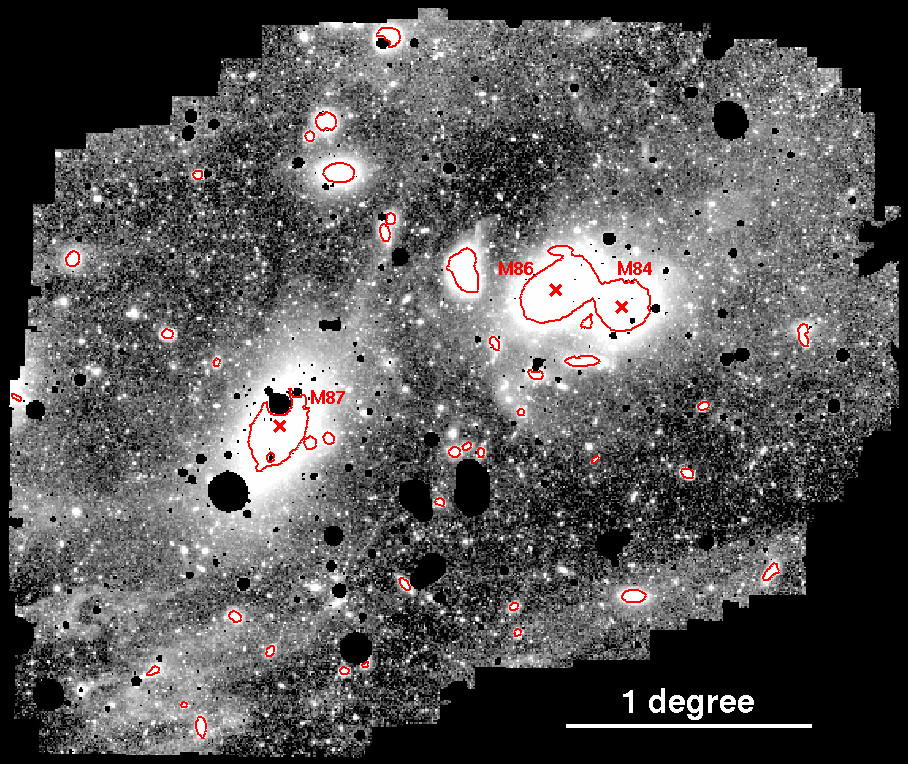
Figure 2.— $B$-band mosaic image of the Virgo cluster core (north is up, east is left). The low-surface brightness features seen in this image are qualitatively extremely similar to those seen in the $V$-band imaging of M05 (see Figure 1). All regions containing fewer than five exposures have been masked. Also, stars have been masked out to the radius where their subtracted profile falls below 5 ADU. The pixels have been binned in 16$\times$16 groups (23.2″$\times$23.2″) in order to increase the signal-to-noise and display faint features. The centers of the three giant elliptical galaxies in the field, M87, M86, and M84 have been marked with X’s, and the red lines indicate the $\mu_{B}$=25 mag arcsec^-2 isophotes for a selection of the cluster’s most luminous galaxies.

3.1. ICL Features

Figure 2 shows our final mosaic, binned in 16$\times$16 pixel groups (23.2″$\times$23.2″), with bright stars masked. Qualitatively, the $B$-band image of the Virgo cluster core shown in Figure 2 appears almost exactly like the $V$-band image from M05, albeit with a significantly larger mosaic area due to the increased CCD size. In fact, every feature identified in M05 appears in this image, including the distorted outer halo of M87, the two tidal streams extending northwest of M87, the doglegged plume to the north of NGC 4435/4438, the common envelope around NGC 4413/IC 3363/IC 3349, and many other features as well (see M05 Figure 3 for a schematic finding chart of ICL features in this field). The identification of these features in a second imaging survey, using a different filter and with a modified instrumental set-up confirms the robustness of our imaging techniques and the veracity of these extremely faint structures.

3.2. Galactic Cirrus

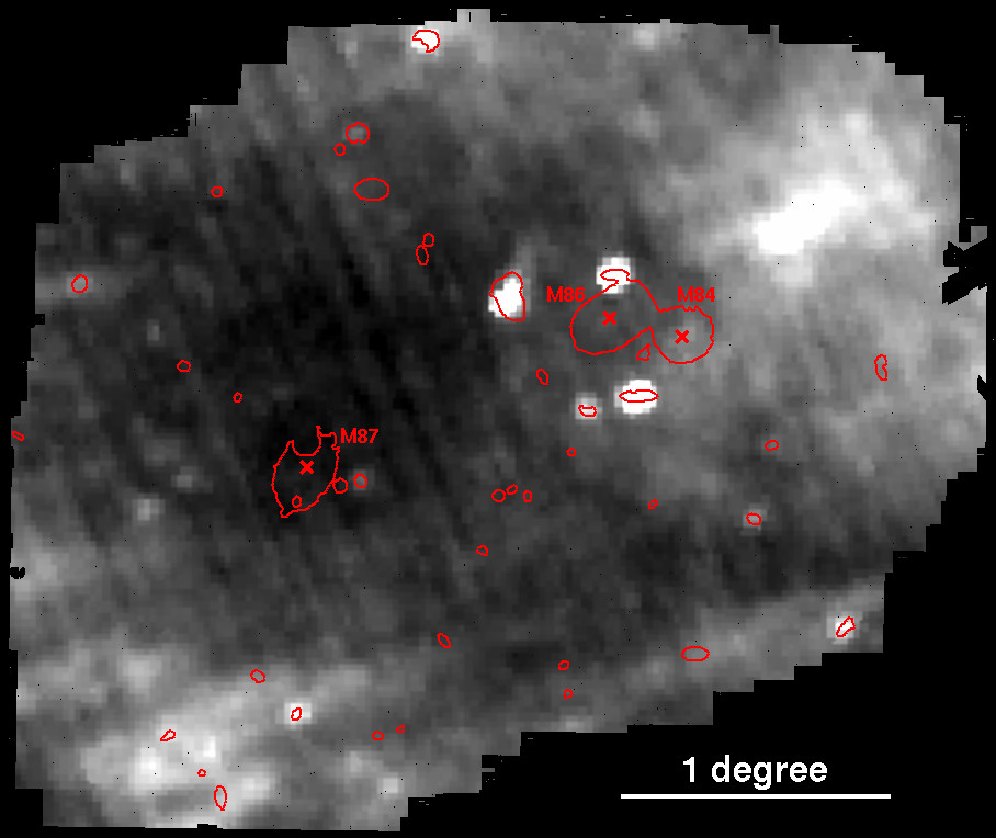
Figure 3.— IRAS 100$\mu$m map of the Virgo cluster core from Schlegel et al. (1998), on the same pixel scale as Figure 2 with the $B$-band exposure mask applied. As in Figure 2, the centers of the three giant elliptical galaxies in the field, M87, M86, and M84 have been marked with X’s, and the red lines indicate the $\mu_{B}$=25 mag arcsec^-2 isophotes for a selection of the cluster’s most luminous galaxies. Diffuse features are indicative of galactic cirrus, including the large knot in the northwest, the bright emission in the southeastern corner, and the long streak running nearly parallel to the southwestern border of the mosaic. We find corresponding optical emission for all of these features, and must exclude these regions from our analysis of the ICL. Fortuitously, the region to the northwest of M87 containing the three prominent tidal features discussed in Section 4.2.1 contains very little galactic cirrus.

In addition to ICL in the Virgo cluster, another significant large-scale, low-surface brightness astrophysical feature seen in this image is galactic cirrus. Galactic cirrus is composed of dust clouds within the Galaxy which reflect galactic starlight (e.g., Sandage 1976; Witt et al. 2008). These cold dust clouds are most readily detected through their thermal emission in the far-infrared. Figure 3 shows the Schlegel et al. (1998) IRAS 100$\mu$m image of our mosaic field. The galactic cirrus features are most obviously seen in the southeast, northwest, and southwest corners of our $B$-band mosaic and match extremely well to far-infrared emission. Fortuitously, the core of the Virgo cluster, which contains the majority of the ICL features we wish to measure, is relatively unaffected by galactic cirrus. However, the cluster core is surrounded by a ring of cirrus which obscures any ICL which may lie behind it. These galactic cirrus features were not as readily apparent in the $V$-band image of M05 since most of the cirrus lies outside of the smaller field of view of that data set. Because these cirrus features have no consistent optical color (Guhathakurta & Tyson 1989; Witt et al. 2008) and vary in intensity on very small scales, we do not attempt to model and subtract them from the data and must simply ignore any areas affected by these features for the purposes of measuring ICL.

4. ICL $B-V$ Colors

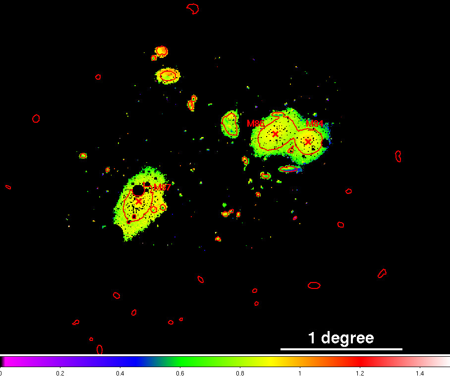
Figure 4.— $B-V$ color map of the Virgo core in the regions of overlap between our two mosaic images, on the same pixel scale as Figure 2. As in Figure 2, the centers of the three giant elliptical galaxies in the field, M87, M86, and M84, have been marked with X’s, and the red lines indicate the $\mu_{B}$=25 mag arcsec^-2 isophotes for a selection of the cluster’s most luminous galaxies. Bright stars and all pixels with $\mu_{V}$$>27.0$ mag arcsec^-2 or $\mu_{B}$$>27.5$ mag arcsec^-2 have been masked. As discussed in detail in the text, features at lower surface brightness are subject to large systematic errors which cause measurements of their colors to be unreliable over large scales. The colors in the central regions of galaxies have an asymmetric profile due to a small ($\lower 2.15277pt\hbox{$\;\buildrel<\over{\sim}\;$}1$″) coordinate registration offset between the $B$ and $V$ images.

By combining our $V$-band imaging data from M05 with our current $B$-band dataset, we can measure the $B-V$ colors of the diffuse light in the Virgo cluster core. However, because we have estimated the sky emission differently for our $B$-band data than for the $V$-band data presented in M05 (described in Section 2.5), for consistency we have re-reduced that data using the new sky subtraction method. This has only a very minor effect on the resulting mosaic and all the features described in that work remain qualitatively similar; a more quantitative discussion of the differences between these two sky subtraction techniques can be found in the Appendix.

A major challenge in generating a large-scale color map of the cluster is setting the proper sky flux level for both images. Not only is the absolute image sky level difficult to determine precisely (see Section 2.5), but within each image we also have large-scale sky level uncertainties which we estimate to be of order 1-2 ADU (see the Appendix). Because the features we are measuring have very low flux levels, even small errors in the sky levels can translate into substantial differences in the final colors. For example, at $\mu_{V}$=28 mag arcsec^-2, a sky level offset of just 1 ADU becomes a 0.4 mag. uncertainty in the $B-V$ color. At higher flux levels this effect is significantly reduced as the sky level uncertainty becomes a very small fraction of the total flux; at $\mu_{V}$=26 mag arcsec^-2, a 1 ADU zero level offset translates to only a 0.07 mag. uncertainty in the $B-V$ color. Figure 4 shows our $B-V$ color map in the region of overlap between the two mosaic images, which is limited primarily by the $V$-band areal coverage. The image is shown on the same pixel scale as Figure 2, with all pixels at surface brightness $\mu_{V}$$>27.0$ mag arcsec^-2 or $\mu_{B}$$>27.5$ mag arcsec^-2 masked.

Each of the three giant elliptical galaxies — M87, M86, and M84 — shows a very red central core with a distinct radial gradient trending bluer in the outskirts, in excellent agreement with previous studies (e.g., Carter & Dixon 1978; Davis et al. 1985; Goudfrooij et al. 1994; Bernardi et al. 2003; Liu et al. 2005). In this image, however, each of these and several other galaxies shows an azimuthally varying color gradient in the innermost regions. This is an instrumental effect caused by very small (sub-arcsecond) offsets in the coordinate registrations of the $B$ and $V$ images, coupled with the very steep luminosity gradients present in the galactic centers. The two data sets were taken several years apart, with different CCDs, on a telescope which underwent substantial modification to its optical system in the intervening years. The resulting high-order distortions make it exceedingly difficult to register the entire field of view to the sub-arcsecond precision needed to precisely measure the rapidly varying inner regions of galaxies, and our survey was never designed to accomplish this. Instead, our analyses are concentrated on the diffuse outer regions of galaxies which are not effected by these minute registration offsets, due to the large angular sizes of these features.

At very low surface brightnesses the sky level uncertainties discussed above make any determination of the color from such a large-scale map highly problematic. Indications of these effects can indeed be seen in the upper left corner of this image, particularly in the galaxies NGC 4473 and 4477, which appear particularly red. Due to the specific geometry of the images which compose our mosaic, this is the region in which our sky level uncertainties are largest. We believe our sky level uncertainties in this area to be up to 3-4 ADU, which could easily lead to uncertainties of several tenths of a magnitude in $B-V$ color, even at the relatively high surface brightnesses shown. At surface brightnesses fainter than the $\mu_{V}$$>27.0$ mag arcsec^-2, $\mu_{B}$$>27.5$ mag arcsec^-2 limits shown in Figure 4, these issues become even more pronounced, making such a large scale map an unreliable source for determining the color of ICL features.

In order to better measure the colors of interesting ICL features, we have developed two methods with which to measure colors and estimate the photometric errors, depending on the features’ angular scales. For large, degree-scale objects, such as the extended stellar envelope of M87, the dominant uncertainty comes from our sky level gradients, which we can estimate and include in our error model. Over the smaller, $\lower 2.15277pt\hbox{$\;\buildrel<\over{\sim}\;$}10$′ scales of individual tidal streams, other systematic effects dominate, and we have developed a local background subtraction technique which allows us to more robustly estimate and reduce systematic uncertainties. The sections below provide examples of these techniques and measure the colors of many of the image’s most interesting low-surface brightness features, while the error budgets are described in the Appendix.

4.1. Extended Stellar Envelope of M87

Our analysis of the luminosities, shapes, other $V$-band photometric properties of M87 and other Virgo giant ellipticals can be found in Janowiecki et al. (2010). Here, we focus solely on the $B-V$ color properties of M87. Because the outer regions of the other two giant elliptical galaxies in the field, M84 and M86, overlap one another in projection, we have not attempted similar analyses for these galaxies.

Figure 5.— Color profile of M87’s extended stellar halo. Squares are the color using all pixels in the bin, with $\pm 1$ ADU error bars. Circles show the azimuthal color variance by measuring the color in eight equal angle slices at each radius (see text for details), offset slightly right for clarity. The dotted line is a fit to the color profile inside of 1000″, and has a slope of $\Delta(B-V)/\Delta(\log(SMA))=-0.11$.

We have measured M87’s color in elliptical annular bins, defined by the galaxy’s $V$-band isophotes as measured by Janowiecki et al. (2010). As in that work, before measuring the galaxy luminosity, small-scale sources were masked using objmask. To effectively detect these sources, we subtracted a ring-median smoothed image from the original, thus removing the large-scale galaxy luminosity distribution and leaving only the small-scale sources (see Janowiecki et al. 2010 for details). All sources detected in either image were masked. Figure 5 shows our resulting color profile. The open squares show the mean color within each annulus. The photometric errors in the color measurements are entirely dominated by the systematic uncertainty in the sky level calibration, which we estimate to be $\pm 1$ ADU on these scales (see the Appendix); the error bars in Figure 5 reflect this $\pm 1$ ADU uncertainty. Consistent with previous studies, our results show a bluing trend with radius. The dotted line in Figure 5 shows a fit of the color profile inside of 1000 arcsec, which has a slope of -0.11 in $\Delta(B-V)/\Delta\log(SMA)$. Our measured color profile of M87’s outer regions is in excellent agreement with the results of Liu et al. (2005), and is consistent with a continuation of the color profile of the galaxy’s inner regions measured by Zeilinger et al. (1993).

To measure the azimuthal variance in the color, we have divided each elliptical annulus into eight equal angle slices, with the color results plotted as solid circles in Figure 5. At all radii beyond 400″, the measured colors in all the angular slices lie within our $\pm 1$ ADU systematic error. Inside of this radius, the azimuthal variance is dominated by the coordinate registration offsets discussed above. A closer examination of the measured colors in the outermost, lowest-surface brightness regions of the galaxy reveals that the color varies smoothly around the galaxy, indicating that the azimuthal variance is caused by a systematic gradient, such as that produced by sky level uncertainties, as opposed to random fluctuations in the photometry. Complicating these measurements even further is the presence of galactic cirrus which overlaps with M87’s outermost reaches to the south and east. As described in Section 3.2, it is extremely difficult to separate the two components, and any photometric measurements of this area may, in fact, be dominated by the cirrus over M87’s stellar halo. Removing the data from the most cirrus-contaminated areas, however, does not significantly improve the color scatter of the angular slices in Figure 5.

4.2. Colors of Streams

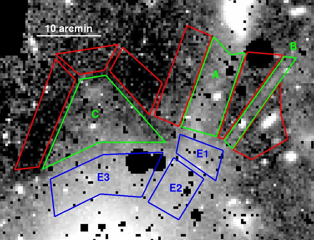
Figure 6.— The area just to the north of M87, containing several interesting tidal features for which we have measured $B-V$ colors. The regions outlined in green – labeled A, B, and C, respectively — are the tidal features themselves. The blue regions — labeled E1, E2, and E3 — are regions within M87’s stellar envelope. The red regions are examples of background regions used to measure the local sky brightness. Discrete objects in the field, such as bright galaxies, are masked during the photometric analysis. Details of the photometric techniques used on these regions are given in the text.

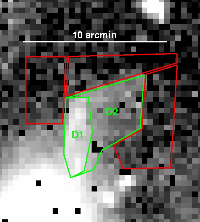
Figure 7.— The plume to the north of the interacting galaxy pair NGC4435/4438. Similar to Figure 6, the green areas — labeled D1 and D2 — enclose the plume itself, while the red regions are used as the local background regions.

While our ability to accurately measure colors is limited over large scales by gradients in the photometric sky levels and extended diffuse light sources, over shorter scales these uncertainties are much smaller. Thus, for smaller scale features, such as individual ICL streams which span $\lower 2.15277pt\hbox{$\;\buildrel<\over{\sim}\;$}10$′, we can use regions adjacent to the features to define the local background flux and more precisely measure luminosities and colors. We have used a differential photometry technique whereby we define object and neighboring background regions, and measure the object luminosity by subtracting the flux in these local background fields. Discrete objects in the fields, such as bright galaxies, are masked so that we are measuring only the diffuse light of the features themselves, and we vary a number of parameters, including the precise placement of region boundaries, in order to estimate the measurement uncertainties (these processes are described in detail in the Appendix). In essence, this technique is a variation on familiar aperture photometry methods used for point sources, where the background flux is measured from an annulus just beyond a circular aperture.

The background regions contain three sources of flux, each of which is also present in the object region and should be removed to isolate the stream’s luminosity. First, as discussed previously, the background regions should share any systematic offset in the sky zero level with the object. Second, in addition to individual tidal streams, the cluster ICL likely contains a large-scale diffuse component which permeates both the object and background regions. Finally, there are numerous foreground and background sources in all the regions; although we attempt to mask these objects (described in the Appendix), because faint sources should be distributed approximately homogeneously on these scales (Brainerd et al. 1995; Villumsen et al. 1997; Connolly et al. 2002; Coil et al. 2004; Morganson & Blandford 2009), their contribution should be equivalent in all regions. We discuss a detailed error budget for this photometric technique in the Appendix.

4.2.1 M87’s Northern Stellar Envelope and Tidal Streams

A number of the most interesting low-surface brightness features in our mosaic occur in the northernmost regions of M87’s extended stellar halo. In particular, Figure 6 highlights three ICL features that we have identified for more detailed study: the large tidal stream extending north-west from M87 toward NGC 4461/4458 (stream A from M05); the smaller stream just to the west which is also emanating from M87 to the northwest (stream B from M05); and the broad plume to the east of these streams, almost directly north of M87’s core (unlabeled in M05, labeled C in Figure 6). Additionally, we have defined three neighboring regions (labeled E1, E2, and E3) which are more clearly part of M87’s outer stellar envelope. In addition to being discussed below, all color measurements for these features can be found in Table 1.

Table 1Photometry of Low-Surface Brightness Features

Region	$B-V$	$\mu_{V}$
(see Figures 6 & 7)		mag arcsec-2
A	0.75-1.05	28.6
B	0.8-1.2	29.2
C	0.7-1.0	28.7
E1	0.8-0.9	28.2
E2	0.75-0.85	27.7
E3	0.75-0.85	27.6
D1	0.65-0.75	27.2
D2	0.5-0.7	28.4

Precisely measuring the colors of these features is quite difficult, and the uncertainties are dominated by numerous systematic effects which are detailed in the Appendix. For this reason, we prefer to quote our measured colors as ranges, rather than as central values with error estimates, which imply a well-characterized Gaussian error model. For features A, B, and C, we measure B V colors of $0.75-1.05$, $0.8-1.2$, and $0.7-1.0$, respectively, with mean surface brightnesses of $\mu_{V}$$\approx 28.6$ mag arcsec^-2, $\mu_{V}$$\approx 29.2$ mag arcsec^-2, $\mu_{V}$$\approx 28.7$ mag arcsec^-2, respectively. If these streams were displayed on the raw color map of Figure 4, however, they would each show a B V color of $\approx 0.5$. This difference in color highlights the difficulty in interpreting the colors of very low surface brightness features from the raw $B-V$ color map and the importance of using a local background subtraction when performing photometric measurements.

Regions E1, E2, and E3 in M87’s stellar envelope display very similar colors to the tidal features. For E1 we measure B V$\approx 0.8-0.9$ with mean surface brightness of $\mu_{V}$$\approx 28.2$, while both E2 and E3 have B V$\approx 0.75-0.85$, with surface brightnesses of $\mu_{V}$$\approx 27.7$ mag arcsec^-2and $\mu_{V}$$\approx 27.6$ mag arcsec^-2, respectively. The measured color ranges are tighter in these regions due to their higher surface brightnesses, meaning that systematic effects have a comparatively smaller effect (see the Appendix for details). Both E2 and E3 lie approximately along the $2000\arcsec$ semi-major axis ellipse around M87, and their colors measured using this differential method agree very well with those of the radial profile, shown in Figure 5, at this radius.

Thus, within the measurement errors, we find that the optical colors of the tidal features are consistent with those of M87’s outer stellar envelope. This suggests that these various features consist of similar stellar populations and may have a common origin. In fact, the colors we measure in these features are also consistent with the optical colors measured for Virgo’s dwarf elliptical galaxy population of B V$\approx 0.8$ (van Zee et al. 2004). The implications of these findings for the evolution of galaxies within the Virgo cluster are discussed in Section 5.

4.2.2 The Plume of NGC 4435/4438

Figure 7 shows another prominent low-surface brightness feature in the Virgo cluster core, the dog-legged plume just to the north of the interacting pair NGC 4435/4438 (feature D from M05). For this plume, we have divided the feature into two sections, the relatively high surface brightness vertical plume, and the lower surface brightness diffuse emission to the west, labeled D1 and D2, respectively, in Figure 7. These features are the bluest in the image for which we have made reliable measurements. We find that D1 has a $B-V$ color of $\approx 0.65-0.75$ with mean surface brightness $\mu_{V}$$\approx 27.1$ mag arcsec^-2 while D2 has $B-V$$\approx 0.5-0.7$ and $\mu_{V}$$\approx 28.4$ mag arcsec^-2.

A wide range of multi-wavelength observations have recently been made of this feature (Cortese et al. 2010; Krick et al. 2010), and its origin — whether a tidal feature from the interaction of NGC 4435/4438 or simply foreground galactic cirrus — is currently in doubt. While its visual morphology is immediately reminiscent of an interaction-induced tidal plume, especially given that NGC 4438 displays obvious signs of tidal disturbance, Cortese et al. (2010) argue that the feature’s UV-IR color and extremely narrow CO and HI velocity widths are more consistent with it being a galactic cirrus dust cloud. If it is truly an extragalactic feature, its blue colors may hint at recent tidally induced star formation, and HST imaging should be able to resolve a young stellar population. If it proves to be a galactic cirrus feature, however, it provides an excellent, if sobering, example of the difficulty of discerning an object’s origin by morphology alone and of the problems that galactic cirrus poses for deep observations of extragalactic objects.

4.2.3 Limits of the Differential Photometry Technique

While our differential photometry technique allows us to increase the precision of our color measurements by more robustly estimating the photometric uncertainties, the procedure’s applicability is often limited by features’ geometry. Most importantly, any features on which we use this technique must have obvious background regions immediately surrounding them, preferably on multiple sides. As detailed in the Appendix, the choice of background region is often the dominant source of systematic uncertainty in a feature’s measured color. This geometric criterion rules out many of the most interesting ICL features seen in our image as candidates for the differential photometry method. For instance, a region of our mosaic displaying a number of interesting low-surface brightness tidal features is the area surrounding M86 and M84, especially the many interacting galaxies to their south. However, because there are numerous overlapping ICL features throughout the region, including both individual tidal streams as well as larger diffuse components, it is extraordinarily difficult to properly define regions in which to measure the background flux for any particular feature, thus limiting our ability to perform accurate photometry of these features.

4.3. Fundamental Photometric Limits

The extremely large color scatter in the azimuthally sliced bins of the outermost regions of M87’s extended stellar halo seen in Figure 5 suggests that we are unable to measure the colors of diffuse light at these very low surface brightnesses with the precision necessary to meaningfully constrain the stellar populations present. We estimate the surface brightness limit to which we can adequately measure colors to be $\mu_{V}$$\approx 27$ mag arcsec^-2 in large, degree-scale features such as the giant elliptical galaxies. While our local background subtraction technique detailed in Section 4.2 is able to substantially reduce the photometric errors for certain features with smaller angular sizes ($\lower 2.15277pt\hbox{$\;\buildrel<\over{\sim}\;$}10$ arcmin), allowing us to push our measurements to lower surface brightnesses, it is not universally applicable to all diffuse light features in the image. Because at the lowest surface brightnesses we are limited by systematic uncertainties in the brightness of both the night sky and astrophysical sources of diffuse light, and not from random statistical noise or known features of the optical design, we may be approaching the fundamental limit of precision available from ground-based, wide-field surface photometry.

While the Virgo cluster is an appealing target in which to study ICL in part because it is the nearest massive galaxy cluster and thus ICL features can be seen over large angular scales, its large angular size actually acts as a hindrance to our ability to perform accurate surface photometry at the faintest levels. As discussed in Section 2.5, even with the Burrell Schmidt’s extremely wide-field imaging capability, the diffuse light features of the Virgo cluster essentially fill the entire field of view, making it extremely difficult to measure and subtract the brightness of the night sky. Thus, we may be able to achieve even greater imaging depth and reduce large-scale uncertainties for targets with smaller angular sizes, such as individual galaxies in the local universe or clusters at higher redshift, where the object does not fill the field of view, and the sky brightness, including large-scale sky gradients, can be more precisely measured.

5. Summary and Discussion

In this paper, we have presented our $B$-band image of the Virgo cluster core, taken as part of our ongoing deep imaging survey of the Virgo cluster. All aspects of the survey, from the optical and mechanical design of the telescope system, to the acquisition, analysis, and reduction of the data have been optimized to detect diffuse light at low surface brightness. Our final photometric uncertainties are dominated by systematic errors resulting from sky subtraction and astrophysical backgrounds and not simple photon statistics.

Our $B$-band imaging confirms the results of M05, which found a vast web of diffuse light features in the core of the Virgo cluster. These features include large-scale diffuse components, as well as a number of discrete features such as streamers, arcs, tails, and plumes which provide a wealth of information on the dynamical history of the cluster and its constituent galaxies. Just outside the cluster core, however, we have detected a large number of galactic cirrus features which prevent us from studying diffuse extragalactic sources which lie behind them.

By combining these $B$-band results with the $V$-band imaging from M05, we have been able to measure the colors of a number of low surface brightness features in Virgo’s core. We have measured the radial color profile of M87 out to very large radius, demonstrating that the color gradients seen in the inner regions of the galaxy extend to its outer stellar envelope. Furthermore, we have measured the colors of several tidal features which extend from M87’s stellar envelope and find that the two populations have similar optical colors within the measurement uncertainties. These results are consistent with the majority of other measurements of ICL color, which suggest that the ICL colors should be similar to those of the outskirts of the cluster’s brightest galaxies (e.g., Zibetti et al. 2005; Sommer-Larsen et al. 2005; Krick & Bernstein 2007).

These results are consistent with the hypothesis that the outer envelopes of cD galaxies like M87 may be predominantly built-up by the tidal stripping and disruption of smaller satellite galaxies, the same mechanism which likely generates the tidal streams and other ICL features (Rudick et al. 2009). In this scenario, the cD envelope is simply composed of tidal streams of ICL which have been mixed in the cluster potential, and dissolved to form a smooth distribution. While optical colors alone cannot definitively prove that any two stellar populations are identical due to the well-known age-metallicity degeneracy, the similar colors of these two populations is suggestive of a common origin.

The optical colors of both the tidal features and M87’s outer envelope are also consistent with the colors of the Virgo cluster’s dwarf elliptical galaxy population (van Zee et al. 2004). Thus, the disruption of these galaxies in the cluster potential may provide a ready source for the intracluster stars which make up the low-surface brightness outer envelope of M87 and the tidal streams. In fact, the thinness of two of the tidal streams studied in Section 4.2.1 suggests that they originate from low-mass galaxies with small velocity dispersions (M05), such as dwarf ellipticals. Furthermore, the results of Williams et al. (2007), who measured the age and metallicity of Virgo’s intracluster stars at much larger radius from any of the cluster’s large galaxies to be $\lower 2.15277pt\hbox{$\;\buildrel>\over{\sim}\;$}10$ Gyr and [M/H]$\lower 2.15277pt\hbox{$\;\buildrel<\over{\sim}\;$}-1.0$, are consistent with the same B V$\approx 0.8$ color that we measure for the streams and stellar envelope immediately beyond M87 (Bruzual & Charlot 2003). This color similarity further bolsters the case that M87’s extended stellar envelope, the tidal streams from disrupted galaxies, and the truly intra-cluster stars all form a single population, formed through similar mechanisms of tidal stripping during the cluster’s hierarchical assembly.

Appendix A Photometric Errors

There are a number of both random and systematic effects which contribute to the uncertainty in our photometric measurements, many of which were mentioned in the main body of the paper. Here, we discuss how these various effects interact to yield our final measurement errors. In general, we find that random errors from photon noise make an insignificant contribution to the error budget, and that the systematic effects which dominate are highly dependent on the angular scales being probed. Below, we calculate the errors from photon statistics to show that they are negligible, and then describe the error sources which predominate in the angular scale regimes discussed in Sections 4.1 and 4.2.

A.1. Small-scale Random Errors

The pixel-to-pixel measurement error based simply on random photon statistics is a straightforward calculation. For a single image with a typical sky value of 750 ADU (because the ICL features we are measuring are $<1\%$ of the sky brightness, we are dominated by sky photons even in our target frames), the photon noise in ADU is given by $\sqrt{C_{s}/g}$, where $C_{s}$ is the sky flux in ADU and $g$ is the gain in $e^{-}$ ADU^-1. For our gain of 2.0$e^{-}$ ADU^-1 this comes to 19.4 ADU pix^-1, or $2.6\%$. When we combine images, however, this error is scaled by a factor of $1.22/\sqrt{N}$, where $N$ is the number of images combined. Our flat field, which contains a minimum of 37 images, thus has an error of $0.52\%$, corresponding to 3.9 ADU pix^-1. In the final mosaic, we further reduce the errors by combining a minimum of five images, for a final error of $0.28\%$, or 2.1 ADU pix^-1. This is, however, an absolute maximum for our random photometric error, and for all measurements made in this paper it is significantly lower.

In the calculation above we assumed the minimum number of five target exposures, whereas $\lower 2.15277pt\hbox{$\;\buildrel>\over{\sim}\;$}30$ exposures are more typical across the image, which reduces the error by another factor of 2.6, or to $<1$ ADU pix^-1. Even greater reductions in the random errors, however, are achieved due to the fact that the diffuse nature of ICL features means that they are spread over a very large number of pixels. Any feature which covers even 100 pixels will have its random photometric error reduced by an order of magnitude. Because the final mosaic shown in Figure 2 has been binned in 16$\times$16 pixel groups, its random per pixel photometric error from photon statistics falls to well below to 0.1 ADU, or $<0.01\%$.

A.2. Large-scale ($\lower 2.15277pt\hbox{$\;\buildrel>\over{\sim}\;$}0.5$°) Systematic Sky Level Uncertainties

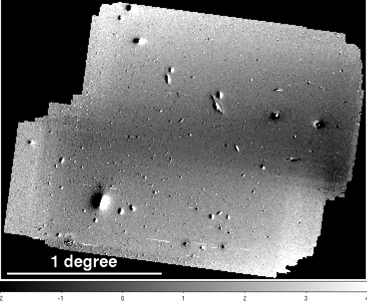
Figure 8.— The difference between the current image using a new sky subtraction technique and the 2005 image, in ADU. The butterfly pattern seen near the centers of bright galaxies is caused by a slight differences in the astrometric calibration of the two images (see Section 4).

As mentioned in Section 2.5, our ability to properly subtract the flux of the night sky from our object images leads to our greatest source of large-scale systematic uncertainty. In that section, we described the two different techniques that we have used to measure the sky signal. Figure 8 shows the difference between our $V$-band images, sky subtracted using the two methods. We expect the large-scale sky level uncertainties in the $V$-band mosaic to be more severe than in the $B$-band, since the $V$-band data was taken using a CCD with only half of the current field of view, meaning that there were even fewer pixels available from which to estimate the sky level gradients. In general, the sky level offset varies smoothly across the field. The largest differences are found in the extreme northeast and southwest corners, where the two images differ by up to 4 ADU, but values of $\approx 1-2$ ADU are much more common. While in certain specific cases, we see that one of the techniques yields unphysical results in certain areas of the image (e.g., the extremely red colors of NGC 4473 and 4477 seen in the northeast corner of Figure 4), we cannot constrain the sky level more generally. Thus, when measuring large-scale features, such as the extended stellar envelope of M87 in Section 4.1, we can only roughly estimate a systematic sky level uncertainty, using the variations seen in Figure 8 as a guide, and recognizing that this is not the only source of systematic uncertainty.

A.3. Intermediate-scale ($\lower 2.15277pt\hbox{$\;\buildrel<\over{\sim}\;$}10$′) Differential Photometry Uncertainties

In Section 4.2 we described the differential photometry technique which we have developed to measure the colors of low-surface brightness features on intermediate scales, such as individual tidal features. Using this method, we can more robustly measure the colors of diffuse light features, resulting in much smaller uncertainties. We have identified four primary contributions to the uncertainty using this technique, each of which behaves in systematic, highly non-Gaussian ways. While the precise magnitude of these effects varies depending on the feature being measured, we use stream A, shown in Figure 6, as an example to illustrate the relative importance of each. For this feature, we find a color of $B-V$$\approx 0.75-1.05$, which might be re-written as $B-V$$=0.9\pm 0.15$.

In order to measure a feature’s color, we need to determine the per pixel flux level of both the object and background regions. These measurements are limited by the uniformity of flux across the regions from astrophysical sources. While in the idealized case of a Gaussian distribution the precision to which we could determine the mean value is given by $\sigma/\sqrt{N}$, which for our data comes to $\approx 0.01$ ADU, the non-Gaussianity of the pixel-values results in a much larger error. We have estimated this uncertainty by using various statistical measures of the per pixel flux, including the assigning the per pixel flux to be the mean or median value. In general, we find that our results are relatively insensitive to the statistical measurement used, and for our example stream this results in a $B-V$ error of $\pm\approx 0.05$ mag.

There are two distinct effects contributing to the photometric uncertainty related to the placement of the object and background regions, respectively. The region boundaries were determined by eye, and are designed to qualitatively select the stream itself and the surrounding background regions where there are no obvious ICL features. In general, defining the object regions was relatively straightforward, and we find that almost any reasonable selection for the regions’ boundaries have a comparatively small effect on the measurement uncertainty, which we estimate to be $\pm\approx 0.05$ mag in the $B-V$ color for our example stream. The uncertainty resulting from selecting various background regions, however, has a profound effect on the measured colors, and is often the single largest source of error. Each background region has a slightly different flux level due to any small-scale sky level gradients or very faint diffuse light features present. Because the objects we are measuring have such low surface brightnesses, even small differences in the background flux levels result in large errors in the colors. For our example feature we estimate the uncertainty due to background region selection to be $\pm\approx 0.15$ mag in $B-V$. This uncertainty from the selection of background regions stems primarily from using regions on different areas of the sky, whereas adjusting the precise borders of a background region has a comparatively small effect.

The final component of the color uncertainty comes from our treatment of foreground/background sources which, of course, permeate the image. Ideally, any method we use to mask these sources should result in a negligible change in the color since it should affect all regions equally, and faint sources are expected to be unclustered on these scales (e.g., Brainerd et al. 1995). We have used two methods to eliminate the luminosity from bright sources. In the first, we ran objmask to mask all objects in the image; our final mask combined all objects detected in either the $V$ or $B$ images. Alternatively, we used only a $\sigma$-clipping algorithm to remove high-intensity pixels. We notice a systematic offset in the colors using these two masking procedures where the objmask technique produces redder $B-V$ colors by $\approx 0.1$ mag. Unfortunately, using objmask to mask sources becomes unfeasible at flux levels much above 5 ADU ($\approx 27.5$ mag arcsec^-2), as the features we are measuring are themselves masked.

Each feature’s final quoted color range takes into account all of these effects by making numerous measurements while systematically varying the input parameters. While we can estimate the uncertainties caused by each of these four effects, they are all systematic and interdependent sources of error, and thus not subject to the usual methods of error propagation. We quote the final measured colors as ranges to emphasize the non-Gaussianity of the errors, especially given the fact that our results are often not consistent with a central measured value.

Although this paper is focused almost exclusively on the color of ICL features, and not their total luminosity or mean surface brightness, this differential photometry method is also suitable for measuring those quantities, and mean surface brightness is given for each feature in the text. One interesting detail that we find when we calculate these quantities is that the uncertainty in the color measurement is smaller than the uncertainty in mean surface brightness in either band; i.e., we can measure the ratio of the fluxes in the two bands more precisely than we can measure the absolute flux in either band. This peculiar effect arises from the fact that the dominant source of error in this photometric technique is the choice of background region. Because the variation between background regions is caused predominantly by changes in the flux level of astrophysical backgrounds, such as large-scale ICL components, the flux in these background regions is correlated in the two bands, and the mean surface brightness measurements are not independent of one another. This odd behavior of the photometric uncertainties once again illustrates that because our measurements are truly limited by astrophysical backgrounds, the resulting errors are highly systematic and non-Gaussian.

References

- Abadi et al. (2006) Abadi, M. G., Navarro, J. F., & Steinmetz, M. 2006, MNRAS, 365, 747
- Adami et al. (2005) Adami, C., et al. 2005, A&A, 429, 39
- Aguerri et al. (2005) Aguerri, J. A. L., Gerhard, O. E., Arnaboldi, M., Napolitano, N. R., Castro-Rodriguez, N., & Freeman, K. C. 2005, AJ, 129, 2585
- Arnaboldi et al. (2004) Arnaboldi, M., Gerhard, O., Aguerri, J. A. L., Freeman, K. C., Napolitano, N. R., Okamura, S., & Yasuda, N. 2004, ApJ, 614, L33
- Baria et al. (2009) Baria, P., Brito, W., & Martel, H. 2009, Journal of Astrophysics and Astronomy, 30, 1
- Bernardi et al. (2003) Bernardi, M., et al. 2003, AJ, 125, 1882
- Bernstein et al. (1995) Bernstein, G. M., Nichol, R. C., Tyson, J. A., Ulmer, M. P., & Wittman, D. 1995, AJ, 110, 1507
- Brainerd et al. (1995) Brainerd, T. G., Smail, I., & Mould, J. 1995, MNRAS, 275, 781
- Bruzual & Charlot (2003) Bruzual, G., & Charlot, S. 2003, MNRAS, 344, 1000
- Calcáneo-Roldán et al. (2000) Calcáneo-Roldán, C., Moore, B., Bland-Hawthorn, J., Malin, D., & Sadler, E. M. 2000, MNRAS, 314, 324
- Cantiello et al. (2005) Cantiello, M., Blakeslee, J. P., Raimondo, G., Mei, S., Brocato, E., & Capaccioli, M. 2005, ApJ, 634, 239
- Carollo et al. (1993) Carollo, C. M., Danziger, I. J., & Buson, L. 1993, MNRAS, 265, 553
- Carter & Dixon (1978) Carter, D., & Dixon, K. L. 1978, AJ, 83, 574
- Castro-Rodriguéz et al. (2009) Castro-Rodriguéz, N., Arnaboldi, M., Aguerri, J. A. L., Gerhard, O., Okamura, S., Yasuda, N., & Freeman, K. C. 2009, A&A, 507, 621
- Coil et al. (2004) Coil, A. L., Newman, J. A., Kaiser, N., Davis, M., Ma, C.-P., Kocevski, D. D., & Koo, D. C. 2004, ApJ, 617, 765
- Connolly et al. (2002) Connolly, A. J., et al. 2002, ApJ, 579, 42
- Conroy et al. (2007) Conroy, C., Wechsler, R. H., & Kravtsov, A. V. 2007, ApJ, 668, 826
- Cortese et al. (2010) Cortese, L., Bendo, G. J., Isaak, K. G., Davies, J. I., & Kent, B. R. 2010, MNRAS, 403, L26
- Da Rocha & Mendes de Oliveira (2005) Da Rocha, C., & Mendes de Oliveira, C. 2005, MNRAS, 364, 1069
- Da Rocha et al. (2008) Da Rocha, C., Ziegler, B. L., & Mendes de Oliveira, C. 2008, MNRAS, 388, 1433
- Davis et al. (1985) Davis, L. E., Cawson, M., Davies, R. L., & Illingworth, G. 1985, AJ, 90, 169
- de Vaucouleurs (1961) de Vaucouleurs, G. 1961, ApJS, 5, 233
- Dubinski (1998) Dubinski, J. 1998, ApJ, 502, 141
- Durrell et al. (2002) Durrell, P. R., Ciardullo, R., Feldmeier, J. J., Jacoby, G. H., & Sigurdsson, S. 2002, ApJ, 570, 119
- Faure et al. (2007) Faure, C., Giraud, E., Melnick, J., Quintana, H., Selman, F., & Wambsganss, J. 2007, A&A, 463, 833
- Feldmeier et al. (1998) Feldmeier, J. J., Ciardullo, R., & Jacoby, G. H. 1998, ApJ, 503, 109
- Feldmeier et al. (2004) Feldmeier, J. J., Ciardullo, R., Jacoby, G. H., & Durrell, P. R. 2004, ApJ, 615, 196
- Feldmeier et al. (2004) Feldmeier, J. J., Mihos, J. C., Morrison, H. L., Harding, P., Kaib, N., & Dubinski, J. 2004, ApJ, 609, 617
- Feldmeier et al. (2002) Feldmeier, J. J., Mihos, J. C., Morrison, H. L., Rodney, S. A., & Harding, P. 2002, ApJ, 575, 779
- Ferguson et al. (1998) Ferguson, H. C., Tanvir, N. R., & von Hippel, T. 1998, Nature, 391, 461
- Gal-Yam et al. (2003) Gal-Yam, A., Maoz, D., Guhathakurta, P., & Filippenko, A. V. 2003, AJ, 125, 1087
- Gerhard et al. (2005) Gerhard, O., Arnaboldi, M., Freeman, K. C., Kashikawa, N., Okamura, S., & Yasuda, N. 2005, ApJ, 621, L93
- Gnedin (2003) Gnedin, O. Y. 2003, ApJ, 582, 141
- Gonzalez et al. (2005) Gonzalez, A. H., Zabludoff, A. I., & Zaritsky, D. 2005, ApJ, 618, 195
- Gonzalez et al. (2000) Gonzalez, A. H., Zabludoff, A. I., Zaritsky, D., & Dalcanton, J. J. 2000, ApJ, 536, 561
- Goudfrooij et al. (1994) Goudfrooij, P., Hansen, L., Jorgensen, H. E., Norgaard-Nielsen, H. U., de Jong, T., & van den Hoek, L. B. 1994, A&AS, 104, 179
- Gregg & West (1998) Gregg, M. D., & West, M. J. 1998, Nature, 396, 549
- Guhathakurta & Tyson (1989) Guhathakurta, P., & Tyson, J. A. 1989, ApJ, 346, 773
- Krick & Bernstein (2007) Krick, J. E., & Bernstein, R. A. 2007, AJ, 134, 466
- Krick et al. (2006) Krick, J. E., Bernstein, R. A., & Pimbblet, K. A. 2006, AJ, 131, 168
- Krick et al. (2010) Krick, J., et al. 2010, Bulletin of the American Astronomical Society, 41, 588
- Lang et al. (2010) Lang, D., Hogg, D. W., Mierle, K., Blanton, M., & Roweis, S. 2010, AJ, 139, 1782
- Liu et al. (2005) Liu, Y., Zhou, X., Ma, J., Wu, H., Yang, Y., Li, J., & Chen, J. 2005, AJ, 129, 2628
- Maoz et al. (2005) Maoz, D., Waxman, E., & Loeb, A. 2005, ApJ, 632, 847
- McGee & Balogh (2010) McGee, S. L., & Balogh, M. L. 2010, MNRAS, 403, L79
- Mihos et al. (2005) Mihos, J. C., Harding, P., Feldmeier, J., & Morrison, H. 2005, ApJ, 631, L41
- Monaco et al. (2006) Monaco, P., Murante, G., Borgani, S., & Fontanot, F. 2006, ApJ, 652, L89
- Moore et al. (1996) Moore, B., Katz, N., Lake, G., Dressler, A., & Oemler, A. 1996, Nature, 379, 613
- Morganson & Blandford (2009) Morganson, E., & Blandford, R. 2009, MNRAS, 398, 769
- Murante et al. (2004) Murante, G., et al. 2004, ApJ, 607, L83
- Murante et al. (2007) Murante, G., Giovalli, M., Gerhard, O., Arnaboldi, M., Borgani, S., & Dolag, K. 2007, MNRAS, 377, 2
- Napolitano et al. (2003) Napolitano, N. R., et al. 2003, ApJ, 594, 172
- Neill et al. (2005) Neill, J. D., Shara, M. M., & Oegerle, W. R. 2005, ApJ, 618, 692
- Pettit (1954) Pettit, E. 1954, ApJ, 120, 413
- Pierini et al. (2008) Pierini, D., Zibetti, S., Braglia, F., Böhringer, H., Finoguenov, A., Lynam, P. D., & Zhang, Y.-Y. 2008, A&A, 483, 727
- Purcell et al. (2008) Purcell, C. W., Bullock, J. S., & Zentner, A. R. 2008, MNRAS, 391, 550
- Purcell et al. (2007) Purcell, C. W., Bullock, J. S., & Zentner, A. R. 2007, ApJ, 666, 20
- Rawle et al. (2010) Rawle, T. D., Smith, R. J., & Lucey, J. R. 2010, MNRAS, 401, 852
- Rudick et al. (2006) Rudick, C. S., Mihos, J. C., & McBride, C. 2006, ApJ, 648, 936
- Rudick et al. (2009) Rudick, C. S., Mihos, J. C., Frey, L. H., & McBride, C. K. 2009, ApJ, 699, 1518
- Ruszkowski & Springel (2009) Ruszkowski, M., & Springel, V. 2009, ApJ, 696, 1094
- Sánchez-Blázquez et al. (2007) Sánchez-Blázquez, P., Forbes, D. A., Strader, J., Brodie, J., & Proctor, R. 2007, MNRAS, 377, 759
- Sandage (1976) Sandage, A. 1976, AJ, 81, 954
- Schlegel et al. (1998) Schlegel, D. J., Finkbeiner, D. P., & Davis, M. 1998, ApJ, 500, 525
- Slater et al. (2009) Slater, C. T., Harding, P., & Mihos, J. C. 2009, PASP, 121, 1267
- Sommer-Larsen et al. (2005) Sommer-Larsen, J., Romeo, A. D., & Portinari, L. 2005, MNRAS, 357, 478
- Spinrad et al. (1972) Spinrad, H., Smith, H. E., & Taylor, D. J. 1972, ApJ, 175, 649
- Strom et al. (1976) Strom, S. E., Strom, K. M., Goad, J. W., Vrba, F. J., & Rice, W. 1976, ApJ, 204, 684
- Strom & Strom (1978) Strom, K. M., & Strom, S. E. 1978, AJ, 83, 73
- Tamura et al. (2000) Tamura, N., Kobayashi, C., Arimoto, N., Kodama, T., & Ohta, K. 2000, AJ, 119, 2134
- Trentham & Mobasher (1998) Trentham, N., & Mobasher, B. 1998, MNRAS, 293, 53
- Uson et al. (1991) Uson, J. M., Boughn, S. P., & Kuhn, J. R. 1991, ApJ, 369, 46
- Vader et al. (1988) Vader, J. P., Vigroux, L., Lachieze-Rey, M., & Souviron, J. 1988, A&A, 203, 217
- van Zee et al. (2004) van Zee, L., Barton, E. J., & Skillman, E. D. 2004, AJ, 128, 2797
- Vilchez-Gomez et al. (1994) Vilchez-Gomez, R., Pello, R., & Sanahuja, B. 1994, A&A, 283, 37
- Villumsen et al. (1997) Villumsen, J. V., Freudling, W., & da Costa, L. N. 1997, ApJ, 481, 578
- White et al. (2003) White, P. M., Bothun, G., Guerrero, M. A., West, M. J., & Barkhouse, W. A. 2003, ApJ, 585, 739
- Williams et al. (2007) Williams, B. F., et al. 2007, ApJ, 656, 756
- Willman et al. (2004) Willman, B., Governato, F., Wadsley, J., & Quinn, T. 2004, MNRAS, 355, 159
- Witt et al. (2008) Witt, A. N., Mandel, S., Sell, P. H., Dixon, T., & Vijh, U. P. 2008, ApJ, 679, 497
- Yagi et al. (2007) Yagi, M., Komiyama, Y., Yoshida, M., Furusawa, H., Kashikawa, N., Koyama, Y., & Okamura, S. 2007, ApJ, 660, 1209
- Zeilinger et al. (1993) Zeilinger, W. W., Moller, P., & Stiavelli, M. 1993, MNRAS, 261, 175
- Zibetti et al. (2005) Zibetti, S., White, S. D. M., Schneider, D. P., & Brinkmann, J. 2005, MNRAS, 358, 949
- Zwicky (1951) Zwicky, F. 1951, PASP, 63, 61