A Discontinuous Galerkin Method for Ideal Two-Fluid Plasma Equations

Abstract

A discontinuous Galerkin method for the ideal 5 moment two-fluid plasma system is presented. The method uses a second or third order discontinuous Galerkin spatial discretization and a third order TVD Runge-Kutta time stepping scheme. The method is benchmarked against an analytic solution of a dispersive electron acoustic square pulse as well as the two-fluid electromagnetic shock [1] and existing numerical solutions to the GEM challenge magnetic reconnection problem [2]. The algorithm can be generalized to arbitrary geometries and three dimensions. An approach to maintaining small gauge errors based on error propagation is suggested.

1 Introduction

Fusion power promises to be a safe, efficient and environmentally friendly energy source. Controlled fusion power concepts have been under investigation for decades, the vast majority of these concepts require an intimate understanding of plasma physics to determine the stability and confinement properties. Numerical plasma physics has proved extremely valuable in deciphering experimental data and predicting the behavior of plasma experiments. Many plasma fluid models, and in particular the full two-fluid plasma model, have received very little attention from the numerical plasma physics community. This work describes an advanced algorithm for the ideal 5-moment two-fluid plasma system.

To solve problems in plasma physics and to gain physical intuition of plasma phenomena a hierarchy of classical plasma models have been developed. The most fundamental continuum plasma model is the Vlasov model which eliminates individual particles in favor of a continuous distribution function. This model is six dimensional as the distribution function is a function of both position and velocity. The Vlasov model can be re-written as an equivalent system that consists of an infinite number of moment equations. A reduction of the Vlasov model can then be obtained by truncating this infinite series. Assuming scalar pressure and setting the heat tensor and higher moments to zero produces the 5 moment truncation of the Vlasov model. This model is known as the ideal 5 moment two-fluid plasma model, and will be discussed in this paper. Asymptotic approximations of this two-fluid system produce a series of increasingly simpler fluid models including two-fluid MHD (Magnetohydrodynamics), Hall MHD and then the ideal MHD models.

The main benefit of a fluid model over the Vlasov model is the reduced dimensionality from 6 dimensions to 3 dimensions. Physics is lost in this reduction, but an enormous amount of physics relevant to fusion and spacecraft propulsion remains in the fluid description. Ideal MHD has been extremely successful in explaining large scale instabilities in such devices as the Z-pinch, spheromak and tokamak [3, 4]. Unfortunately there are many regimes where the description is invalid and where it fails to explain the observed phenomena. An example of this includes ion demagnetization which is important in Field Reversed Configurations [5] and Hall thrusters. Hall MHD addresses both these issues but fails to describe other plasma phenomena such as the demagnetization of electrons in regions of low magnetic field which is important in collisionless reconnection. The two-fluid MHD approach adds terms such as electron inertia which is an important mechanism for breaking the frozen in flux condition for electrons as it acts as a “dissipation” mechanism in the absence of resistivity [6]. The quasi-neutrality condition still constrains the electron and ion motions, to allow complete independence of electron and ion motion the quasi-neutrality condition must be relaxed; the result is the ideal two-fluid plasma system.

Two-fluid effects are important in the generation of turbulence through microinstabilities. Most plasmas are turbulent at some scale, however the simplest fluid model, ideal MHD, describes plasmas physics that is more or less laminar where the two-fluid model produces turbulent phenomena. This can be explained in part by the fluid description of electrons. In a two-fluid model both the electrons and the ions may become unstable independently. In particular, electrons carry most of the current in an MHD plasma. This current may produce a large amount of differential motion in the electron fluid when magnetic field gradients are present even if the plasma is in a static MHD equilibrium. The generation of microturbulence through processes such as the lower hybrid drift instability and the modified two-stream instability may be important in both Z-pinch and theta-pinch plasmas. These instabilities are frequently cited as sources of anomalous resistivity [7], magnetic diffusion and heating and in certain cases may ultimately drive macroscopic MHD instabilities [8].

A particularly good application of the two-fluid plasma model is the fusion Z-pinch [9]. Many plasma experiments last a few seconds whereas the shortest plasma times scale, the electron plasma oscillation, can occur on the scale of pico seconds. However, in the case of the fusion Z-pinch these time scales can be compressed to about 4 orders of magnitude between the shortest time scale, the electron plasma period the MHD instability growth time, which puts two-fluid Z-pinch simulations in the range of numerical methods. Conceptual Z-pinch fusion reactors are high density with extremely strong magnetic fields which makes the two-fluid plasma system particularly applicable [10]. Furthermore the radius of the pinch can be  1000 Debye lengths in some designs [11] which means Debye length scales could be resolved in very high resolution simulations. Artificially increasing the electron mass to ion mass ratio and increasing the ratio of the Alfven speed to the speed of light can make the Z-pinch problem more computationally tractable while maintaining the relevant physics. The analysis of microinstabilities such as the lower hybrid drift instability may be important in progressing towards a better understanding of Z-pinch physics.

Algorithms have been designed for various fluid plasma models including MHD [12, 13], Hall MHD [14, 15, 16, 17] various forms of electrostatic two-fluid plasma models [18, 19, 20] and the ideal two-fluid system [21, 22, 1]. The first well described two-fluid plasma algorithm was the ANTHEM [21, 22] code. It was used to simulate fast phenomena in high density plasmas inaccessible to PIC codes, the applications included simulations of plasma opening switches and the fast igniter concept. ANTHEM used a flux corrected transport (FCT) type algorithm for the fluids and an FDTD type algorithm for the fields. This type of algorithm is difficult to extend to general geometries because of the staggered scheme used for Maxwell’s equations. In [1] a full two-fluid algorithm using the finite volume method for both fluids and fields was described for one-dimensional problems. An issue with the finite volume algorithm was the decay of equilibrium solutions due to the low order of accuracy which resulted from the source term integration and diffusive limiters used. Major improvements on the finite volume technique have been made with the help of various divergence cleaning techniques and careful attention to source term treatment. An improved finite volume approach is described in [23].

The purpose of the paper is to develop a numerical algorithm for the ideal 5 moment two-fluid plasma system using the discontinuous Galerkin method so that it can be easily generalized to arbitrary geometries and to arbitrarily high order accuracy to help capture plasma instabilities. TVB discontinuous Galerkin methods are described in [24, 25, 26]. They are extended to the multi-dimensional Euler equations in [27] and to Maxwell’s equations in [28, 29]. The two-fluid system of equations consists of two sets of Euler equations, one for the electrons and the other for the ions, and the complete Maxwell’s equations. The ideal two-fluid system differs from the ideal MHD equations in that it is composed of three separate (but well understood) hyperbolic systems coupled through source terms. The MHD equations are, on the other hand, a unique hyperbolic system. A discontinuous Galerkin method for the MHD equations was developed in [30] and for two temperature MHD in [31]. The technique is used in a Vlasov-Maxwell algorithm in [32], numerous other applications can be found in [33].

In section 2 the ideal 5-moment two-fluid model is described and the equations are presented. In section 3 a scalar model problem is derived from the two-fluid systems which helps to illustrate some of the numerical issues with the system. In section 4 the discontinuous Galerkin method applied to the two-fluid plasma system is presented. In section 5 simulations are presented including an electron acoustic pulse for validation of code accuracy, an electrostatic shock, the two-fluid electromagnetic shock [1], and the GEM challenge magnetic reconnection problem [2] where the reconnected magnetic flux can be compared to published results. Finally, in section 6 the conclusions are discussed.

2 Two-Fluid Model

The full two-fluid plasma model consists of a set of fluid equations for the electrons and ions plus the complete Maxwell’s equations including displacement current. The fluid and electromagnetic systems are coupled by Lorentz forces and current sources. In the following equations, $\mathbf{E}$ is the electric field, $\mathbf{B}$ is the magnetic field, $q_{s}$ is the species charge (subscript $s$ is $i$ for ions and $e$ for electrons), $\rho_{s}$ is the species density, $m_{s}$ is the species mass, $\mathbf{U}_{s}$ is the species velocity, $P_{s}$ is the species pressure and $e_{s}$ is the species total energy with $e_{s}=\frac{1}{2}\rho_{s}\,\mathbf{U}_{s}^{2}+\frac{1}{1-\gamma_{s}}p_{s}$. The species number density is defined as $n_{s}=\frac{\rho_{s}}{m_{s}}$, $\epsilon_{0}$ is the permittivity and $\mu_{0}$ is the permeability of free space. Maxwell’s equations are presented in SI units. The complete Ampere’s law is used

$$\partial_{t}\,\mathbf{E}-c^{2}\left(\nabla\times\,\mathbf{B}\right)=-\frac{1}{\epsilon_{0}}\sum_{s}\frac{q_{s}}{m_{s}}\rho_{s}\mathbf{U}_{s}\,,$$ (1)

and the complete Faraday’s law

$$\partial_{t}\,\mathbf{B}+\left(\nabla\times\,\mathbf{E}\right)=0\,.$$ (2)

The magnetic flux equation,

$$\nabla\cdot\mathbf{B}=0$$ (3)

and Poisson’s equation (4),

$$\nabla\cdot\mathbf{E}=\frac{1}{\epsilon_{0}}\left(q_{i}\,n_{i}+q_{e}\,n_{e}\right)$$ (4)

are constraint equations which can be derived from Ampere’s law (1), Faraday’s law (2) as well as the species continuity equation given below in (11) under the assumption that the constraints are satisfied initially. A simple way to reduce the error in the constraint equations is to use the perfectly hyperbolic Maxwell’s equations where equations (1), (2), (3), (4) are modified, so that Ampere’s law becomes

$$\partial_{t}\,\mathbf{E}-c^{2}\left(\nabla\times\,\mathbf{B}\right)+\nabla\psi_{E}=-\frac{1}{\epsilon_{0}}\sum_{s}\frac{q_{s}}{m_{s}}\rho_{s}\mathbf{U}_{s}\,,$$ (5)

Faraday’s law becomes

$$\partial_{t}\,\mathbf{B}+\left(\nabla\times\,\mathbf{E}\right)+\nabla\psi_{B}=0\,.$$ (6)

The magnetic flux equation becomes,

$$\frac{1}{\Gamma_{B}^{2}}\frac{\partial\psi_{B}}{\partial t}+\nabla\cdot\mathbf{B}=0$$ (7)

and Poisson’s equation becomes,

$$\frac{1}{\Gamma_{E}^{2}}\frac{\partial\psi_{E}}{\partial t}+\nabla\cdot\mathbf{E}=\frac{1}{\epsilon_{0}}\left(q_{i}\,n_{i}+q_{e}\,n_{e}\right)\,.$$ (8)

Where $\psi_{B}$ and $\psi_{E}$ are correction potentials and $\Gamma_{B}$, $\Gamma_{E}$ are the correction potential wave speeds which propagate errors in the divergence constraints out at the speeds $\Gamma_{B}$ and $\Gamma_{E}$. The correction potential wave speeds can be set to zero for problems where the correction terms are not necessary. Details of the correction potential technique are described in [34] and used in our previous work [23]. In many problems of experimental interest electrons flow from a surface into the simulation domain. In these situations we believe more sophisticate divergence preservation will be required. It’s important to maintain exact charge conservation especially when the emission is space charge limited. For this type of problem a constrained transport approach should be taken. Charge conserving constrained transport is frequently used in particle in cell (PIC) codes [35], [36], [37]. In addition, $\nabla\cdot B=0$ preserving constrained transport is frequently used in the MHD system [38], [39], [40], [41].

The fluid equations are simply the inviscid Navier Stokes equations with Lorentz force source terms. Each fluid species has its own equation for energy,

$$\partial_{t}\,e_{s}+\nabla\cdot\left(\mathbf{U}_{s}\left(e_{s}+P_{s}\right)\right)=\frac{q_{s}}{m_{s}}\rho_{s}\mathbf{E}\cdot\mathbf{U}_{s}\,,$$ (9)

momentum,

$$\partial_{t}\,\left(\rho_{s}\mathbf{U}_{s}\right)+\nabla_{\alpha}\left(\rho_{s}\mathbf{U}_{s}^{\alpha}\mathbf{U}_{s}\right)+\nabla_{\alpha}\left(\delta^{\alpha\,\beta}P_{s}\right)=\frac{q_{s}}{m_{s}}\,\rho_{s}\left(\mathbf{E}+\mathbf{U}_{s}\times\,\mathbf{B}\right)\,,$$ (10)

and continuity,

$$\partial_{t}\,\rho_{s}+\nabla\cdot\left(\rho_{s}\mathbf{U}_{s}\right)=0\,.$$ (11)

This means that each species has its own temperature, velocity and number density. As a result, quasi-neutrality is not assumed and things like electron plasma waves and ion subshocks should be observed numerically. This system is identical to the system used in [1].

The ideal two fluid plasma system can be written as three systems of balance laws,

$$\frac{\partial\,Q_{e}}{\partial t}+\nabla\cdot F_{e}\left(Q_{e}\right)=\psi_{e}\left(Q_{e},\,Q_{em}\right)\,,$$ (12)

for the electron equations,

$$\frac{\partial\,Q_{i}}{\partial t}+\nabla\cdot F_{i}\left(Q_{i}\right)=\psi_{i}\left(Q_{i},\,Q_{em}\right)\,,$$ (13)

for the ion equations, and

$$\frac{\partial\,Q_{em}}{\partial t}+\nabla\cdot F_{em}\left(Q_{em}\right)=\psi_{em}\left(Q_{i},\,Q_{e}\right),$$ (14)

for Maxwell’s equations. These balance laws, Eqns.(12)-(14), are given in full form by,

$$\frac{\partial}{\partial\,t}\left(\begin{array}[]{c}\rho_{s}\\ \rho_{s}\,U_{x\,s}\\ \rho_{s}\,U_{y\,s}\\ \rho_{s}\,U_{z\,s}\\ e_{s}\end{array}\right)+\nabla\cdot\left(\begin{array}[]{ccc}\rho_{s}\,U_{x\,s}&\rho_{s}\,U_{y\,s}&\rho_{s}\,U_{z\,s}\\ \rho_{s}\,U_{x\,s}U_{x\,s}+P_{s}&\rho_{s}\,U_{x\,s}\,U_{y\,s}&\rho_{s}\,U_{x\,s}\,U_{z\,s}\\ \rho_{s}\,U_{y\,s}U_{x\,s}&\rho_{s}\,U_{y\,s}\,U_{y\,s}+P_{s}&\rho_{s}\,U_{y\,s}\,U_{z\,s}\\ \rho_{s}\,U_{z\,s}U_{x\,s}&\rho_{s}\,U_{z\,s}\,U_{y\,s}&\rho_{s}\,U_{z\,s}\,U_{z\,s}+P_{s}\\ U_{x\,s}\left(e_{s}+P_{s}\right)&U_{y\,s}\left(e_{s}+P_{s}\right)&U_{z\,s}\left(e_{s}+P_{s}\right)\\ \end{array}\right)=\\ \left(\begin{array}[]{c}0\\ q_{s}\,n_{s}\left(E_{x}+U_{y\,s}\,B_{z}-U_{z\,s}\,B_{y}\right)\\ q_{s}\,n_{s}\left(E_{y}+U_{z\,s}\,B_{x}-U_{x\,s}\,B_{z}\right)\\ q_{s}\,n_{s}\left(E_{z}+U_{x\,s}\,B_{y}-U_{y\,s}\,B_{x}\right)\\ q_{s}\,n_{s}\left(E_{x}\,U_{x\,s}+E_{y}\,U_{y\,s}+E_{z}\,U_{z\,s}\right)\\ \end{array}\right)$$ (15)

$$\frac{\partial}{\partial t}\left(\begin{array}[]{c}B_{x}\\ B_{y}\\ B_{z}\\ E_{x}\\ E_{y}\\ E_{z}\end{array}\right)+\nabla\cdot\,\left(\begin{array}[]{ccc}0&E_{z}&-E_{y}\\ -E_{z}&0&E_{x}\\ E_{y}&-E_{x}&0\\ 0&-c^{2}\,B_{z}&c^{2}\,B_{y}\\ c^{2}\,B_{z}&0&-c^{2}\,B_{x}\\ -c^{2}\,B_{y}&c^{2}\,B_{x}&0\\ \end{array}\right)=\\ \left(\begin{array}[]{c}0\\ 0\\ 0\\ -\frac{1}{\epsilon_{0}}\left(q_{e}\,n_{e}\,U_{x\,e}+q_{i}\,n_{i}\,U_{x\,i}\right)\\ -\frac{1}{\epsilon_{0}}\left(q_{e}\,n_{e}\,U_{y\,e}+q_{i}\,n_{i}\,U_{y\,i}\right)\\ -\frac{1}{\epsilon_{0}}\left(q_{e}\,n_{e}\,U_{z\,e}+q_{i}\,n_{i}\,U_{z\,i}\right)\\ \end{array}\right)$$ (16)

3 Derivation of a Scalar Model Problem

The ideal 5-moment two-fluid system is unusual in that the source terms act as harmonic oscillators, the source terms are purely dispersive without dissipation or amplification. This fact is important when considering numerical methods to use, as the source term integration should introduce as little dissipation as feasible in order to avoid damping these oscillations. It frequently occurs in a two-fluid plasma that convective forces are in balance with oscillating sources to produce an equilibrium. With this in mind, a simple model problem is derived which may help one choose a proper numerical method for the two-fluid system.

Linearizing the electron x-momentum equation (10) and Ampere’s law (1) while assuming a constant background ion density and assuming that $\mathbf{B}=0$, a partial differential equation for electron plasma oscillations can be derived which takes the form

$$\frac{\partial^{2}u}{\partial\,t^{2}}=-\omega_{p\,e}^{2}u\,,$$ (17)

where $u$ is the perturbed x velocity and $\omega_{p\,e}$ is the electron plasma frequency. This can be transformed to a first order equation in complex variables by making the transformation $\omega_{pe}v=\frac{\partial u}{\partial t}$ and letting $Q=v+i\,u$.

$$\frac{\partial\,Q}{\partial\,t}=i\,\omega_{p\,e}Q\,.$$ (18)

By transforming variables $Q\left(x,t\right)\to Q\left(\eta,t\right)$ where $\eta=x+a\,t$, Equation(18) becomes an advection oscillation equation

$$\frac{\partial Q}{\partial t}+a\frac{\partial Q}{\partial\eta}=i\,\omega_{p\,e}\,Q\,,$$ (19)

where $a$ is the wave propagation speed and $\omega_{p\,e}$ is the oscillation frequency. Any algorithm that is stable to the two-fluid system should be stable when applied to Eqn(19). This equation has solutions $Q=A\,e^{i\left(k\,\eta-\omega\,t\right)}$ where $\omega=a\,k-\omega_{p\,e}$. In particular(19) admits a steady state solution $Q=A\,e^{i\,k\,\eta}$ on an infinite domain where the source term is in balance with the flux. It is important to note that there are an infinite number of equilibria which differ by a continuous range of scalar factors $A$. This point is important when considering numerical methods for this system since a numerical method with too much dissipation could conceivably move a steady state solution from one equilibrium to another all the while moving towards a state where $A=0$. This loss of amplitude is also observed in equilibrium type problems in the two-fluid system. An effective numerical algorithm must be both stable to the advection equation and oscillation equation and must have low dissipation in equilibrium type problems. The discontinuous Galerkin method is an ideal candidate for solving the two-fluid system. Its accuracy can easily be increased to reduce numerical dissipation while being stable to both the advection equation and the oscillation equation.

4 Runge-Kutta Discontinuous Galerkin Method

Discontinuous Galerkin methods are high order extensions of upwind schemes using a finite element formulation where the elements are discontinuous at cell interfaces. Details of the method are discussed in [24, 25, 26, 27] and reproduced here for our particular case. The balance law

$$\frac{\partial Q}{\partial t}+\nabla\cdot F\left(Q\right)=\psi\left(Q\right)$$ (20)

is multiplied by the set of basis functions $\{v_{r}\}$ and integrated over the finite volume element $K$. For second order spatial accuracy the basis set on a unit square reference element is

$$\{v_{r}\}=\{v_{0},v_{x},v_{y}\}=\{1,x,y\}\,.$$ (21)

For third order spatial accuracy

$$\{v_{r}\}=\{v_{0},v_{x},v_{y},v_{x\,y},v_{x\,x},v_{y\,y}\}=\{1,x,y,x\,y,x^{2}-\frac{1}{3},y^{2}-\frac{1}{3}\}$$ (22)

is used. The equation is written,

$$\int_{K}\frac{\partial Q}{\partial t}\,v_{r}\,dV+\int_{K}\left(\nabla\cdot F\right)\,v_{r}\,dV=\int_{K}\psi\,v_{r}\,dV\,.$$ (23)

Integrate by parts to get

$$\int_{K}\frac{\partial Q}{\partial t}\,v_{r}\,dV+\int_{\partial\,K}\left(\tilde{F}\cdot n\right)\,v_{r}\,d\Gamma-\int_{K}F\cdot\left(\nabla\,v_{r}\right)\,dV=\int_{K}\psi\,v_{r}\,dV\,.$$ (24)

The surface flux $\tilde{F}\cdot n$ is a numerical approximation of the exact flux $F\cdot n$ across the interface. The discrete conserved variable $Q$ is defined as a linear combination of the basis functions inside an element $K$, with

$$Q=\sum_{r}\,v_{r}\,Q_{r}\,.$$ (25)

The integral $\int_{K}\frac{\partial Q}{\partial t}\,v_{r}\,dV=\frac{\partial Q_{r}}{\partial t}\,C\,V$ where $C$ is the constant $\frac{1}{V}\int_{K}\,v_{r}^{2}\,dV$ and V is the volume of the element. Using these definitions we get the discrete equation

$$\frac{\partial Q_{r}}{\partial t}C\,V+\sum_{e}\sum_{l}\,w_{l}\,\left(\tilde{F_{l}}\cdot n\right)\,v_{r\,l}\,\Gamma_{e}-\sum_{m}\,w_{m}\,F_{m}\cdot\left(\nabla\,v_{r\,m}\right)\,V=\sum_{m}\,w_{m}\,\psi_{m}\,v_{r\,m}\,V\,,$$ (26)

when the integrals are replaced by appropriate Gaussian quadratures. $\Gamma_{e}$ is the surface area of the cell face in consideration, $e$ refers to an element face, $l$ are quadrature points on a face with $w_{l}$ the associated weight. $m$ refer to quadrature points in the volume with $w_{m}$ the associated weight. Functions with subscript $l$ or $m$ are evaluated at the $l^{th}$ face quadrature points and $m^{th}$ volume quadrature points respectively. For a second order method the edge integrals are replaced by a two point Gaussian quadrature

$$\int_{-1}^{1}f\left(x\right)dx\approx f\left(\frac{1}{\sqrt{3}}\right)+f\left(-\frac{1}{\sqrt{3}}\right)$$ (27)

A four point quadrature is used for the volume integral given by,

$$\int_{-1}^{1}\int_{-1}^{1}f\left(x,y\right)dx\,dy\approx f\left(\frac{1}{\sqrt{3}},\frac{1}{\sqrt{3}}\right)+f\left(-\frac{1}{\sqrt{3}},\frac{1}{\sqrt{3}}\right)+\\ f\left(-\frac{1}{\sqrt{3}},-\frac{1}{\sqrt{3}}\right)+f\left(\frac{1}{\sqrt{3}},-\frac{1}{\sqrt{3}}\right)\,.$$ (28)

The discrete equations for the second order scheme using the basis functions given in (21) become

$$\frac{\partial Q_{0}}{\partial t}V+\sum_{e}\sum_{l}\,w_{l}\,\left(\tilde{F_{l}}\cdot n_{e}\right)\,v_{0\,l}\,\Gamma_{e}=\sum_{m}\,w_{m}\,\psi_{m}\,v_{0\,m}\,V\,,$$ (29a)

$$\frac{\partial Q_{x}}{\partial t}V+3\sum_{e}\sum_{l}\,w_{l}\,\left(\tilde{F_{l}}\cdot n_{e}\right)\,v_{x\,l}\,\Gamma_{e}-3\sum_{m}\,w_{m}\,F_{m}\cdot\left(\nabla\,v_{x\,m}\right)\,V=3\sum_{m}\,w_{m}\,\psi_{m}\,v_{x\,m}\,V\,,$$ (29b)

$$\frac{\partial Q_{y}}{\partial t}V+3\sum_{e}\sum_{l}\,w_{l}\,\left(\tilde{F_{l}}\cdot n_{e}\right)\,v_{y\,m}\,\Gamma_{e}-3\sum_{m}\,w_{m}\,F_{m}\cdot\left(\nabla\,v_{y\,m}\right)\,V=3\sum_{m}\,w_{m}\,\psi_{m}\,v_{y\,m}\,V\,.$$ (29c)

The derivatives of the basis functions can be calculated analytically since the polynomial basis functions are known. The discontinuous Galerkin method is applied to each balance law (12)(13)(14) at every time step. For the third order space method the edge integrals are done using a 3 point quadrature

$$\int_{-1}^{1}f\left(x\right)dx\approx\frac{8}{9}f\left(0\right)+\frac{5}{9}\left(f\left(\frac{\sqrt{3}}{5}\right)+f\left(-\frac{\sqrt{3}}{5}\right)\right)$$ (30)

The volume integrals are performed using a 9 point quadrature which can be calculated by doing a 3 point integration in the $x$ direction and then a 3 point integration in the $y$ direction. This produces the following approximate integral

$$\int_{-1}^{1}\int_{-1}^{1}f\left(x,y\right)dx\,dy\approx\frac{64}{81}f\left(0,0\right)+\\ \frac{25}{81}\left[f\left(\frac{\sqrt{3}}{5},\frac{\sqrt{3}}{5}\right)+f\left(-\frac{\sqrt{3}}{5},\frac{\sqrt{3}}{5}\right)+f\left(-\frac{\sqrt{3}}{5},-\frac{\sqrt{3}}{5}\right)+f\left(\frac{\sqrt{3}}{5},-\frac{\sqrt{3}}{5}\right)\right]+\\ \frac{40}{81}\left[f\left(0,\frac{\sqrt{3}}{5}\right)+f\left(\frac{\sqrt{3}}{5},0\right)+f\left(0,-\frac{\sqrt{3}}{5}\right)+f\left(-\frac{\sqrt{3}}{5},0\right)\right]$$ (31)

For the 3rd order scheme the following discrete equations must be updated in addition to those given by the second order scheme (29) using the basis functions defined in (22) becomes,

$$\frac{\partial Q_{xy}}{\partial t}V+9\sum_{e}\sum_{l}\,w_{l}\,\left(\tilde{F_{l}}\cdot n_{e}\right)\,v_{xy\,l}\,\Gamma_{e}-9\sum_{m}\,w_{m}\,F_{m}\cdot\left(\nabla\,v_{xy\,m}\right)\,V=9\sum_{m}\,w_{m}\,\psi_{m}\,v_{xy\,l}\,V\,,$$ (32a)

$$\frac{\partial Q_{xx}}{\partial t}V+\frac{45}{4}\sum_{e}\sum_{l}\,w_{l}\,\left(\tilde{F_{l}}\cdot n_{e}\right)\,v_{xx\,l}\,\Gamma_{e}-\frac{45}{4}\sum_{m}\,w_{m}\,F_{m}\cdot\left(\nabla\,v_{xx\,l}\right)\,V=\frac{45}{4}\sum_{m}\,w_{m}\,\psi_{m}\,v_{xx\,m}\,V\,,$$ (32b)

$$\frac{\partial Q_{yy}}{\partial t}V+\frac{45}{4}\sum_{e}\sum_{l}\,w_{l}\,\left(\tilde{F_{l}}\cdot n_{e}\right)\,v_{yy\,l}\,\Gamma_{e}-\frac{45}{4}\sum_{m}\,w_{m}\,F_{m}\cdot\left(\nabla\,v_{yy\,m}\right)\,V=\frac{45}{4}\sum_{m}\,w_{m}\,\psi_{m}\,v_{yy\,m}\,V\,.$$ (32c)

Though the spatial discretization uses a finite element approach, the time integration uses standard finite difference methods which are described in the next section. The algorithm described is an explicit finite element method, data is only exchanged between neighboring cells. The solution does not need to be continuous at cell interfaces which is particularly useful for problems with shocks.

4.1 Time Integration Schemes

Time integration schemes that are stable for the advection equation must also be stable to the oscillation equation if they are to be stable in general to the two-fluid system. In this paper the 3rd order TVD Runge-Kutta method [24] is used,

$$Q^{1}=Q^{n}+\Delta\,t\,L\left[Q^{n}\right]$$ (33a)

$$Q^{2}=\frac{3}{4}Q^{n}+\frac{1}{4}\left(Q^{1}+\Delta\,t\,L\left[Q^{1}\right]\right)$$ (33b)

$$Q^{n+1}=\frac{1}{3}Q^{n}+\frac{2}{3}\left(Q^{2}+\Delta\,t\,L\left[Q^{2}\right]\right)\,,$$ (33c)

The time integration scheme is applied to each $Q_{r}$ at every time step to evolve the solution. The term $L\left[Q^{n}\right]$ represents the entire “left hand side” which is everything but the time derivative evaluated at $Q^{n}$. It is important to note that all two step second order Runge-Kutta schemes are unstable to the oscillation equation [42].

4.2 Evaluating $\tilde{F}\cdot n$

The flux $\tilde{F}\cdot n$ can be evaluated a number of different ways. The local Lax flux is used in this paper and is computed at each face as

$$\tilde{F}\cdot n=\frac{1}{2}\left(F^{+}_{i}+F^{-}_{i+1}\right)\cdot n-\frac{1}{2}|\lambda|_{i+1/2}\left(Q^{+}_{i}-Q^{-}_{i+1}\right)\cdot n\,,$$ (34)

where $|\lambda|_{i+1/2}$ is the maximum eigenvalue of the particular system based on the averages, $Q_{0}$, of the conserved variables at the centers of cell $i$ and $i+1$. The local Lax flux is a well known flux function that can be used in the discontinuous Galerkin method [24]. For the fluid systems $|\lambda|_{i+1/2}=\left(|u_{\alpha}|+\left(\gamma_{\alpha}\,\frac{p_{\alpha}}{\rho_{\alpha}}\right)^{\frac{1}{2}}\right)_{i+1/2}$ is used. For Maxwell’s equations $|\lambda|=c$. The superscripts $+$ and $-$ mean that the $Q$ is evaluated at the upper or lower edge of the cell.

4.3 Limiting

High resolution schemes typically use limiting to prevent spurious oscillations near discontinuities and for stabilization of non-linear systems [43]. Limiters can also be used in the discontinuous Galerkin method, though instead of being TVD, minmod limiters produce a scheme that is TVDM or TVD in the mean. This means that the solution is TVD in $Q_{0}$, but not necessarily in $Q$.

Following the procedure described in [25] the conserved variables $Q$ can be limited in terms of characteristics or in terms of components. To limit $Q$ in terms of characteristics the $Q$ are first transformed to characteristic variables $g$ where $g=L\,Q$ and $L$ is the left eigenvector matrix of the flux Jacobian calculated from $Q_{0}$. The left eigenvector matrix is also applied to the differences $L\left(Q^{i+1}_{0}-Q^{i}_{0}\right)=\Delta^{+}g_{0}$ and $L\left(Q^{i}_{0}-Q^{i-1}_{0}\right)=\Delta^{-}\,g_{0}$. Limiting is performed directly on transformed variables and then the solution is immediately transformed back to determine the limited form of $Q_{x}$,

$$\bar{Q}_{x}=L^{-1}\,m\left(g_{x},\Delta^{+}g_{0},\Delta^{-}g_{0}\right)$$ (35)

where $m$ is the minmod limiter defined by

$$m\left(a,b,c\right)=\begin{cases}\text{max}\left(a,b,c\right)&\text{if $\text{sign}(a)=\text{sign}(b)=\text{sign}(c)=-$}\\ \text{min}\left(a,b,c\right)&\text{if $\text{sign}(a)=\text{sign}(b)=\text{sign}(c)=+$}\\ 0&\text{otherwise}\end{cases}\,.$$ (36)

The minmod limiter Eqn. (36) is typically used for each of the fluid equations Eqn.(12)(13) while the modified minmod limiter can be used to reduce the dissipation

$$\bar{m}\left(a,b,c\right)=\begin{cases}a&\text{if $|a|<M\,dx^{2}$}\\ m\left(a,b,c\right)&\text{otherwise}\\ \end{cases}\,,$$ (37)

where M is a constant. Component limiting is done in a similar manner except no transformation is necessary, so that the limiter is directly applied to the variables $Q$. Component limiting has the advantage that it is faster than characteristic limiting and it does not introduce machine precision errors that can result during the transformation $Q=L^{-1}\left(L\,Q\right)$. The disadvantage of component limiting is that the approach is not TVDM[25] and unphysical oscillations can appear in the solution. In this paper characteristic limiting is used.

When a 3rd order DG method is used, two types of limiters can be used. The first method follows the procedure of second order method and is described in [26] where if $\bar{Q}_{x}\neq Q_{x}$ then all higher order coefficients are set to zero. This method is simple to implement and is used in this paper.

A different and potentially better 3rd order limiter is that of [44]. In this method, the linear terms, $Q_{x}$, $Q_{y}$, $Q_{z}$ are limited in the same way as the second order method while the higher order terms $Q_{x\,y}$, $Q_{x\,x}$ and $Q_{y\,y}$ are limited as follows.

$$\bar{Q}_{x\,x}^{i}=m\left[Q_{x\,x}^{i},\frac{1}{2}\left(Q_{x}^{i+1}-Q_{x}^{i}\right),\frac{1}{2}\left(Q_{x}^{i}-Q_{x}^{i-1}\right)\right]$$ (38)

and

$$\bar{Q}_{y\,y}^{j}=m\left[Q_{y\,y}^{j},\frac{1}{2}\left(Q_{y}^{j+1}-Q_{y}^{j}\right),\frac{1}{2}\left(Q_{y}^{j}-Q_{y}^{j-1}\right)\right]$$ (39)

finally, the term $Q_{x\,y}$ is limited by setting it to zero if either $Q_{x\,x}$ or $Q_{y\,y}$ is limited. In [26] it was suggested that the high order terms could be limited by simply setting them to zero if the linear terms are limited. The justification is that oscillations in the higher order terms would only be important when oscillations in the linear terms exist.

4.4 Stability

The stability limits of the numerical algorithm just described are defined by the highest oscillation frequency of the system or by the CFL condition based on the speed of light. Typically the highest oscillation frequency is the electron plasma frequency $w_{p\,e}=\left(\frac{n_{e}q_{e}^{2}}{\epsilon_{0}\,m_{e}}\right)^{\frac{1}{2}}$ and a time step is chosen for which the time integration scheme is stable to this frequency of oscillation, this time step is typically $\Delta t<\frac{1}{w_{p\,e}}$. When the CFL condition dominates the time step $\Delta t<\frac{1}{6}\frac{\Delta x}{c}$ is used for the second order spatial discretization in 2D and $\Delta t<\frac{1}{10}\frac{c}{\Delta x}$ for the third order spatial discretization in 2D.

5 Simulations

The two-fluid system describes many dispersive waves including the electron acoustic wave. In a plasma the electron acoustic wave is coupled to the plasma frequency producing a wave that is essentially stationary for sufficiently long wavelengths or sufficiently cold plasmas. In the following a dispersion relation for the electron acoustic wave in a warm plasma is derived from linearized two-fluid equations. The dispersion relation is used to calculate an analytic solution to the propagation of an approximate square pulse in a two-fluid plasma. The numerical two-fluid solution using the 2nd and 3rd order discontinuous Galerkin method is compared to the analytic solution using various grid resolution. The order accuracy of the algorithm in the $L_{2}$ norm is calculated from these results.

In real kinetic plasmas damping such as Landau damping may result in the damping of waves observed in simulations such as this. These results are meant to illustrate verification that we are solving the correct system in addition to showing we can achieve the desired accuracy.

Assume infinitely massive ions with a background number density $n_{0}$ for both electrons and ions and charge $q_{i}=-q_{e}$. Furthermore, assume background electron and ion pressures $P_{0}$ while all other background quantities are zero. A perturbed electron velocity $u_{e}^{1}=U_{0}\,e^{i\left(k_{n}\,x+w_{n}\,t\right)}$ is assumed. Corresponding perturbed electric field, density and pressure profiles can be derived from Poisson’s equation, the continuity equation and the energy equation so that the perturbed electric field $E_{x\,n}^{1}=\frac{i}{\epsilon_{0}\,w_{n}}n_{0}q_{e}\,u_{e}^{1}$, perturbed electron pressure, $P_{e\,n}^{1}=-\left(\frac{k_{n}}{w_{n}}\right)\gamma_{e}\,P_{0}\,u_{e}^{1}$, and perturbed electron density, $\rho_{e\,n}^{1}=-\left(\frac{k_{n}}{w_{n}}\right)\rho_{0\,e}\,u_{e}^{1}$. The electron acoustic dispersion relation is

$$w_{n}=\pm\left[\left(\frac{\gamma_{e}\,P_{0}}{\rho_{0\,e}}\right)\,k_{n}^{2}+\left(\frac{n_{0}\,q_{e}^{2}}{\epsilon_{0}\,m_{e}}\right)\right]^{\frac{1}{2}}\,.$$ (40)

The positive root defines waves that travel to the left. A square pulse on a periodic domain is defined by taking linear combinations of these waves,

$$u_{e}^{1}\left(x,t\right)=-U_{0}\sum_{n=0}^{\infty}\,\frac{i}{2n+1}e^{i\left(\,k_{n}\,x+w_{n}\,t\right)}\,.$$ (41)

As a practical matter, an approximate square pulse is used since the high wave numbers cannot be resolved numerically unless the spatial resolution is sufficiently high. Figures 1 and 2 illustrate this dramatically. Figure 1 shows the initial square pulse initialized with 5000 wave modes. Figure 1 shows the analytic solution after $t=1000$ steps. Since there is no dissipation in the system and the system is dispersive the high frequency modes in the initial conditions play an important role in the final solution; this makes the issue of convergence in shock-type problems that start out with discontinuities difficult to assess. As a result, in the simulations and analytic solutions that follow, $n=9$ is the highest mode included in the expansion and $k_{n}=2\,\pi\,n$. Finally, only the real part of all perturbed quantities are used in the initial conditions, thus,

$$E_{x}^{1}\left(x,t\right)=\sum_{n=0}^{9}E_{x\,n}^{1}$$ (42)

$$P_{e}^{1}\left(x,t\right)=\sum_{n=0}^{9}P_{e\,n}^{1}$$ (43)

$$\rho_{e}^{1}\left(x,t\right)=\sum_{n=0}^{9}\rho_{e\,n}^{1}$$ (44)

In this simulation $q_{i}=-q_{e}=10$, $\epsilon_{0}=1$, $n_{0}=1$, $P_{0}=1$, $m_{e}=1$, $m_{i}=\infty$, $\gamma_{e}=2$ for convenience. To ensure that the solution is in the linear regime $U_{0}$ must be set to a small value. For these simulations $U_{0}=1\times 10^{-8}$. The domain is periodic with length $1$. Electromagnetic waves do not exist in this problem, but the speed of light $c=1$. The simulations are run to time $t=3$ at several different resolutions and 20,000 time steps are taken for the highest resolution simulation which has 320 cells. The initial conditions for the electron x-velocity perturbation are shown in figure 3. An approximate square wave is used to excite several wave modes to test the algorithms performance effectively. A problem in the linear regime is used for two reasons. First of all, analytic solutions exist and are easy to calculate, secondly, in the linear regime the limiters can be turned off so the solution can be observed without the added dissipation which can reduce overall accuracy making it much easier to compute numerically the accuracy of the algorithm. Ultimately, problems in the non-linear regime, problems with large $U_{0}$ for example, require limiters and the overall accuracy of the numerical solution is reduced. The design of effective limiters may be the most important problem in gaining computational efficiency from 3rd order or higher discontinuous Galerkin methods for the two-fluid system when compared to the 2nd order method.

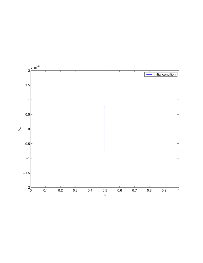
Figure 1: Electron velocity of a square electron acoustic square pulse at time $t=0$

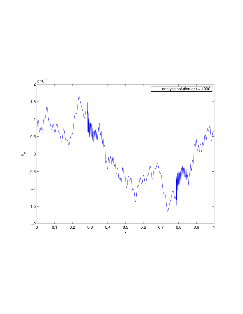
Figure 2: Analytic solution of the electron velocity of a square electron acoustic pulse at time $t=1000$. This plot illustrates the dispersive, non-diffusive nature of the two-fluid system that makes it numerically difficult even in the linear regime. The high frequency modes still contribute significantly to the amplitude of the solution late in time and they always will because there is no physical diffusion. The dispersive, non-diffusive nature of the two-fluid system can make it appear that our numerical solutions suffer from significant numerical dispersion errors when they are actually correctly capturing dispersion described by the model.

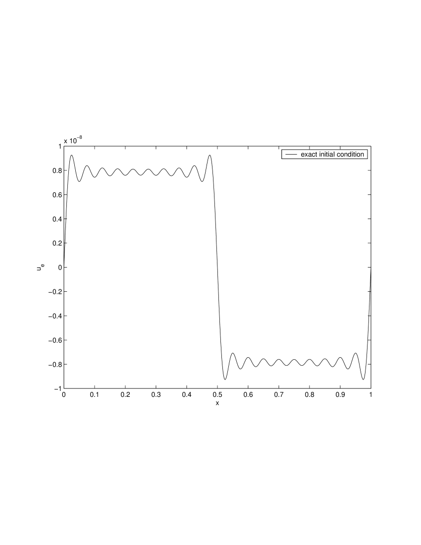
Figure 3: Exact electron x velocity at t=0. Initial conditions are chosen so that all waves travel to the left as time increases. Since the waves are dispersive the initial “square wave” disappears when the solution is allowed to evolve.

After $3$ time units the square pulse shape has disappeared due to wave dispersion. Plots of the numerical solution verses the analytic solution at various grid resolutions are shown in figures 4, 5, and 6 at $3$ time units. In figure 4 there are $40$ cells in the domain and the 3rd order method shows evidence of resolving the highest order mode. The 2nd order method only captures the bulk features.

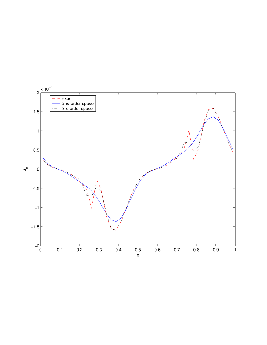
Figure 4: Numerical solution using 2nd and 3rd order discontinuous Galerkin spatial discretizations with a 3rd order time discretization compared to the exact solution at t=3. The grid has $40$ cells so the highest wave number mode is barely resolved with the 2nd order method. The 2nd and 3rd order solutions differ substantially from the analytic solution.

In figure 5 there are $80$ cells in the domain and the 3rd order method captures the amplitude of the highest modes and matches the analytic solution very well. The 2nd order method still struggles to resolve the highest mode (note the solution at the two skinniest spikes).

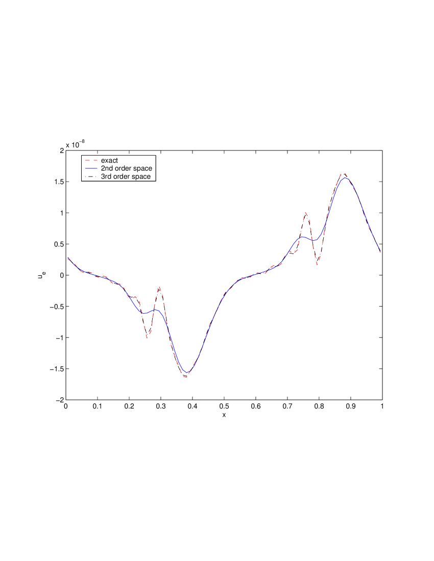
Figure 5: Numerical solution using 2nd and 3rd order discontinuous Galerkin spatial discretizations with a 3rd order time discretization compared to the exact solution at t=3. The grid has $80$ cells across the domain. The 2nd order solution differs substantially from the analytic solution, only capturing the lower order modes. The 3rd order solution matches the analytic solution well.

In figure 6 there are $160$ cells in the domain and the 2nd order method still does not match the amplitude of the highest order mode and does not match the amplitudes much better than the 3rd order method at $40$ grid cells.

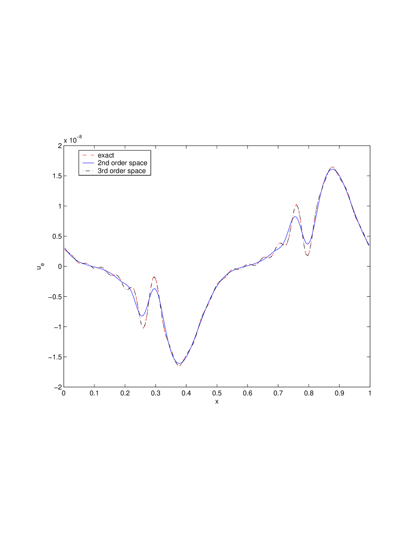
Figure 6: Numerical solution using 2nd and 3rd order discontinuous Galerkin spatial discretizations with a 3rd order time discretization compared to the exact solution at t=3. The grid has $160$ cells across the domain. The 2nd order solution resolves the high order modes at this resolution. At higher resolution the numerical solutions are visually indistinguishable from the analytic solution.

Figure 7 shows a plot of the convergence history of the numerical solutions along with calculated order of accuracy. In both cases the calculated order of accuracy varies from less than $1$ for low resolution where the high frequency modes are barely resolved to better than the order of the scheme when the solution is nearly converged.

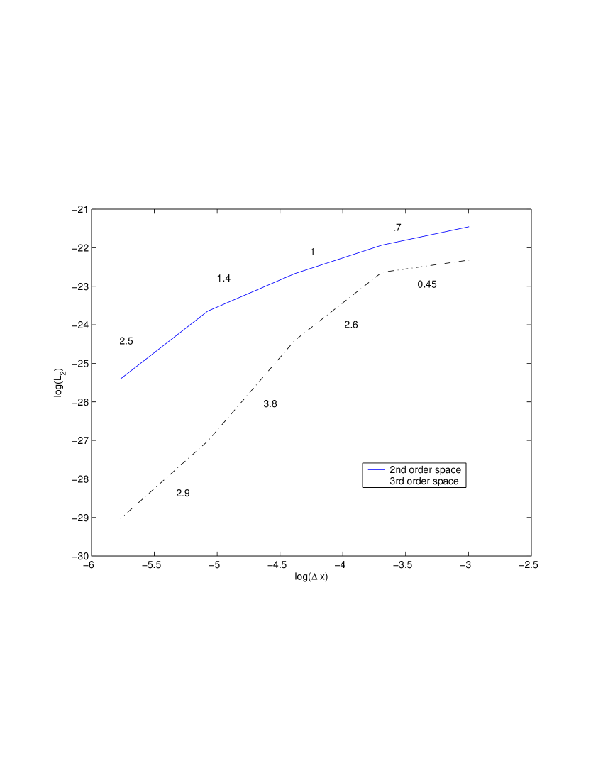
Figure 7: Natural log of the $L_{2}$ norm verses natural log of grid spacing for the numerical solutions to the electron acoustic wave dispersion problem. The solutions were calculated using 2nd and 3rd order discontinuous Galerkin spatial discretizations with a 3rd order Runge-Kutta time discretization. The numbers near each line give the slope of the line and hence the measured order of accuracy of the scheme. The 3rd order method gives substantially better accuracy than the second order method. Grid resolutions used to construct this plot are $1/20$, $1/40$, $1/80$, $1/160$, and $1/320$. The measured accuracy was computed at $t=3$.

The 3rd order method performs substantially better than the 2nd order in this linearized problem when limiter are not needed. In particular, the 3rd order method preserves amplitude much better than the 2nd order, this same phenomena has been observed in certain equilibrium type non-linear problems.

5.1 Two-Fluid Electromagnetic Plasma Shock

The two-fluid electromagnetic plasma shock is an extension of the Brio and Wu shock [45] to the two-fluid plasma model. The simulation was first performed in [1, 46] and is used in the current paper as a benchmark. The ideal two-fluid system has no dissipative terms however an artificial viscosity exists due to the numerical discretization. Wave steepening of the two-fluid solution is limited by physical wave dispersion, when wave dispersion is not sufficient to limit the steepening, artificial viscosity limits the steepening. In real collisionless shocks in experiments and in space, kinetic effects limit the wave steepening when dispersion is not sufficient to limit the steepening. This simulation is meaningful since it illustrates the range of physics that the two-fluid system describes.

In this paper the shock will be presented differently than in [1]. The initial discontinuity is allowed to evolve in time until the shock structure spans $1000r_{g\,i}$ where $r_{g\,i}$ is the ion Larmor radius. Time is measured in terms of light transit times across the entire domain, $\tau_{c}=\frac{1000r_{g\,i}}{c}$. Snapshots of the shock earlier in time correspond to larger characteristic ion Larmor radius, $\frac{r_{g\,i}}{L}<1000$ where $L$ is the span of the shock, and so the solution evolves from a “gas dynamic” regime of short time scales and large characteristic ion Larmor radius $\frac{r_{g\,i}}{L}\gg 1$ to an “MHD” regime of long time scales and small characteristic Larmor radii $\frac{r_{g\,i}}{L}\ll 1$. Parameters used are, $q_{i}=10$, $q_{e}=-10$, and $\epsilon_{0}=1$, $\mu_{0}=1$, $c=1$, $\gamma_{e}=\gamma_{i}=\frac{5}{3}$, $m_{i}=1$, $m_{e}=\frac{1}{1836}$. The initial conditions on the left half of the domain are given by,

$$\left(\begin{array}[]{c}n_{e}\\ U_{e\,x}\\ U_{e\,y}\\ U_{e\,z}\\ P_{e}\\ n_{i}\\ U_{i\,x}\\ U_{i\,y}\\ U_{i\,z}\\ P_{i}\\ B_{x}\\ B_{y}\\ B_{z}\\ E_{x}\\ E_{y}\\ E_{z}\\ \end{array}\right)_{left}=\left(\begin{array}[]{c}1.0\\ 0\\ 0\\ 0\\ 0.5\times 10^{-4}\\ 1.0\\ 0\\ 0\\ 0\\ 0.5\times 10^{-4}\\ 0.75\times 10^{-2}\\ 1.0\times 10^{-2}\\ 0\\ 0\\ 0\\ 0\\ \end{array}\right),\quad\text{and}\quad\left(\begin{array}[]{c}n_{e}\\ U_{e\,x}\\ U_{e\,y}\\ U_{e\,z}\\ P_{e}\\ n_{i}\\ U_{i\,x}\\ U_{i\,y}\\ U_{i\,z}\\ P_{i}\\ B_{x}\\ B_{y}\\ B_{z}\\ E_{x}\\ E_{y}\\ E_{z}\\ \end{array}\right)_{right}=\left(\begin{array}[]{c}0.125\\ 0\\ 0\\ 0\\ 0.05\times 10^{-4}\\ 0.125\\ 0\\ 0\\ 0\\ 0.05\times 10^{-4}\\ 0.75\times 10^{-2}\\ 1.0\times 10^{-2}\\ 0\\ 0\\ 0\\ 0\\ \end{array}\right)\,.$$ (45)

The spatial units of figures 8, 9, 10, 11, 12, 13 are measured in ion Larmor radii $r_{g\,i}$ based on the initial conditions in the left half of the domain. The Debye length is $\lambda_{d}=\frac{1}{100}\,r_{g\,i}$ also based on the initial conditions on the left half of the domain. The results in figure 8 correspond to a less accurate solution to that published in [1] figure 8. The domain of figure 8 has only 500 cells in the domain corresponding to 1000 degrees of freedom (5,000 time steps to reach this point in the simulation) while the published solution using a finite volume method has 4000 cells or 4000 degrees of freedom. In figure 10 the solution is higher resolution than the corresponding solution published in figure 9 of [1] as can be seen by the resolution of the oscillations to the left of the rarefaction wave. At this scale there are 5000 cells in the domain corresponding to 10,000 degrees of freedom (50,000 time steps to reach this point in the simulation) while there are 4000 degrees of freedom in the previously published solution. At the final time figure 12, the solution has moved beyond those published and significant oscillations to the left of the shock are observed. Most of these waves are resolved in several hundred grid cells, and the entire domain of figure 12 is 50,000 cells (500,000 time steps to reach this point in the simulation).

Due to the dispersive, non-diffusive nature of the system, the shocks solutions show more complexity as resolution is increased in time and space. To illustrate this figures 9, 11, 13 show solutions using a time step based $\Delta t=1/\omega_{p\,e}$ compared to the solution with $\Delta t=1/(2\omega_{p\,e})$. These results show the large amount of damping in the $\Delta t=1/\omega_{p\,e}$ case that results from temporally unresolved simulations, however, many of the essential features of the solution still remain. Similarly, increasing the spatial resolution adds higher frequency dispersive waves without significantly changing the overall shape. The final solution 12 took roughly two days on 64 processors so higher resolution solutions were not attempted.

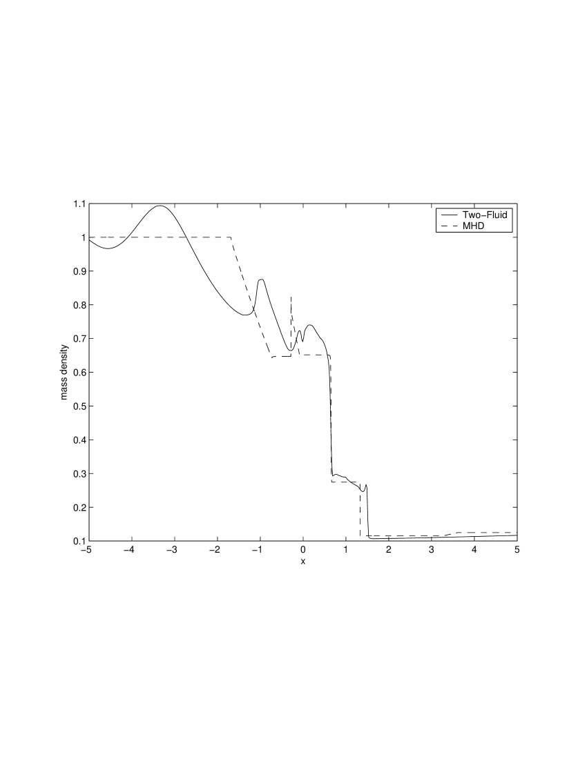
Figure 8: Electromagnetic shock solution using the two-fluid equations and the MHD equations at $t=0.01\tau_{c}$. At this time the domain spans $10$ ion Larmor radii or $1000$ Debye lengths. It is in this regime that the two-fluid solution differs most significantly from the MHD or the “gas dynamic” solution. This regime has practical applications to Z-Pinches and FRC’s due to the weak magnetization of the ions.

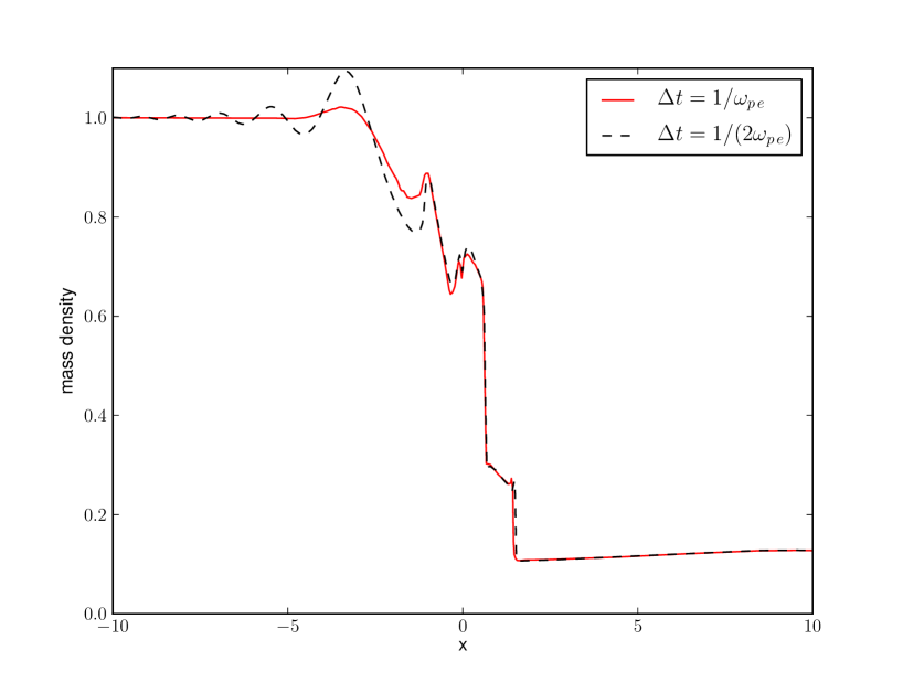
Figure 9: Comparison of $10$ ion Larmor radius solution when the plasma frequency is just resolved compared to a solution with half the time step. Time step close to the stability limit significantly damps the high frequency waves virtually eliminating the trailing wave train.

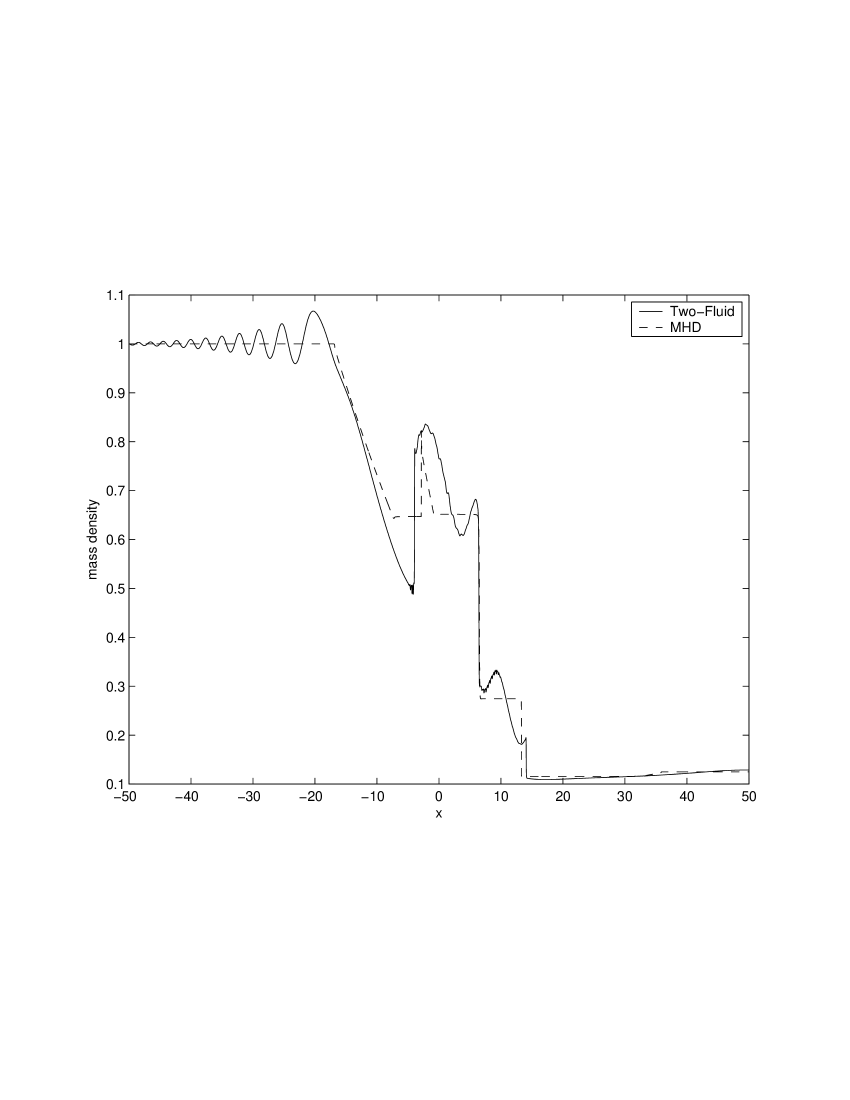
Figure 10: Electromagnetic shock solution using the two-fluid equations and the MHD equations at $t=0.1\tau_{c}$. At this time the domain spans $100$ ion Larmor radii or $10000$ Debye lengths. Major differences from previously published results (Figure 9 in [1] include the large oscillations to the left of the rarefaction wave which are dispersive plasma waves. The differences are a result of the higher grid resolution and better accuracy of the algorithm used in this paper.

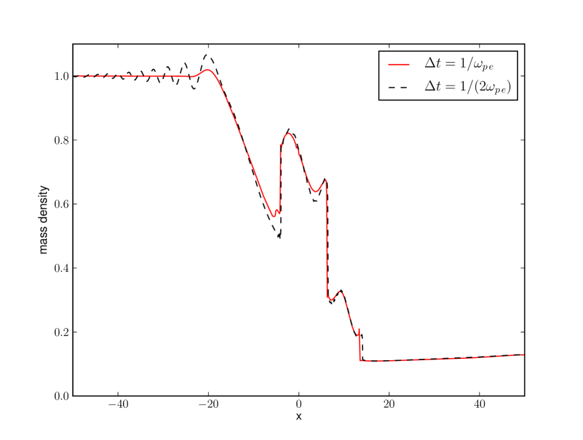
Figure 11: Comparison of $100$ ion Larmor radius solution when the plasma frequency is just resolved compared to a solution with half the time step.

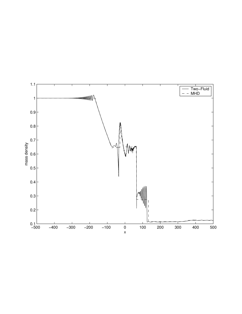
Figure 12: Electromagnetic shock solution using the two-fluid equations and the MHD equations at $t=1\tau_{c}$. At this point in the simulation the solution is very MHD like. However, key differences remain as a result of the fact that the two-fluid system models dispersive MHD waves. The most major differences are the post shock and post rarefaction wave oscillations. Both look numerical, but these waves are resolved in several hundred grid cells and are a result of dispersive plasma waves described in the model. Moving from lower resolution to higher resolution runs show more high frequency waves with less diffusion. This simulations was the highest resolution performed using 50,000 cells. In this regime the Hall MHD model should be used since if one uses the full two-fluid model one needs to approximately resolve the Debye length scales to get good shock solutions. The desire to resolve the Debye length in this simulation means that extremely high resolution was used.

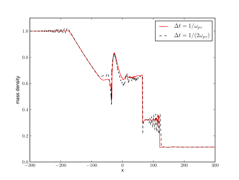
Figure 13: Comparison of $1000$ ion Larmor radius solution when the plasma frequency is just resolved compared to a solution with half the time step. It’s very important to resolve he plasma frequency in order to get the full dynamics of this simulation.

5.2 Magnetic Reconnection

In ideal MHD the fluid is frozen to the magnetic field lines and this prevents one field line from connecting with another. The addition of non-ideal terms such as resistivity results in fluid moving across field lines allowing magnetic reconnection to occur. Classical resistivity leads to much slower reconnection rates than are observed in collisionless space and fusion plasmas. Non-ideal, collisionless terms such as electron inertia and the electron pressure gradient are partially responsible for the fast reconnection that is observed to occur in the earths magnetotail and fusion plasmas. In this section we show that the two-fluid algorithm developed in this paper produces magnetic reconnection rates that agree with those described of the GEM challenge magnetic reconnection problem as described in [2].

The GEM challenge magnetic reconnection problem is non-dimensionalized as in [2] where lengths are normalized by the ion inertial length $d=c/w_{p\,i}=c\,\left(\frac{e^{2}\,n_{0}}{\epsilon_{0}\,m_{i}}\right)^{-\frac{1}{2}}$ time is non-dimensionalized by the ion-cyclotron time $\frac{m_{i}}{e\,B_{0}}$ where $B_{0}$ is the magnetic field at infinity. The velocities are normalized by the Alfven velocity $V_{a}=\left(\frac{B_{0}^{2}}{\mu_{0}\,m_{i}\,n_{0}}\right)^{\frac{1}{2}}$. Finally current density is non-dimensionalized by $J_{0}=\frac{B_{0}\,w_{p\,i}}{\mu_{0}\,c}$ and E by $E_{0}=V_{a}\,B_{0}$. The domain is $\left(-6.4\,d,6.4\,d\right)$ and the simulation is run out to $40/w_{c\,i}$. Conducting walls are used on the $y$ boundaries and periodic boundaries are used on the $x$ boundaries. $\lambda=0.5\,d$, the ion to electron mass ratio is taken to be $25$ and the specific heat ratio $\gamma=\frac{5}{3}$. The speed of light is $c=10\,V_{a}$. The reconnection rates do not change noticeably when the ratio of the speed of light to the Alfven speed is increased to $c=100\,V_{a}$ as was done in [47]. The initial number densities are given by,

$$n_{e}=n_{i}=n_{0}\left(\frac{1}{5}+\text{sech}^{2}\left(\frac{y}{\lambda}\right)\right)\,.$$ (46)

The electron and ion temperatures differ slightly, but are constant throughout the domain, this gives the following electron pressure, $P_{e}$,

$$P_{e}=\frac{1}{12\mu_{0}}B_{0}^{2}\,\frac{n_{e}}{n_{0}}$$ (47)

and ion pressure $P_{i}$

$$P_{i}=\frac{5}{12\mu_{0}}B_{0}^{2}\,\frac{n_{i}}{n_{0}}.$$ (48)

The electron and ion pressure balance the magnetic field which is given by

$$B_{x}=B_{0}\,\text{tanh}\left(\frac{y}{\lambda}\right)+\frac{B_{0}}{10}\frac{\pi}{L_{x}}\cos\left(\frac{2\pi\,x}{L_{x}}\right)\sin\left(\frac{\pi\,y}{L_{y}}\right)$$ (49)

$$B_{y}=\frac{B_{0}}{10}\left(\frac{2\pi}{L_{x}}\right)\sin\left(\frac{2\pi\,x}{L_{x}}\right)\cos\left(\frac{\pi\,y}{L_{y}}\right)$$ (50)

The magnetic field is in equilibrium with with the electron current $J_{z\,e}$,

$$J_{z\,e}=\frac{\mu_{0}\,B_{0}}{\lambda}\,\text{sech}^{2}\left(\frac{x}{\lambda}\right)\,.$$ (51)

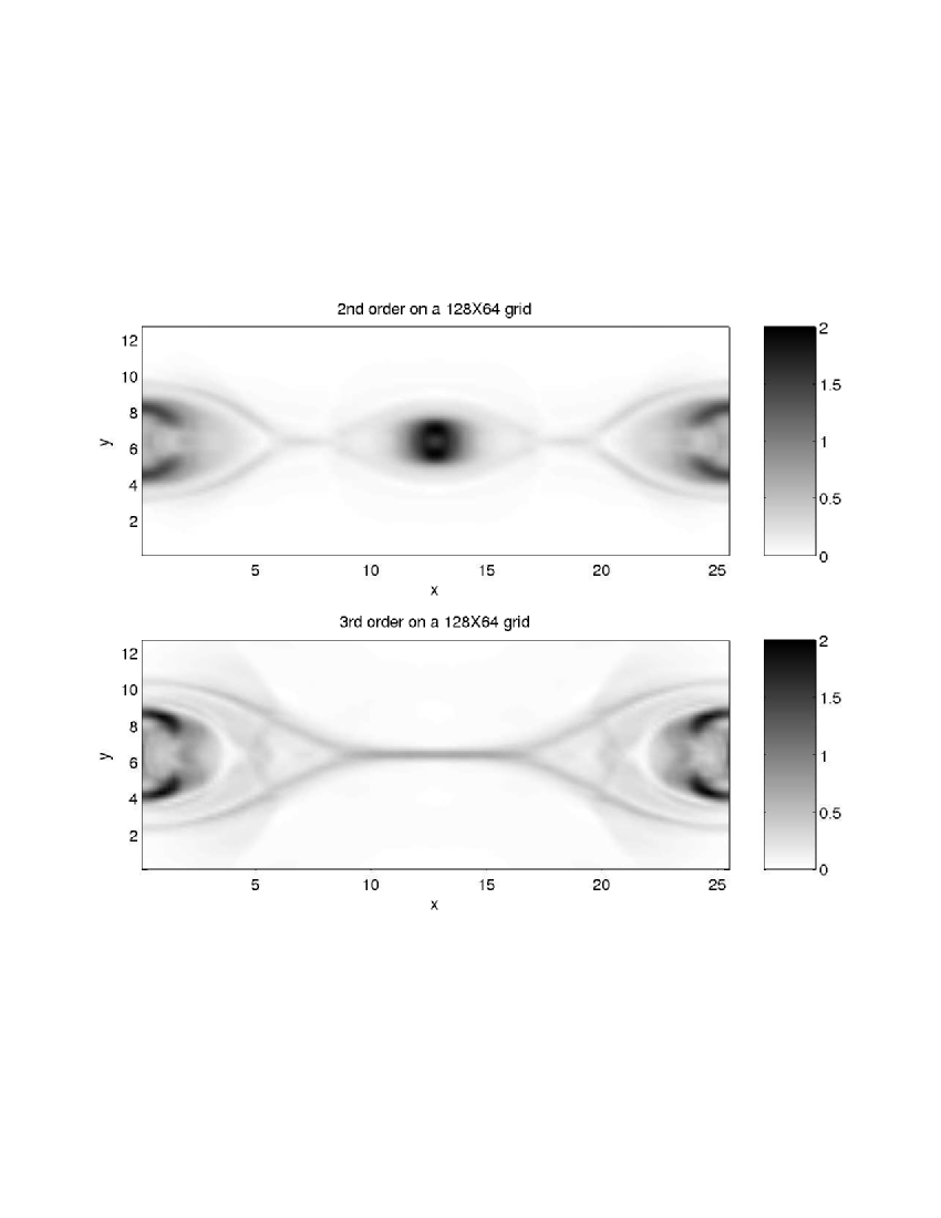
Figure 14: GEM challenge comparing $|J_{z}|$ using the 2nd and 3rd order method on a $128\times 64$ grid at time $t=25/w_{c\,i}$. At this resolution an island forms in the 2nd order method and grows as the simulation progresses. Both methods use 3rd order TVD Runge-Kutta time stepping.

Figure 15: GEM challenge comparing $|J_{z}|$ using the 2nd and 3rd order method on a $512\times 256$ grid at time $t=25/w_{c\,i}$. At this resolution the 2nd and 3rd order method look similar. Both methods use 3rd order TVD Runge-Kutta time stepping. Instabilities develop out of the fluid jets that emerge from the x-point when they collide with the slow moving fluids in the lobes.

The simulations are run at two resolutions, $128\times 64$ and $512\times 256$ using a second or third order discontinuous Galerkin method with third order TVD Runge Kutta time stepping. At a resolution of $512\times 256$, 80 thousand time steps are taken and at a resolution of $128\times 64$, 20 thousand time steps are taken. In figure 14 low resolution solutions to the GEM challenge problem are plotted at $t=25/\omega_{c\,i}$. The second order solution shows stable island formation while in the third order method no island forms. In this simulation the TVB limiter constant $M=0$ is used to eliminate the formation of an unstable island in the third order method. Solutions to the GEM challenge problem are highly susceptible to bifurcation [48] which is the formation of magnetic islands at or near the x-point (the center of the domain in this case). The development of these islands may be due to excessive dissipation applied at the x-point; however, the development of islands can be unpredictable and in the case of the 3rd order method, increased dissipation can actually eliminate the island.

The islands are unstable and any small perturbation in the location or fields in the island will cause the island to slip and merge with one of the lobes. Small perturbations can arise from machine precision error and this is particularly true at locations near equilibrium where two nearly equal but opposing forces are added, the number that remains may depend significantly on the precision of the numbers used. It has been observed that increasing machine precision can change the direction that an unstable island slips off to. The second order solution shows the formation of a stable island presumably due to the extra dissipation of the second order method.

In figure 15 the high resolution solutions are plotted at $t=25/\omega_{c\,i}$ with the TVB limiter constant $M=25$. At this resolution the second and third order methods produce very similar results. In this case no island formation is visible in either the second or third order schemes, however at time $t=30/\omega_{c\,i}$ a very small unstable island forms in the 3rd order method and combines with the left lobe before $t=35/\omega_{c\,i}$.

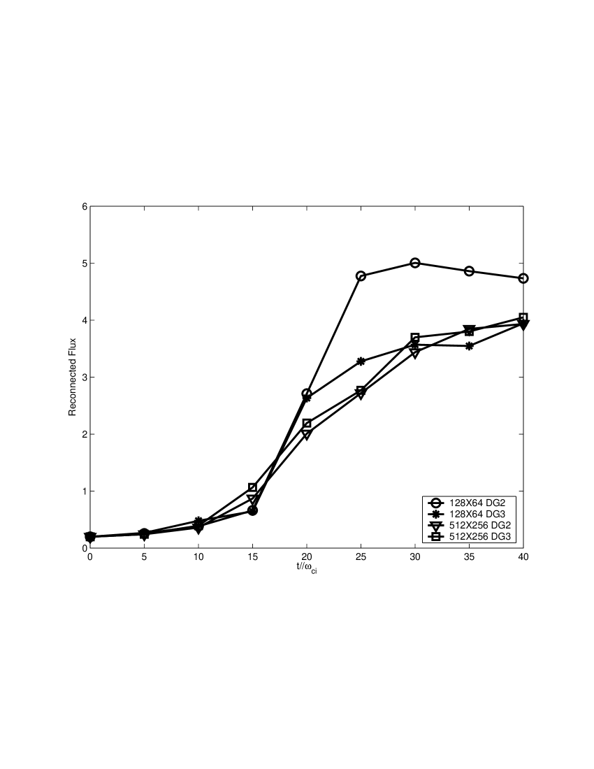
Figure 16: Plot of reconnected flux vs time for 2nd and 3rd order spatial discretizations at resolutions of $128\times 64$ and $512\times 256$. The reconnected flux differs substantially for the two methods at $128\times 64$, though the 3rd order method better matches the high order solutions. At $512\times 128$ the 2nd and 3rd order methods are in close agreement.

In figure 16 the reconnected magnetic flux $\frac{1}{2}\int|B_{y}|dx$ along the x axis is plotted for several solutions. At grid resolution of $512\times 256$ the second and third order methods produce similar results. At a resolution of $128\times 64$ the third order method produces results which are in much better agreement with the high resolution results than does the second order method.

In figure 17 the reconnected flux up to time $t=60/\omega_{c\,i}$ is shown illustrating the saturation of the numerical solution beyond the published time interval in the GEM challenge results [2].

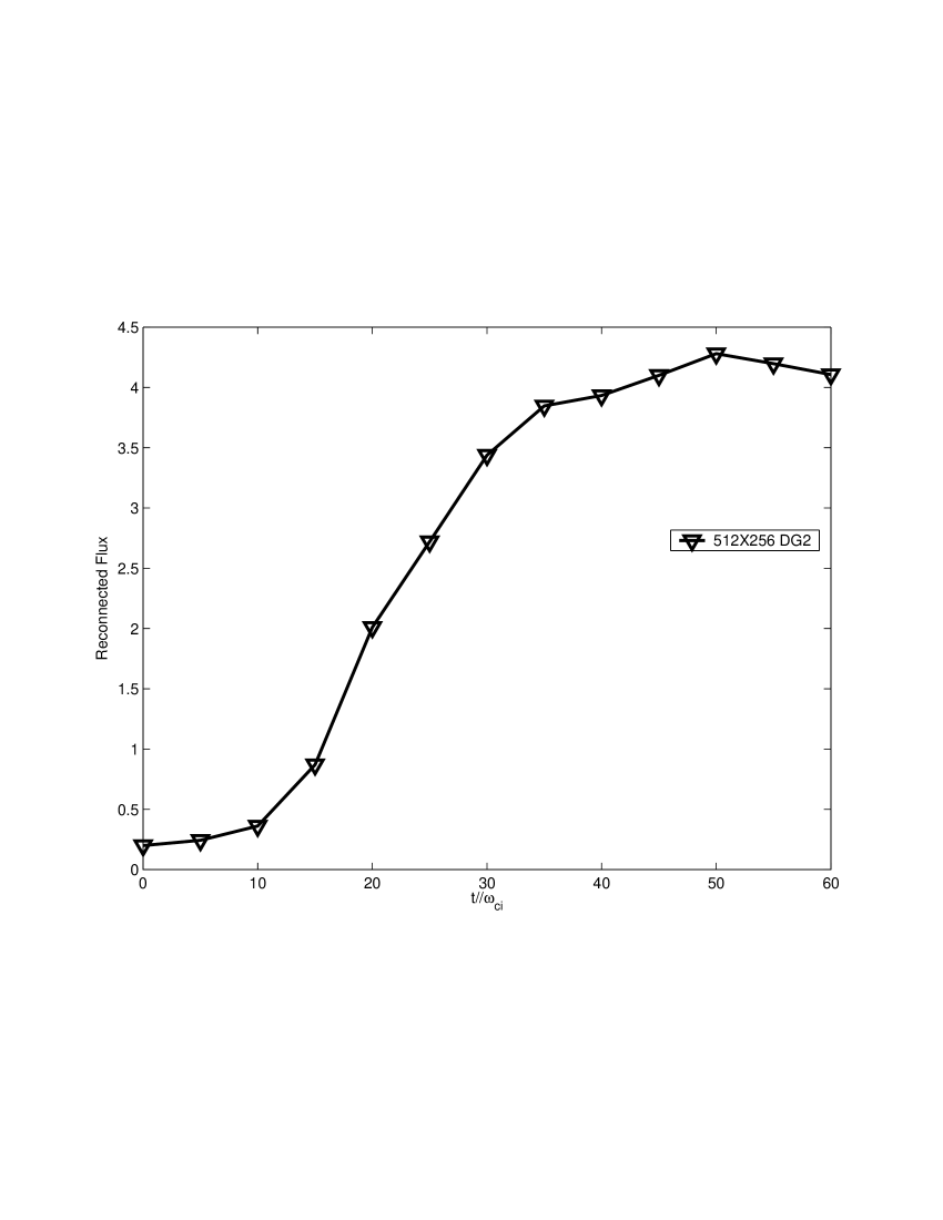
Figure 17: Plot of reconnected magnetic flux to time $t=60/\omega_{c\,i}$ for a $512X256$ solution. This figure shows that the two-fluid solution does saturate as would be expected with conducting walls and finite flux in the domain.

Flows appear late in time which are turbulent as shown in figure 18 at time $t=40/\omega_{c\,i}$. The 3rd order method shows considerably more asymmetry than the 2nd order method, but asymmetry has begun to develop in the 2nd order solution. This asymmetry develops out of machine precision errors that are initiated in the current layer at the x-point from the balancing of source terms and fluxes. The only dissipation present is numerical so the second order method tends smooth out the errors produced by the finite precision more than the 3rd order method. As a result of the low dissipation in the 3rd order method these errors result in the excitation of unstable modes which eventually effect the macroscopic solution. The magnitude of electron momentum can differ by as much as 10 percent by moving from 64 bit numbers to 80 bit numbers at $t=40/\omega_{c\,i}$; fortunately these regions tend to be localized.

Notice the pair of shocks in figure 18, the positions differ in the two solutions. The positions differ because the onset of the fast growth stage is slightly different for the two methods. As the fast growth begins, shocks form in the ion fluid as it is accelerated along the $x$ axis. Eventually the two jets of shocked ion fluid collided and two shock that spans the $y$ axis are formed which continues to propagate through the domain as the solution evolves. If the onset of fast growth differs slightly initially, then these shocks will appear at different locations for a given time.

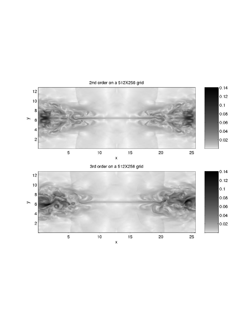
Figure 18: Plot of total ion momentum at $t=40/\omega_{c\,i}$ at a resolution of $512\times 256$ using the second and third order DG methods.

6 Discussion

A discontinuous Galerkin method for the ideal 5-moment two-fluid plasma system is developed. A scalar model problem of the ideal two-fluid system is derived to illustrate the character of the full system. An analytic two-fluid solution to an electron acoustic square pulse in the linear regime is derived and the numerical solution using the fully non-linear two-fluid system is calculated showing convergence for the 2nd and 3rd order discontinuous Galerkin methods. The algorithm is benchmarked against the two-fluid electromagnetic shock originally published in [1]. The 2nd and 3rd order algorithms are tested on the GEM challenge magnetic reconnection problem and produces results comparable to those generated by particle codes, hybrid codes, and a Hall MHD code in [49]. The discontinuous Galerkin method offers a straight forward method for solving the ideal 5-moment two-fluid system. This same algorithm could be applied to 10 and higher moment two-fluid systems. The algorithm can be easily generalized to three dimensions and general geometries.

References

- [1] U. Shumlak, J. Loverich, Approximate riemann solver for the two-fluid plasma model, Journal of Computational Physics 187 (2003) 620–638.
- [2] J. Birn, et al., Geospace environmental modeling (gem) magnetic reconnection challenge, Journal of Geophysical Research 106 (A3) (2001) 3715–3719.
- [3] J. P. Freidberg, Ideal Magnetohydrodynamics, Plenum Press, 1987.
- [4] P. M. Bellan, Spheromaks, Imperial College Press, 2000.
- [5] A. Hakim, U. Shumlak, Two-fluid physics and field-reversed configurations, Physics of Plasmas 14 (5) (2007) 055911.
- [6] J. W. Connor, Pressure gradient turbulent transport and collisionless reconnection, Plasma Physics and Controlled Fusions 35 (1993) 757–763.
- [7] N. A. Krall, P. C. Liewer, Low-frequency instabilities in magnetic pulses, Physical Review A 4 (5) (1971) 2094–2103.
- [8] R. C. Davidson, N. T. Gladd, Anomalous transport properties associated with the lower-hybrid-drift instability, The Physics of Fluids 18 (10) (1975) 1327–1335.
- [9] J. Loverich, U. Shumlak, Nonlinear full two-fluid study of m = 0 sausage instabilities in an axisymmetric z pinch, Physics of Plasmas 13 (8) (2006) 082310.
- [10] L. Solovev, Dynamics of a cylindrical z pinch, Soviet Journal of Plasma Physics 10 (5) (1984) 602–605.
- [11] M. Haines, The physics of the dense z-pinch in theory and in experiment with application to fusion reactor, Physica Scripta T2/2 (1982) 380–390.
- [12] O. S. Jones, U. Shumlak, D. S. Eberhardt, An implicit scheme for nonideal magnetohydrodynamics, Journal Of Computational Physics 130 (1997) 231–242.
- [13] C. Sovinec, et al., Nonlinear magnetohydrodynamics simulation using high-order finite elements, Journal of Computational Physics 195 (2004) 355–386.
- [14] A. Bhattacharjee, Center for magnetic reconnection studies: Present status, future plans, PSACI PAC Presentation, Princeton (June 2003).
- [15] J. Breslau, S. Jardin, A parallel algorithm for global magnetic reconnection studies, Computer Physics Communications 151 (2003) 8–24.
- [16] J. D. Huba, Hall magnetohydrodynamics - a tutorial, in: M. S. J. Buchner, C.T. Dunn (Ed.), Space Plasma Simulation, Springer, 2003, pp. 166–192.
- [17] W. Park, et al., Plasma simulation studies using multilevel physics models, Physics of Plasmas 6 (5) (1999) 1796–1803.
- [18] S. Baboolal, Finite-difference modeling of solitons induced by a density hump in a plasma multi-fluid, Mathematics and Computers in Simulation 55 (2001) 309–316.
- [19] R. Schneider, C. D. Munz, The approximation of two-fluid plasma flow with explicit upwind schemes, International Journal of Numerical Modelling: Electronic Networks, Devices and Fields 8 (1995) 399–416.
- [20] P. Rambo, J. Denavit, Time-implicit fluid simulation of collisional plasmas, Journal Of Computational Physics 98 (1991) 317–331.
- [21] R. Mason, An electromagnetic field algorithm for 2d implicit plasma simulation, Journal of Computational Physics 71 (1987) 429–473.
- [22] R. Mason, C. Cranfill, Hybrid two-dimensional electron transport in self-consistent electromagnetic fields, IEEE Transactions on Plasma Science 14 (1) (1986) 45–52.
- [23] A. Hakim, J. Loverich, U. Shumlak, A high resolution wave propagation scheme for ideal two-fluid plasma equations, J. Comput. Phys. 219 (1) (2006) 418–442.
- [24] B. Cockburn, C.-W. Shu, Tvb runge-kutta local projection discontinuous galerkin finite element method for conservation laws ii: General framework, Mathematics of Computation 52 (1989) 411–435.
- [25] B. Cockburn, S.-Y. Lin, C.-W. Shu, Tvb runge-kutta local projection discontinuous galerkin finite element method for conservation laws iii: One-dimensional systems, Journal of Computational Physics 84 (1989) 90–113.
- [26] B. Cockburn, S. Hou, C.-W. Shu, The runge-kutta local projection discontinuous galerkin finite element method for conservation laws iv: Multidimensional case, Mathematics of Computation 54 (1990) 545–581.
- [27] B. Cockburn, C.-W. Shu, The runge-kutta discontinuous galerkin method for conservation laws v: Multidimensional systems, Journal of Computational Physics 141 (1998) 199–224.
- [28] J. S. Hesthaven, T. Warburton, Nodal high-order methods on unstructured grids, Journal of Computational Physics 181 (2002) 186–221.
- [29] B. Cockburn, F. Li, C.-W. Shu, Locally divergence-free discontinuous galerkin methods for maxwell’s equations, Journal of Computational Physics 194 (2004) 588–610.
- [30] T. C. Warburton, G. E. Karniadakis, A discontinuous galerkin method for the viscous mhd equations, Journal of Computational Physics 152 (1999) 608–641.
- [31] G. Lin, G. Karniadakis, A discontinuous galerkin method for two-temperature plasmas, Comput. Methods Appl. Mech. Engrg. 195 (2006) 3504–3527.
- [32] A. Mangeney, F. Califano, C. Cavazzoni, P. Travnicek, A numerical scheme for the integration of the vlasov-maxwell system of equations, Journal of Computational Physics 179 (2002) 495–538.
- [33] B. Cockburn, G. E. Karniadakis, C.-W. Shu (Eds.), Discontinuous Galerkin Methods, Springer, 2000.
- [34] C. D. Munz, R. Schneider, U. Vos, A finite-volume method for the maxwell equations in the time domain, Siam Journal of Scientific Computing 22 (2000) 449–475.
- [35] T. Umeda, Y. Omura, T. Tominaga, H. Matsumoto, A new charge conservation method in electromagnetic particle-in-cell simulations, Computer Physics Communications 156 (2003) 73–85.
- [36] J. Villasenor, O. Buneman, Rigorous charge conservation for local electromagnetic field solvers, Computer Physics Communications 69 (2-3) (1992) 306–316.
- [37] P. J. Mardahl, J. P. Verboncoeur, Charge conservation in electromagnetic PIC codes; spectral comparison of Boris/DADI and Langdon-Marder methods, Computer Physics Communications 106 (1997) 219–229.
- [38] S. Li, High order central scheme on overlapping cells for magneto-hydrodynamic flows with and without constrained transport method, J. Comput. Phys. 227 (15) (2008) 7368–7393.
- [39] D. S. Balsara, Divergence-free reconstruction of magnetic fields and weno schemes for magnetohydrodynamics, J. Comput. Phys. 228 (14) (2009) 5040–5056.
- [40] T. A. Gardiner, J. M. Stone, An unsplit godunov method for ideal mhd via constrained transport in three dimensions, J. Comput. Phys. 227 (8) (2008) 4123–4141.
- [41] P. Londrillo, L. D. Zanna, On the divergence-free condition in godunov-type schemes for ideal magnetohydrodynamics: the upwind constrained transport method, J. Comput. Phys. 195 (1) (2004) 17–48.
- [42] D. Durran, Numerical Methods for Wave Equations in Geophysical Fluid Dynamics, Springer, 1998.
- [43] R. J. LeVeque, Finite Volume Methods for Hyperbolic Problems, Cambridge University Press, 2002.
- [44] R. Biswas, K. D. Devine, J. E. Flaherty, Parallel, adaptive finite element methods for conservation laws, Applied Numerical Mathematics 14 (1994) 255–283.
- [45] M. Brio, C. C. Wu, An upwind differencing scheme for the equations of ideal magnetohydrodynamics, Journal Of Computational Physics 75 (1988) 400–422.
- [46] J. Loverich, A finite volume algorithm for the two-fluid plasma system in one dimension, Masters thesis, University of Washington (2003).
- [47] J. Loverich, U. Shumlak, A discontinuous galerkin method for the full two-fluid plasma model, Computer Physics Communications 169 (2005) 251–255.
- [48] M. Hesse, J. Birn, M. Kusnetsova, Collisionless magnetic reconnection: Electron processes and transport modeling, Journal of Geophysical Research 106 (2001) 3721–3735.
- [49] M. A. Shay, J. F. Drake, B. N. Rogers, R. E. Denton, Alfvenic collisionless magnetic reconnection and the hall term, Journal of Geophysical Research 106 (2001) 3759–3772.