UCAC3 pixel processing

Abstract

The third US Naval Observatory (USNO) CCD Astrograph Catalog, UCAC3 was released at the IAU General Assembly on 2009 August 10. It is a highly accurate, all-sky astrometric catalog of about 100 million stars in the R = 8 to 16 magnitude range. Recent epoch observations are based on over 270,000 CCD exposures, which have been re-processed for the UCAC3 release applying traditional and new techniques. Challenges in the data have been high dark current and asymmetric image profiles due to the poor charge transfer efficiency of the detector. Non-Gaussian image profile functions were explored and correlations are found for profile fit parameters with properties of the CCD frames. These were utilized to constrain the image profile fit models and adequately describe the observed point-spread function of stellar images with a minimum number of free parameters. Using an appropriate model function, blended images of double stars could be fit successfully. UCAC3 positions are derived from 2-dimensional image profile fits with a 5-parameter, symmetric Lorentz profile model. Internal precisions of about 5 mas per coordinate and single exposure are found, which are degraded by the atmosphere to about 10 mas. However, systematic errors exceeding 100 mas are present in the $x,y$ data which have been corrected in the astrometric reductions following the $x,y$ data reduction step described here.

1 INTRODUCTION

The US Naval Observatory (USNO) operated the 8-inch (0.2 m) Twin Astrograph between 1998 and 2004 for the first ever all-sky astrometric survey using a CCD detector. About 2/3 of the sky was observed from the Cerro Tololo Inter-American Observatory (CTIO) while the rest of the northern sky was observed from the Naval Observatory Flagstaff Station (NOFS). In 1998 the Kodak 4k by 4k CCD detector used for this UCAC project was the largest number of pixels chip at any telescopes at CTIO. The UCAC project also brought attention to a potential source of systematic errors for astrometry using CCDs, the charge-transfer inefficiency.

The first paper describing the UCAC1 release (Zacharias et al., 2000) gives details about the observing procedures and initial reductions. The second release, UCAC2, (Zacharias et al., 2004), is an extension of UCAC1 applying similar reduction methods to a much larger area of the sky. The same pixel processing pipeline was used for UCAC1 and UCAC2, while improved systematic error corrections were introduced for the UCAC2 reductions to obtain celestial coordinates. The UCAC2 is being used extensively by the astronomical community, providing a much needed densification of the optical celestial reference frame at magnitudes fainter than the Hipparcos and Tycho-2 catalogs. The UCAC observations cover mainly the 8 to 16 magnitude range, providing accurate star positions with external errors of about 20 to 70 milliarcsecond (mas) depending on magnitude.

For the recent UCAC3 release (Zacharias et al., 2010) completely new reductions of the pixel data were performed, involving new analysis methods. These reductions and results are described in this paper in detail, including image profile fitting methods leading to $x,y$ centers. The subsequent astrometric processing from $x,y$ data to celestial coordinates is described in a separate paper (Finch, Zacharias & Wycoff, 2010).

Point-spread function (PSF) fitting has been performed in the past, see for example (Anderson & King, 2000) for HST data, or the IRAF DAOPHOT package (Stetson, 1987). The approach taken here is different, deriving relatively simple, analytical model functions which describe the observed PSF sufficiently well. At the same time the number of free parameters needed for each image profile fit is kept to a minimum by utilizing information from many CCD exposures to constrain some image profile model parameters. Challenges here are asymmetric PSFs and variations of the PSFs over the field of view, combined with a relatively small number of stars per CCD frame and the goal of high astrometric accuracy.

2 PIXEL DATA

A 4094 by 4094 pixel CCD with a 9 $\mu$m pixel size was used in a single bandpass (579 to 643 nm) providing a field of view (FOV) of just over 1 square degree, taking advantage of only a tiny fraction of the flat FOV delivered by the optical system of the Twin Astrograph’s “red lens.” This camera provides 14 bit output and has a gain setting of 5.65 electrons (e^-) per analog-to-digital unit (ADU), 13 e^- read noise, and about 85,000 e^- full well capacity.

A 2-fold overlap pattern of 85,158 fields spans the entire sky. Each field was observed with a long (about 125 s) and a short (about 25 s) exposure. The raw pixel data are stored in custom FITS differential compress (fdc) format files, about 16 MB per exposure without loss of the 14 bit dynamic range.

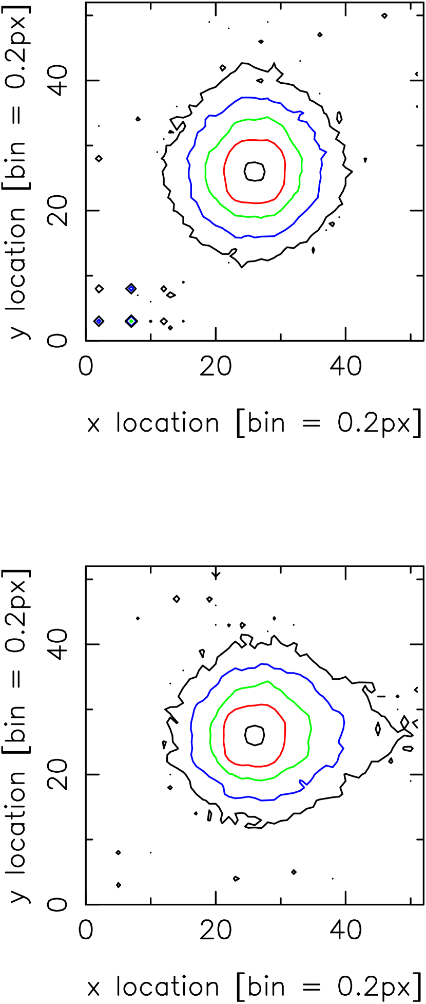
Figure 1: Contour plot of supersampled (see text) images of CCD frame 134473. Average data from near the output register (top) and farther away from it (bottom) are shown. This illustrates the low charge transfer efficiency problem of the detector leading to images which are asymmetric as a function of the $x$ pixel coordinate. The contour levels are at 90%, 30%, 10%, 3% and 1% of the peak intensity.

The detector features a poor charge transfer efficiency (CTE) leading to asymmetric images along the readout direction ($x$ axis) which vary as a function of distance from the output register. This leads to systematic errors in the star positions as a function of $x$ and the stars’ brightness (magnitude), about the worst thing what can happen for an astrometric instrument. The contour plots in Fig. 1 illustrate this problem showing the change of image shape (from almost circular to pronounced asymmetric) as seen on the left and right side of the detector, respectively. The left side (low $x$) is close to the readout register and also displays the largest background noise on the chip, likely due to a higher than average temperature there. Initially the camera showed a “glowing spot” in the lower left corner. The design was changed to have the read amplifier powered up only when needed, which eliminated that problem.

In order to mitigate these $x$ and magnitude dependent systematic errors the detector was operated at a relatively high temperature ($-18C$), which filled many of the CTE causing traps on the silicon detector. Unfortunately the warm operating temperature leads to a substantial dark current. Frequent darks were taken throughout the project for each of the standard exposure times (5, 10, 20, 25, 30, 40, 100, 125, 150, 200 s). Some time into the project it was discovered that the darks also depend on ambient temperature and vacuum pressure inside the camera, which due to small leaks increased from about 0.1 torr to over 2 torr, when a new pumpout of the camera was performed every few months.

3 RAW DATA PROCESSING STEPS

3.1 Combined darks and bad pixel map

The detector used for the UCAC survey has a high cosmetic quality with no bad columns and relatively few bad pixels. In order to simplify the reductions and assuming the worst case, a single list of all possible bad pixels were established spanning dark exposures taken during the entire project.

Early on it was discovered that darks taken during daytime or in rapid succession display different properties than object frames taken during regular observing. Most darks therefore were taken during cloudy nights with a script to obtain about 50 darks of a given integration time in an automated sequence. Pauses of about a minute between dark exposures were introduced to closely resemble actual observing conditions. Using custom software these 50 FITS files were read in parallel, block by block and the 50 measures of each pixel sorted. The mean pixel value was calculated after rejecting about 10 % of the lowest and highest values. This way every few weeks a new combined dark was constructed for every standard exposure time used during that period.

To identify bad pixels comprehensive samples of combined darks of a given exposure time were compared, pixel by pixel. If either the scatter or the mean pixel value exceeded adopted thresholds (about 3-sigma level), that pixel was flagged as “bad”. This process was repeated for all exposure times and a combined list of pixels generated of those pixels which appeared at least once on any of the individual “bad” pixel lists. A total of 13,094 such pixels was identified, which is less than 0.1 % of all pixels on the detector.

3.2 Applying darks

The average background intensity (from bias and dark current) of raw CCD frames taken with our 4k camera is very nonuniform over the field. However, the pattern is very similar from exposure to exposure, while the amplitude of the pattern depends on many things, like exposure time, ambient temperature and vacuum pressure. The mean difference in background ADU between the left and right side of the CCD frame serves as a parameter to quantify the amplitude of this background pattern.

The re-processing of the pixel data was split up into batches of about 10,000 consecutive CCD frames taken over a narrow range of epochs. A pair of appropriate master darks for each standard exposure time was selected. Each pair spans a range in background differences (left to right, see above) that is as large as possible with the restriction of being taken close to the epoch of the frames under investigation. The raw data processing then involved a determination of the mean background difference (left to right) of each individual frame. This value was used in a linear interpolation between the 2 master darks selected for that set of data and the exposure time of the object frame. The pixel-by-pixel interpolated dark was then subtracted from the object frame.

This method of dark subtraction was new for UCAC3 and resulted in a significant improvement in background flatness and lower noise, which leads to a deeper and more uniform limiting magnitude than before. For UCAC2 a more or less random pick of a dark near the target properties was selected without interpolation. As with previous releases, no additional bias frames were needed.

3.3 Flats

Due to the small size of the field utilized by the CCD, as compared to the optical design of the astrograph, there is no vignetting from the optical system expected. Initial tests also revealed only small pixel-to-pixel sensitivity variations. The window on the camera serves as the only filter in a sealed system without moving parts. Thus for the UCAC1 and UCAC2 releases no flats were applied at all to the survey data, aiming at astrometric results without the goal of precise photometry.

However, a set of about 25 dome flats were taken every few months with an exposure time of 5 s and light intensity set to give about 30 to 50% full well capacity illumination. These data were reduced and applied for the UCAC3 release. The appropriate combined dark frame was subtracted from each individual flat exposure, and all flats of a given epoch were combined excluding extreme low and high counts, similarly to the darks processing described above. The flats were scaled to 1000 ADU mean intensity (integer) representing a factor of 1.0 for the science frames data processing to follow. For some epochs the flat data were split into 2 groups of high/low average illumination to check on internal consistency. A total of 28 combined master flats was thus obtained spanning the entire duration of the UCAC observing.

The pixel-to-pixel sensitivity variations are small. Taking 1/25 of the entire CCD area at a time, sorting all the pixels of a given master flat and cutting the low 5% and high 5% of the pixels, the resulting standard deviation for pixel-to-pixel variation is only on the order of 0.4 to 0.6% of the mean pixel count. This fact explains why excellent astrometric results (center fit precision close to 1/100 pixel) were obtained in UCAC2 even without applying any flats.

Large-scale sensitivity variations over the CCD frame area were found to be 10% or less. Comparing different master flats of different epochs, variations of about 2% or less are found, except for the set taken around night numbers 2000 to 2150 (truncated Julian Dates), where significant deviations due to a shutter failure problem are found in the corners of CCD frames.

Based on these results a single master flat file close to the epoch of each object frame was selected and applied. The $\approx$ 10% vignetting in the corners of the CCD frames was attributed to a slightly undersized, round opening of the shutter in our 4k camera system.

4 IMAGE PROFILES

4.1 Supersampling

In order to investigate the shape of the point-spread function (PSF) as seen in the UCAC data the following standard procedure was adopted. Individual CCD frames of good quality taken in areas of the sky with large numbers of stars (but not too crowded, few blended images) were selected. Centers of stellar images were determined by least-square fits using a 2-dimensional Gaussian model of the pixel intensity ($I$) as a function of the pixel coordinates ($x,y$),

$$I(x,y)=B+A\ e^{-\frac{r^{2}ln(2)}{r_{0}^{2}}}$$ (1)

with $r^{2}=(x-x_{0})^{2}+(y-y_{0})^{2}$. We call this model 1 and it has 5 free parameters: the average local background intensity ($B$), the amplitude ($A$), the width of the profile ($r_{0}$), and the image center coordinates $x_{0}$ and $y_{0}$. The natural logarithm of 2 is included here to scale the $r_{0}$ to obtain the radius of the profile at half maximum.

Images with sufficient signal-to-noise (S/N) ratio, but not saturated, were scaled to a fixed amplitude, shifted in $x,y$ pixel coordinates to align centers and resampled onto a grid with 0.2 pixel resolution. Averages of the pixel values in each bin were taken to produce the supersampled PSF representative for that particular CCD frame or sub-area of it. For some of the investigations presented below, a CCD frame was split into 3 equal area sections along the $x$-axis, following increased effects of the poor CTE of the detector. Marginal profiles were calculated from these 2-dim supersampled PSFs along the $x$ and $y$ axis, labeled as $u$ and $v$ coordinates. A 1-dim radial profile was generated for 0.2 pixel bins using the original pixel data and assuming a circular symmetric intensity distribution. The spatial coordinate for those profiles is called $r$, as defined above.

4.2 Profile model functions

An overview of all profile models used for UCAC3 reductions and tests is given in Table 1. Models 1 through 4 are taken from the software for analyzing astrometric CCD data (SAAC) (Winter, 1999), which developed out of earlier work (Schramm, 1998), while the other models have been modified from SAAC models or are newly developed. Model 1 is given by Eq. 1, while model 2 did perform better than model 1 but worse than model 4 and is not further discussed here. Model 4 is the general Lorentz profile function, given as

$$I(x,y)=B\ +\ A\ \left[1+\left(\frac{r}{r_{0}}\right)^{\alpha}\ \left(2^{1/\beta}-1\right)\right]^{-\beta}$$ (2)

For $\beta=1$ this reduces to the Moffat profile (Moffat, 1969). The additional parameter in model 4 gives more control over the shape of the PSF, allowing adjustment of the gradient near the core of the profile independently from the gradient out in the wings.

The profile function of model 4 with a fixed, preset parameter $\beta$ (not determined in the least-squares fit as a free parameter) we call here model 3. Similarly, a function with both parameters $\beta$ and $\alpha$ preset we call model 5.

Derived from the circular, symmetric, Gaussian profile (model 1) an elliptical symmetric function with major and minor axes aligned to $x$ and $y$, respectively (model 6) is defined by

$$I(x,y)=B+A\ e^{-ln(2)\left(\frac{(x-x_{0})^{2}}{a^{2}}+\frac{(y-y_{0})^{2}}{b^{2}}\right)}$$ (3)

where $B$, $A$, $x_{0}$, and $y_{0}$ are defined as before and $a$ and $b$ are the widths of the profile along the $x$ and $y$ axis, respectively.

Model 7 is a generalization of model 6 with the additional free parameter $\theta$ describing the angle of the major axis with the $x$ axis (range $\pm\pi/2$), and is given by

$$I(x,y)=B+A\ e^{-\left((x-x_{0})^{2}c_{x}+(y-y_{0})^{2}c_{y}+(x-x_{0})(y-y_{0})c_{m}\right)}$$ (4)

with

$$c_{x}=\frac{1}{2}\left(\frac{\cos^{2}(\theta)}{a^{2}}+\frac{\sin^{2}(\theta)}{b^{2}}\right)$$

$$c_{y}=\frac{1}{2}\left(\frac{\cos^{2}(\theta)}{b^{2}}+\frac{\sin^{2}(\theta)}{a^{2}}\right)$$

$$c_{m}=-\cos(\theta)\sin(\theta)\left(\frac{1}{b^{2}}-\frac{1}{a^{2}}\right)$$

which reduces to model 6 for $\theta$ = 0.

Tests with asymmetric profiles were performed by adding the following term to each base model ($F$, as given above) in the description of the pixel intensities as function of $x,y$

$$I(x,y)=B+A\ F(r)\ +\ A\ c\ (x-x_{0})\ F(r)$$ (5)

This adds an asymmetric part to the $x$ component with an amplitude factor, $c$. Extending this concept to an additional asymmetric contribution along the $y$ axis is straightforward.

The following model was used for some tests. It is based on a generalized Lorentz profile (elliptical) with asymmetric terms for $x$ and $y$,

$$I(x,y)=B\ +\ A^{\prime}\ \left[1+\left(\frac{r}{r_{0}}\right)^{\alpha}\ \left(2^{1/\beta}-1\right)\right]^{-\beta}$$ (6)

with

$$\Delta x=x-x_{0}$$

$$\Delta y=y-y_{0}$$

$$\frac{r}{r_{0}}=\sqrt{\frac{\Delta x^{2}}{a^{2}}+\frac{\Delta y^{2}}{b^{2}}}$$

$$A^{\prime}=A\left[1+c_{x}\Delta x+c_{y}\Delta y\right]$$

with background $B$, amplitude $A$, image center $x_{0},y_{0}$, profile shape parameters $\alpha,\beta$ as before, and radius of profile width along $x$ and $y$, $a,b$, respectively (elliptical model). The asymmetry in this model is described by the parameters $c_{x}$, and $c_{y}$ for the relative amplitude of the asymmetry along $x$ and $y$, respectively, giving a total of 10 parameters. This profile function was used for models 12 to 14, depending on which of these parameters are preset and which are free fit parameters (see Table 1).

4.3 First results

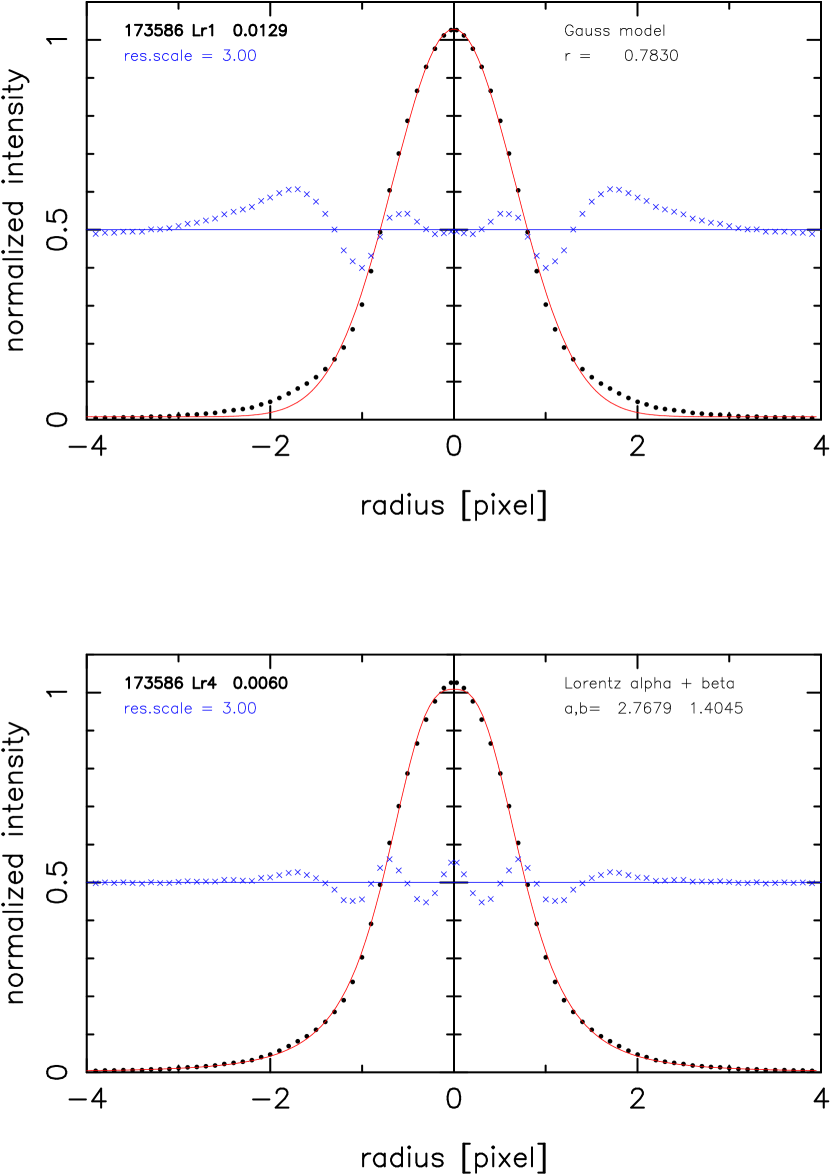
Figure 2: Radial profile plot of supersampled (see text) images on the left side of CCD frame 173586. The same data points are shown in both diagrams with a fit of a Gaussian (top) and Lorentz model function (bottom). Residuals are scaled with a factor of 3 and shown with an intensity offset of 0.5 for better readability.

Figure 2 shows the radial profile of a supersampled PSF (as explained above) obtained from stellar images on the left side (nearly no CTE effect) of CCD frame 173586 as an example. The same data points are shown in both plots. However, for the top plot the Gaussian (model 1) function was used to generate the fit line through the data points, while the bottom plot shows the result of model 4. A much better fit to the actual data is obtained with the latter model.

The small crosses running through the middle of each plot show the residuals (data $-$ fit model), scaled by a factor of 3 and offset by a constant along the intensity axis for better visualization. The Lorentz profile model gives significantly smaller residuals (about a factor of 2) than the Gaussian model; however, the Lorentz profile fit is not perfect either, and the spacial frequency of the residuals has increased, giving more peaks and valleys in the residual pattern, thus increasing its complexity.

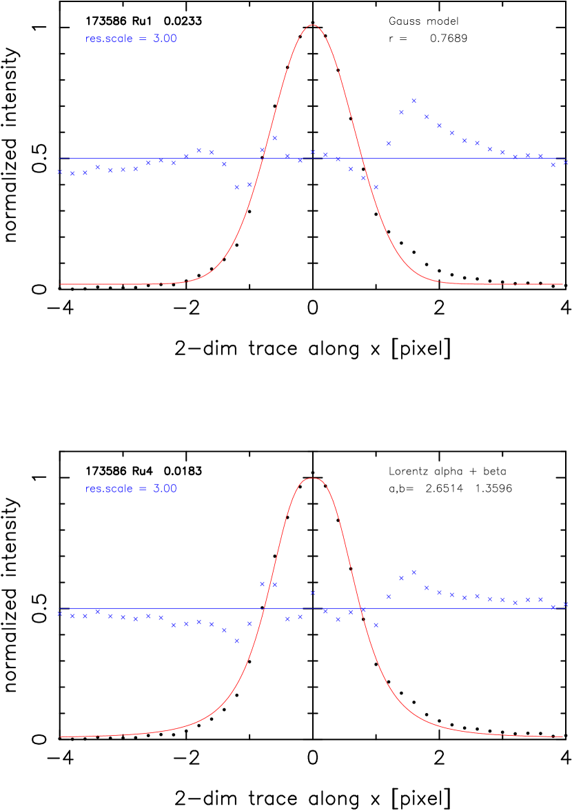
Figure 3: Profile plot along $x$-axis of supersampled images on the right side of CCD frame 173586. The same data points are shown in both diagrams with a fit of a Gaussian (top) and Lorentz model function (bottom). Residuals are scaled with a factor of 3 and shown with an intensity offset of 0.5 for better readability.

Figure 3 shows a similar set of plots obtained from the same CCD frame; however, using stellar images on the right side of the CCD (large CTE effect) and showing a marginal cut along $x$ instead of the radial coordinate used in Fig. 2. Clearly the asymmetry of the profile is seen, and both models perform about equally well, with a slightly better fit for the Lorentz model.

Figure 4 illustrates contour plots of residuals after fitting the supersampled PSF of the right side (large CTE effect) of frame 134473 (compare to Fig. 1). This asymmetric image could be fit reasonably well with model 9 using an elliptical, general, Lorentz profile function and asymmetry terms for $x$ (see Eq. 5), a total of 9 free parameters. The contour residuals using model 4 are shown for comparison. Residuals of a fit with model 1 look similar to the model 4 plot, although with larger amplitudes. In any case relatively large residuals with high spacial frequencies remain even when applying the asymmetric model.

4.4 Minimize number of free parameters

Fitting individual stellar images which extend only over a few pixels with models having 8 or even 10 free parameters, if numerically feasible at all, will lead to poor results in astrometry due to the small degree of overdetermination in the least-squares process. In order to benefit from the image profile models which better fit our data than the Gaussian some restrictions in parameter space were investigated.

A set of 282 high quality CCD frames was selected to sample the range in FWHM and span the entire observing epoch range. All these frames have a large number of stars, but are not crowded. For all frames the supersampling of the PSF was performed and various image profile fit models run on these, separately for each CCD frame. Results were summarized in a table and supplemented by observing log items.

Figure 5 shows the strongest correlation found for the various parameters investigated. The shape parameters ($\alpha,\beta$) of the symmetrical Lorentz profile model 4 can be predicted from the profile width of the Gaussian model 1 fit. The profile width here is the radius (about FWHM/2) with unit bin width (0.2 pixel) of the supersampled profile data. A linear term is sufficient to predict the $\beta$ parameter, while for the $\alpha$ parameter a second order polynomial was adopted. Scaling to the actual pixel size these results were hard-coded to preset both shape parameters in profile fit model 5, which is otherwise the same as model 4. This leaves only 5 free fit parameters, exactly the same as for the 2-dim Gaussian model function (see above and Table 1).

Tests were performed to determine any possible variations of the $\alpha$ and $\beta$ parameters. Supersampled PSFs were generated as a function of 2 magnitude bins, and in another test the data were split into 4 quadrants on the CCD frames. Consistent results for the $\alpha$ and $\beta$ parameters were found, confirming the relationship with the profile width as before with very small variation as a function of other selection criteria.

4.5 Other models

Tests were performed using elliptical profile models (6,7,8). No significant advantage was found over circular, symmetric models. The residuals similar to those shown in Fig. 4 did not generally decrease, unless the model was extended to include asymmetric terms in addition.

Asymmetric profiles were tested extensively on the supersampled PSF data of the selected frames used previously. In particular, model 12 was used to probe parameter space and look for dependencies. Smaller residuals than with any symmetric profile were found, however different parameter values are needed for stellar images in different locations on the detector as well as for different CCD frames.

Figures 6 and 7 show some examples obtained with test runs using models 9 and 11, respectively. The amplitude, $c_{x}$ (Eq. 6), of the asymmetric term along the $x$-coordinate (right ascension) is approximated by a function linear with air temperature and $x$ itself. Image profiles are symmetric at low $x$ and the largest asymmetry is seen at large $x$. Similarly the amplitude of the asymmetry along the $y$-coordinate was estimated as a linear function of temperature and $y$. Model 13 implements these preset values for $c_{x}$, and $c_{y}$, leaving only 6 free parameters, including the $a,b$ profile widths along $x$ and $y$, respectively (elliptical Lorentz base model).

4.6 Double star fits

Double star models solve simultaneously for at least 3 more parameters: the center coordinates, $x,y$ and amplitude, $A$ of the secondary component. Again, the goal is to minimize the number of free parameters as much as possible. Thus, for example, a single parameter for the background level is used. Some double star models also assume equal widths of the profiles of both components. Table 1 gives more details (models 20 to 23).

Critical for handling of blended images is the identification of such cases and the determination of sufficiently accurate starting parameters for the iterative, non-linear double star profile fit routine. This process can easily “go astray” due to the relatively large number of parameters and the small number of pixels available with the critically sampled UCAC data.

The adopted criterion for detecting an object on a dark and flat corrected CCD frame is to have at least 2 connected pixels above a specified S/N threshold level of $3\sigma$ above mean background. For each such detected object a centroid position (center-of-light, 1st moments) is calculated as well as the 2nd moments. The orientation of the major axis and image elongation, defined as the ratio of major to minor axis are derived from these moments. An elongation of 1.0 means a circular, symmetric image, otherwise the elongation is greater than 1. An image profile fit with model 1 (circular, symmetric Gaussian) is performed on all objects to identify “good” stars, and the mean image elongation of that CCD frame is calculated from the 2nd moment results of the “good” stars only. Images are typically slightly elongated due to guiding errors and the CTE effect.

The double star routines are triggered if an objects elongation exceeds an adopted threshold of 12% over the mean image elongation (for that CCD frame), and has a sufficient number of pixels ($\geq$10) above the detection threshold level. This elongation threshold was adopted as best compromise between excluding false positives of single stars due to statistics and including as many as possible real double stars. With some interpolation, pixel values are compared which lie on a line through the center of light along the major axis as determined earlier. A search is made for 2 peaks along this line and starting parameters (location and amplitudes) of the 2 components are derived. Starting parameters for the image profile width and background value are taken from the overall CCD frame mean values. If no 2 separate peaks can be detected, estimates for a possible nearby, blended, secondary component are made based on the image profile width and brightness of the object under investigation.

A least-squares fit is attempted with these starting parameters using model 23 (see Table 1), based on the Lorentz profile. The object is output as 2 components if reasonable starting parameters could be derived, even if the double star fit failed. A double star flag is assigned specifying the status of each successful detection and/or fit of 2 components.

A sample of newly detected UCAC3 doubles was observed with the 26-in speckle program Mason, Hartkopf & Wycoff (2008) and a paper addressing accuracy and reliability of UCAC3 double star data will be presented in a separate paper (Mason et al., 2010).

5 UCAC3 PIXEL REDUCTION RUN

5.1 Algorithm

The final reduction pipeline to process the UCAC3 pixel data handles a specified range of CCD frames with a single selected master flat and pairs of low/high ADU master dark frames for each standard exposure time (see above). The input list of frames is sorted by exposure time, and frames are then processed in that order, performing the following steps:

1. Read original, compressed pixel data file, determine mean left/right background counts and flag saturated pixels.

2. Interpolate dark frame, apply dark and flat corrections, output processed image (round to 2-byte integers).

3. Flag pixels from bad pixel maps, detect and flag possible streaks (from shutter failure and bleeding images).

4. Pass 1:

   1. Detect objects ($3\sigma$ above mean background for at least 2 connected pixels).

   2. Classify objects including 1st and 2nd moments, identify possible blended images (doubles).

   3. Perform image center fits on all objects with model 1 (Gaussian).

5. Intermission 1:

   1. Identify “good” stars over entire CCD frame, based on model 1 fit results.

   2. Derive mean image profile width, mean image elongation, $\alpha,\beta$ profile shape parameters, and radii for aperture photometry.

6. Pass 2:

   1. Perform circular, symmetric Lorentz profile fit (model 5).

   2. Calculate double star starting parameters and perform fit (model 23).

   3. Perform asymmetric profile fit (model 13).

7. Intermission 2:

   1. Select “good” stars from model 13 fit results.

   2. Derive mean width of profiles ($a,b$) of elliptical part of model 13 and fixed parameters for model 14.

8. Pass 3: Perform model 14 fit with further parameter restrictions.

9. Perform aperture photometry.

10. Derive model magnitudes from each successful model fit.

11. Output all fit results for each frame to a separate file.

The profile fits are performed with pixels inside a circular aperture centered on the best known position at the time. The radius of this aperture was adopted to be twice as large as the radius of the area of pixels above the threshold from the image detection step. For all astrometric image profile fits the local background parameter is a free fit parameter for each single star or binary pair.

Note, the astrometric fit based on the Lorentz profile is performed with 5 free parameters, the same number of parameters as used for a Gaussian profile model. The major difference is that here a model profile is selected that does better match the data with the profile shape being slightly different for CCD frames taken under different seeing conditions (average image width). The first step in this reduction process (finding $\alpha,\beta$) merely is a quantitative way to make a “good guess” about which model profile to use.

For the aperture photometry all pixels within 4 times the mean radius of the image profiles (Gaussian fit of “good” stars) of that CCD frame were used to determine the flux of a target. An annulus with 12 and 16 times this mean profile radius served for the background determination. The background value is determined from the peak of the histogram of background pixels (weighted mean of bins which exceed 50% of the smoothed histogram peak value).

5.2 Processing and Results

The re-processing of the pixel data involved 5 different Linux workstations (mostly single processor at about 2 GHz), which most of the time ran in parallel for about a month working on a section of the UCAC frames each. Individual binary files contain the output data for each CCD frame. The number of objects per frame ranged from 37 to 75,549 with a median of 1397. A data record of 136 bytes contains the results for each detected object, including selected items from the moment analysis, the parameters of the 4 model fits, their errors, and flags. Data items were converted to integers of 1, 2, or 4 byte lengths with appropriate scaling. A total of over 4 TB of compressed pixel data went into this process, producing a total of 80 GB of binary $x,y$ data, the results of 271,428 CCD exposures. These files were later extended by 8 bytes per record to arrive at the final $x,y$-data output files. The additional data contain information about nearest neighbors, and identification of possible doubles that are not blended.

5.3 Analysis of the Results

How good are the resulting $x,y$ data? An example of the internal fit precision is presented in Figure 8. The formal standard error of the $x$-center coordinate is shown as a function of instrumental magnitude. Data for the same CCD frame are shown for 3 different image profile fit models (1, 5, and 14). The results for model 13 look very similar to those of model 14. The results for the $y$ coordinate are similar to those of the $x$-coordinate. Saturation occurs at about magnitude 8. The unit is milli pixel (mpx), with 1 mpx = 0.9 mas. For the unsaturated, high S/N stars (8 to 10 mag) per coordinate precisions of about 6 mpx, 4 mpx, and 3 mpx are reached for fit models 1, 5, and 14, respectively, from a single CCD frame observation of good quality.

The repeatability of observations was tested frequently with the same field in the sky observed twice within minutes and the telescope being on the same side of the pier. A weighted, linear transformation between the sets of $x,y$ data of such a pair of 100 s exposures was performed and the scatter in the $x$ coordinate of stars plotted as a function of instrumental magnitude in Figure 9. Again, results from different profile fit models (pfm) are shown as indicated. This scatter includes the errors from both CCD frames. Assuming equal error contribution, the repeatability error of these observations is thus about 15 mpx / $\sqrt{2}$ $\approx$ 11 mpx $\approx$ 10 mas per coordinate and single observation for well exposed stars, almost independent of the profile fit model. These results are consistent with the first observations at this telescope using a CCD camera (Zacharias, 1997). The observed error is significantly larger than the internal fit precision (of bright stars) due to atmospheric turbulence. A scatter that is about a factor of 2 larger is observed in similar CCD frame pairs of 25 s exposure time as compared to the 100 s frames.

The flip observations, with the telescope on one side of the pier then on the other, provide pairs of frames that are rotated by $180^{\circ}$ with respect to each other. A linear transformation between the 2 sets of $x,y$ data of each frame pair taken on the same field in the sky gives residuals revealing systematic errors as a function of magnitude or coma-like terms (product of magnitude and positional coordinates). An example is shown in Figure 10 for such a pair of frames with 100 s exposure, before applying corrections. Results are derived from the same pixel data but using all 4 different profile fit models as indicated. Each data point is the mean for 16 stars. The model 5 and 13 results show a somewhat tighter distribution than those of models 1 and 14. Unfortunately a similar amplitude of the systematic errors is present in the data from all 4 models, while the hope has been that the asymmetric profile fits would have mitigated this problem. Even larger systematic errors (about 200 mas) are seen in short exposure frames. These and other systematic errors will be investigated in great detail with the help of reference stars, as described in another paper of this series (Finch, Zacharias & Wycoff, 2010). Empirical corrections will be derived for these and other systematic errors in the UCAC data at that time. These corrections effectively reduce these types of systematic errors by about a factor of 10 (as compared to what is seen in Fig. 10) for the published catalog star positions.

6 DISCUSSION AND CONCLUSIONS

The detection threshold for blended, double star images is affected by the gradient of inherent image elongation along the $x$ axis due to the poor CTE. Similarly fit results of double stars will have a slight bias depending on the $x$ pixel coordinate. Almost symmetric images are seen on the left side of a CCD frame, while CTE elongated, asymmetric images are seen on the right side. In all cases the same, symmetric double star profile is used for a fit. In addition, a slight image elongation is typically added from guiding effects. Nevertheless, an important first step for detecting double stars and deriving useful parameters has been accomplished for UCAC3. Results from external comparisons will be presented in (u3d).

The additional first order parameters to describe image asymmetry (relative amplitude of a term linear with pixel coordinate) could not be correlated well to any other parameters, contrary to the $\alpha$ and $\beta$ shape parameters used in the Lorentz profile model. Even such a complex model applied without approximations of the asymmetric parameters (i.e. use of many free fit parameters) leaves significantly large residuals (see Fig. 4 bottom) in the supersampled, stacked PSFs. Applying a model with 7 or more parameters to the (not supersampled) original pixel data for each star is not an option with the critical sampling of the UCAC data (too few pixels per image).

This situation calls for a purely empirical PSF model by using the supersampled, stacked, observed profiles to generate a template. Using purely empirical PSFs as templates to fit observed stellar images in UCAC data, however, was not considered a viable option. Many UCAC frames have a low number of stars, in particular the number of stars with high S/N ratio needed for this approach is very small (a few) in many areas of the sky. Furthermore, the PSF changes significantly over the area of the detector (mainly along the $x$ coordinate) due to the poor CTE and, is a function of the profile width (FWHM), the guiding of each exposure, the CCD temperature and probably other factors. Splitting up the data into so many categories was not an option. In general a purely empirical PSF will be asymmetric to some degree, also caused by imperfect guiding. Such an approach would mean a different definition of an image center for different CCD frames with additional variations over the field of view, not desirable for astrometry. Thus the use of models 13 and 14 is a compromise driven by the need for a more complex model without having a large enough sampling to support it.

The very high precision of the well exposed stellar images seen in the internal fit errors per coordinate unfortunately does not translate into similarly small external errors. Internal errors of under 5 mas per coordinate and exposure are seen, however the repeatability of such observations is already degraded to about 10 mas and more due to the atmosphere for our long exposures of 100 to 150 s. For the short exposures the positional errors are further increased by about a factor of 2. However, the UCAC data are still limited by remaining systematic errors, resulting in an error floor of just under 20 mas per coordinate for the mean CCD observations (4 images) for stars in the R = 10 to 14 mag range, as will be shown in the astrometric reduction paper (Finch, Zacharias & Wycoff, 2010).

The symmetric profile model 5 $x,y$ center coordinates have been adopted as the baseline for these astrometric reductions. It could be argued that the derived $\alpha$ and $\beta$ shape parameters used in model 5 are not accurately enough known, based on the approximation as described above. However, very good astrometric results have already been obtained with the Gaussian model (UCAC2, and many other traditional, astrometric catalog projects). The Lorentz profile adopted here, with a somewhat imperfect representation of shape parameters, is a far better representation of the observed image profile than is the Gaussian model. Both are symmetric profile functions with the same number of free parameters, so no detrimental effect is expected when choosing model 5 (Lorentz profile) over model 1 (Gauss profile).

Effects from image asymmetry will be investigated and corrected by analyzing the residuals with respect to reference stars. No significant benefit for the overall astrometric accuracy has been found so far by using the asymmetric profile models investigated here, particularly with respect to solving magnitude and coma-like terms. For the baseline UCAC reductions a symmetric PSF model is applied to asymmetric image profiles with subsequent systematic error corrections of the celestial coordinates using reference stars.

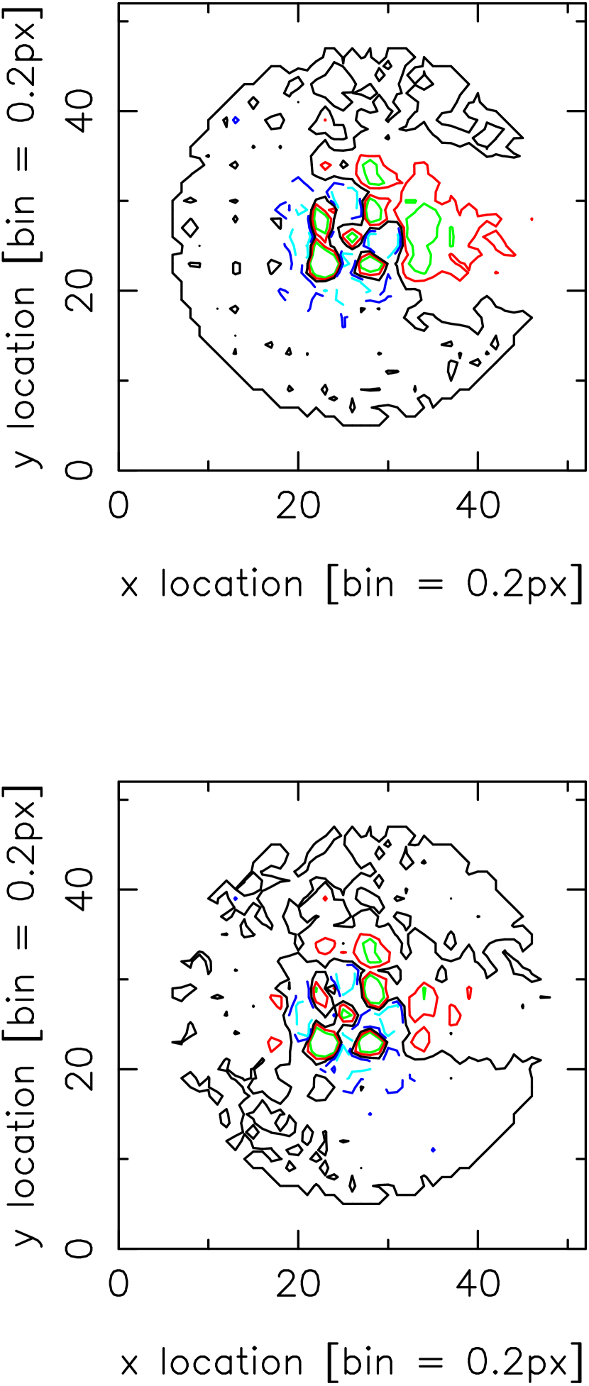
Figure 4: Residual contour plot of a supersampled PSF from stellar images on the right side of CCD frame 134473. The same data are used for both plots; model 4 (symmetric Lorentz profile) fit (top), and model 9 (elliptic Lorentz profile plus asymmetry terms along $x$) (bottom) fits were applied, respectively. Contour levels are light blue $-3$%, dark blue $-1.5$%, black 0, red $+1.5$%, and green $+3$%.

Figure 5: Alpha (top) and beta (bottom) image profile shape parameters of the Lorentz model 4 as a function of the image width (radius) as determined by model 1 (Gauss) for the supersampled data (1 bin = 0.2 pixel). The alpha parameter is fit by a 2nd order polynomial, while the beta parameter is well represented by a linear dependency.

Figure 6: Examples of the asymmetry along $x$ parameter dependencies from supersampled data. The amplitude of the asymmetry along $x$ (RA) as a function of the air temperature (bottom) and as a function of the image profile radius (top) are among the strongest correlations found.

Figure 7: Similarly to the previous figure, the dependency of the amplitude of image asymmetry along $y$ (Dec) is shown here.

Figure 8: Internal fit precision (milli pixel = 0.9 mas) along the $x$ coordinate as a function of aperture magnitude of a long exposure sample frame 53554 with over 4000 stars. The plots zoom in on the high precision, high S/N area (bright stars). Results for different fit models are shown: model 1 (Gaussian) on top, model 5 (Lorentz) in the middle, and model 14 (asymmetric profile) on the bottom.

Figure 9: Standard error (sigma) of the $x$ coordinate as a function of instrumental model magnitude from the comparison of 2 100-second exposures taken of the same field in the sky within minutes. Results are shown from the same CCD frame pair but for different image profile fit models (pfm) as indicated. The error shown is the combined error of both exposures, dominated by atmospheric effects. Each dot represents the RMS average of 16 stars. Unit is milli pixel (1 mpx = 0.9 mas).

Figure 10: Systematic differences between the $x$ coordinates of a pair of 100-second exposures taken from opposite sides of the telescope pier (rotated by $180^{\circ}$ with respect to each other) as a function of instrumental model magnitude, after a linear transformation of the $x,y$ data but without any other corrections applied. Results are shown from the same CCD frame pair but for different image profile fit models (pfm) as indicated. Each dot represents the mean over 16 stars. Unit is milli pixel (1 mpx = 0.9 mas).

Table 1: Description of image profile models used in UCAC3 reductions and tests.

profile fit model number

1

2

3

4

5

6

7

8

9

10

11

12

13

14

20

21

22

23

base model

G

D

L

L

L

G

G

L

L

L

L

L

L

L

Gd

Gd

Ld

Ld

symmetry

c

c

c

c

c

e

e

e

e,a

e,a

e,a

e,a

e,a

e,a

c

c

c

c

total number of parameters

5

6

7

7

7

6

7

8

9

9

9

10

10

10

8

9

11

11

numb.of free fit parameters

5

6

6

7

5

6

7

8

9

7

9

8

6

4

8

9

9

8

$x,y$ center, ampl., backgr.

f

f

f

f

f

f

f

f

f

f

f

f

f

f

f

f

f

f

profile width

f

f

f

f

f

f

f

f

f

f

f

f

f

p

f

f

f

f

elliptical axis orientation

f

1st shape parameter

f

f

f

p

f

f

p

f

p

p

p

p

p

2st shape parameter

p

f

p

f

f

p

f

p

p

p

p

p

asymmetry $x$ amplitude

f

f

f

p

p

asymmetry $y$ amplitude

f

f

p

p

$x,y$, amplitude secondary

f

f

f

f

profile width secondary

f

f

References

- Anderson & King (2000) Anderson, J. & King, I. R. 2000, PASP, 112, 1360
- Finch, Zacharias & Wycoff (2010) Finch, C., Zacharias, N., & Wycoff, G. L. 2010, in press, AJ
- Mason, Hartkopf & Wycoff (2008) Mason, B. D., Hartkopf, W. I., & Wycoff, G. L. 2008, AJ, 136, 2223
- Mason et al. (2010) Mason, B. D. et al., observations of UCAC3 double stars, in prep.
- Moffat (1969) Moffat, A. F. J. 1969, A&A, 3, 455
- Stetson (1987) Stetson, P. B. 1987, PASP, 99, 101
- Schramm (1998) Schramm, J. 1998, Ph.D. thesis, Hamburg Observatory
- Winter (1999) Winter, L. 1999, Ph.D. thesis, Hamburg Observatory
- Zacharias (1997) Zacharias, N., 1997, AJ, 113, 1925
- Zacharias et al. (2000) Zacharias, N., Zacharias, M. I., & Rafferty, T. J. 2000, AJ, 118, 2503
- Zacharias et al. (2004) Zacharias, N., Urban, S. E., Zacharias, M. I., Wycoff, G. L., Hall, D. M., Monet, D. G., & Rafferty, T. J. 2004, AJ, 127, 3043
- Zacharias et al. (2010) Zacharias, N. et al. 2010, submitted to AJ