Combined Constraints on Holographic Bosonic Technicolor

Abstract

We consider a model of strong electroweak symmetry breaking in which the expectation value of an additional, possibly composite, scalar field is responsible for the generation of fermion masses. The dynamics of the strongly coupled sector is defined and studied via its holographic dual, and does not correspond to a simple, scaled-up version of QCD. We consider the bounds from perturbative unitarity, the $S$ parameter, and the mass of the Higgs-like scalar. We show that the combination of these constraints leaves a relatively limited region of parameter space viable, and suggests the qualitative features of the model that might be probed at the LHC.

I Introduction

The physics of electroweak symmetry breaking (EWSB) will soon be probed directly at the Large Hadron Collider (LHC). One logical possibility is that the sector responsible for electroweak symmetry breaking will involve new, nonperturbative dynamics. Historically, technicolor models have represented an attempt at constructing viable theories of this type technicolor .

Conventional technicolor models, however, suffer from a number of well-known problems. As originally proposed, the technicolor sector was assumed to be a scaled-up version of QCD, leading to estimates for the $S$ parameter that are unacceptably large PT . In addition, an extended technicolor (ETC) sector must be added to generate the operators needed to account for Standard Model fermion masses etc . In many ETC models, it is impossible to account for a heavy top quark (which requires the ETC scale to be low) and suppress other ETC operators that contribute to flavor-changing-neutral-current (FCNC) processes (which requires the ETC scale to be high). Viable and elegant ETC models have been few and far between.

Developments over the last decade in the physics of higher-dimensional and conformal field theories, however, have led to new possibilities in technicolor model building hong ; sanz ; cet1 ; acgr ; cesh ; hirayama ; haba ; piai ; dandk ; mint ; kit ; round ; belitsky ; supertc ; luty ; also . For example, the magnitude of the $S$ parameter in QCD-like technicolor theories suggests one should not exclusively study theories that are exactly like QCD (as, for example, in Refs. sanz or cet1 ). A decade or so ago, this would have been a fruitless effort. Now, the AdS/CFT correspondence adscft provides a means of constructing a perturbative, five-dimensional (5D) theory that is dual to a strongly coupled technicolor theory localized on a four-dimensional (4D) boundary hong ; sanz ; cet1 ; acgr ; cesh ; hirayama ; haba ; piai ; dandk ; mint ; kit ; round ; belitsky . For some values of the parameters that define the 5D theory, the dual theory can model a scaled-up version of QCD. However, for other parameter choices it does not. In either case, observables can be computed reliably in the 5D theory, which we can think of as defining its strongly coupled dual. The freedom to deviate from the QCD-like limit only presumes the validity of a gauge/gravity correspondence. The evidence for this is not insignificant, and includes holographic models of QCD phenomenology that agree remarkably well with the low-energy data adsqcd ; eandw .

The problem with fermion mass generation in the conventional ETC framework, on the other hand, may suggest something about the form of the relevant low-energy effective theory. It was observed long ago that a techniquark bound state with the same quantum numbers as a Standard Model Higgs doublet can form in ETC models in which the ETC gauge coupling becomes strong setc ; this bound state has Yukawa couplings to the Standard Model fermions and may develop a vacuum expectation value, producing fermion masses. The low-energy effective theory, taken by itself, has no problems with FCNC effects, since these originate from scalar-exchange diagrams that are no larger than in conventional two-Higgs doublet models. A significant number of phenomenological studies on such “bosonic technicolor” scenarios were motivated by the simplicity of this low-energy effective theory bt1 ; bt2 ; bt3 ; bt4 ; bt5 ; bt6 ; bt7 ; bt8 ; bt9 . While bosonic technicolor can arise from a (fine-tuned) strongly coupled ETC model, the low-energy effective theory is by no means linked uniquely to that ultraviolet completion. For example, the same effective theory can arise in a warped, 5D theory with a Higgs field localized near the Planck brane and symmetry-breaking boundary conditions on the bulk gauge fields acgr . In this setting, the presence of a scalar in the spectrum of the theory seems far from scandalous. The value of working with the low-effective effective description is that one can extract robust, low-energy predictions of the theory without being hindered unnecessarily by one’s ignorance of the physics that has decoupled in the ultraviolet.

It is such robust predictions of the low-energy effective theory that are of interest to us in this paper. Using the holographic approach to define our strongly coupled sector, and the associated freedom to deviate from the limit in which this sector is like QCD, we show that the parameter space of the theory is nonetheless significantly constrained. Combining the bounds on the $S$ parameter (evaluated holographically), partial-wave unitarity in longitudinal $W$ boson scattering (with the technirho couplings evaluated holographically) and the bound on the mass of the light Higgs-like scalar (with a relevant chiral Lagrangian parameter evaluated holographically), we find that there is a relatively narrow region of parameter space in which the model is currently viable. In deforming the theory away from its QCD-like limit, we focus primarily on varying the ratio of the chiral symmetry breaking to the confinement scale, as well as the amount of explicit chiral symmetry breaking originating from the current techniquark masses. In addition, bosonic technicolor models allow one to vary the symmetry breaking scale associated with the strongly interacting sector, while holding the electroweak scale fixed. Within the allowed parameter region, the ranges of observable quantities are substantially restricted, suggesting the qualitative features of the model that may be relevant at the LHC. The new results presented here suggest that the simplest version of holographic bosonic technicolor may be sufficiently constrained that upcoming collider data could soon render debates on the possible origins of the effective theory largely irrelevant.

Our paper is organized as follows. In the next section, we review the relevant low-energy effective theory. In Sections III and IV, we discuss the holographic calculations of the observable quantities that we use to constrain the parameter space of the theory. In Section V, we present our numerical results and in Section VI we summarize our conclusions.

II The Model

The gauge group of the model is $G_{\rm TC}\times\textrm{SU}(3)_{C}\times\textrm{SU}(2)_{W}\times\textrm{U}(1)_{Y}$, where $G_{\rm TC}$ represents the technicolor group. We will assume that $G_{TC}$ is asymptotically free and confining. We assume two flavors of technifermions, $p$ and $m$, that transform in the $N$-dimensional representation of $G_{\rm TC}$. In addition, these fields form a left-handed $\textrm{SU}(2)_{W}$ doublet and two right-handed singlets,

$$\Upsilon_{L}\equiv\left(\begin{array}[]{c}p\\ m\end{array}\right)_{L},\,\,\,\,\,p_{R},\,\,\,\,\,m_{R},$$ (1)

with hypercharges $Y(\Upsilon_{L})=0$, $Y(p_{R})=1/2$, and $Y(m_{R})=-1/2$. With these assignments, the technicolor sector is free of gauge anomalies. With $N$ even, the SU(2) Witten anomaly is also absent.

The technicolor sector has a global $\textrm{SU}(2)_{L}\times\textrm{SU}(2)_{R}$ symmetry that is spontaneously broken when the technifermions form a condensate

$$\left<\bar{p}p+\bar{m}m\right>=\sigma_{0}\,\,\,.$$ (2)

The electroweak gauge group of the Standard Model is a subgroup of the chiral symmetry; $\textrm{SU}(2)_{W}$ is isomorphic to $\textrm{SU}(2)_{L}$, while $\textrm{U}(1)_{Y}$ is identified with the third generator of $\textrm{SU}(2)_{R}$. The condensate breaks $\textrm{SU}(2)_{W}\times\textrm{U}(1)_{Y}$ to $\textrm{U}(1)_{\rm EM}$ and generates $W$ and $Z$ masses. However, additional physics is required to communicate this symmetry breaking to the Standard Model fermions. Bosonic technicolor models utilize the simplest possibility, a scalar field $\phi$, that transforms as an $\textrm{SU}(2)_{W}$ doublet with hypercharge $Y(\phi)=1/2$. The scalar has Yukawa couplings to both the technifermions,

$$\mathcal{L}_{\phi T}=-\bar{\Upsilon}_{L}\tilde{\phi}\,h_{+}p_{R}-\bar{\Upsilon}_{L}\phi\,h_{-}m_{R}+{\rm h.c.},$$ (3)

and to the ordinary fermions,

$$\mathcal{L}_{\phi f}=-\bar{L}_{L}\phi h_{l}E_{R}-\bar{Q}_{L}\tilde{\phi}h_{U}U_{R}-\bar{Q}_{L}\phi h_{D}D_{R}+{\rm h.c.},$$ (4)

where $\tilde{\phi}=i\sigma^{2}\phi^{*}$. Unlike the Standard Model Higgs doublet, the $\phi$ field is assumed to have a positive squared mass. When the technifermions condense, Eq. (3) produces a $\phi$ tadpole term in the scalar potential, and $\phi$ develops a vacuum expectation value, as we will see in a more conventient parameterization below. Standard Model fermion masses then follow from the Yukawa couplings in Eq. (4).

To be more explicit, we use the conventional nonlinear representation of the Goldstone bosons to construct the electroweak chiral Lagrangian. We define

$$\Sigma=\exp(2i\Pi/f),\,\,\,\,\,\Pi=\left(\begin{array}[]{cc}\pi^{0}/2&\pi^{+}/\sqrt{2}\\ \pi^{-}/\sqrt{2}&-\pi^{0}/2\end{array}\right)\,,$$ (5)

where $\Pi$ represents an isotriplet of technipions, and $f$ is their decay constant. The $\Sigma$ field transforms under $\textrm{SU}(2)_{L}\times\textrm{SU}(2)_{R}$ as

$$\Sigma\rightarrow L\,\Sigma\,R^{\dagger}\,,$$ (6)

which dictates the form of the pion interactions. To include the scalar doublet consistently in the effective theory, it is convenient to use the matrix form

$$\Phi=\left(\begin{array}[]{cc}\overline{\phi^{0}}&\phi^{+}\\ -\phi^{-}&\phi^{0}\end{array}\right).$$ (7)

The technifermion Yukawa couplings can be re-expressed as

$$\overline{\Upsilon}_{L}\left(\begin{array}[]{cc}\overline{\phi^{0}}&\phi^{+}\\ -\phi^{-}&\phi^{0}\end{array}\right)\left(\begin{array}[]{cc}h_{+}&0\\ 0&h_{-}\end{array}\right)\Upsilon_{R}\equiv\overline{\Upsilon}_{L}\Phi H\Upsilon_{R}.$$ (8)

Since the underlying theory would be invariant if the combination $\Phi H$ transformed as

$$(\Phi H)\rightarrow L\,(\Phi H)\,R^{\dagger},$$ (9)

one may correctly include this combination in the effective theory by assuming it transforms in this way. The lowest-order term in the electroweak chiral Lagrangian that involves $\Phi H$ is

$$\mathcal{L}_{H}=c_{1}4\pi f^{3}\textrm{Tr}(\Phi H\Sigma^{\dagger})+h.c.\;,$$ (10)

where $c_{1}$ is an unknown, dimensionless coefficient; one expects $c_{1}$ to be of order one by naive dimensional analysis Manohar:1983md in a QCD-like theory. Henceforth, we assume that $h_{+}=h_{-}\equiv h$, to simplify the parameter space of the model.

It is convenient to re-express the $\Phi$ field using a nonlinear field redefinition, similar to Eq. (5). Expanding about the true vacuum,

$$\Phi=\frac{\sigma+f^{\prime}}{\sqrt{2}}\Sigma^{\prime},\,\,\,\,\,\Sigma^{\prime}=\exp(2i\Pi^{\prime}/f^{\prime})\,,$$ (11)

where $f^{\prime}$ is the vev of $\phi$ and $\Pi^{\prime}$ represents its isotriplet components. The kinetic terms for the $\Phi$ and $\Sigma$ fields can be written

$$\mathcal{L}_{KE}=\frac{1}{2}\partial_{\mu}\sigma\partial^{\mu}\sigma+\frac{f^{2}}{4}\textrm{Tr}(D_{\mu}\Sigma^{\dagger}D^{\mu}\Sigma)+\frac{(\sigma+f^{\prime})^{2}}{4}\textrm{Tr}(D_{\mu}\Sigma^{\prime\dagger}D^{\mu}\Sigma^{\prime}),$$ (12)

where the covariant derivative is given by

$$D^{\mu}\Sigma=\partial^{\mu}\Sigma-igW_{a}^{\mu}\frac{\tau^{a}}{2}\Sigma+ig^{\prime}B^{\mu}\Sigma\frac{\tau^{3}}{2}.$$ (13)

In the expansion of Eq. (12), there are quadratic terms that mix the gauge fields with derivatives of a specific linear combination of the pion fields:

$$\pi_{a}=\frac{f\,\Pi+f^{\prime}\,\Pi^{\prime}}{\sqrt{f^{2}+f^{\prime 2}}}.$$ (14)

The mixing indicates that the components of $\pi_{a}$ are unphysical and can be gauged away. On the other hand, the orthogonal linear combination,

$$\pi_{p}=\frac{-f^{\prime}\,\Pi+f\,\Pi^{\prime}}{\sqrt{f^{2}+f^{\prime 2}}}\,,$$ (15)

represents physical states in the low-energy theory. The physical pion mass is determined from Eq. (10):

$$m_{\pi}^{2}=8\sqrt{2}\pi c_{1}h\frac{f}{f^{\prime}}v^{2}\,.$$ (16)

In unitary gauge, the remaining quadratic terms give the masses of $W$ and $Z$ bosons,

$$m_{W}^{2}=\frac{1}{4}g^{2}v^{2},\,\,\,\,\,\,\,\,\,\,m_{Z}^{2}=\frac{1}{4}(g^{2}+g^{\prime 2})v^{2},$$ (17)

where $v$ represents the electroweak scale

$$v\equiv\sqrt{f^{2}+f^{\prime 2}}=246\textrm{ GeV}.$$ (18)

In the absence of a technicolor sector, with $f^{\prime}=v$, the $\sigma$ field corresponds to the Higgs boson of the Standard Model. Away from this limit, the $\sigma$ field is similar to a Standard Model Higgs boson, but with different couplings. Expanding the third term of Eq. (12), we find that the coupling between $\sigma$ and the gauge bosons is given by

$$\mathcal{L}_{\sigma WZ}=2\frac{f^{\prime}}{v}\frac{m_{W}^{2}}{v}\sigma W^{+\mu}W_{\mu}^{-}+\frac{f^{\prime}}{v}\frac{m_{Z}^{2}}{v}\sigma Z^{\mu}Z_{\mu}\,,$$ (19)

which is reduced by a factor of $f^{\prime}/v$ compared to the result in the Standard Model. The couplings of the $\Phi$ field to the quarks is given by

$$\mathcal{L}_{\Phi\bar{q}q}=-\bar{\psi}_{L}\Phi\left(\begin{array}[]{cc}h_{U}&0\\ 0&V_{CKM}h_{D}\end{array}\right)\psi_{R}+\textrm{h.c.}\ ,$$ (20)

where $\psi_{L}=(U_{L},V_{CKM}D_{L})$, $\psi_{R}=(U_{R},D_{R})$, $h_{U}=\textrm{diag}(h_{u},h_{c},h_{t})$, and $h_{D}=\textrm{diag}(h_{d},h_{s},h_{b})$. Using Eq. (11), this may be written

$$\mathcal{L}_{\Phi\bar{q}q}=-\frac{\sigma+f^{\prime}}{\sqrt{2}}\bar{\psi}_{L}\Sigma^{\prime}\left(\begin{array}[]{cc}h_{U}&0\\ 0&V_{CKM}h_{D}\end{array}\right)\psi_{R}+\textrm{h.c.}$$ (21)

Taking into account the leptons, the coupling of the $\sigma$ field to fermions is given by

$$\mathcal{L}_{\sigma\bar{f}f}=-\sum_{\textrm{fermions}}\frac{v}{f^{\prime}}\frac{m_{f}}{v}\sigma\bar{f}f\,.$$ (22)

Eq. (22) is larger than the corresponding result in the Standard Model by a factor of $v/f^{\prime}$; this enhancement corresponds to the larger Yukawa couplings that are required when electroweak symmetry breaking comes mostly from the strongly coupled sector.

III Holographic Calculations

We model the technicolor sector using the AdS/CFT correspondence adscft , which allows us to numerically evaluate the otherwise undetermined coefficients of the electroweak chiral Lagrangian, such as the parameter $c_{1}$ of Eq. (10). The AdS/CFT correspondence conjectures a duality between a 5D theory in anti-de Sitter (AdS) space and 4D conformal field theory (CFT) located on a boundary. For theories like QCD that are confining, the metric is a slice of AdS space:

$$ds^{2}=\frac{1}{z^{2}}\left(-dz^{2}+dx^{\mu}dx_{\mu}\right),\ \epsilon\leq z\leq z_{m}.$$ (23)

The position in the fifth dimension $z$ corresponds to the energy scale in the 4D theory; branes at $z=\epsilon$ and $z_{m}$ correspond to the ultraviolet (UV) and infrared (IR) cutoffs of the dual theory. The AdS/CFT correspondence dictates that operators in the boundary theory correspond to bulk fields in the 5D theory. To be more precise, given an operator $\mathcal{O}$ with the source $\phi_{0}(x)$, the generating functional in the 4D quantum field theory, $W_{4D}$, is given by the classical action of the 5D theory written in terms of the boundary value of the corresponding bulk field, $\phi(x,z)$:

$$W_{4D}[\phi_{0}(x)]=S_{5D}^{\rm class}|_{\phi(x,\epsilon)=\phi_{0}(x)}.$$ (24)

In addition, the AdS/CFT correspondence identifies each global symmetry in the boundary theory with a gauge symmetry in the 5D theory. The 5D action that describes the technicolor sector of our model is

$$S_{5D}=\int d^{5}x\sqrt{g}\;\textrm{Tr}\left\{-\frac{1}{2g_{5}^{2}}(F_{R}^{2}+F_{L}^{2})+|DX|^{2}+3|X|^{2}\right\}\,.$$ (25)

The chiral symmetry of the technicolor sector corresponds to the SU(2)${}_{L}\times$SU(2)_R gauge symmetry of the 5D theory, with gauge fields $A_{L,R}=A^{a}_{L,R}t^{a}$, where the $t^{a}$ are generators of SU(2) with ${\rm Tr}\,t^{a}t^{b}=\delta^{ab}/2$. The covariant derivative and field strength tensors are defined by $D_{\mu}X=\partial_{\mu}X-iA_{L\mu}X+iXA_{R\mu}$ and $F_{L,R\;\mu\nu}=\partial_{\mu}A_{L,R\;\nu}-\partial_{\nu}A_{L,R\;\mu}-i\left[A_{L,R\;\mu},A_{L,R\;\nu}\right]$. The scalar field $(2/z)X$ corresponds to the operator $\bar{q}_{R}q_{L}$, while the gauge fields $A_{L,R\;\mu}^{a}$ correspond to the chiral currents $\bar{q}_{L,R}\gamma^{\mu}t^{a}q_{L,R}$.

The equations of motion for the $X$ field may be solved, subject to the UV boundary condition $2/\epsilon\,X(\epsilon)=m_{q}$:

$$X(z)=\frac{1}{2}(m_{q}z+\sigma_{c}z^{3})\equiv\frac{1}{2}X_{0}(z).$$ (26)

The techniquark mass $m_{q}$ is related to the parameter $h$ by $m_{q}=h\,f^{\prime}/\sqrt{2}$. The coefficient $\sigma_{c}$ is equal to the condensate $\sigma_{0}$ (defined in Eq. (2)) when $m_{q}=0$, as can be shown by varying the action with respect to $m_{q}$ and then taking the chiral limit. More generally, $\sigma_{c}$ is a parameter that defines the holographic theory that we will eliminate in terms of the technipion decay constant $f$, as we discuss below.

We work with the vector and axial vector fields $V=(A_{L}+A_{R})/\sqrt{2}$ and $A=(A_{L}-A_{R})/\sqrt{2}$, respectively. The bulk-to-boundary propagator $V(q,z)$ is defined as the solution to the transverse equations of motion with $V_{\mu}(q,z)_{\perp}\equiv V(q,z)V_{\mu}(q)_{\perp}$ and $V(q,\epsilon)=1$, where $\epsilon$ is the UV boundary. From Eq. (25), it follows that the bulk-to-boundary propagators satisfy

$$\partial_{z}\left(\frac{1}{z}\partial_{z}V(q,z)\right)+\frac{q^{2}}{z}V(q,z) = 0\,,$$ (27)

$$\partial_{z}\left(\frac{1}{z}\partial_{z}A(q,z)\right)+\frac{q^{2}}{z}A(q,z)-\frac{g_{5}^{2}X_{0}(z)^{2}}{2z^{3}}A(q,z) = 0.$$ (28)

In accordance with Eq. (24), the vector and axial vector two-point functions are given holographically by adsqcd

$$\Pi_{V}(-q^{2})=\left.\frac{2}{g_{5}^{2}}\frac{1}{z}\frac{\partial V(q,z)}{\partial z}\right|_{z=\epsilon},\ \ \ \Pi_{A}(-q^{2})=\left.\frac{2}{g_{5}^{2}}\frac{1}{z}\frac{\partial A(q,z)}{\partial z}\right|_{z=\epsilon}.$$ (29)

where

$$\int d^{4}x\,e^{iq\cdot x}\left<J_{V}^{a\,\mu}(x)J_{V}^{b\,\nu}(0)\right> \equiv \delta^{ab}\left(\frac{q^{\mu}q^{\nu}}{q^{2}}-g^{\mu\nu}\right)\Pi_{V}(-q^{2})\,,$$

$$\int d^{4}x\,e^{iq\cdot x}\left<J_{A}^{a\,\mu}(x)J_{A}^{b\,\nu}(0)\right> \equiv \delta^{ab}\left(\frac{q^{\mu}q^{\nu}}{q^{2}}-g^{\mu\nu}\right)\Pi_{A}(-q^{2}).$$ (30)

Comparing $\Pi_{V}$ with the known perturbative result for an SU($N$) gauge theory, valid at high $q^{2}$, one finds adsqcd

$$g_{5}^{2}=\frac{24\pi^{2}}{N}\,.$$ (31)

We discuss this assumption further in the section on our numerical results. With the holographic self-energies determined, we may compute the technipion decay constant using the observation that $\Pi_{A}\rightarrow-f^{2}$ as $q^{2}\rightarrow 0$ in the chiral limit, as in Ref. adsqcd . Since we treat $f$ as an input parameter, this computation may be inverted to solve for the parameter $\sigma_{c}$ defined in Eq. (26). The holographic model of the technicolor sector is then determined by three free parameters: $h$, $f$, and $z_{m}$.

The IR cutoff $z_{m}$, however, may be eliminated in terms of a single physical observable, the technirho mass. The technirho corresponds to the lowest normalizable mode of the 5D vector field. The technirho wave function $\psi_{\rho}(z)$ satisfies the same equation of motion as the the bulk-to-boundary propagator in Eq. (27), but with different boundary conditions: $\psi_{\rho}(\epsilon)=0$ and $\partial_{z}\psi_{\rho}(z_{m})=0$. These boundary conditions are satisfied when $q^{2}=m_{\rho}^{2}$ (or the squared mass of any higher vector mode). The vector equation of motion may be solved analytically, and one finds that $z_{m}$ is determined by

$$J_{0}(m_{\rho}\,z_{m})=0\,\,\,.$$ (32)

Hence, for fixed values of $h$, the $f$-$m_{\rho}$ plane provides a convenient visual representation of the parameter space of the model.

For our subsequent analysis, we will need the coupling of the technirho to the physical pion states. Couplings between modes may be obtained by substituting properly normalized wave functions into the appropriate interaction terms of the 5D theory, and then integrating over the extra dimension. Requiring that the 4D kinetic terms of the technirho are canonical gives us the normalization condition

$$\int(dz/z)\psi_{\rho}(z)^{2}=1\,.$$ (33)

For the pions, the situation is slightly more complicated. There is an isotriplet component $\pi$ of the $X$ field, $X=X_{0}\exp(2\,i\,\pi^{a}\,t^{a})$; the longitudinal component of the axial vector field, $\varphi$ is also an isotriplet, $A_{M}=A_{M\perp}+\partial_{M}\varphi$. These fields satisfy the coupled equations of motion

$$\partial_{z}\left(\frac{1}{z}\partial_{z}\varphi^{a}\right)+\frac{g_{5}^{2}X_{0}^{2}}{\sqrt{2}z^{3}}\left(\pi^{a}-\frac{\varphi^{a}}{\sqrt{2}}\right) = 0\,,$$

$$-\sqrt{2}q^{2}\partial_{z}\phi^{a}+\frac{g_{5}^{2}X_{0}^{2}}{z^{2}}\partial_{z}\pi^{a} = 0\,.$$ (34)

The technipion state $\Pi$ corresponds to an eigensolution of the form $\pi(q,z)=\pi(z)\Pi(q)$ and $\varphi(q,z)=\varphi(z)\Pi(q)$, subject to the boundary conditions $\varphi^{\prime}(z_{m})=\varphi(\epsilon)=\pi(\epsilon)=0$ adsqcd . Again, requiring a canonical 4D kinetic term for the $\Pi$ field gives the desired normalization condition

$$\int dz\;\left(\frac{\varphi^{\prime}(z)^{2}}{g_{5}^{2}\;z}+\frac{X_{0}(z)^{2}\left(\pi(z)-\varphi(z)/\sqrt{2}\right)^{2}}{z^{3}}\right)=1.$$ (35)

The $\rho\,\Pi\,\Pi$ coupling originates from $V\varphi\varphi$, $V\varphi\pi$ and $V\pi\pi$ interactions in the 5D theory, evaluated on the lowest modes:

$$g_{\rho\,\Pi\,\Pi}=\frac{g_{5}}{\sqrt{2}}\int dz\;\psi_{\rho}(z)\left(\frac{\varphi^{\prime}(z)^{2}}{g_{5}^{2}\;z}+\frac{X_{0}(z)^{2}\left(\pi(z)-\varphi(z)/\sqrt{2}\right)^{2}}{z^{3}}\right).$$ (36)

This result is not quite what we need since we have not taken into account that physical pion states in the bosonic version of the theory involve mixing between the $\Pi$ and $\Pi^{\prime}$ fields. The mass of the $\Pi$ field that follows from Eq. (III) corresponds to the $\Pi^{2}$ part of the chiral Lagrangian term in Eq. (10), allowing us to fix the coefficient $c_{1}$. It follows that the physical pion mass and the $\Pi$ mass are related by

$$m_{\Pi}^{2}=m_{\pi}^{2}\frac{f^{\prime 2}}{v^{2}}$$ (37)

where $m_{\Pi}^{2}$ is the $q^{2}$ eigenvalue of Eq. (III).

Following from the 5D Lagrangian, the generic interaction between the technirho and the $\pi_{a}$ and/or $\pi_{p}$ fields is of the form

$$\mathcal{L}_{\rho XY}=ig_{\rho XY}\rho_{0}^{\mu}\left[(\partial_{\mu}X^{+})Y^{-}-Y^{+}(\partial_{\mu}X^{-})\right],$$ (38)

where $X$ and $Y$ are either a physical or absorbed pion. Taking into account the mixing in Eqs. (14-15), it follows from Eq. (36) that

$$g_{\rho\pi_{a}\pi_{a}} = \frac{f^{2}}{v^{2}}g_{\rho\Pi\Pi}\,,$$

$$g_{\rho\pi_{a}\pi_{p}}=g_{\rho\pi_{p}\pi_{a}} = \frac{ff^{\prime}}{v^{2}}g_{\rho\Pi\Pi}\,,$$

$$g_{\rho\pi_{p}\pi_{p}} = \frac{f^{\prime 2}}{v^{2}}g_{\rho\Pi\Pi}\,.$$ (39)

For the masses of the technirho of interest to us later, the $\pi_{a}$ couplings will accurately describe the coupling of the technirho to longitudinal $W$ bosons via the Goldstone boson equivalence theorem.

IV Constraints on the model

IV.1 $S$ Parameter

The size of the $S$ parameter represents a significant challenge for most technicolor theories PT . Electroweak precision tests favor a value smaller than $0.09$ Amsler:2008zzb ; we use this fact to exclude regions of the $f$-$m_{\rho}$ plane. The $S$ parameter may be defined in terms of the self-energies $\Pi_{V}$ and $\Pi_{A}$, which are computed holographically via Eq. (29):

$$S=4\pi\frac{d}{dq^{2}}\left.\left(\Pi_{V}(-q^{2})-\Pi_{A}(-q^{2})\right)\right|_{q^{2}\rightarrow 0}\,.$$ (40)

Note that the dependence of the self energies on the ultraviolet cut off, $1/\epsilon$, cancels between the two terms in Eq. (40). It was shown in Ref. cet1 , that the value of the $S$-parameter may be reduced by decreasing $f$ or increasing $m_{\rho}$. (The same effect has been described in a different context in Ref. acp .) In the first case, one approaches the limit where electroweak symmetry breaking is accomplished almost entirely by the $\phi$ field, so the presence of technihadronic resonances is irrelevant; in the second case, the technihadronic resonances are decoupled, which also reduces the result for fixed $f$.

IV.2 Unitarity

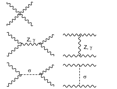
Figure 1: Gauge and $\sigma$-boson contributions to $WW\rightarrow WW$ scattering.

In the Standard Model, unitarity of the $W^{+}W^{-}\rightarrow W^{+}W^{-}$ scattering amplitude can be used to obtain a constraint on the Higgs boson mass Lee:1977eg . In the present model, the $\sigma$ field is analogous to the Standard Model Higgs boson, but its coupling to $W^{+}W^{-}$ is reduced by a factor of $f^{\prime}/v$, as we saw in Eq. (19). The Feynman diagrams involving gauge fields and the $\sigma$ boson are shown in Fig. 1. The corresponding amplitude is given at leading order by

$$\mathcal{M}_{\rm gauge}+\mathcal{M}_{\sigma}=\frac{1}{v^{2}}\left(s+t\right)-\frac{1}{v^{2}}\left(\frac{f^{\prime}}{v}\right)^{2}\left(\frac{s^{2}}{s-m_{\sigma}^{2}}+\frac{t^{2}}{t-m_{\sigma}^{2}}\right).$$ (41)

for momenta large compared to $m_{W}$. In addition, the scattering amplitude also receives important contributions from diagrams involving technirho exchanges, shown in Fig. 2. To evaluate these, we use the Goldstone boson equivalence theorem and compute the technirho-exchange contributions to $\pi_{a}^{+}\pi_{a}^{-}\rightarrow\pi_{a}^{+}\pi_{a}^{-}$, where $\pi_{a}$ is the linear combination of isotriplet fields that would be absent in unitary gauge. This will give the longitudinal $W$ boson scattering amplitude accurately for external momenta large compared to the $W$ boson mass, a criterion that will always be satisfied in the regions of parameter space that are of interest to us. The $\rho\pi_{a}\pi_{a}$ coupling is given by Eqs. (38) and (III), with $g_{\rho\Pi\Pi}$ computed holographically using Eq. (36). Thus, we find the technirho contribution to the scattering amplitude

$$\mathcal{M}_{\rho}=g_{\rho\pi_{a}\pi_{a}}^{2}\left(\frac{s+2t}{s-m_{\rho}^{2}}+\frac{2s+t}{t-m_{\rho}^{2}}\right),$$ (42)

and the total amplitude

$$\mathcal{M}=\mathcal{M}_{\rm gauge}+\mathcal{M}_{\sigma}+\mathcal{M}_{\rho}.$$ (43)

Note that the total amplitude is gauge invariant, as is $\mathcal{M}_{\rho}$ separately.

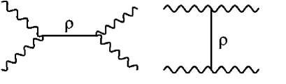
Figure 2: Technirho contributions to $WW\rightarrow WW$ scattering.

The most significant constraint from unitarity can be obtained by considering the $J=0$ partial wave

$$a_{0}(s)=\frac{1}{16\pi s}\int_{-s}^{0}\mathcal{M}\,dt.$$ (44)

Following Ref. hhg we require $|\textrm{Re }a_{0}(s)|\leq 1/2$, over the range of energies in which our holographic calculation is valid. Based on what is known from holographic models of QCD, the holographic construction is trustworthy up to the mass of the lowest vector and axial-vector resonances, but becomes increasingly less accurate when properties of heavier hadronic resonances are considered. Thus, we take the mass scale of the second vector resonance (i.e., the first excited state of the technirho) as a cutoff for our effective theory. If unitarity is violated above this scale, no conclusion can be drawn because the calculational framework is suspect. If unitarity is violated below this scale, the effective theory is excluded in its minimal form. For the $\sigma$ boson taken as light as possible, the technirho cannot be made arbitrarily heavy without violating this constraint. However, the lower bound on the technirho mass is relaxed when $f$ is made small since the model mimics the Standard Model in this limit.

IV.3 Higgs Mass

As mentioned in the previous section, the $\sigma$ field is similar to the Standard Model Higgs boson, but with modified couplings. If light enough, the $\sigma$ boson would have been produced at LEP via the Higgstrahlung process $e^{+}e^{-}\rightarrow Z^{*}\rightarrow\sigma Z$. In the region of parameter space left viable after the consideration of the unitarity and $S$ parameter bounds (discussed in the next section), the $\sigma-Z$ coupling is not less than $\sim 90$% of its Standard Model value. In this case, the LEP bound is modified in accordance with Fig. 10 of Ref. Barate:2003sz , and differs negligibly from the Standard Model result. Note that the partial decay widths to two fermions are slightly enhanced while the partial decay widths to two fermions and one gauge boson (via an off-shell gauge boson) are slightly suppressed. Hence, the branching fraction to the primary decay channels at LEP, namely $\bar{b}b$ and $\bar{\tau}\tau$, will remain practically unaffected. Thus, we will apply the bound $m_{\sigma}\geq 114.4\textrm{ GeV}$ to constrain the parameter space of the model.

The possible perturbative interactions of the $\phi$ field allow us to construct a potential for $\sigma$. Following the conventions of Ref. bt3 ,

$$V(\sigma_{s})=\frac{M^{2}}{2}\sigma_{s}^{2}+\frac{\lambda}{8}\sigma_{s}^{4}-\frac{1}{64\pi^{2}}\left[3h_{t}^{4}+2Nh^{4}\right]\sigma_{s}^{4}\ln\left(\frac{\sigma_{s}^{2}}{\mu^{2}}\right)-8\sqrt{2}\pi c_{1}f^{3}h\sigma_{s}\,,$$ (45)

where $M^{2}\geq 0$ and $\sigma_{s}=\sigma+f^{\prime}$. The third term represents the one-loop radiative corrections from the top quark and the techniquarks, though only the former is substantial. All other radiative corrections can be neglected for the values of the couplings that are relevant in the next section. In order to remove the dependence on the renormalization scale $\mu$, we define a renormalized coupling $\lambda_{r}\equiv 1/3\,V^{\prime\prime\prime\prime}(f^{\prime})$, where primes refer to derivatives with respect to $\sigma_{s}$. It is convenient for us to work with a redefined coupling $\tilde{\lambda}$, where

$$\tilde{\lambda}\equiv\lambda_{r}+\frac{11}{24\pi^{2}}\left[3h_{t}^{4}+2Nh^{4}\right]\,.$$ (46)

Since the $\sigma$ field has no vacuum expectation value, $V^{\prime}(f^{\prime})=0$, from which it follows that

$$M^{2}f^{\prime}+\frac{1}{2}\tilde{\lambda}f^{\prime 3}=8\sqrt{2}c_{1}\pi f^{3}h\,.$$ (47)

The mass of $\sigma$ is given by $V^{\prime\prime}(f^{\prime})$:

$$m_{\sigma}^{2}=M^{2}+\left(\frac{3}{2}\tilde{\lambda}-\frac{1}{8\pi^{2}}\left[3h_{t}^{4}+2Nh^{4}\right]\right)f^{\prime 2}\,.$$ (48)

We can eliminate $\tilde{\lambda}$ using Eq. (47), as well as the chiral Lagrangian parameter $c_{1}$ using Eqs. (16) and (46):

$$m_{\sigma}^{2}=3m_{\pi}^{2}\frac{f^{2}}{v^{2}}-\frac{1}{8\pi^{2}}\left[3h_{t}^{4}+2Nh^{4}\right]f^{\prime 2}-2M^{2}\,.$$ (49)

Since the last term is no smaller than zero in the models of interest, we conclude that

$$m_{\sigma}^{2}\leq 3m_{\pi}^{2}\frac{f^{2}}{v^{2}}-\frac{1}{8\pi^{2}}\left[3h_{t}^{4}+2Nh^{4}\right]f^{\prime 2}\,.$$ (50)

The physical pion mass $m_{\pi}$ is computed holographically following the discussion of Sec. III. For any region of the $f$-$m_{\rho}$ plane where the right-hand side of Eq. (50) is less than the LEP bound, the $\sigma$ mass can never be any larger, for any positive $M^{2}$.

V Numerical Results

V.1 Allowed Regions

In this subsection, we present our results for the allowed region of the model’s parameter space. We first assume $h=0.01$ and that the value of $g_{5}$ is the same as in an SU($4$) technicolor sector. For the unitarity calculation, we fix the $\sigma$ mass at the LEP bound, $114.4$ GeV; taking the $\sigma$ mass higher only makes the unitarity bound on the $\rho$ mass stronger. The excluded regions are plotted on the $f/v$ versus $m_{\rho}$ plane. We later consider how the excluded regions change as $h$ and $g_{5}$ are varied.

Our results are presented in Fig. 3. The bound from the $S$ parameter eliminates the portion of the plot with large $f$ and small technirho masses. In this region, the mass scale of the technihadrons is low and electroweak symmetry breaking is primarily a consequence of technicolor dynamics; one would expect this to correspond to a problematic value of the $S$ parameter. On the other hand, the unitarity constraint excludes the region with large $f$ and large technirho masses. Here the theory is more technicolor-like, and the technirho has a greater impact than the $\sigma$ boson in unitarizing the theory. Finally, for small values of $f$ and small technirho masses, there is no value of $M^{2}\geq 0$ for which the $\sigma$ boson mass is as large as the LEP bound. The allowed region is represented by the narrow band in the central region of Fig. 3. The intersection of the boundaries from the $S$ parameter and $\sigma$ mass bounds gives us a lower bound on the technirho mass:

$$m_{\rho}\geq 1.6\textrm{ TeV}\,,\,\,\,\,\,(h=0.01)\,.$$ (51)

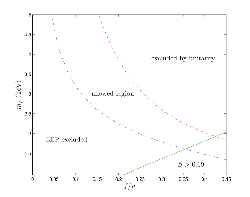
Figure 3: The allowed region for $h=0.01$.

The allowed region and the lower bound on technirho mass can change if we vary the assumed values of $h$ and $g_{5}$. In Fig. 4, we show the effect of increasing the techniquark Yukawa coupling $h$ from $0.01$ to $0.05$. While the unitarity and $S$ parameter exclusion regions are only slightly affected, the boundary of the LEP-excluded region is shifted noticeably. For a fixed point in the $f/v$-$m_{\rho}$ plane, taking $h$ larger (i.e., making the techiquarks heavier) increases the minimium possible mass of the $\sigma$ boson, by increasing the technipion mass in the first term of Eq. (50). Hence, the exclusion line shifts to lower values of the technirho mass, where $m_{\pi}$ is again reduced. A consequence of the enlarged allowed region is that the absolute lower bound on the technirho mass is relaxed:

$$m_{\rho}\geq 960\textrm{ GeV}\,,\,\,\,\,\,(h=0.05)\,.$$ (52)

One may reasonably ask what happens to the allowed parameter space as one varies $h$ further. For larger values of $h$, $m_{q}/\sigma_{c}^{1/3}$ quickly becomes of order one: the assumption of approximate chiral symmetry is lost and the predictions of the holographic theory are no longer trustworthy. If one requires $m_{q}/\sigma_{c}^{1/3}<1/3$ everywhere in the allowed region, then the largest possible techniquark Yukawa coupling is $h=0.18$, and one finds $m_{\rho}\geq 630$ GeV. On the other hand, if $h$ is taken smaller that $0.01$, the exclusion line from the LEP bound moves toward larger $m_{\rho}$, while the others do not change appreciably. For $h<1.0\times 10^{-3}$, no allowed region remains.

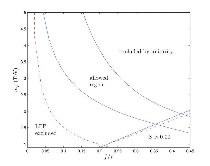
Figure 4: The allowed region as the value of $h$ is varied. The solid (dashed) lines correspond to $h=0.01$ $(0.05)$. The unitarity exclusion lines for $h=0.01$ and $h=0.05$ coincide and are represented by a single solid line.

In constructing the holographic model of the technicolor sector, the 5D gauge coupling was chosen so that current-current correlators would have the same high-$q^{2}$ behavior as in an SU($N$) gauge theory. The same approach is used in successful holographic models of QCD adsqcd , where one knows with certainty that the gauge theory of interest is SU(3). In our case, this choice simply defines the class of models that we choose to study, and allows us to make definite phenomenological predictions. While predictivity requires us to make some well-motivated choice for $g_{5}$, it is still useful study whether our predictions are sensitive to the precise value chosen. To do so, we allow $g_{5}$ to vary by half and twice the value given in Eq. (31). The results are shown in Fig. 5. One can see that the qualitative changes in the shape of the allowed region are not particularly dramatic.

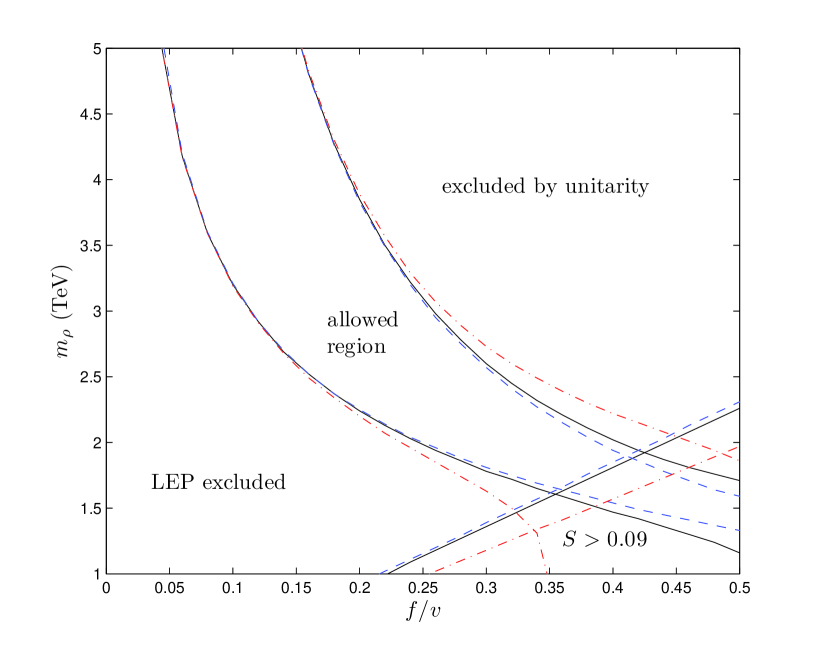
Figure 5: The allowed region as the value of $g_{5}$ is varied. The solid, dashed and dot-dashed lines correspond to $r=1$, $0.5$ and $2.0$ respectively, where $g_{5}=r\sqrt{24\pi^{2}/N}$ with $N=4$.

V.2 Technirho Decays

Since the allowed parameter space of Fig. 3 that is within the reach of the LHC is limited, it is interesting to see whether observable quantities vary appreciably within this region. We focus on the $\rho$ and technipion masses, as well as the dominant $\rho$ branching fractions. The technirho couples most strongly to the technipion field $\Pi$, which is partly $\pi_{p}$ and $\pi_{a}$. Using the fact that the technipion mass is considerably smaller than technirho mass, the decay to absorbed technipions is equal to the decay to longitudinal $W$ bosons by the Goldstone boson equivalence theorem. The interaction Lagrangian is defined in Eqs. (38) and (III), with the coupling $g_{\rho\,\Pi\,\Pi}$ calculated holographically using Eq. (36). The associated decay widths are given by cet1

$$\Gamma_{\pi_{p}\pi_{p}} = \frac{1}{48\pi}m_{\rho}g^{2}_{\rho\pi_{p}\pi_{p}}\left(1-4\frac{m_{\pi}^{2}}{m_{\rho}^{2}}\right)^{3/2},$$

$$\Gamma_{W_{L}W_{L}} = \frac{1}{48\pi}m_{\rho}g^{2}_{\rho\pi_{a}\pi_{a}}\left(1-4\frac{m_{W}^{2}}{m_{\rho}^{2}}\right)^{3/2},$$

$$\Gamma_{W_{L}^{\pm}\pi_{p}^{\mp}} = \frac{1}{48\pi}m_{\rho}g^{2}_{\rho\pi_{p}\pi_{a}}\left(1+\frac{m_{\pi}^{4}}{m_{\rho}^{4}}+\frac{m_{W}^{4}}{m_{\rho}^{4}}-2\frac{m_{W}^{2}}{m_{\rho}^{2}}-2\frac{m_{\pi}^{2}}{m_{\rho}^{2}}-2\frac{m_{\pi}^{2}m_{W}^{2}}{m_{\rho}^{4}}\right)^{3/2}.$$ (53)

There are many subleading decay modes that one could also consider. Each could be evaluated by a holographic calculation, in some cases requiring the modification of the 5D theory to include additional fields. A complete analysis goes beyond the scope of the present work. However, we will consider the decay to dileptons here, since this represents a particularly clean channel for searches at the LHC. This decay proceeds via the vector-meson dominance couplings of the technirho to the photon and the $Z$. In the 5D theory, the gauge fields of a weakly gauged subgroup of the global chiral symmetry of the boundary theory appear as coefficients of the non-normalizable modes of the bulk gauge fields ss . Substituting these into the 5D Lagrangian and integrating over the extra dimension yields the desired couplings:

$$\mathcal{L}=-\frac{m_{\rho}^{2}}{f_{\rho}}\left[eA_{\mu}+\frac{e}{2s_{\theta}c_{\theta}}(c_{\theta}^{2}-s_{\theta}^{2})Z_{\mu}\right]\rho^{\mu}\,.$$ (54)

Here $s_{\theta}$ ($c_{\theta}$) represents the sine (cosine) of the weak mixing angle. The technirho decay constant is given by

$$f_{\rho}=\frac{1}{2}\,g_{5}\,(m_{\rho}z_{m})\,J_{1}(m_{\rho}\,z_{m})\,\,.$$ (55)

Since the product $m_{\rho}\,z_{m}$ is fixed for the lowest vector resonance, one finds $f_{\rho}\approx 4.8$. The decay width to a single flavor of lepton is then straightforward to compute:

$$\Gamma_{e^{+}e^{-}} = \frac{4\pi\alpha_{EM}^{2}}{3f_{\rho}^{2}}m_{\rho}$$ (56)

$$\;\times\left[\left(Q_{e}+c_{V,e}\frac{c_{\theta}^{2}-s_{\theta}^{2}}{4s_{\theta}^{2}c_{\theta}^{2}}\frac{m_{\rho}^{2}}{m_{\rho}^{2}-m_{Z}^{2}}\right)^{2}+\left(c_{A,e}\frac{c_{\theta}^{2}-s_{\theta}^{2}}{4s_{\theta}^{2}c_{\theta}^{2}}\frac{m_{\rho}^{2}}{m_{\rho}^{2}-m_{Z}^{2}}\right)^{2}\right].$$

Here $Q_{e}=-1$, $c_{V,e}=-1/2+2s_{\theta}^{2}$, and $c_{A,e}=-1/2$. The total decay width is obtained by summing the partial widths for all decay channels. Ignoring some of the possible subleading modes only provides small corrections to the branching fractions that we consider here.

No.	$m_{\rho}$ (TeV)	$f/v$	$m_{\pi}/m_{\rho}$	$\Gamma_{\rho}/m_{\rho}$	$\textrm{BR}_{WW}$ (%)	$\textrm{BR}_{W\pi}$ (%)	$\textrm{BR}_{\pi\pi}$ (%)	$\textrm{BR}_{e^{+}e^{-}}$ (%)
1	1.59	0.36	0.13	0.23	1.8	23.3	74.9	$5\times 10^{-3}$
2	1.90	0.36	0.12	0.24	1.8	23.3	74.9	$5\times 10^{-3}$
3	2.21	0.36	0.12	0.24	1.8	23.3	74.8	$5\times 10^{-3}$
4	2.21	0.29	0.13	0.25	0.78	16.1	83.1	$5\times 10^{-3}$
5	2.21	0.22	0.15	0.24	0.27	9.8	89.9	$5\times 10^{-3}$
6	2.90	0.22	0.15	0.24	0.27	9.8	89.8	$5\times 10^{-3}$
7	3.50	0.22	0.15	0.25	0.27	9.8	89.8	$5\times 10^{-3}$
8	3.50	0.16	0.18	0.23	0.08	5.5	94.4	$5\times 10^{-3}$
9	3.50	0.11	0.22	0.20	0.01	2.4	97.6	$6\times 10^{-3}$
10	5.00	0.15	0.18	0.23	0.06	4.9	95.0	$5\times 10^{-3}$
11	5.00	0.10	0.22	0.21	0.01	2.4	97.6	$6\times 10^{-3}$
12	5.00	0.05	0.31	0.14	$0.001$	0.76	99.1	$8\times 10^{-3}$

Table 1: Technirho decay table for $h=0.01$

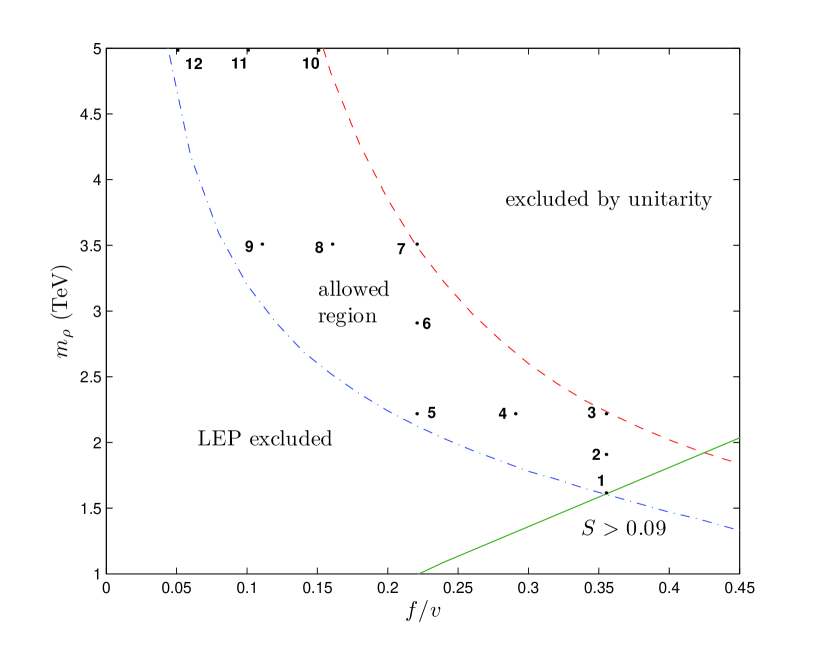
Figure 6: Twelve sample points considered in Table 1. The allowed region assumes $h=0.01$.

Table 1 presents our results for the case $h=0.01$, over a set of sample points within the allowed region of the model’s parameter space. The location of the sample points is shown in Fig. 6. From the table, we see that the total decay width depends almost solely on $m_{\rho}$ for $m_{\rho}<5$ TeV (we don’t consider larger masses, which are not likely to be within the reach of the LHC). The branching fractions, on the other hand, depend mostly on $f/v$. As $f/v$ becomes smaller, the branching fraction of the technirho to two physical pions increases, since the other dominant decay channels, $W_{L}\pi$ and $W_{L}W_{L}$, are suppressed by factors of $f/v$ and $f^{2}/v^{2}$, respectively. Everywhere in the allowed parameter space the decay mode to $\pi_{p}\pi_{p}$ is dominant. The branching fraction to dileptons varies only between $5\times 10^{-5}$ and $8\times 10^{-5}$, always significantly suppressed compared to the leading modes. We have estimated that detection of the technirho via its decays to dileptons at the LHC would be feasible only if the dominant modes to technipions were kinematically forbidden. However, this favorable situation only occurs in regions of parameter space that are excluded by the bounds we have considered.

VI Conclusions

We have shown how the combined constraints from the $S$ parameter, partial-wave unitarity and searches for a light Higgs-like scalar, meaningfully limit the viable parameter space of a simple holographic bosonic technicolor model. The parameter space of the model itself indicates an important difference between this model and conventional, QCD-like technicolor theories: different points in the $f$-$m_{\rho}$ plane have different ratios of the chiral symmetry breaking scale to the confinement scale. In QCD-like technicolor, this ratio is fixed. The $S$ parameter eliminates the region where $f$ is large and $m_{\rho}$ is small. Here, technicolor dynamics is the primary agent responsible for electroweak symmetry breaking. Perturbative unitarity eliminates the region where $f$ is large and $m_{\rho}$ is large. Here, the technirho is more important than the Higgs-like scalar in unitarizing the theory. Finally, the LEP bound on the mass of the Higgs-like scale eliminates the region where both $m_{\rho}$ and $f$ are small. Below $m_{\rho}<5$ TeV, a limited region of allowed parameter space remains. We pointed out a number of physical quantities (for example, the ratio of the physical pion to technirho mass and the technirho branching fraction to two pions) that do not vary strongly within this region. We also studied how the allowed region changes as the techniquark mass and the 5D gauge coupling are varied.

In the near future, data from the LHC may make it possible to rule out this type of model, without recourse to philosophical or aesthetic arguments. For example, something as simple as a tighter lower bound on the neutral scalar mass could substantially squeeze or eliminate the allowed band in Fig. 3. As another example, we have found that within the allowed region, the branching fraction of the technirho to two physical pions varies between 75-100%, suggesting a channel for future collider studies. Other decay modes that we have not considered may be of value in excluding additional parameter space, but these require additional holographic analysis as well as dedicated collider studies.

- (1) S. Weinberg, Phys. Rev. D 19, 1277 (1979); E. Farhi and L. Susskind, Phys. Rev. D 20, 3404 (1979).
- (2) M. E. Peskin and T. Takeuchi, Phys. Rev. Lett. 65, 964 (1990); M. E. Peskin and T. Takeuchi, Phys. Rev. D 46, 381 (1992).
- (3) S. Dimopoulos and L. Susskind, Nucl. Phys. B 155, 237 (1979).
- (4) D. K. Hong and H. U. Yee, Phys. Rev. D 74, 015011 (2006) [arXiv:hep-ph/0602177].
- (5) J. Hirn and V. Sanz, Phys. Rev. Lett. 97, 121803 (2006) [arXiv:hep-ph/0606086].
- (6) C. D. Carone, J. Erlich and J. A. Tan, Phys. Rev. D 75, 075005 (2007) [arXiv:hep-ph/0612242].
- (7) K. Agashe, C. Csaki, C. Grojean and M. Reece, JHEP 0712, 003 (2007) [arXiv:0704.1821 [hep-ph]].
- (8) C. D. Carone, J. Erlich and M. Sher, Phys. Rev. D 76, 015015 (2007) [arXiv:0704.3084 [hep-th]].
- (9) T. Hirayama and K. Yoshioka, JHEP 0710, 002 (2007) [arXiv:0705.3533 [hep-ph]].
- (10) K. Haba, S. Matsuzaki and K. Yamawaki, Prog. Theor. Phys. 120, 691 (2008) [arXiv:0804.3668 [hep-ph]].
- (11) M. Fabbrichesi, M. Piai and L. Vecchi, Phys. Rev. D 78, 045009 (2008) [arXiv:0804.0124 [hep-ph]].
- (12) D. D. Dietrich and C. Kouvaris, Phys. Rev. D 78, 055005 (2008) [arXiv:0805.1503 [hep-ph]]; Phys. Rev. D 79, 075004 (2009) [arXiv:0809.1324 [hep-ph]]; D. D. Dietrich, M. Jarvinen and C. Kouvaris, arXiv:0908.4357 [hep-ph].
- (13) O. Mintakevich and J. Sonnenschein, JHEP 0907, 032 (2009) [arXiv:0905.3284 [hep-th]].
- (14) N. Kitazawa, arXiv:0908.2663 [hep-th].
- (15) M. Round, arXiv:1003.2933 [hep-ph].
- (16) A. V. Belitsky, arXiv:1003.0062 [hep-ph].
- (17) M. Antola, S. Di Chiara, F. Sannino and K. Tuominen, arXiv:1001.2040 [hep-ph]; M. Jarvinen and F. Sannino, arXiv:0911.2462 [hep-ph]; F. Sannino, arXiv:0911.0931 [hep-ph].
- (18) J. A. Evans, J. Galloway, M. A. Luty and R. A. Tacchi, arXiv:1001.1361 [hep-ph].
- (19) See also, K. Kainulainen, K. Tuominen and J. Virkajarvi, arXiv:1001.4936 [astro-ph.CO].
- (20) J. M. Maldacena, Adv. Theor. Math. Phys. 2, 231 (1998) [Int. J. Theor. Phys. 38, 1113 (1999)] [arXiv:hep-th/9711200]; S. S. Gubser, I. R. Klebanov and A. M. Polyakov, Phys. Lett. B 428, 105 (1998) [arXiv:hep-th/9802109]; E. Witten, Adv. Theor. Math. Phys. 2, 253 (1998) [arXiv:hep-th/9802150].
- (21) J. Erlich, E. Katz, D. T. Son and M. A. Stephanov, Phys. Rev. Lett. 95, 261602 (2005) [arXiv:hep-ph/0501128]; L. Da Rold and A. Pomarol, Nucl. Phys. B 721, 79 (2005) [arXiv:hep-ph/0501218].
- (22) J. Erlich and C. Westenberger, Phys. Rev. D 79, 066014 (2009) [arXiv:0812.5105 [hep-ph]].
- (23) R. S. Chivukula, A. G. Cohen and K. D. Lane, Nucl. Phys. B 343, 554 (1990).
- (24) A. Kagan and S. Samuel, Phys. Lett. B 252, 605 (1990); Phys. Lett. B 270, 37 (1991); Phys. Lett. B 284, 289 (1992).
- (25) E. H. Simmons, Nucl. Phys. B 312, 253 (1989).
- (26) C. D. Carone and H. Georgi, Phys. Rev. D 49, 1427 (1994) [arXiv:hep-ph/9308205].
- (27) C. D. Carone and E. H. Simmons, Nucl. Phys. B 397, 591 (1993) [arXiv:hep-ph/9207273].
- (28) C. D. Carone and M. Golden, Phys. Rev. D 49, 6211 (1994) [arXiv:hep-ph/9312303].
- (29) C. D. Carone, E. H. Simmons and Y. Su, Phys. Lett. B 344, 287 (1995) [arXiv:hep-ph/9410242].
- (30) V. Hemmige and E. H. Simmons, Phys. Lett. B 518, 72 (2001) [arXiv:hep-ph/0107117].
- (31) C. X. Yue, Y. P. Kuang, G. R. Lu and L. D. Wan, Mod. Phys. Lett. A 11, 289 (1996); X. L. Wang, B. Huang, G. R. Lu, Y. D. Yang and H. B. Li, Commun. Theor. Phys. 27, 325 (1997); Y. G. Cao and Z. K. Jiao, Commun. Theor. Phys. 38, 47 (2002).
- (32) M. Antola, M. Heikinheimo, F. Sannino and K. Tuominen, arXiv:0910.3681 [hep-ph].
- (33) A. Manohar and H. Georgi, Nucl. Phys. B 234, 189 (1984); H. Georgi and L. Randall, Nucl. Phys. B 276, 241 (1986).
- (34) C. Amsler et al. [Particle Data Group], Phys. Lett. B 667, 1 (2008).
- (35) K. Agashe, R. Contino and A. Pomarol, Nucl. Phys. B 719, 165 (2005) [arXiv:hep-ph/0412089].
- (36) B. W. Lee, C. Quigg and H. B. Thacker, Phys. Rev. D 16, 1519 (1977).
- (37) J. F. Gunion, H. E. Haber, G. L. Kane and S. Dawson, “The Higgs Hunter’s Guide,” Redwood City, California: Addison-Wesley (1990) 404p.
- (38) R. Barate et al. [LEP Working Group for Higgs boson searches and ALEPH Collaboration and and], Phys. Lett. B 565, 61 (2003) [arXiv:hep-ex/0306033].
- (39) T. Sakai and S. Sugimoto, Prog. Theor. Phys. 114, 1083 (2005) [arXiv:hep-th/0507073].