Pressure Solution in Sedimentary Basins:
Effect of Temperature Gradient

Abstract

Pressure solution is an important process in sedimentary basins, and its behaviour depends mainly on the sediment rheology and temperature distribution. The compaction relation of pressure solution is typically assumed to be a viscous one and is often written as a relationship between effective stress and strain rate. A new derivation of viscous compaction relation is formulated based on more realistic boundary conditions at grain contacts. A nonlinear diffusion problem with a moving boundary is solved numerically and a simple asymptotic solution is given to compare with numerical simulations. Pressure solution is significantly influenced by the temperature gradient. Porosity reduction due to pressure solution is enhanced in an environment with a higher thermal gradient, while porosity decreases much slowly in the region where the thermal gradient is small. Pressure solution tends to complete more quickly at shallower depths and earlier time in higher temperature environment than that in a low one. These features of pressure solution in porous sediments are analysed using a perturbation method to get a solution for the steady state. Comparison with real data shows a reasonably very good agreement.

Key Words: viscous compaction, pressure solution, asymptotic analysis, temperature gradient.

Citation detail: X. S. Yang, Pressure solution in sedimentary basins: effect of temperature gradient, Earth and Planetary Science Letters, 176, 233-243 (2000).

1 INTRODUCTION

Pressure solution is a very common and important deformation process in porous media and granular materials such as sediments and soils. Pressure solution also occurs in sedimentary basins where hydrocarbons and oil are primarily formed. The modelling of such compactional flow is thus important in the oil industry as well as in civil engineering. One particular problem which affects drilling process is the occasional occurrence of abnormally high pore fluid pressures, which, if encountered suddenly, can cause drill hole collapse and consequent failure of the drilling operation. Therefore, an industrially important objective is to predict overpressuring before drilling and to identify its precursors during drilling. An essential step to achieve such objectives is the scientific understanding of their mechanisms and the evolutionary history of post-depositional sediments such as shales.

Compaction is the process of volume reduction via pore-water expulsion within sediments due to the increasing weight of overburden load. The requirement of its occurrence is not only the application of an overburden load but also the expulsion of pore water. The extent of compaction is strongly influenced by sedimentation history and the lithology of sediments. The freshly deposited loosely packed sediments tend to evolve, like an open system, towards a closely packed grain framework during the initial stages of burial compaction and this is accomplished by the processes of grain slippage, rotation, bending and brittle fracturing. Such reorientation processes are collectively referred to as mechanical compaction, which generally takes place in the first 1 - 2 km of burial. After this initial porosity loss, further porosity reduction is accomplished by the process of chemical compaction such as pressure solution at grain contacts [1,2,3].

Pressure solution has been considered as an important process in deformation and porosity change during compaction in sedimentary rocks [4,5]. Pressure solution refers to a process by which grains dissolve at intergranular contacts under non-hydrostatic stress and reprecipitate in pore spaces, thus resulting in compaction. The solubility of minerals increases with increasing effective stress at grain contacts. Pressure dissolution at grain contacts is therefore a compactional response of the sediment during burial in an attempt to increase the grain contact area so as to distribute the effective stress over a larger surface. Such a compaction process is typically assumed to viscous [5,6,7] and it is usually referred to as viscous compaction, viscous creep or pressure solution creep. Its rheological constitutive relation (or compaction relation) is often written as a relationship between effective stress and strain rate.

A typical form of pressure solution is intergranular pressure solution (IPS) which occurs at individual grain contacts and free face pressure solution (FFPS) which occurs at the face in contact with the pore fluid, but most studies have concentrated on the former one (IPS). Extensive studies [1,5,6,7,8] on pressure solutin have been carried out in the last two decades, and a comprehensive literature review on these models was given by Tada and Siever [8]. A more recent and brief review can be found in [5,6]. Despite of its geological importance, the mechanism of pressure solution is still poorly understood. Recently, Fowler and Yang [5] present a new mathematical approach to model pressure solution and viscous compaction in sedimentary basins and show that the main parameter controlling the compaction and porosity reduction is the compaction parameter $\lambda$, the ratio of hydraulic conductivity to the sedimentation rate. Compaction relation of poro-elastic and viscous type is also an important factor controlling the behaviour of compaction profile. However, the temperature effect has not been included in their approach. Thus, we mainly investigate the effect of different temperature gradients on the viscous compaction due to pressure solution in sedimentary basins.

2 MATHEMATICAL MODEL

For the convenience of investigating the effect of compaction in porous media due to pure density differences, we will assume the basic model of compaction is rather analogous to the process of soil consolidation. The porous media act as a compressible porous matrix, so that mass conservation of pore fluid together with Darcy’s law leads to the 1-D model equations of the general type [1,5].

$$\frac{\partial\rho_{s}(1-\phi)}{\partial t}+\frac{\partial}{\partial z}[\rho_{s}(1-\phi)u^{s}]=0,\,\,\,\,({\rm solid\,\,phase})$$ (1)

$$\frac{\partial\rho_{l}\phi}{\partial t}+\frac{\partial(\rho_{l}\phi u^{l})}{\partial z}=0,\,\,\,\,({\rm liquid\,\,phase})$$ (2)

$$\phi(u^{l}-u^{s})=-\frac{k(\phi)}{\mu}[\frac{\partial p}{\partial z}+\rho_{l}g],\,\,\,\,({\rm Darcy^{\prime}s\,\,law})$$ (3)

$$-\frac{\partial}{\partial z}[(1+\frac{4\eta}{3\xi})p_{e}]-\frac{\partial p}{\partial z}-[\rho_{s}(1-\phi)+\rho_{l}\phi]g=0,$$

$$({\rm force\,\,balance}),$$ (4)

where $u^{l}$ and $u^{s}$ are the velocities of fluid and solid matrix, $k$ and $\mu$ are the matrix permeability and the liquid viscosity, $\rho_{l}$ and $\rho_{s}$ are the densities of fluid and solid matrix, $p$ is pore pressure, $p_{e}$ is the effective pressure, $\eta$ is medium viscosity and $\xi$ is compaction viscosity, and $g$ is the gravitational acceleration. Combining the force balance and Darcy’s law to eliminate $p$, we have

$$\phi(u^{l}-u^{s})=\frac{k(\phi)}{\mu}\{\frac{\partial}{\partial z}[(1+\frac{4\eta}{3\xi})p_{e}]-(\rho_{s}-\rho_{l})(1-\phi)g\},$$ (5)

which is a derived form of Darcy’s law. By assuming the densities $\rho_{s}$ and $\rho_{l}$ are constants, we can see that only the density difference $\rho_{s}-\rho_{l}$ is important to the flow evolution. Thus, the compactional flow is essentially density-driven flow in porous media.

Compaction relation is a relationship between effective pressure $p_{e}$ and strain rate $\dot{e}=\frac{\partial u^{s}}{\partial z}$ or porosity $\phi$ [5,6,7]. The common approach in soil mechanics and sediment compaction is to model this generally nonlinear behaviour as poroelastic, that is to say, a relationship of Athy’s law type $p_{e}=p_{e}(\phi)$, which is derived from fitting the real data of sediments. However, this poroelastic compaction law is only valid for the compaction in porous media in the upper and shallow region, where compaction occurs due to the pure mechanical movements such as grain sliding and packing rearrangement. In the more deeper region, mechanical compaction is gradually replaced by the chemical compaction due to stress-enhanced flow along the grain boundary from the grain contact areas to the free pore, where pressure is essentially pore pressure. A typical process of such chemical compaction in sediment is pressure solution whose rheological behavior is usually viscous, so that it sometimes called viscous pressure solution.

The mathematical formulation for viscous compaction is to derive a relation between creep rate $\dot{e}$ and effective stress $\sigma_{e}$. Rutter’s creep relation is widely used [7,8,9]

$$\dot{e}=\frac{A_{k}c_{0}\,wD_{gb}}{\rho_{s}\bar{d}^{3}}\sigma_{e},$$ (6)

where $\sigma_{e}$ is the effective normal stress across the grain contacts, $A_{k}$ is a constant, $c_{0}$ is the equilibrium concentration (of quartz) in pore fluid, $\rho,\,\bar{d}$ are the density and (averaged) grain diameter (of quartz). $D_{gb}$ is the diffusivity of the solute in water along grain boundaries with a thickness $w$. $D_{gb}$ also varies with temperature $T$

$$D_{gb}(T)=D_{gb}e^{-\frac{E_{a}}{RT}},$$ (7)

where $E_{a}$ is the effective activation energy with a value of $3\sim 6$ kJ/mole or even much lower [1, 6]. From the values of the diffusion coefficient in quartz-water and rocksalt-water systems at $300,\,600,1200$ K, we get an estimate value of $E_{a}\approx 0.65$ kcal/mole [1,7].

Note that $\sigma_{e}=-(1+\frac{4\eta}{3\xi})p_{e}$ and $\dot{e}=\frac{\partial u^{s}}{\partial z}$. With this, (6) becomes the following compaction law

$$p_{e}=-\xi\nabla.{\bf u}^{s}.$$ (8)

More generally speaking, $\xi$ is also a function of porosity $\phi$. The compaction law is analogous to Fowler’s viscous compaction laws used in studies of magma transport in the Earth’s mantle.

2.1 Derivation of Viscous Law

The approach of deriving the law of viscous compaction depends on the underlying mechanism. The classical theoretical consideration assumed a grain-boundary diffusion film of constant thickness and diffusivity, while others used the concept of a roughened, fluid-invaded non-equilibrium contact structure Shimizu [6] presented a kinetic approach extending Coble’s classical treatment of grain boundary diffusion creep by including the kinetics of quartz dissolution/precipitation reaction. Shimuzu’s derivation is instructive although the boundary conditions used in his formulation are questionable and unrealistic. In addition, Shimuzu’s 1-D approximation is only valid for a closed system due to $\frac{\partial c}{\partial x}=0$ used in his work when the thickness $w$ of the water film is small with respect to the grain diameter ($\bar{d}$) [5,10]. In order to correctly formulate the derivation, we now provide a new derivation by using more realistic boundary conditions in an open system.

Now let us consider the intergranular contact region as a disk with a radius $r=L$. Let $J(r)$ be the radial component of solute mass flux, $\dot{e}$ be the average strain rate, and $v$ is the uniform shortening velocity of the upper grain relative to the lower grain due to the pressure solution creep [6,10]. The kinetic relation between $v$ and $\dot{e}$ becomes

$$v=\dot{e}\bar{d}.$$ (9)

For simplicity, we assume that the film thickness $w$ is constant and the diffusion is near steady-state. Mass conservation gives

$$2\pi rJ(r)+\rho_{s}\pi r^{2}v=0,$$ (10)

where the flux $J(r)$ obeys Fick’s Law

$$J(r)=-D_{gb}w\frac{dc}{dr}.$$ (11)

The steady-state solution of concentration $c(r)$ for the boundary conditions $c_{r}=0$ at $r=0$, $c=c_{0}$ at $r=L$ is

$$c(r)=c_{0}-\frac{\rho_{s}v}{4D_{gb}w}(L^{2}-r^{2}).$$ (12)

The parabolic change of concentration $c(r)$ implies that the stress $\sigma(r)$ should be heterogeneously distributed in the contact region. From a relation of effective stress and concentration [10], we have

$$\sigma^{e}(r)=-\frac{RT}{\nu_{m}}{\rm ln}\frac{c(r)}{c_{0}},$$ (13)

where $\nu_{m}$ is the molar volume of the sediment. We have used here the condition $\sigma^{e}(r)=0$ at $r=L$. Let $\sigma$ be the averaged effective stress, then

$$\pi L^{2}\sigma=\int^{L}_{0}2\pi\sigma^{e}(r)rdr.$$ (14)

Combining (13) and (14), we have

$$\sigma=-\frac{2RT}{\nu_{m}L^{2}}\int^{L}_{0}r{\rm ln}[1-\frac{\rho_{s}\dot{e}\bar{d}}{4c_{0}D_{gb}w}(L^{2}-r^{2})]dr.$$ (15)

Using (9) and integrating by parts, we have

$$\sigma=-\frac{RT}{\nu_{m}}[(1-\frac{1}{BL^{2}}){\rm ln}(1-BL^{2})-1],$$ (16)

where

$$B=\frac{\rho_{s}\dot{e}\bar{d}}{4c_{0}D_{gb}w}.$$ (17)

By defining a critical effective stress $\sigma_{c}$ (and equivalently a critical creep rate $\dot{e}_{c}$ ) when $BL^{2}=1$

$$\sigma_{c}\equiv\frac{RT}{\nu_{m}},\,\,\,\,\,\dot{e}_{c}\equiv\frac{4c_{0}D_{gb}w}{\rho_{s}L^{2}\bar{d}},$$ (18)

equation (16) can be rewritten as

$$\frac{\sigma}{\sigma_{c}}=[1-(1-\frac{\dot{e}_{c}}{\dot{e}})\ln(1-\frac{\dot{e}}{\dot{e}_{c}})].$$ (19)

From the typical values of $T\sim 300$ K, $R\sim 8.31$ J mol^-1 K^-1, and $\nu_{m}\sim 2.6\times 10^{-5}$ m³ mol^-1 [11], we can use the definition (18) to estimate the typical value of $\sigma_{c}$, which is about $95$ MPa. Clearly, if $\mid\!\sigma\!\mid\,\ll\sigma_{c}$, we have

$$\dot{e}=\frac{4\nu_{m}c_{0}D_{gb}w}{RT\rho_{s}\bar{d}L^{2}}\sigma=\frac{16\nu_{m}c_{0}D_{gb}w}{RT\rho_{s}\bar{d}^{3}}\sigma,$$ (20)

which is exactly the creep law. Here we have used $L=\bar{d}/2$. A different choice of $L=O(\bar{d})$ will only introduce an additional shape factor into the above relation. Under upper-crustal stress conditions $\sigma<100$ MPa, the above approximation is valid as we expected. At higher stress states, we can use $\mid\!\sigma\!\mid\,\gg\sigma_{c}$, then (19) becomes

$$\dot{e}=\frac{4c_{0}D_{gb}w}{\rho_{s}\bar{d}L^{2}}[1-e^{-\frac{\nu_{m}\sigma}{RT}}].$$ (21)

Let $L^{2}=4\bar{d}^{2}/\alpha_{s}$, and $\alpha_{s}=O(1)$ is a shape factor. The above relation (21) becomes

$$\dot{e}=\frac{\alpha_{s}c_{0}D_{gb}w}{\rho_{s}\bar{d}^{3}}[1-e^{-\frac{\nu_{m}\sigma}{RT}}],$$ (22)

which degenerates into (20) when $\nu_{m}\sigma/RT\ll 1$, but (20) may be inaccurate when $\mid\!\sigma\!\mid\,\sim\sigma_{c}$. The new compaction relation (22) is more accurate and valid in a more wide range of parameter variations.

Furthermore, the newly derived viscous compaction law (22) shows that the strain rate due to pressure solution is controlled by many parameters such as grain size ($\bar{d}$), grain geometry ($\alpha_{s}$), temperature ($T$), grain-boundary diffusion coeffient ($D_{gb}$). This is consistent with Dewers and Hajash’s [12] empirical law derived from a quartz compaction experiment. However, since the complicated dependence on many parameters and nonlinear features in (22), various simplified version or approximate forms have been used by many authors in earlier work [13-16]. One common simplification of (22) is its linearised form such as (6) used by Rutter [7] and Ortoleva [13]. A slightly different formulation of this compaction law is expressed in terms of porosity strain versus effective stress (instead of using the strain rate). Schneider et al. [14] used a relationship between porosity and effective stress while Lander and Walderhaug [15] used an exponential form of intergranular volume as a function of effective stress. Revil [16] used a relationship between porosity strain and effective stress, which includes time $t$ explicitly in his formulation. However, these different formulations can be transformed into a relationship similar to (20) but such a transformation may depend on the grain packing structure because of the calculation of porosity strain and porosity. For simplicity, we will only use the form (20) in the rest of the paper.

2.2 Boundary conditions

The boundary conditions for the governing equations are as follows. The bottom boundary at $z=0$ is assumed to be impermeable

$$u^{s}=u^{l}=0,$$ (23)

and a top condition at $z=h$ is kinetic

$$\dot{h}=\dot{m}_{s}+u^{s},$$ (24)

where $\dot{m}_{s}$ is the sedimentation rate at $z=h$. Also at $z=h$,

$$\phi=\phi_{0},\,\,\,\,p_{e}=p_{0},$$ (25)

where $p_{0}$ is the applied effective pressure at the top of the porous media, and $\phi_{0}$ is the initial porosity.

3 Non-dimensionalization

If a length-scale $d$ is a typical length [9] defined by

$$d=\{\frac{\xi\dot{m}_{s}G}{(\rho_{s}-\rho_{l})g}\}^{\frac{1}{2}},\,\,\,\,G=1+\frac{4\eta_{0}}{3\xi_{0}},$$ (26)

and the effective pressure is scaled in the following way

$$p=\frac{G(p_{e}-p_{0})}{(\rho_{s}-\rho_{l})gd},$$ (27)

so that $p=O(1)$. Here $G=1+\frac{4\eta_{0}}{3\xi_{0}}$ is the value at the basin top. Compaction viscosity $\xi$ varies slowly with temperature as shown below in equation (32) where $\beta\ll 1$ and $\kappa\ll 1$, and the medium viscosity $\eta$ also varies slowly with temperature so that the factor $\frac{4\eta}{3\xi}$ does not change significantly because the variations of these two viscosities may cancel in some way as we now mainly focus on the region where temperature is relative low ($<400$ K). Therefore, for simplicity, we take $G$ to be constant. Meanwhile, we scale $z$ with $d$, $u^{s}$ with ${\dot{m}}_{s}$, time $t$ with $d/{\dot{m}}_{s}$, permeability $k$ with $k_{0}$, and write

$$T=T_{0}+\frac{\gamma d}{T_{0}}\Theta,$$ (28)

where $\gamma$ is the thermal gradient, and $T_{0}$ is the temperature at the basin top. we thus have

$$-\frac{\partial\phi}{\partial t}+\frac{\partial}{\partial z}[(1-\phi)u^{s}]=0,$$ (29)

$$\frac{\partial\phi}{\partial t}+\frac{\partial(\phi u^{l})}{\partial z}=0,$$ (30)

$$\phi(u^{l}-u^{s})=\lambda k(\phi)[\frac{\partial p}{\partial z}-(1-\phi)].$$ (31)

The viscous relation becomes

$$p=-(1+\beta\Theta)e^{-\kappa\Theta}\frac{\partial u^{s}}{\partial z}.$$ (32)

where

$$\lambda=\frac{k_{0}(\rho_{s}-\rho_{l})g}{\mu{\dot{m}}_{s}},\,\,\,\,\beta=\frac{\gamma d}{T_{0}},\,\,\,\,\kappa=\frac{E_{a}\gamma d}{RT^{2}_{0}}.$$ (33)

Adding (29) and (30) together and integrating from the bottom, we have

$$u^{s}=-\phi(u^{l}-u^{s})=-u,$$ (34)

where $u=\phi(u^{l}-u^{s})$ is the Darcy flow velocity. Now we have

$$\frac{\partial\phi}{\partial t}+\frac{\partial}{\partial z}[(1-\phi)u]=0,$$ (35)

$$u=-\lambda k(\phi)[\frac{\partial p}{\partial z}-(1-\phi)].$$ (36)

The constitutive relation for permeability $k(\phi)$ is nonlinear and complicated depending on many parameters such as grain geometry, grain size distribution, materials and even the sedimentary history. For simplicity without losing the essence of physical mechanism of pressure solution concerned here, we use a simpler form

$$k(\phi)=(\frac{\phi}{\phi_{0}})^{m},$$ (37)

where the exponent $m$ is derived from experimental studies. Recently, Pape et al. [17] suggested that $m=1\sim 10$ based on fractal modelling on permeability and extensive experimental studies for 640 core samples. Considering earlier investigations [2,4,5,17], we here choose a relative high value, say, $m=8$, which is a typical value for shaly sediments.

Different relationship of $p$ and $\phi$ or $u$ leads to different compaction model equations, and thus we have

$$\frac{\partial\phi}{\partial t}=\lambda\frac{\partial}{\partial z}\{(1-\phi)(\frac{\phi}{\phi_{0}})^{m}[\frac{\partial p}{\partial z}-(1-\phi)]\},$$ (38)

$$p=\lambda(1+\beta\Theta)e^{-\kappa\Theta}\frac{\partial}{\partial z}\{(\frac{\phi}{\phi_{0}})^{m}[\frac{\partial p}{\partial z}-(1-\phi)]\},$$ (39)

The boundary conditions are

$$\frac{\partial p}{\partial z}-(1-\phi)=0,\,\,\,\,{\rm at}\,\,\,\,z=0,$$ (40)

$$\phi=\phi_{0},\,\,\,\,\dot{h}=\dot{m}(t)+\lambda(\frac{\phi}{\phi_{0}})^{m}[\frac{\partial p}{\partial z}-(1-\phi)]\,\,\,\,\,\,{\rm at}\,\,\,\,z=h(t).$$ (41)

where $\dot{m}(t)=O(1)$ is a prescribed function of time, which can be taken to be one for constant sedimentation on top of the porous media. Obviously, $\dot{m}=0$ if there is no further sedimentation and no increasing loading on top of the porous media.

For simplicity, we can use a prescribed linear temperature profile

$$\Theta=h(t)-z.$$ (42)

It is useful for the understanding of the solutions to get an estimate for $\lambda$ by using values taken from observations [6,7,9]. By using the typical values of $\rho_{l}\sim 10^{3}\,{\rm kg\,m}^{-3},\,\rho_{s}\sim 2.5\times 10^{3}\,{\rm kg\,m}^{-3},\,$ $k_{0}\sim 10^{-15}-\!\!-10^{-20}\,{\rm m}^{2},\,\mu\sim 10^{-3}\,{\rm N\,s\,m}^{2},\,\xi\sim 1\times 10^{21}$ N s ${\rm m}^{-2},$ $\dot{m}_{s}\sim 300\,{\rm m\,\,Ma}^{-1}=1\times 10^{-11}\,{\rm m\,\,s}^{-1},\,g\approx 10{\rm m\,s}^{-2},\,G\approx 1,\,E_{a}\sim 3\,{\rm kcal\,mol}^{-1},\,$ and $\gamma=0.03\,{\rm K\,m}^{-1}$ =(30 K/1000 m); then $\lambda\approx 0.01-\!-1000$, $\beta\approx 0.1$, $\kappa\approx 0.2$ and $d\approx 1000$ m.

4 Numerical Simulations and Asymptotic Analysis

4.1 Numerical Results

The nonlinear diffusion equations have been solved by using an implicit predictor-corrector method. A normalized grid parameterized is used to get a rescaled height variable $Z=z/h(t)$ in a fixed domain, which will make it easy to compare the results of different times with different values of dimensionless parameters in a fixed frame. This transformation maps the basement of the basin to $Z=0$ and the basin top to $Z=1$. The calculations were mainly implemented for the time evolutions in the range of $t=0.5\sim 10$ since the thickness in the range of $0.5{\rm km}\sim 10{\rm km}$ is the one of interest in the petroleum industry and in civil engineering. Numerical results are briefly presented and explained below. The comparison with the asymptotic solutions for equilibrium state will be made in the next section.

The compaction parameter $\lambda\approx 0.01-\!-1000$, which is the ratio between the permeability and the sedimentation rate, defines a transition between the slow compaction ($\lambda<<1$) and fast compaction ($\lambda>>1$). As shown in [5], slow compaction is the compaction in a boundary layer near the basin bottom, and $\phi\approx\phi_{0}=0.5$, while the more interesting case is the fast compaction where porosity $\phi$ reduce quickly. However, the effect of temperature gradient is not included there. Therefore, we now mainly investigate the effect of temperature gradient in the case of fast compaction when $\lambda\gg 1$.

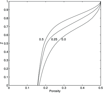
Figure 1: Viscous compaction profile of porosity versus the rescaled height $Z=z/h(t)$ at different temperature gradient $\bar{\beta}=0.05,0.25,0.5$ for $\lambda=100$ and $t=10$. The profile now is nearly parabolic.

Figure 1 provides the viscous compaction profile of porosity versus the rescaled height $Z=z/h(t)$ at different temperature gradient $\bar{\beta}=0.05,0.25,0.5$ for $\lambda=100$ and $t=10$. We can see that viscous compaction profile is more or less parabolic in the top region. Temperature gradient greatly influence the compaction behavior as pressure solution proceed, but the thermal effect is only of secondary importance, which is consistent with previous results [1]. Compared with the case of constant permeability, porosity decreases much slower in the present case and this in fact implies the increase of the pore pressure. As the depth increases, the permeability $k(\phi)=(\phi/\phi_{0})^{m}$ may become very small as $\phi<\phi_{0}$ for a relative high value of $m$, which will in turn constrain the flow through the porous media, and consequently the pore fluid in sediments gets trapped in the lower permeability zone, resulting the sudden increase of high pore pressure. This can explain the general occurrance of the high pore pressure in sedimentary basins.

Figure 2 gives the basin thickness $h(t)$ as a function of time $t$ for different values of $\lambda=0.1,10,1000$. It clearly show that the moving boundary $z=h(t)$ increases almost linearly with time $t$, which implies that $\dot{h}=const$, but $\dot{h}$ is a function of compaction parameter $\lambda$.

To understand these phenomena and to verify these numerical results, it would be very helpful if we can find some analytical solutions to be compared with. However, it is very difficulty to get general solutions for equations (38) and (39) because these equations are nonlinear with a moving boundary $h(t)$. Nevertheless, it is still possible and very helpful to find out the equilibrium state and compare with the full numerical solutions [4,5].

4.2 Equilibrium State

To find out the solutions for the equilibrium state, we must solve a nonlinear or a pair of nonlinear ordinary differential equations whose solution can usually implicitly be written in the quadrature form. In order to plot out and see the insight of the mechanism, we also need to solve these ordinary differential equations (ODEs) numerically although the solution procedure is straightforward. However, it is practical to get the asymptotic solutions in the explicit form in the following cases.

For the viscous compaction, the equilibrium state is governed by

$$\lambda\frac{\partial}{\partial z}\{(1-\phi)(\frac{\phi}{\phi_{0}})^{m}[\frac{\partial p}{\partial z}-(1-\phi)]\}=0,$$

$$p=\lambda[1-\bar{\beta}(h-z)]\frac{\partial}{\partial z}\{(\frac{\phi}{\phi_{0}})^{m}[\frac{\partial p}{\partial z}-(1-\phi)]\},$$ (43)

where

$$\bar{\beta}=\kappa-\beta.$$ (44)

In deriving the equation (43), we have used the fact that $\beta\ll 1$ and $\kappa\ll 1$ so that we can linerise the nonlinear factor in equation (32) by using $(1+\beta\Theta)\exp(-\kappa\Theta)\approx 1-\bar{\beta}(h-z)$.

The integration of the first equation together with the top boundary condition leads to

$$p=[1-\bar{\beta}(h-z)]\frac{\partial}{\partial z}[\frac{(\dot{m}-\dot{h})(1-\phi_{0})}{1-\phi}].$$ (45)

Subsituting this expression for $p$ into equation (43) and integrating once, we obtain

$$\frac{(\dot{m}-\dot{h})(1-\phi_{0})}{1-\phi}=\lambda[1-\bar{\beta}(h-z)](\frac{\phi}{\phi_{0}})^{m}$$

$$\times\{[1-\bar{\beta}(h-z)](\dot{m}-\dot{h})(1-\phi_{0})\frac{\partial^{2}}{\partial z^{2}}(\frac{1}{1-\phi})-(1-\phi)\},$$ (46)

whose general solution can also be written in a quadrature. However, two distinguished limits are more interesting. Clearly, if $\lambda\rightarrow 0$, we have

$$\dot{h}=\dot{m},\,\,\,\,\phi=\phi_{0},$$ (47)

which is the case of no compaction as discussed in the case of poroelastic compaction. Meanwhile, if $\lambda\rightarrow\infty$, we have

$$[1-\bar{\beta}(h-z)](\dot{m}-\dot{h})(1-\phi_{0})\frac{\partial^{2}}{\partial z^{2}}(\frac{1}{1-\phi})-(1-\phi)=0,$$ (48)

which is non-autonomous and it is difficult to get its general solution. However, we can assume $\bar{\beta}\ll 1$ and perturb the above equation in term of $\bar{\beta}$,

$$\phi=\phi^{(0)}+\bar{\beta}\phi^{(1)}+...,$$ (49)

and the leading order equation is

$$(\dot{m}-\dot{h})(1-\phi_{0})\frac{\partial^{2}}{\partial z^{2}}(\frac{1}{1-\phi^{(0)}})-(1-\phi^{(0)})=0,$$ (50)

which can be rewritten as

$$(\dot{m}-\dot{h})(1-\phi_{0})\psi^{\prime\prime}-\frac{1}{\psi}=0,\,\,\,\,\psi=\frac{1}{1-\phi^{(0)}}.$$ (51)

By using $\psi^{\prime\prime}=\psi d\psi^{\prime}/d\psi$ and integrating from $h$ to $z$, we have

$$\frac{(\dot{m}-\dot{h})(1-\phi_{0})}{2}(\psi^{\prime})^{2}=\ln\frac{\psi}{\psi_{0}},\,\,\,\,\psi_{0}=\frac{1}{1-\phi_{0}}.$$ (52)

Rearranging the above equation and changing variable $\psi=\psi_{0}\exp(\Psi^{2})$, we get

$$\int_{\psi_{0}}^{\psi_{0}e^{\Psi^{2}}}\sqrt{\frac{2(\dot{m}-\dot{h})}{(1-\phi_{0})}}e^{\Psi^{2}}d\Psi=\int_{h}^{z}dz.$$ (53)

After integration, we have the solution in terms of the original variables $\phi^{(0)}$ and $z$

$$i[{\rm erf}{\frac{i}{1-\phi^{(0)}}}-{\rm erf}{\frac{i}{1-\phi_{0}}}]=\sqrt{\frac{2(1-\phi_{0})}{\pi(\dot{m}-\dot{h})}}(h-z).$$ (54)

The first order equation is

$$(\dot{m}-\dot{h})(1-\phi_{0})\frac{d^{2}\phi^{(1)}}{dz^{2}}+\phi^{(1)}=(h-z)\phi^{(0)},$$ (55)

By using the leading order solution, the solution for $\phi^{(1)}$ is simply

$$\phi^{(1)}\approx\phi_{0}(h-z)-(1-\phi_{0})^{2}\sqrt{\frac{(1-\phi_{0})}{2(\dot{m}-\dot{h})}}e^{-\frac{1}{(1-\phi_{0})^{2}}}$$

$$\times\{(h-z)^{2}-2A^{2}[1-\frac{\cos\frac{z}{A}}{\cos\frac{h}{A}}]\}$$ (56)

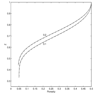
Figure 3: Comparison of asymptotic solutions (54) and (56) (dashed curves) at $t=10$ for $\lambda=1000$ with numerical results (solid curves) in the top region ($Z=z/h(t)\sim 1$ or $z\sim h(t)$) where the profile is nearly at equilibrium state. The curves are calculated for two typical thermal gradients of $\bar{\beta}=0.1,\,0.2$, and the agreement is clearly shown.

where $A=\sqrt{(\dot{m}-\dot{h})(1-\phi_{0})}$. The comparison of viscous solutions (54) and (56) with the numerical results is shown in Figure 3 in the top region where the compaction profile is nearly at equilibrium state for $\lambda=1000$ and $t=10$ for two typical thermal gradients $\bar{\beta}=0.1,\,0.2$. The agreement verifies the numerical method and the asymptotic solution procedure.

4.3 Comparison With Real Data

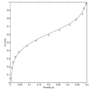
Figure 4: Comparison of numerical simulations (solid curves) with real borehole log data (with $\circ$). $Z=z/h(t)$ is the scaled height. The best fitted values are $\lambda=250$, $m=7.3$, $\bar{\beta}=0.14$, and $t=4.3$.

The numerical simulations and its comparison with real data are shown in Figure 4. The solid curve is the numerical results and real data are depicted by $\circ$. The real data are the borehole log data with a total depth of 3700 m in South China Sea. The rescaled height $Z=z/h(t)$ varies from $0$ to $1$ corresponds to a depth of 3700 m at basement to the ocean floor. In this simulation, we got best fitted values of $\lambda=250$, $m=7.3$, $\bar{\beta}=0.14$, and $t=4.3$ (or real time scale 14.2 Ma).

We can see that porosity near the basin top decrease nearly parabolically with depth, and the porosity reduction only becomes significant at the depth $h-z\sim\Pi$ derived from solution (54) when its right hand $\sqrt{2(1-\phi_{0})/\pi(\dot{m}-\dot{h})}(h-z)=O(1)$, that is

$$\Pi=d\sqrt{\frac{\pi(\dot{m}-\dot{h})}{2(1-\phi_{0})}},$$ (57)

which is about $980$ m for $\phi_{0}=0.4$ and $\dot{m}-\dot{h}=0.37$. In other words, pressure solution becomes only significant at the depths greater than $\Pi$, which is consistent with the real data.

5 Discussions

The present model of pressure solution in sedimentary basins incorporates the effect of temperature gradient in the frame of viscous compaction. Based on the pseudo-steady state approximations in the grain boundary diffusion process, we have been able to formulate a new derivation of viscous compaction relation by using more realistic boundary conditions adjacent grain contacts. The nondimensional model equations are mainly controlled by two parameters $\lambda$, which is the ratio of hydraulic conductivity to the sedimentation rate, and the thermal gradient $\bar{\beta}$. Following the similar asymptotic analysis [5], we have been able to obtain the approximate solutions for either slow compaction ($\lambda\ll 1$) or fast compaction ($\lambda\gg 1$). The more realistic and yet more interesting case is when small (but realistic) temperature gradient $\bar{\beta}\ll 1$ and $\lambda\gg 1$, and the equilibrium solution implies a near parabolic profile of porosity versus depth. Temperature gradient is a very large factor controlling compaction process, but it is only of second importance in the sense that it does not influence the parabolic shape of compaction curves since the shape is mainly characterized by $\lambda$. However, for the same value of $\lambda$ at the same time, the individual curve of the compaction profile is essentially described by the thermal gradient.

The numerical simulations and asymptotic analysis have shown that porosity-depth profile is near parabolic followed by a sudden switch of nearly uniform porosity because $\lambda(\phi/\phi_{0})^{m}$ may become small (even $\lambda\gg 1$ due to the big exponent $m$) at sufficiently large depths. In this case, the porosity profile consists of an upper part near the surface where the equilibrium is attained, and a lower part where the porosity is higher than equilibrium which appears to correspond accurately to numerical computations. In the near equilibrium region, the effect of temperature gradient is very distinguished, the higher the gradient, the quicker the compaction proceeds. On the other hand, once in the nearly uniform lower region, the porosity is essentially uniform, the effect of thermal gradient is not important and negligible, which is consistent with previous numerical simulations [1]. In fact, the permeability becomes so small that fluid gets trapped below this region, and compaction virtually stops.

Acknowledgements. I would like to thank the referees for their very helpful comments and very instructive suggestions. I also would like to than Prof. Andrew C Fowler for his very helpful direction on viscous compaction.

References

1

C. L. Angevine and D. L. Turcotte, Porosity reduction by pressure solution: A theoretical model for quartz arenites, Geol. Soc. Am. Bull., 94, 1129-1134(1983).

2

R. E. Gibson, G. L. England and M. J. L. Hussey, The Theory of One-dimensional Consolidation of Saturated Clays, I. Finite Non-linear Consolidation of Thin Homogeneous Layers, Can. Geotech. J., 17(2)261-273(1967).

3

D. M. Audet and A. C. Fowler, A Mathematical Model for Compaction in Sedimentary Basins, Geophys. Jour. Int., 110 (3) 577-590(1992).

4

A. C. Fowler and X. S. Yang, Fast and Slow Compaction in Sedimentary Basins, SIAM Jour. Appl. Math., 59(1)365-385(1998).

5

A. C. Fowler and X. S. Yang, Pressure Solution and Viscous Compaction in Sedimentary Basins, J. Geophys. Res., B 104, 12 989-12 997 (1999).

6

I. Shimuzu, Kinetics of Pressure Solution Creep in Quartz, Tectonophysics, 245(1)121-134(1995).

7

E. H. Rutter, Pressure Solution in Nature, Theory and Experiment, J. Geol. Soc. London, 140(4)725-740(1976).

8

R. Tada, and R. Siever, Pressure solution during diagenesis, Ann. Rev. Earth Planet. Sci., 17, 89-118 (1989).

9

X. S. Yang, Mathematical Modelling of Compaction and Diagenesis in Sedimentary Basins, D.Phil Thesis, Oxford University (1997).

10

A. M. Mullis, The Role of Silica Precipitation Kinetics in determining the Rate of Quartz Pressure Solution, J. Geophys. Res., 96(7)1007(1991).

11

M.D. Zoback, R. Apel, J. Baumgartner, M. Brudy,R. Emmermann, B. Engeser, K. Fuchs,W. Kessels, H. Rischmuller, F. Rummel and L. Vernik, Upper-crustal strength inferred from stress measurements to 6km depth in the KTB borehole, Nature, 365, 633-635 (1993).

12

T. Dewers and A. Hajash, Rate laws for water-assisted compaction and stress-induced water-rock interaction in sandstones, J. Geophys. Res., B100, 13093-112 (1995).

13

P. Ortoleva, Geochemical self-organization, Oxford University Press, 1994.

14

F. Schneider, J. L. Potdevin, S. Wolf, & I. Faille, Mechanical and chemical compaction model for sedimentary basin simulators, Tectonophysics, 263, 307-317 (1996).

15

R. H. Lander, O. Walderhaug, Predicting porosity through simulating sandstone compaction and quartz cementation, Bull. Amer. Assoc. Petrol. Geol., 83, 433-449(1999).

16

A Revil, Pervasive pressure-solution transfer: a poro-visco-plastic model, Geophys. Res. Lett., 26, 255-258 (1999).

17

H. Pape, C. Clauser and J. Iffland, Permeability prediction based on fractal pore-space geometry, Geophysics, 64, 1447-1460 (1999).

18

J. E. Smith, The dynamics of shale compaction and evolution in pore-fluid pressures, Math. Geol., 3, 239-263(1971).

Figure 2: The basin thickness $h(t)$ as a function of time $t$ for different values of $\lambda=0.1,10,1000$. It clearly show that the moving boundary $z=h(t)$ increases almost linearly with time $t$, which implies that $\dot{h}=const$ depending only on $\lambda$.