Higher-order Statistics of Weak Lensing Shear and Flexion

Abstract

Owing to their more extensive sky coverage and tighter control on systematic errors, future deep weak lensing surveys should provide a better statistical picture of the dark matter clustering beyond the level of the power spectrum. In this context, the study of non-Gaussianity induced by gravity can help tighten constraints on the background cosmology by breaking parameter degeneracies, as well as throwing light on the nature of dark matter, dark energy or alternative gravity theories. Analysis of the shear or flexion properties of such maps is more complicated than the simpler case of the convergence due to the spinorial nature of the fields involved. Here we develop analytical tools for the study of higher-order statistics such as the bispectrum (or trispectrum) directly using such maps at different source redshift. The statistics we introduce can be constructed from cumulants of the shear or flexions, involving the cross-correlation of squared and cubic maps at different redshifts. Typically, the low signal-to-noise ratio prevents recovery of the bispectrum or trispectrum mode by mode. We define power spectra associated with each multispectra which compresses some of the available information of higher order multispectra. We show how these can be recovered from a noisy observational data even in the presence of arbitrary mask, which introduces mixing between Electric (${\rm E}$-type) and Magnetic (${\rm B}$-type) polarization, in an unbiased way. We also introduce higher order cross-correlators which can cross-correlate lensing shear with different tracers of large scale structures.

1 Introduction

Weak lensing surveys play an important role as cosmological probes complementary to Cosmic Microwave Background (CMB) surveys and large-scale galaxy surveys. In principle, they can probe evolution of the dark matter power spectrum at a moderate redshifts in an unbiased way; for a recent review, see Munshi et al. (2008). However, the first weak lensing measurements were published within the last decade (Bacon, Refregier & Ellis, 2000; Wittman et al, 2000; Kaiser, Wilson & Luppino, 2000; Waerbeke et al, 2000) so this is a young field. There has been a tremendous progress in the last decade since the first measurements, on various fronts, including analytical modeling, technical specification and the control of systematics. Weak lensing probes cosmological perturbations on smaller angular scales where the perturbations are both nonlinear and non-Gaussian. The two-point correlation function (or, equivalently, the power spectrum) of weak lensing is weakly sensitive to the cosmological constant $\Omega_{\Lambda}$. It also depends only on a degenerate combination of amplitude of matter power spectrum $\sigma_{8}$ and the matter density parameter $\Omega_{M}$. This degeneracy can be broken by use of the three-point correlation function which is diagnostic of the non-Gaussianity induced by gravity (Villumsen, 1996; Jain & Seljak, 1997).

The higher order statistics needed to analyze weak lensing in detail are however prone to the effects of noise due to the intrinsic ellipticity distribution, finite number of galaxies (shot noise) and sample (or cosmic) variance owing to the partial sky coverage. Ongoing and planned weak lensing surveys, such as the CFHT legacy survey, Pan-STARRS , the Dark Energy Survey, and further in the future, the Large Synoptic Survey Telescope , JDEM and Euclid will provide a wealth of information in terms of mapping the distribution of mass and energy in the universe. A large fractional sky coverage as well as accurate photometric redshift determination will help to probe higher order correlation functions at a higher signal-to-noise(S/N) then is possible at present (see e.g. Pen et al. (2003)).

Almost all previous studies concerning weak lensing have used a real space description and employed correlation function of various orders to probe underlying mass clustering. Future surveys will cover a good fraction of the sky, if not the entire sky. This motivates us to use a harmonic description and employ the mutispectra - which are simply the Fourier representations of the higher order correlation functions. Weak lensing observations require masks with complicated topology to deal with presence of foreground objects. Our formalism in harmonic space can deal with arbitrary mask. The formalism described here is completely general and can deal with fields with arbitrary spins including shear and flexions.

In the absence of information concerning the redshifts of the source galaxies, traditional weak lensing studies have tended to operate in projection or in 2D slices. Indeed, before the advent of 3D weak lensing, almost all studies were carried out in such a way (Jain, Seljak & White, 2000). Due to lack of all-sky coverage most studies also used a “flat sky” approach (Munshi & Jain (2001); Munshi (2000); Munshi & Jain (2000)) which has led to study of lower order non-Gaussianity using convergence $\kappa$ as well as shear $\gamma$ Munshi & Jain (2001); Valageas (2000); Munshi & Valageas (2005); Valageas, Barber, & Munshi (2004); Valageas, Munshi, & Barber (2005). As the next stage of development tomographic approaches went beyond projected survey by binning galaxies in redshift slices which can further tighten the constraints Takada & White (2003); Takada & Jain (2004). More recently, the use of photometric redshifts to study weak lensing in three dimensions was introduced by Heavens (2003). It was later developed by many authors Heavens et al. (2000); Heavens et al (2006); Heavens, Kitching & Verde (2007); Castro et al (2005), and was shown to be a vital tool in constraining dark energy equation of state (Heavens et al, 2006), neutrino mass (Kitching et al., 2008) and many other possibilities. In our present study we propose estimators for non-Gaussianity using projected data.

In most cosmological studies, the power spectrum remains the most commonly used statistical probe and its evolution and characterization remain the best studied. As has already been pointed out, however, higher order statistics can help to break degeneracies e.g. in $\Omega_{M}$ and $\sigma_{8}$, but are more difficult to probe observationally (see e.g. Bernardeau, van Waerbeke & Mellier (1997); Jain & Seljak (1997); Hui (1999); Schneider et al (2002); Takada & Jain (2003)) given the low signal to noise associated with them. As a result most commonly used higher order probes compress the available information to a simple number (e.g. “skewness” or “kurtosis”) which are one-point statistics (Pen et al., 2003). The higher order correlation functions have been detected observationally (Bernardeau, van Waerbeke & Mellier, 1997; Bernardeau, Mellier & Van Waerbeke, 2002) and future larger samples are expected to improve the statistical situation still further. A recent study by Munshi, Heavens & Coles (2010) has underlined the usefulness of working with two-point correlations (or their Fourier analog the power spectrum) at each order. At the level of the bispectrum, a single power spectrum tends to compress some of the available information; there is more than one degenerate power spectrum associated with the higher order multispectra. We extend the recent study by Munshi, Heavens & Coles (2010) and provide systematic results at each order for spin$-2$ fields, thus generalizing our previous results for spin-$0$ fields such as the convergence. Understanding higher order statistics also provide an indication of the scatter associated with estimation of lower order statistics Takada & Jain (2009). Their results extend the formalism developed in Heavens (2003) and Castro et al (2005) and we follow the all-sky expansion introduced in weak lensing studies by Stebbins (1996).

Statistics of the shear $\gamma$ or convergence $\kappa$ seen in a lensing map are sensitive to the statistics of underlying density contrast $\delta={\delta\rho_{b}/\rho_{b}}$ of background density $\rho_{b}$. An accurate understanding of the gravitational clustering is therefore essential for modeling the weak lensing statistics. At present we lack a detailed analytical model of the non-linear gravitational clustering. In the absence of a clear analytical picture, beyond the perturbative regime the modeling of the higher order statistics are done using a hierarchical ansatz (see e.g. Fry (1984); Schaeffer (1984); Bernardeau & Schaeffer (1992); Szapudi & Szalay (1993, 1997); Munshi et al (1999); Munshi, Coles & Melott (1999a, b); Munshi, Melott & Coles (1999); Munshi & Coles (2000, 2002, 2003)). The hierarchical ansatz assumes a factorisable model for the higher order correlation functions. Different hierarchical ansatze differs the way they assign amplitudes to the various tree amplitudes. We will employ a very generic form of the hierarchical ansatz which has already been tested in modeling of projected statistics. The method is flexible enough to allow for a more specific prescription. Other approaches to model nonlinear gravity include the halo models (Cooray & Seth, 2002) which has also been employed in weak lensing studies.

In a recent paper, Munshi, Heavens & Coles (2010) advocated the use of higher order cumulants and their correlators of convergence $\kappa$ along with their associated power spectra for studying dark matter clustering beyond power spectra in 3D. The aim of the present paper is to extend that study to fields with non-zero spin (e.g. shear). Shear can directly be used from observed data to study the dark matter clustering beyond the usual approximation of Gaussianity. Although in this study we primarily focus on shear, the analytical results are directly applicable for higher order spin fields sometime used in weak lensing known as flexions. Previous studies have also focused on the cumulant correlators of the shear $\gamma$ and $\kappa$ (Bernardeau, van Waerbeke & Mellier, 1997; Bernardeau, Mellier & Van Waerbeke, 2002; Bernardeau, Mellier & van Waerbeke, 2003). While cumulant correlators for convergence fields can be probed in a relatively straight forward manner, even to arbitrary order (Munshi, 2000), the analogous studies are more involved for shear fields. There have been some studies involving smoothed $M_{ap}$ statistics to study cumulant correlators from shear map by using compensated filters (Munshi & Valageas, 2005), but in this present paper we develop a more systematic approach to probe higher order statistics directly through spinorial objects. The focus of the present study is to develop tools in the Fourier domain and to use the power spectra associated with the multispectra as opposed to cumulant correlators. Given the non-trivial topology of weak lensing surveys correlation functions indeed are a good option to work with, but, as we will show, the power spectra we develop can also be estimated in the presence of arbitrary mask and noisy data.

The paper is arranged as follows. In §2 we discuss the basic formalism and introduce some terminology and notation. In §3, we introduce the power spectra related to bispectra and trispectra for various combinations of the convergence, shear as well as flexion fields. In §4 we focus on statistical description of underlying matter distribution and relate them to power spectra defined in previous sections for weak lensing observables. Finally §5 is reserved for discussions and future prospects.

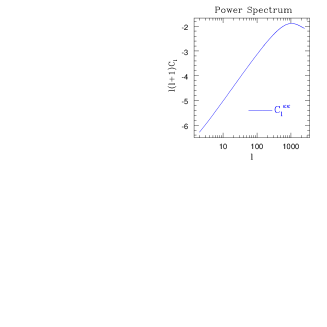
Figure 1: The plots correspond to the power spectrum of convergence $C_{l}^{\kappa\kappa}$. The source redshift is $z_{1}=z_{2}=1$. See text for more details.

2 Convergence, Shear and Flexions

Among the observables including in weak lensing studies are the convergence $\kappa({\hat{\Omega}})$, shear $\gamma({\hat{\Omega}})$ and flexions ${\cal F}({\hat{\Omega}}),{\cal G}({\hat{\Omega}})$. The harmonic decomposition needed in all-sky calculations involves spin-weight spherical harmonics for such objects. We introduce the basic notations in this section following Castro et al (2005). We will ignore the radial dependence for this work as we mainly concentrate on projected surveys. The results presented here will extend the results in (Munshi, Heavens & Coles, 2010) wherein only scalar fields were considered. Though the analysis here follows full spherical decomposition it is indeed possible to choose a rectangular coordinate system which can simplify the calculation for surveys observing a small patch of the sky.

2.1 Spin-weight Spherical Harmonics

We start by introducing the spin-weight spherical harmonics ${}_{s}Y_{lm}({\hat{\Omega}})$ that can be expressed in terms of the Wigner-D function (see e.g. Varshalovich, Moskalev & Khersonskii (1988); Penrose & Rindler (1984,1986) for a detailed discussion). They form a complete and orthonormal set of function on the surface of the celestial sphere. Any spin-weighted function ${}_{s}f({\hat{\Omega}})$ can be decomposed into harmonics ${}_{s}f_{lm}$ using spin-weight spherical harmonics:

$${}_{s}Y_{lm}({\hat{\Omega}})=\sqrt{\frac{2l+1}{4\pi}}D^{l}_{-s,m}(\theta,\phi,0);\qquad{}_{s}f({\hat{\Omega}})=\sum_{lm}{}_{s}Y_{lm}({\hat{\Omega}}){}_{s}f_{lm}.\\$$ (1)

The spin-weighted spherical harmonics ${}_{s}Y_{lm}({\hat{\Omega}})$ (defined only for $|s|>l$ )can be seen as a generalization of the scalar, vector and tensor, spherical harmonics (Varshalovich, Moskalev & Khersonskii, 1988) satisfying the following orthogonality and completeness relations:

$$\sum_{lm}{}_{s}Y_{lm}({\hat{\Omega}}){}_{s^{\prime}}Y_{lm}({\hat{\Omega}}^{\prime})=\delta_{D}({\hat{\Omega}}-{\hat{\Omega}}^{\prime});\qquad\int d{\hat{\Omega}}~{}{}_{s}Y_{lm}({\hat{\Omega}}){}_{s^{\prime}}Y_{l^{\prime}m^{\prime}}({\hat{\Omega}})=\delta^{K}_{ss^{\prime}}\delta^{K}_{ll^{\prime}}\delta^{K}_{mm^{\prime}}.$$ (2)

Here $\delta^{K}$ is the Kronecker delta function and $\delta_{D}$ is a Dirac delta function. The spin raising operator “edth”, $\,\eth\,$ and its complex conjugate, the spin lowering operator $\bar{\,}\eth\,$ are defined through their action on spin spherical harmonics which can be used to define spin-weighted harmonics ${}_{s}Y_{lm}({\hat{\Omega}})$ from ordinary spherical harmonics $Y_{lm}({\hat{\Omega}})$. The spin spherical harmonics ${}_{s}Y_{lm}({\hat{\Omega}})$ are the eigen functions of the operator $\,\eth\,\bar{\,}\eth\,$. Note that $\,\eth\,$ can be thought also as an effective covariant derivative on the surface of the sphere which generates quantities related to the various spins:

$$\,\eth\,{}_{s}Y_{lm}=[(l-s)(l+s+1)]^{1/2}{}_{s+1}Y_{lm};\qquad\bar{\,}\eth\,{}_{s}Y_{lm}=[(l+s)(l-s+1)]^{1/2}{}_{s-1}Y_{lm}.$$ (3)

This also implies that $\,\eth\,\bar{\,}\eth\,{}_{s}Y_{lm}=[(l-s)(l+s+1)]{}_{s}Y_{lm}$ and $\,\eth\,\bar{\,}\eth\,{}_{s}Y_{lm}=[(l+s)(l-s+1)]{}_{s}Y_{lm}$. The conversion between convergence and shear harmonics used the following expression which we will also be using later:

$$\,\eth\,\,\eth\,Y_{lm}({\hat{\Omega}})=\sqrt{(l+2)!\over(l-2)!}{}_{2}Y_{lm}({\hat{\Omega}});\qquad\qquad\bar{\,}\eth\,\bar{\,}\eth\,Y_{lm}({\hat{\Omega}})=\sqrt{(l+2)!\over(l-2)!}{}_{-2}Y_{lm}({\hat{\Omega}}).$$ (4)

The operators $\,\eth\,$ and $\bar{\,}\eth\,$ are convenient for expressing the spin weight objects which are coordinate frame dependent in terms of ones which are frame independent or scalars. All invariant differential operators on the sphere may be expressed in terms of $\,\eth\,$ and $\bar{\,}\eth\,$.

The following overlap integrals will be useful in our future derivations which will be used to derive the expressions for bispectrum and trispectrum related power spectrum.

$$\int{}_{s}Y_{lm}({\hat{\Omega}}){}_{s^{\prime}}Y_{l^{\prime}m^{\prime}}({\hat{\Omega}}){}_{s^{\prime\prime}}Y_{l^{\prime\prime}m^{\prime\prime}}({\hat{\Omega}})d{\hat{\Omega}}=S_{ll^{\prime}l^{\prime\prime}}\left(\begin{array}[]{ c c c }l&l^{\prime}&l^{\prime\prime}\\ m&m^{\prime}&m^{\prime\prime}\end{array}\right)\left(\begin{array}[]{ c c c }l&l^{\prime}&l^{\prime\prime}\\ -s&-s^{\prime}&-s^{\prime\prime}\end{array}\right);\qquad S_{ll^{\prime}l^{\prime\prime}}\equiv\sqrt{(2l+1)(2l^{\prime}+1)(2l^{\prime\prime}+1)\over 4\pi}.$$ (5)

The above result can be cast in following form which is useful for expressing integrals of more than three spin spherical harmonics in terms of Wigner $3j$ symbols when dealing with trispectrum or multispectra of even higher order.

$${}_{s}Y_{lm}({\hat{\Omega}}){}_{s^{\prime}}Y_{lm}({\hat{\Omega}})=\sum_{LSM}{}_{S}Y^{*}_{LM}S_{Ll^{\prime}l^{\prime\prime}}\left(\begin{array}[]{ c c c }L&l^{\prime}&l^{\prime\prime}\\ M&m^{\prime}&m^{\prime\prime}\end{array}\right)\left(\begin{array}[]{ c c c }L&l^{\prime}&l^{\prime\prime}\\ -S&-s^{\prime}&-s^{\prime\prime}\end{array}\right).$$ (6)

These results are generalizations of similar results often used in the context of scalar (spin-$0$) harmonics which can be recovered by setting $s=s^{\prime}=s^{\prime\prime}=0$. In a small patch of sky, a rectangular coordinate system can be introduced which can simplify some of the calculations and might be useful for surveys with small sky coverage. A detailed analysis will be presented elsewhere (Munshi et al. (2010) in preparation).

2.2 Harmonic decomposition of Convergence and Shear

We start by defining the complex shear $\gamma$ in terms of the individual shear components $\gamma_{1}$ and $\gamma_{2}$ at a given angular position $\Omega=(\theta,\phi)$ and at a radial line-of-sight distance $|{\bf r}|=r$ (see Munshi et al. (2008) for a more detailed discussion and definitions). We will closely follow the notations of (Castro et al, 2005) where possible. We will not Fourier decompose in the radial direction. The harmonic decomposition is performed only the surface of the celestial sphere

$$\gamma_{\pm}({\hat{\Omega}},r)=\gamma_{1}({\hat{\Omega}},r)\pm i\gamma_{2}({\hat{\Omega}},r).$$ (7)

It is customary to define a complex lensing potential $\phi(r)=\phi_{E}(r)+i\phi_{B}(r)$ which is related to the line-of-sight integration of the peculiar gravitational potential $\phi$ and to define the shear in terms of spin-derivatives $\eth$ and its conjugate $\bar{\eth}$ of $\phi$. The action of $\eth$ is to raise the spin whereas $\bar{\eth}$ reduces the spin of the object it is acting on. This operator was first introduced by Varshalovich, Moskalev & Khersonskii (1988); Penrose & Rindler (1984,1986) on the surface of the sphere in order to define the now widely used spin-weight $s$ spherical harmonics which live on the surface of a sphere

$$\gamma({\bf r})={1\over 2}\eth\eth[\phi_{E}({\bf r})+i\phi_{B}({\bf r})];\qquad\gamma^{*}({\bf r})={1\over 2}{\bar{\eth}}{\bar{\eth}}[\phi_{E}({\bf r})-i\phi_{B}({\bf r})].\qquad$$ (8)

Explicit expressions for these spin-lowering and raising differential operators are given in Castro et al (2005). While acting on a complex scalar potential $\phi$, the fields $\gamma({\bf r})$ generates the $\gamma({\bf r})$ and its conjugate which are of spin $+2$ and $-2$ respectively. In later sections we will use the generalized symbol ${}_{s}\Gamma$ for general spin fields which will include products of shear fields as well as higher derivative spin fields such as flexions. In our current notation ${}_{2}\Gamma=\gamma$ and ${}_{-2}\Gamma=\gamma^{*}$:

$${}_{2}\Gamma({\bf r})\equiv\gamma({\bf r})={1\over 2}\eth\eth\phi({\bf r});\qquad{}_{-2}\Gamma({\bf r})\equiv\gamma^{*}({\bf r})={1\over 2}\bar{\eth}\bar{\eth}\phi^{*}({\bf r}).$$ (9)

The individual shear components $\gamma_{1}({\bf r})$ and $\gamma_{2}({\bf r})$ can be expressed in terms of a complex lensing potential $\phi({\bf r})=\phi_{E}({\bf r})+i\phi_{B}({\bf r})$. The magnetic part of the potential $\phi_{B}({\bf r})$ will take contribution mainly from systematics and electric part corresponds to pure lensing contribution

$$\gamma_{1}({\bf r})={1\over 4}(\,\eth\,\,\eth\,+\bar{\,}\eth\,\bar{\,}\eth\,)\phi({\bf r});\qquad\gamma_{2}({\bf r})=-{i\over 4}(\,\eth\,\,\eth\,-\bar{\,}\eth\,\bar{\,}\eth\,)\phi({\bf r});\qquad\kappa({\bf r})={1\over 4}(\,\eth\,\bar{\,}\eth\,+\,\eth\,\bar{\,}\eth\,)\phi({\bf r}).$$ (10)

The harmonics of $\gamma$ and $\gamma^{*}$ can be expressed in terms of the harmonics coefficients of $\Phi_{E}$ and $\Phi_{B}$ denoted by $E_{lm}$ and $B_{lm}$ respectively.

$${}_{2}\Gamma_{lm}=-[E_{lm}+iB_{lm}];\qquad{}_{-2}\Gamma_{lm}=-[E_{lm}-iB_{lm}].$$ (11)

The spinorial fileds can likewise be expanded in an appropriate basis which uses the spin-spherical harmonics ${}_{s}Y_{lm}({\hat{\Omega}})$. For the case of ${}_{2}\Gamma_{lm}$ we have the following expression:

$${}_{\pm 2}\Gamma({\bf r})=\sum_{l=0}^{\infty}\sum_{m=-l}^{l}\sqrt{(l+2)!\over(l-2)!}~{}\phi_{lm}~{}{}_{\pm 2}Y_{lm}(r,{\hat{\Omega}}).$$ (12)

We will be only dealing with 2D part of the spherical expansion as we will be dealing with projected surveys in this work. The harmonics $E_{lm}$ and $B_{lm}$ are harmonic components of Electric (E) and Magnetic (B) fields respectively. In the absence of B-mode the harmonics of the shear components are directly related to the harmonic component of the Electric field $E_{lm}$. The harmonic transforms of the shear components and convergence are linked to the lensing potential $\phi$ as follows:

$$E_{lm}(k)=-{1\over 2}\sqrt{(l+2)!\over(l-2)!}\phi_{lm}(k)\qquad\kappa_{lm}(k)=-{l(l+1)\over 2}\phi_{lm}(k).$$ (13)

These expression are useful in relating the bi- or trispectrum of various quantities in terms of the convergence ones.

2.3 Harmonic Decomposition of Flexions

Higher spin objects known as flexions are sometimes also used to study weak lensing; they are related to derivatives of the shear (Goldberg & Natarajan (2002); Goldberg & Beacon (2005); Bacon et al. (2006); Bacon & Goldberg (2005); Schneider & Er (2008)). There are two flexions which are typically used; $\cal F$ also known as the first flexion (spin -$1$) and $\cal G$ which is also known as the second flexion (spin -$3$). The combinations of these two flexions can specify the weak “arciness” of the lensed image and hence can quantify the lensing distortion beyond that encoded in shear. Their relationship with the shapelet formalism have been discussed at length (Refregier, 2003; Bernstein & Jarvis, 2002; Refregier & Beacon, 2003). Both flexions have been used extensively in the literature for individual halo profiles and also for the study of substructures (Bacon et al., 2006). Our aim here, as it is in the case of shear, is to focus mainly on higher order statistics of these objects for generic underlying cosmological clustering. We will do so by expressing the bispectrum of the shapelets in terms of that of the convergence $\kappa$, as we did for shear $\gamma$. The first and the second flexions $\cal F$ and $\cal G$ can be derived from the lensing potential $\phi({\bf r})$ (Castro et al, 2005) by the use of the lowering and raising operators:

$${\cal F}({\bf r})={1\over 6}\left(\bar{\,}\eth\,\,\eth\,\,\eth\,+\,\eth\,\bar{\,}\eth\,\,\eth\,+\,\eth\,\,\eth\,\bar{\,}\eth\,\right)\phi({\bf r});\qquad{\cal G}({\bf r})={1\over 2}\bar{\,}\eth\,\bar{\,}\eth\,\bar{\,}\eth\,\phi({\bf r}).$$ (14)

Flexions have been used primarily to measure the galaxy-galaxy lensing to probe the galaxy halo density profiles. Their cosmological use will depend on an accurate understanding of gravitational clustering at small angular scales. In Fourier space we will denote the harmonics of $\cal F$ and $\cal G$ by ${\cal F}_{lm}$ and ${\cal G}_{lm}$ and we can use the Eq.(4) to express them in terms of the $\phi_{lm}$.

$${\cal F}_{lm}={1\over 6}l^{1/2}(l+1)^{1/2}\left(3l^{2}+3l-2\right)\phi_{lm};\qquad{\cal G}_{lm}={1\over 2}\sqrt{(l+3)!\over(l-3)!}\phi_{lm}$$ (15)

Though we will primarily be focusing on higher order statistics of shear the results are equally applicable for flexions (which generalize the concept of shear). In addition to the shear statistics we will also consider a scalar field in our analysis $\Psi$. We will leave this, which can represent a suitable large scale tracer, arbitrary. The resulting analysis depends on the multispectra involving both the weak lensing shear field and that of the tracer fields. The flexions put more weight on smaller scales, where the hierarchical ansatz is known to be more accurate, so the formalism we develop here will also be suitable for them. It is also possible to use our general results to construct estimators for mixed bispectra involving shear and flexions.

However we should also point out that the modeling of intrinsic flexions of source galaxies, which is the main contribution to the noise, is difficult. This will depend heavily on modeling of galaxy shapes beyond the simplest description of their intrinsic shear. This uncertainty is expected to increase with survey depth. A detailed modeling and optimization of survey strategy will be presented elsewhere.

3 Higher Order Statistics of Weak Lensing Shear and Flexion

The Higher order statistics encodes the departure from Gaussianity. The non-Gaussianity probed by any cosmological observations can either be a primary one due to initial conditions or a secondary one which in case of weak lensing is mainly induced by subsequent gravitational instability responsible for structure formation. At lower redshift it is expected that the secondary non-Gaussianity will dominate the primary one. The estimation of non-Gaussianity using higher order correlation functions are typically dominated by noise. The higher order correlation functions or their Fourier transforms (multispectra) contains a wealth of information. Some of these information however can be degenerate due to large number of possible configurations in real or Fourier domain. Typically one-point statistics e.g. skewness or kurtosis that are used compress all possible information to a single number thereby increasing the Signal-to-Noise but reducing the information content. As a next step, collapsed two-point objects (or cumulant correlators) which are higher order objects are also used (Munshi, 2000). They are easier to recover from a noisy data than the complete correlation functions. The Fourier transforms of these two-point cumulant correlators are the power spectrum associated with a specific choice of the multispectra. There can be more than one power spectra for any specific choice of multispectra. In this section we derive power spectra associated with bispectra and trispectra for shear as well as flexions.

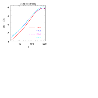
Figure 2: The plots correspond to the bispectrum related power spectrum $C_{l}^{(2,1)}$. Various curves correspond to the spectra $C_{l}^{\kappa\kappa,\kappa}$, $C_{l}^{\kappa\kappa,\gamma_{+}}$, $C_{l}^{\kappa\gamma_{+},\gamma_{+}}$ and $C_{l}^{\gamma_{+}\gamma_{+},\gamma_{+}}$ as depicted. The source redshift is $z_{1}=z_{2}=1$. See text for details.

3.1 Power spectrum associated with the Bispectrum

The bispectrum is the lowest in the hierarchy of multispectra and have the highest Signal-to-Noise. There has been lot of interest in modeling and detection of weak lensing bispectrum mainly using convergence maps as well as shear. As remarked earlier, shear correlation functions are more complicated and have rich patterns given their spinorial nature. They have been studied in real space for specific triplet configurations analytically (Bernardeau, Mellier & Van Waerbeke, 2002) and have been measured in real surveys (Bernardeau, Mellier & van Waerbeke, 2003) for first detection of non-Gaussianity signal from weak lensing observations. Bernardeau (2005) has also provided analytical results for more general configurations but in an idealistic one-halo configuration. In this paper we focus on the power spectra associated with bispectra to probe higher order correlation hierarchy in studying gravity induced non-Gaussianity. Our results are completely general and given any models of underlying bispectrum can predict observed power spectrum related to bispectrum in the presence of arbitrary observational mask. We will assume noise to be Gaussin through out and will not contribute to the bispectrum.

3.1.1 The Two-to-One Power spectrum: $C_{l}^{(2,1)}$

We will start by considering two fields on a surface of a sphere ${{}_{s}\Gamma}({\hat{\Omega}})$ and ${{}_{s^{\prime}}\Gamma^{\prime}}({\hat{\Omega}})$, which are respectively of spin $s$ and $s^{\prime}$. These objects can be the shear, $\gamma_{\pm}$, flexions, $\cal F$, $\cal G$ or a tracer field $\Psi$. The resulting product fields such as e.g. $\gamma_{+}\gamma_{-}$ can be of spin zero, on the other hand $\gamma_{+}^{2}$ and $\gamma_{-}^{2}$ are of spin $-4$ and $+4$ respectively. The results can also involve fields such as $\Psi\gamma_{+}$ which is a spin $-2$ field. A spin $s$ field can be decomposed using spin-harmonics ${}_{s}Y_{lm}({\hat{\Omega}})$. These spin harmonics are generalization of ordinary spherical harmonics $Y_{lm}({\hat{\Omega}})$ which are used to decompose the spin-$0$ (or scalar) functions e.g. $\Psi({\hat{\Omega}})$ defined over a surface of a sphere (sky). Throughout we will be using lower case symbols $s,s^{\prime}$ to denote the spins associated with the corresponding fields denoted in italics. The fields that are constructed from various powers of $\gamma_{+}$ and $\gamma_{-}$ can be expanded in terms of the corresponding spin-harmonics basis ${}_{s}Y_{lm}({\hat{\Omega}})$. The product field such as $[{{}_{s}\Gamma}({\bf r}){{}_{s^{\prime}}\Gamma^{\prime}}({\bf r})]$ which is of spin $s+s^{\prime}$ can therefore be expanded in terms of the harmonics ${}_{s+s^{\prime}}Y_{lm}({\hat{\Omega}})$. The following relationship therefore expresses the harmonics of the product field in terms of the harmonics of individual fields .

$$[{{}_{s}\Gamma}({\bf r}){{}_{s^{\prime}}\Gamma^{\prime}}({\bf r})]_{lm}=\int d{\hat{\Omega}}{{}_{s}\Gamma}({\bf r}){{}_{s^{\prime}}\Gamma^{\prime}}({\bf r})[{}_{s+s^{\prime}}Y_{lm}^{*}({\hat{\Omega}})]=\sum_{l_{i}m_{i}}{}_{s}\Gamma_{l_{1}m_{1}}(r){}_{s^{\prime}}\Gamma^{\prime}_{l_{2}m_{2}}(r)\int[{}_{s}Y_{l_{1}m_{1}}({\hat{\Omega}})][{}_{s^{\prime}}Y_{l_{2}m_{2}}({\hat{\Omega}})][{}_{s+s^{\prime}}Y_{lm}^{*}({\hat{\Omega}})]d{\hat{\Omega}};{}$$

$$=\sum_{l_{i}m_{i}}{}_{s}\Gamma_{l_{1}m_{1}}(r){}_{s^{\prime}}\Gamma^{\prime}_{l_{2}m_{2}}(r)I_{l_{1}l_{2}l}\left(\begin{array}[]{ c c c }l_{1}&l_{2}&l\\ s&s^{\prime}&-(s+s^{\prime})\end{array}\right)\left(\begin{array}[]{ c c c }l_{1}&l_{2}&l\\ m_{1}&m_{2}&m\end{array}\right);\quad I_{l_{1}l_{2}l}=\sqrt{(2l_{1}+1)(2l_{2}+1)(2l+1)\over 4\pi}$$ (20)

The expression derived above is valid for all-sky coverage. Mixing of Electric-$E$ and Magnetic-$B$ modes results from partial sky coverage. The results will be generalized later to take into account arbitrary partial sky coverage and we will derive exact form for the mixing matrix. We have assumed a Gaussian noise resulting from intrinsic ellipticity distribution of galaxies, however this will not contribute to this non-Gaussianity statistic. We define the associated power spectra to write:

$$C_{l}^{\Gamma\Gamma^{\prime},\Gamma^{\prime\prime}}(r_{1},r_{2})={1\over 2l+1}\sum_{m}[{}_{s}\Gamma{}_{s^{\prime}}\Gamma^{\prime}]_{lm}(r){}_{s^{\prime\prime}}\Gamma^{\prime\prime*}_{lm}(r)$$ (21)

$$\qquad\qquad=\sum_{l_{1}l_{2}}J_{l_{1}l_{2}l}~{}B^{\Gamma\Gamma^{\prime}\Gamma^{\prime}}_{l_{1}l_{2}l}(r_{1},r_{1},r_{2})\left(\begin{array}[]{ c c c }l_{1}&l_{2}&l\\ s&s^{\prime}&-(s+s^{\prime})\end{array}\right);\qquad J_{l_{1}l_{2}l}=\sqrt{(2l_{1}+1)(2l_{2}+1)\over(2l+1)}.$$ (24)

The power spectrum $C_{l}^{\Gamma\Gamma^{\prime},\Gamma^{\prime\prime}}(r_{1},r_{2})$ essentially cross-correlates the product maps at a given radial distance $r_{1}$ to another map at another redshift $r_{2}$ to probe the third order statistics bispectrum $B$. Similar statistics in the coordinate space has been reported before. (Bernardeau, van Waerbeke & Mellier, 2003) studied $\langle\gamma^{2}({\hat{\Omega}})\gamma({\hat{\Omega}}^{\prime})\rangle$ which directly deals with shear maps as opposed to convergence maps. This statistics along with a similar but simpler version which uses $\langle\kappa^{2}({\hat{\Omega}})\kappa({\hat{\Omega}}^{\prime})\rangle$ was studied. They employed perturbation theory to model underlying mass distribution and used a flat sky approximation to simplify their calculations. A complementary statistics $\langle(\gamma({\hat{\Omega}}_{1})\cdot\gamma({\hat{\Omega}}_{2}))\gamma\rangle$ was also considered which relies on more detailed modeling of the bispectrum. These statistics were used by (Bernardeau, Mellier & Van Waerbeke, 2002) later to detect non-Gaussianity from VIRMOS-DESCART Lensing Survey.

Our results presented here deal with power spectrum associated with the higher order multispectra and are derived using generic all-sky treatment and can handle decomposition into Electric and Magnetic components in a much more straightforward manner. Our results are complementary to their analysis. We will also generalize these results to higher order and show how to take into account the mask in a generic way. The results presented here are not only applicable to shear or convergence but are also applicable for higher order spinorials such as Flexions.

We have introduced the bispectrum $B^{\Gamma\Gamma^{\prime}\Gamma^{\prime\prime}}_{l_{1}l_{2}l}(r_{1},r_{2},r_{3})$ in Eq.(24) which can now be related to the harmonics of the relevant fields by the following equation:

$$B_{l_{1}l_{2}l_{3}}^{\Gamma\Gamma^{\prime}\Gamma^{\prime\prime}}(r_{1},r_{2},r_{3})=\sum_{m_{1}m_{2}m_{3}}\langle{}_{s}\Gamma_{l_{1}m_{1}}(r_{1}){}_{s^{\prime}}\Gamma^{\prime}_{l_{2}m_{2}}(r_{2}){}_{s^{\prime\prime}}\Gamma^{\prime\prime}_{l_{3}m_{3}}(r_{3})\rangle_{c}\left(\begin{array}[]{ c c c }l_{1}&l_{2}&l_{3}\\ m_{1}&m_{2}&m_{3}\end{array}\right).$$ (25)

The matrices denote Wigner 3j symbols (Edmonds, 1968) which are only non zero when the quantum numbers $l_{i}$ and $m_{i}$ satisfy certain conditions. For $x=y=0$ this generalizes the results obtained in (Cooray, 2005) valid for the case of scalars (see also Chen & Szapudi (2007) for related discussions). The result derived above is valid for a general $E$ and $B$ type polarization field. Contribution from ($B$-type) magnetic polarization is believed to be considerably smaller compared to the ($E$-type) electric polarization. The results derived above will simplify considerably if we ignore the $B$ type polarization field in our analysis. In general the power spectra described above will not be real though real and imaginary parts can be separated by considering different components of the bispectrum. However if we assume that the magnetic part of the polarization is zero the following equalities will hold:

$$B_{l_{1}l_{2}l_{3}}^{\gamma_{\pm}\Psi\Psi}=F_{l_{1}}B_{l_{1}l_{2}l_{3}}^{\kappa\Psi\Psi};~{}~{}~{}~{}\\ B_{l_{1}l_{2}l_{3}}^{\gamma_{\pm}\gamma_{\pm}\Psi}=F_{l_{1}}F_{l_{2}}B_{l_{1}l_{2}l_{3}}^{\kappa\kappa\Psi};~{}~{}~{}\\ B_{l_{1}l_{2}l_{3}}^{\gamma_{\pm}\gamma_{\pm}\gamma_{\pm}}=F_{l_{1}}F_{l_{2}}F_{l_{3}}B_{l_{1}l_{2}l_{3}}^{\kappa\kappa\kappa}.~{}~{}~{}\\$$ (26)

The result presented above is valid for all-sky coverage. Clearly from practical considerations we need to add a foreground mask. If we consider the masked harmonics associated with the mask, for a given $w({\hat{\Omega}})$ arbitrary mask , then expanding the product field, in the presence of mask, we can write:

$$[{{}_{s}\Gamma}({\bf r}){{}_{s^{\prime}}\Gamma^{\prime}}({\bf r})w({\hat{\Omega}})]_{lm}=\sum_{l_{i}m_{i};l_{a}m_{a}}{}_{s}\Gamma_{l_{1}m_{1}}(r){}_{s^{\prime}}\Gamma^{\prime}_{l_{2}m_{2}}(r)w_{l_{a}m_{a}}\int[{}_{s}Y_{l_{1}m_{1}}({\hat{\Omega}})][{}_{s^{\prime}}Y_{l_{2}m_{2}}({\hat{\Omega}})][Y_{l_{a}m_{a}}][{}_{s+s^{\prime}}Y_{lm}^{*}]d{\hat{\Omega}}{}$$

$$=\sum_{l_{i}m_{i}}\sum_{l_{a}m_{a}}(-1)^{l^{\prime}}{}_{s}\Gamma_{l_{1}m_{1}}(r){}_{s^{\prime}}\Gamma^{\prime}_{l_{2}m_{2}}(r)w_{l_{a}m_{a}}I_{l_{1}l_{2}l}\left(\begin{array}[]{ c c c }l_{1}&l_{2}&l^{\prime}\\ s&s^{\prime}&-(s+s^{\prime})\end{array}\right)\left(\begin{array}[]{ c c c }l_{1}&l_{2}&l^{\prime}\\ m_{1}&m_{2}&-m^{\prime}\end{array}\right)\int[{}_{-(s+s^{\prime})}Y_{l^{\prime}m^{\prime}}^{*}]Y_{l_{a}m_{a}}[{}_{s+s^{\prime}}Y_{lm}^{*}]{}$$ (31)

$$\qquad\qquad\qquad\qquad=\sum_{l_{i}m_{i}}(-1)^{l+l^{\prime}}\sum_{l_{a}m_{a}}{}_{s}\Gamma_{l_{1}m_{1}}(r){}_{s^{\prime}}\Gamma^{\prime}_{l_{2}m_{2}}(r)w_{l_{a}m_{a}}I_{l_{1}l_{2}l^{\prime}}I_{l^{\prime}l_{a}l}\left(\begin{array}[]{ c c c }l_{1}&l_{2}&l^{\prime}\\ s&s^{\prime}&-(s+s^{\prime})\end{array}\right)\left(\begin{array}[]{ c c c }l_{1}&l_{2}&l^{\prime}\\ m_{1}&m_{2}&-m^{\prime}\end{array}\right){}$$ (36)

$$\qquad\qquad\qquad\qquad\qquad\qquad\qquad\qquad\qquad\qquad\qquad\qquad\times\left(\begin{array}[]{ c c c }l^{\prime}&l_{a}&l\\ (s+s^{\prime})&0&-(s+s^{\prime})\end{array}\right)\left(\begin{array}[]{ c c c }l^{\prime}&l_{a}&l\\ m^{\prime}&m_{a}&-m\end{array}\right).$$ (41)

In simplifying the relations derived in this section we have used the relationship Eq.(5) and Eq.(6). We have also used the fact that ${}_{s}Y_{lm}^{*}=(-1)^{m+s}Y_{l,-m}$, where ^∗ denotes the complex conjugate. Similarly we can express the pseudo-harmonics of the field ${\cal Z}({\hat{\Omega}})$ observed with the same mask in terms of its all-sky harmonics.

$$[{{}_{s^{\prime\prime}}\Gamma^{\prime\prime}}w]_{lm}(r) = \int d{\hat{\Omega}}[{{}_{s^{\prime\prime}}\Gamma^{\prime\prime}}({\hat{\Omega}})w({\hat{\Omega}})][{}_{s^{\prime\prime}}Y_{lm}^{*}({\hat{\Omega}})]=\sum_{l_{i}m_{i}}{}_{s^{\prime\prime}}\Gamma^{\prime\prime}_{l_{3}m_{3}}(r)w_{l_{b}m_{b}}\int[{}_{s^{\prime\prime}}Y_{l_{3}m_{3}}({\hat{\Omega}})][Y_{l_{b}m_{b}}({\hat{\Omega}})][{}_{s^{\prime\prime}}Y_{lm}^{*}({\hat{\Omega}})]d{\hat{\Omega}}{}$$ (46)

$$=\sum_{l_{3}m_{3}}\sum_{l_{b}m_{b}}{}_{s^{\prime\prime}}\Gamma^{\prime\prime}_{l_{2}m_{2}}(r)w_{l_{b}m_{b}}I_{l_{3}l_{b}l}\left(\begin{array}[]{ c c c }l_{3}&l_{b}&l\\ s^{\prime\prime}&0&-s^{\prime\prime}\end{array}\right)\left(\begin{array}[]{ c c c }l_{3}&l_{b}&l\\ m_{3}&m_{b}&-m\end{array}\right).$$

The harmonics of the composite field $[{\Gamma}({\hat{\Omega}}){\Gamma^{\prime}}({\hat{\Omega}})]$ when constructed in a partial sky are also a function of the harmonics of the mask used $w_{lm}$. The simplest example of a mask would be $w=1$ within the observed part of the sky and $w=0$ outside. More complicated mask The harmonics $w_{lm}$ are constructed out of spherical harmonics transforms. We also need to apply the mask to the third field which we will be using in our construction of bispectrum related power spectrum or skew-spectrum associated with these three fields. The masks in each case are the same, however the results could be very easily generalized for two different masks. The pseudo power spectrum $\tilde{C}_{l}$ is constructed from the masked harmonics of relevant fields which is a cross-correlation power spectrum:

$$\tilde{C}_{l}^{\Gamma\Gamma^{\prime},\Gamma^{\prime}}(r_{1},r_{2})={1\over 2l+1}\sum_{m=-l}^{l}[{{}_{s}\Gamma}({\hat{\Omega}}){{}_{s^{\prime}}\Gamma^{\prime}}({\hat{\Omega}})w({\hat{\Omega}})]_{lm}(r_{1})[{{}_{s^{\prime\prime}}\Gamma^{\prime\prime}}({\hat{\Omega}})w({\hat{\Omega}})]^{*}_{lm}(r_{2}).$$ (47)

The pseudo power spectrum $\tilde{C}_{l}$ is a linear combination of its all-sky counterpart $C_{l}$. In this sense masking introduces a coupling of modes of various order which is absent in case of all-sky coverage. The matrix $M_{ll^{\prime}}$ encodes the information regarding the mode-mode coupling and depends on power spectrum of the mask $w_{l}$. For surveys with fractional sky coverage the matrix is not invertible which signifies the loss of information due to masking. Therefore a binning of the pseudo skew- or kurt-spectrum may be necessary before it can be inverted which leads to recovery of (unbiased) binned spectrum.

$$\tilde{C}_{l}^{\Gamma\Gamma^{\prime},\Gamma^{\prime\prime}}(r_{1},r_{2})=\sum_{l^{\prime}}M^{ss^{\prime},s^{\prime\prime}}_{ll^{\prime}}C_{l^{\prime}}^{\Gamma\Gamma^{\prime},\Gamma^{\prime\prime}}(r_{1},r_{2})$$ (48)

The all-sky power spectrum $C_{l}^{\Gamma\Gamma^{\prime},\Gamma^{\prime\prime}}$ can be recovered by inverting the equation which is related to the accompanying bispectrum by the Eq.(24) which we discussed before. The mode-mode coupling matrix depends not only on the power spectrum $|w_{l}|$ of the mask but also of the spin associated with various fields which are being probed in construction of skew-spectrum or the power-spectrum related to the bispectrum.

$$M_{ll^{\prime}}^{ss^{\prime},s^{\prime\prime}}={1\over 4\pi}\sum_{l_{a}}(2l^{\prime}+1)(2l_{a}+1)\left(\begin{array}[]{ c c c }l&l_{a}&l^{\prime}\\ s+s^{\prime}&0&-{(s+s^{\prime})}\end{array}\right)\left(\begin{array}[]{ c c c }l&l_{a}&l^{\prime}\\ s^{\prime\prime}&0&-s^{\prime\prime}\end{array}\right)|w_{l_{a}}|^{2}$$ (49)

The expression reduces to that of temperature bispectrum if we set all the spins to be zero $x=y=z=0$ in which case the coupling of various modes due to partial sky coverage only depends on the power spectrum of the mask. In case of temperature (spin-$0$) analysis we have seen that the mode-mode coupling matrix do not depend on the order of the statistics. The skew-spectrum or the power spectrum related to bispectrum, as well as its higher order counterparts such as power spectrum related to tri-spectrum can all have the same mode-mode coupling matrix in the presence of partial sky coverage. However this is not the case for PS related to the polarization multispectra. It depends on the spin of various fields used to construct the bispectrum. It is customary to define a single number associated with each of these bispectrum. The skewness is a weighted sum of the power spectrum related to the bispectrum $S_{3}^{\Gamma\Gamma^{\prime},\Gamma^{\prime\prime}}=\sum_{l}(2l+1)C_{l}^{\Gamma\Gamma^{\prime},\Gamma^{\prime\prime}}$.

We list the specific cases of interest below. The relations between the bispectra and the associated power spectra generalizes previously obtained cases where only the temperature bispectrum was considered (Cooray, 2005). These results were obtained in the context of cosmic microwave background (CMB) polarization studies recently (Munshi, Heavens & Coles, 2010). The radial dependence in case of weak lensing observables needs to be properly taken into account.

$$C_{l}^{\Psi\Psi,\gamma_{\pm}}(r_{1},r_{2})=\sum_{l_{1}l_{2}}J_{l_{1}l_{2}l}B^{\Psi\Psi E}_{l_{1}l_{2}l}(r_{1},r_{1},r_{2})\left(\begin{array}[]{ c c c }l_{1}&l_{2}&l\\ 0&0&0\end{array}\right)$$ (52)

$$M_{ll^{\prime}}^{00,2}={1\over 4\pi}\sum_{l_{a}}(2l^{\prime}+1)(2l_{a}+1)\left(\begin{array}[]{ c c c }l&l_{a}&l^{\prime}\\ 0&0&0\end{array}\right)\left(\begin{array}[]{ c c c }l&l_{a}&l^{\prime}\\ 2&0&-2\end{array}\right)|w_{l_{a}}|^{2}.$$ (57)

Next we can express the power spectrum $C_{l}^{\Phi E,E}$ probing the mixed bispectrum $B^{\Phi EE}_{l_{1}l_{2}l}$ by the following relation:

$$C_{l}^{\gamma_{\pm}\psi,\gamma_{\pm}}(r_{1},r_{2})=\sum_{l_{1}l_{2}}J_{l_{1}l_{2}l}B^{\Psi EE}_{l_{1}l_{2}l}(r_{1},r_{1},r_{2})\left(\begin{array}[]{ c c c }l_{1}&l_{2}&l\\ \pm 2&0&\mp 2\end{array}\right)$$ (60)

$$M_{ll^{\prime}}^{20,2}={1\over 4\pi}\sum_{l_{a}}(2l^{\prime}+1)(2l_{a}+1)\left(\begin{array}[]{ c c c }l&l_{a}&l^{\prime}\\ \pm 2&0&\mp 2\end{array}\right)\left(\begin{array}[]{ c c c }l&l_{a}&l^{\prime}\\ \pm 2&0&\mp 2\end{array}\right)|w_{l_{a}}|^{2}.$$ (65)

Similarly for the case $C_{l}^{\gamma_{\pm}\gamma_{\pm},\gamma_{\pm}}$ which probes the bispectrum $B^{EEE}_{l_{1}l_{2}l}$ ‘we can have the following expressions.

$$C_{l}^{\gamma_{\pm}\gamma_{\pm},\gamma_{\pm}}(r_{1},r_{2})=\sum_{l_{1}l_{2}}J_{l_{1}l_{2}l}B^{EEE}_{l_{1}l_{2}l}(r_{1},r_{1},r_{2})\left(\begin{array}[]{ c c c }l_{1}&l_{2}&l\\ \pm 2&\pm 2&\mp 4\end{array}\right)$$ (68)

$$M_{ll^{\prime}}^{22,2}={1\over 4\pi}\sum_{l_{a}}(2l^{\prime}+1)(2l_{a}+1)\left(\begin{array}[]{ c c c }l&l_{a}&l^{\prime}\\ \pm 4&0&\mp 4\end{array}\right)\left(\begin{array}[]{ c c c }l&l_{a}&l^{\prime}\\ \pm 2&0&\mp 2\end{array}\right)|w_{l_{a}}|^{2}.$$ (73)

Other power spectra such as, $C_{l}^{\gamma_{\pm}\gamma_{\pm},\gamma_{\mp}}$ and $C_{l}^{\gamma_{\pm}\gamma_{\pm},\Psi}$ can also be dealt with in a similar manner. The simpler case of convergence, i.e. $C_{l}^{\kappa\kappa,\kappa}$ which being a spin $0$ field can now be analyzed as a special case and will reduce to the results previously obtained by (Cooray, 2005). The above results display expressions involving shear $\gamma$ and $\kappa$, similar results for flexions $\cal F$ and $\cal G$ can be derived using the same general result Eq.(24). We list below the results involving only $\cal F$ or $\cal G$ flexions. It is of course possible to consider mixed bispectrum involving different combinations of $\cal F$ and $\cal G$. The bispectra $B^{{\cal F}{\cal F}{\cal F}}$ and $B^{{\cal G}{\cal G}{\cal G}}$ given below can be expressed in terms of convergence bispectra using the expression Eq.(15), i.e. we have $B^{{\cal F}{\cal F}{\cal F}}_{l_{1}l_{2}l_{3}}=F^{\cal F}_{l_{1}}F^{\cal F}_{l_{2}}F^{\cal F}_{l_{3}}B^{{\kappa}{\kappa}{\kappa}}_{l_{1}l_{2}l_{3}}$ with $F^{\cal F}_{l}$ defined similar to the case involving shear.

$$C_{l}^{{\cal F}{\cal F},{\cal F}}(r_{1},r_{2})=\sum_{l_{1}l_{2}}J_{l_{1}l_{2}l}B^{{\cal F}{\cal F}{\cal F}}_{l_{1}l_{2}l}(r_{1},r_{1},r_{2})\left(\begin{array}[]{ c c c }l_{1}&l_{2}&l\\ 1&1&-2\end{array}\right)$$ (76)

$$M_{ll^{\prime}}^{11,1}={1\over 4\pi}\sum_{l_{a}}(2l^{\prime}+1)(2l_{a}+1)\left(\begin{array}[]{ c c c }l&l_{a}&l^{\prime}\\ 1&1&-2\end{array}\right)\left(\begin{array}[]{ c c c }l&l_{a}&l^{\prime}\\ 1&0&-1\end{array}\right)|w_{l_{a}}|^{2}.$$ (81)

The power spectrum related to the second flexion $\cal G$ can likewise be written in terms of its bispectrum $B^{{\cal G}{\cal G}{\cal G}}$.

$$C_{l}^{{\cal G}{\cal G},{\cal G}}(r_{1},r_{2})=\sum_{l_{1}l_{2}}J_{l_{1}l_{2}l}B^{{\cal G}{\cal G}{\cal G}}_{l_{1}l_{2}l}(r_{1},r_{1},r_{2})\left(\begin{array}[]{ c c c }l_{1}&l_{2}&l\\ -3&-3&6\end{array}\right)$$ (84)

$$M_{ll^{\prime}}^{33,3}={1\over 4\pi}\sum_{l_{a}}(2l^{\prime}+1)(2l_{a}+1)\left(\begin{array}[]{ c c c }l&l_{a}&l^{\prime}\\ -3&-3&6\end{array}\right)\left(\begin{array}[]{ c c c }l&l_{a}&l^{\prime}\\ -3&0&3\end{array}\right)|w_{l_{a}}|^{2}.$$ (89)

As is clear that the coupling matrix $M$ for different cases, depends not only on the power spectrum of the mask but also on the spins associated with the fields that are being probed. The inversion of coupling matrix $M_{ll^{\prime}}$ can require binning. The binned coupling matrix $M_{bb^{\prime}}$ in case of small sky coverage will lead to recovery of binned power spectra $C_{l_{b}}$. The mask is important even for small sky coverage as the observed region can have non-trivial topology because of presence of very bright stars or other similar foreground objects.

The different power spectra such as $C_{l}^{\kappa\kappa,\kappa}$ and $C_{l}^{\gamma\gamma,\gamma}$ though intrinsically probe the same bispectrum $B^{EEE}$ weights individual modes in a different manner and can be used to probe effect of systematics in handling real data. Each of these power spectra can be used to define corresponding one-point skewness. We plot the results of our numerical calculations in Fig-2 for various bispectrum related power spectrum. The power spectrum for convergence for the same models are displayed in Fig-1. For these calculations we put all the sources at a same redshift $z_{s}=1$. The results can take into account for a source redshift distribution with a given spread and median redshift of sources.

3.2 Power spectrum associated with the Trispecrum

Where as the bispectrum represents the lowest order deviation from the Gaussianity, the next higher order representation is Trispectrum. Reason to go beyond lowest order non-Gaussianity is multifold. While lowest order non-Gaussianity indeed probed directly by bispectrum with a higher signal-to-noise, the study of trispectrum can go beyond lowest order in probing the gravity induced non-Gaussianity.

In a different context, relating to CMB studies involving secondaries it is known that trispectrum related power spectra $C_{l}^{(2,2)}$ can separate out lensing induced non-linearity from other contributions from secondaries without involving cross-correlations with any external data sets see e.g. (Munshi et al, 2010) for extensive discussions. It can also put independent constraints on non-Gaussianity parameters $g_{NL}$ and $f_{NL}$. The power spectrum $C_{l}^{(3,1)}$ associated with the Trispectrum has also been used in studies of 21cm surveys which maps neutral hydrogen distribution at higher redshift (Cooray, 2006; Cooray, Li & Melchiorri, 2003) .

We explore here the possibility of using these power spectra for studies in the context of weak lensing. To model weak lensing tri-spectra one needs to model the underlying mass trispectra. This we do here using a well motivated model, namely hierarchical ansatz which is known to be valid at smaller angular scales. However we want to stress that modeling of underlying trispectra can always follow more complicated prescriptions from (extensions of) perturbation theory or various improvements halo models which are also employed frequently in such studies.

3.2.1 The Two-to-Two Power spectrum: $C_{l}^{(2,2)}$

In constructing the trispectrum related power spectrum we start with two fields ${}_{s}\Gamma$ and ${}_{s^{\prime}}\Gamma^{\prime}$ respectively on the surface of the sphere. As before we can take specific examples where these fields are either $\gamma_{\pm}$ or $\Psi$. We will keep the analysis generic here and will consider the specific examples later on. The spins associated with various fields are denoted by lower case symbols, i.e. $u$ and $v$. The product filed now can be expanded in terms of the spin harmonics of spin $u+v$. as was done in Eq.(20). Similarly decomposing the other set of product field we obtain $[{}_{s^{\prime\prime}}\Gamma^{\prime\prime}({\hat{\Omega}}){}_{s^{\prime\prime\prime}}\Gamma^{\prime\prime\prime}({\hat{\Omega}})]_{lm}$. We next construct the the power spectrum associated with the trispectrum from these harmonics:

$$C_{l}^{\Gamma\Gamma^{\prime},\Gamma^{\prime\prime}\Gamma^{\prime\prime\prime}}(r_{1},r_{2})={1\over 2l+1}\sum_{m=-l}^{l}[{}_{s}\Gamma{}_{s^{\prime}}\Gamma^{\prime}]_{lm}(r_{1})[{}_{s^{\prime\prime}}\Gamma^{\prime\prime}{}_{s^{\prime\prime\prime}}\Gamma^{\prime\prime\prime}]_{lm}^{*}(r_{2})$$ (90)

This particular type of power spectra associated with trispectra has been studied extensively in the literature in the context of CMB studies; especially to separate out effects due to lensing of CMB from other secondaries. This is one of the two degenerate power spectra associated with trispectrum. After going through very similar algebra outlined in the previous section we can express the $C_{l}^{\Gamma\Gamma^{\prime},\Gamma^{\prime\prime}\Gamma^{\prime\prime\prime}}$ in terms of the relevant trispectra which it is probing. The expression in the absence of any mask takes the following form:

$$C_{l}^{\Gamma\Gamma^{\prime},\Gamma^{\prime\prime}\Gamma^{\prime\prime\prime}}(r_{1},r_{2})=\sum_{l_{1},l_{2},l_{3},l_{4}}J_{l_{1}l_{2}l}J_{l_{3}l_{4}l}~{}(T^{\Gamma_{l_{1}}\Gamma^{\prime}_{l_{2}}}_{\Gamma^{\prime\prime}_{l_{3}}\Gamma^{\prime\prime\prime}_{l_{4}}}(L)-G^{\Gamma_{l_{1}}\Gamma^{\prime}_{l_{2}}}_{\Gamma^{\prime\prime}_{l_{3}}\Gamma^{\prime\prime\prime}_{l_{4}}}(L))\left(\begin{array}[]{ c c c }l_{1}&l_{2}&l\\ s&s^{\prime}&-{(s+s^{\prime})}\end{array}\right)\left(\begin{array}[]{ c c c }l_{3}&l_{4}&l\\ s^{\prime\prime}&s^{\prime\prime\prime}&-{(s^{\prime\prime}+s^{\prime\prime\prime})}\end{array}\right){}$$ (95)

$$\qquad\qquad\qquad\qquad\qquad\qquad\qquad\qquad{}_{s^{\prime\prime}}\Gamma^{\prime\prime},{}_{s^{\prime\prime\prime}}\Gamma^{\prime\prime\prime},{}_{s^{\prime\prime\prime}}\Gamma^{\prime\prime\prime}\in\gamma_{\pm},\Psi,{\cal F},{\cal G}$$ (96)

The Gaussian contribution from the disconnected part of the trispectrum $G$ needs to be subtracted to construct the estimator. In the presence of a completely general mask $w({\hat{\Omega}})$ the pseudo-$C_{\ell}$s or PCLs will have to be modified to take into account the effect of mask. This involves computing the spherical harmonics of the masked field $[\Gamma({\hat{\Omega}})\Gamma^{\prime}({\hat{\Omega}})w({\hat{\Omega}})]$ and cross-correlating it against the harmonics of $[\Gamma^{\prime\prime}({\hat{\Omega}})\Gamma^{\prime\prime}({\hat{\Omega}})w({\hat{\Omega}})]$.

$$\tilde{C}_{l}^{\Gamma\Gamma^{\prime},\Gamma^{\prime\prime}\Gamma^{\prime\prime\prime}}(r_{1},r_{2})={1\over 2l+1}\sum_{m=-l}^{l}[{}_{s}\Gamma{}_{s^{\prime}}\Gamma^{\prime}~{}w]_{lm}[{}_{s^{\prime\prime}}\Gamma^{\prime\prime}{}_{s^{\prime\prime\prime}}\Gamma^{\prime\prime\prime}~{}w]_{lm}^{*};\qquad\qquad w_{l}={1\over 2l+1}\sum_{m=-l}^{l}w_{lm}w_{lm}^{*}$$ (97)

The resulting PCLs are linear combination of their all-sky counterpart. The mixing matrix which encode the information about the mode mixing will depend on the power spectrum of the mask as well as the spins of all four associated fields. The mixing matrix $M_{ll^{\prime}}$ expressed in terms of the Wigner’s $3j$ symbols take the following form:

$$M_{ll^{\prime}}^{ss^{\prime},s^{\prime\prime}s^{\prime\prime\prime}}={1\over 4\pi}\sum_{l_{a}}(2l^{\prime}+1)(2l_{a}+1)\left(\begin{array}[]{ c c c }l&l_{a}&l^{\prime}\\ s+s^{\prime}&0&-{(s+s^{\prime})}\end{array}\right)\left(\begin{array}[]{ c c c }l&l_{a}&l^{\prime}\\ s^{\prime\prime}+s^{\prime\prime\prime}&0&-(s^{\prime\prime}+s^{\prime\prime\prime})\end{array}\right)|w_{l_{a}}|^{2};\qquad\qquad s,s^{\prime},s^{\prime\prime},s^{\prime\prime\prime}\in 0,1,\pm 2,3;$$ (98)

The spin indices $s,s^{\prime}$,…take values $0$ for $\kappa$, $\pm 2$ for $\gamma_{\pm}$,$1$ for F and $3$ for G. The pseudo-$C_{\ell}$s expressed as a linear combination of all-sky power spectra can now be expressed using the following relationship:

$$\tilde{C}_{l}^{\Gamma\Gamma^{\prime},\Gamma^{\prime\prime}\Gamma^{\prime\prime\prime}}(r_{1},r_{2})=\sum_{l^{\prime}}M_{ll^{\prime}}^{ss^{\prime}s^{\prime\prime},s^{\prime\prime\prime}}C_{l^{\prime}}^{\Gamma\Gamma^{\prime},\Gamma^{\prime\prime}\Gamma^{\prime\prime\prime}}(r_{1},r_{2})$$ (99)

For near all sky surveys and with proper binning the mixing matrix $M_{ll^{\prime}}$ can be made invertible. This provides an unique way to estimate all-sky $C_{l^{\prime}}^{UVW,X}$ and the associated information contents about the trispectra. For a given theoretical prediction the all-sky power spectra $C_{l^{\prime}}^{\Gamma\Gamma^{\prime}\Gamma^{\prime\prime},\Gamma^{\prime\prime\prime}}$ can be analytically computed. Knowing the detailed model of an experimental mask allows us to compute the observed $\tilde{C}_{l}^{\Gamma\Gamma^{\prime}\Gamma^{\prime\prime},\Gamma^{\prime\prime\prime}}$ accurately. The results presented here generalizes the ones obtained in (Munshi et al., 2009; Munshi et al, 2010) for the case of shear and Flexions. While the shear $\gamma$ like the polarization fields $Q\pm iU$ are spin -$2$ objects, flexions on the other hand can be associated with higher (or lower) spins.

These results assumes generic field variables ${}_{s}\Gamma({\bf r})$, ${{}_{s^{\prime}}\Gamma^{\prime}}({\bf r})$ which can have arbitrary spin associated to them. We next specifiy certain specific cases where we identify three of the fields ${{}_{s}\Gamma,{}_{s^{\prime}}\Gamma^{\prime},{}_{s^{\prime\prime}}\Gamma^{\prime\prime}}=\Psi$ and ${{}_{s^{\prime\prime\prime}}\Gamma^{\prime\prime\prime}}=\gamma_{\pm}$. The other combinations can also be obtained in a similar manner.

$$C_{l}^{\Psi\Psi,\Psi\gamma_{\pm}}=\sum_{l_{1},l_{2},l_{3},l_{4}}J_{l_{1}l_{2}l}J_{l_{3}l_{4}l}~{}T^{\Psi_{l_{1}}\Psi_{l_{2}}}_{\Psi_{l_{3}}E_{l_{4}}}(l)\left(\begin{array}[]{ c c c }l_{1}&l_{2}&l\\ 0&0&0\end{array}\right)\left(\begin{array}[]{ c c c }l_{3}&l_{4}&l\\ \pm 2&0&\mp 2\end{array}\right);$$ (104)

$$M_{ll^{\prime}}^{00,02}={1\over 4\pi}\sum_{l_{a}}(2l^{\prime}+1)(2l_{a}+1)\left(\begin{array}[]{ c c c }l&l_{a}&l^{\prime}\\ 0&0&0\end{array}\right)\left(\begin{array}[]{ c c c }l&l_{a}&l^{\prime}\\ \pm 2&0&\mp 2\end{array}\right)|w_{l_{a}}|^{2};$$ (109)

Other estimators for mixed trispectra involving different combinations of $E$-polarization and a tracer field (scalar) $\Psi$ can be derived in a similar manner and can provide independent information of corresponding trispectra. We have ignored the presence of $B$-type polarization in our analysis. Presence of non-zero B-mode can be dealt with very easily in our framework but the resulting expressions will be more complicated.

3.2.2 The Three-to-One Power spectrum: $C_{l}^{(3,1)}$

The number of power spectra that can be associated with a given multispectra depends on number of different way the order of the multispectra can be decomposed into a pair of integers. The bispectrum being of order three can be decomposed uniquely $3=2+1$ and has only one associated power spectra. On the other hand the trispectrum whose order ($=4$) can be decomposed in a two different way; i.e., $4=3+1=2+2$. Hence trispectrum of a specific type correspond to a pair of two different power spectrum associated with it (see e.g. Munshi et al. (2009) for more details). The results presented here are generalization for the case of non-zero spins.

The other power spectrum associated with the trispectrum is constructed by cross-correlating product of three different fields $[{}_{s}\Gamma{}_{s^{\prime}}\Gamma^{\prime}{}_{s^{\prime\prime}}\Gamma^{\prime\prime}]$ with the remaining field ${}_{s^{\prime\prime\prime}}\Gamma^{\prime\prime\prime}$. The cross correlation power spectrum in terms of the multipoles are given by the following expression:

$$[{}_{s}\Gamma({\bf r}){}_{s^{\prime}}\Gamma^{\prime}({\bf r}){}_{s^{\prime\prime}}\Gamma^{\prime\prime}({\bf r})]_{lm}=\int[{}_{s}\Gamma{}_{s^{\prime}}\Gamma^{\prime}{}_{s^{\prime\prime}}\Gamma^{\prime\prime}][{}_{s+s^{\prime}+s^{\prime\prime}}Y_{lm}({\hat{\Omega}})^{*}]d{\hat{\Omega}};\qquad[{}_{s^{\prime\prime\prime}}\Gamma^{\prime\prime\prime}({\bf r})]_{lm}=\int[{}_{s^{\prime\prime\prime}}\Gamma^{\prime\prime\prime}][{}_{s^{\prime\prime\prime}}Y_{lm}({\hat{\Omega}})^{*}]d{\hat{\Omega}};\qquad$$ (110)

$$~{}~{}~{}~{}~{}~{}~{}~{}~{}~{}~{}~{}~{}~{}~{}~{}~{}~{}C_{l}^{{}_{s}\Gamma{}_{s^{\prime}}\Gamma^{\prime}{}_{s^{\prime\prime}}\Gamma^{\prime\prime},{}_{s^{\prime\prime\prime}}\Gamma^{\prime\prime\prime}}(r_{1},r_{2})={1\over 2l+1}\sum_{m=-l}^{l}[{}_{s}\Gamma{}_{s^{\prime}}\Gamma^{\prime}{}_{s^{\prime\prime}}\Gamma^{\prime\prime}]_{lm}(r_{1})[{}_{s^{\prime\prime\prime}}\Gamma^{\prime\prime\prime}]_{lm}^{*}(r_{2}).$$ (111)

By repeated use of the expressions Eq.(5) or equivalently Eq.(6) to simplify the harmonics of the product field in terms of the individual harmonics, we can express the all-sky result in the following form:

$$C_{l}^{\Gamma\Gamma^{\prime}\Gamma^{\prime\prime},\Gamma^{\prime\prime\prime}}(r_{1},r_{2})= \sum_{l_{1},l_{2},l_{3},L}J_{l_{1}l_{2}L}J_{Ll_{3}l}~{}T^{\Gamma_{l_{1}}\Gamma^{\prime}_{l_{2}}}_{\Gamma^{\prime\prime}_{l_{3}}\Gamma^{\prime\prime\prime}_{l}}(L)\left(\begin{array}[]{ c c c }l_{1}&l_{2}&L\\ s&s^{\prime}&-{(s+s^{\prime})}\end{array}\right)\left(\begin{array}[]{ c c c }L&l_{3}&l^{\prime}\\ (s+s^{\prime})&s^{\prime\prime}&-{(s+s^{\prime}+s^{\prime\prime})}\end{array}\right){}$$ (117)

$$\qquad\qquad\qquad\qquad\qquad s,s^{\prime},s^{\prime\prime},s^{\prime\prime\prime}\in 0,1,\pm 2,3.$$

In case of of partial sky coverage with a generic mask $w({\hat{\Omega}})$ the relevant expression for the Pseudo-$C_{\ell}$s will involve the harmonic transform of the mask.

$$[{}_{s}\Gamma({\bf r}){}_{s^{\prime}}\Gamma^{\prime}({\bf r}){}_{s^{\prime\prime}}\Gamma^{\prime\prime}({\bf r})w({\hat{\Omega}})]_{lm}=\int[{}_{s}\Gamma{}_{s^{\prime}}\Gamma^{\prime}{}_{s^{\prime\prime}}\Gamma^{\prime\prime}w][{}_{u+v+w}Y_{lm}^{*}({\hat{\Omega}})]d{\hat{\Omega}};\qquad{}$$

$$\qquad\qquad[{}_{s^{\prime\prime\prime}}\Gamma^{\prime\prime\prime}({\bf r})w({\hat{\Omega}})]_{lm}=\int[{}_{s^{\prime\prime\prime}}\Gamma^{\prime\prime\prime}w][{}_{s^{\prime\prime\prime}}Y_{lm}^{*}({\hat{\Omega}})]d{\hat{\Omega}};\qquad\tilde{C}_{l}^{{}_{s}\Gamma{}_{s^{\prime}}\Gamma^{\prime}{}_{s^{\prime\prime}}\Gamma^{\prime\prime},{}_{s^{\prime\prime\prime}}\Gamma^{\prime\prime\prime}}=M_{ll^{\prime}}C_{l^{\prime}}^{{}_{s}\Gamma{}_{s^{\prime}}\Gamma^{\prime}{}_{s^{\prime\prime}}\Gamma^{\prime\prime},{}_{s^{\prime\prime\prime}}\Gamma^{\prime\prime\prime}}$$ (118)

The mixing matrix has the following expression in terms of various spins involved and the power spectra of the mask introduced before. Note that the mixing matrix is of different form compared to what we obtained for two-to-one power spectra. This is related to how various fields with different spins were combined to construct these two estimators. In case of convergence trispectrum (spin-0) the two mixing matrices take the same form.

$$M_{ll^{\prime}}^{ss^{\prime}s^{\prime\prime},s^{\prime\prime\prime}}={1\over 4\pi}\sum_{l_{a}}(2l^{\prime}+1)(2l_{a}+1)\left(\begin{array}[]{ c c c }l&l_{a}&l^{\prime}\\ (s+s^{\prime}+s^{\prime\prime})&0&-{(s+s^{\prime}+s^{\prime\prime})}\end{array}\right)\left(\begin{array}[]{ c c c }l&l_{a}&l^{\prime}\\ s^{\prime\prime\prime}&0&-s^{\prime\prime\prime}\end{array}\right)|w_{l_{a}}|^{2};$$ (119)

The expressions derived here are derived for general mask but Gaussian noise of intrinsic ellipticity distribution of Galaxies. Any residual non-Gaussianity from systematics will have to be subtracted out. The estimators derived above indeed are unbiased but unoptimized. Optimization of these estimators will however have to be done in a model dependent way and from pre-constructed $E$ and $B$ maps from observed shear data.

For a specific example we choose ${}_{s}\Gamma={}_{s^{\prime}}\Gamma^{\prime}={}_{s^{\prime\prime}}\Gamma^{\prime\prime}=\Psi$ and ${}_{s^{\prime\prime\prime}}\Gamma^{\prime\prime\prime}=E$. In this case the three-to-one estimator takes the following form:

$$C_{l}^{\Psi\Psi\Psi,\gamma_{\pm}}=\sum_{l_{1},l_{2},l_{3},L}J_{l_{1}l_{2}L}J_{Ll_{3}l}~{}T^{\Psi_{l_{1}}\Psi_{l_{2}}}_{\Psi_{l_{3}}E_{l}}(L)\left(\begin{array}[]{ c c c }l_{1}&l_{2}&L\\ 0&0&0\end{array}\right)\left(\begin{array}[]{ c c c }L&l_{3}&l^{\prime}\\ 0&0&0\end{array}\right){}$$ (124)

$$M_{ll^{\prime}}^{000,2}={1\over 4\pi}\sum_{l_{a}}(2l^{\prime}+1)(2l_{a}+1)\left(\begin{array}[]{ c c c }l&l_{a}&l^{\prime}\\ 0&0&0\end{array}\right)\left(\begin{array}[]{ c c c }l&l_{a}&l^{\prime}\\ \pm 2&0&\mp 2\end{array}\right)|w_{l_{a}}|^{2};$$ (129)

The other possibilities include the pure trispectrum that corresponds only to $E$-type polarization which can be used directly from a cubic shear map cross-correlated against a shear map:

$$C_{l}^{\gamma_{\pm}\gamma_{\pm}\gamma_{\pm},\gamma_{\pm}}=\sum_{l_{1},l_{2},l_{3},L}~{}J_{l_{1}l_{2}L}J_{Ll_{3}l}~{}T^{E_{l_{1}}E_{l_{2}}}_{E_{l_{3}}E_{l}}(L)\left(\begin{array}[]{ c c c }l_{1}&l_{2}&L\\ \pm 2&\pm 2&\mp 4\end{array}\right)\left(\begin{array}[]{ c c c }L&l_{3}&l^{\prime}\\ \mp 4&0&\pm 4\end{array}\right){}$$ (134)

$$M_{ll^{\prime}}^{222,2}={1\over 4\pi}\sum_{l_{a}}(2l^{\prime}+1)(2l_{a}+1)\left(\begin{array}[]{ c c c }l&l_{a}&l^{\prime}\\ \pm 6&0&\mp 6\end{array}\right)\left(\begin{array}[]{ c c c }l&l_{a}&l^{\prime}\\ \pm 2&0&\mp 2\end{array}\right)|w_{l_{a}}|^{2};$$ (139)

The generalization to trispectra involving the flexions $\cal F$ and $\cal G$ will follow a procedure similar to that of bispectrum.

The bispectrum is defined through a triangular configuration in the multipole space. The trispectrum on the other hand is associated with a quadrangle in the multiple space. The extraction of information by the associated power spectra defined above corresponds to summing over all possible configurations keeping one of the sides of the triangle fixed. In case of power spectra associated with trispectra there are two different options: to keep the diagonal fixed and sum over all possible configurations $C_{l}^{(2,2)}$ or to keep one of the sides fixed and sum over all possible configurations $C_{l}^{(3,1)}$.

It is possible to however introduce a window optimized to selectively search for information for a specific configuration either for bispectrum or for trispectrum. However such analysis which introduces mode-mode coupling can not be generalized to the arbitrary partial sky coverage as there is already a coupling of modes because of non-uniform coverage of the sky.

Unlike the bispectra, the trispectra has non-vanishing contribution from the Gaussian component. The Gaussian contribution represents the unconnected component of the total Trispectra and needs to be subtracted out. These can be treated by using a Monte-Carlo approach which uses identical mask. In our analysis we have used the harmonic space approach which is complementary to real space analysis. It is possible to device statistics such as collapsed four-point functions, $\langle\gamma^{2}({\hat{\Omega}})\gamma^{2}({\hat{\Omega}}^{\prime})\rangle_{c}$ or $\langle\gamma^{3}({\hat{\Omega}})\gamma({\hat{\Omega}})\rangle_{c}$ which will generalize the bispectrum related statistics proposed by (Bernardeau, Mellier & Van Waerbeke, 2002; Bernardeau, van Waerbeke & Mellier, 2003) in real space, for the case of three-point correlation functions, to four-point correlation function in real space or equivalently to power spectrum related to trispectra. However higher order correlation function as well as their Fourier transforms will be more dominated by noise and higher number density of galaxies will be required to probe non-Gaussianity beyond the bispectrum.

We also want to point out that at higher redshift, the number density of sources will be low. This will result in increase of shot noise. It is possible to include a redshift dependent weight function $w(r)$. In the simplest case, this would reflect the number density of source galaxies. Such a weighting scheme can be incorporated in the modeling of our mask, which we have left completely arbitrary. If we use two different set of mask for two different redshift bands we can still use the expressions derived above for coupling matrices $M_{ll^{\prime}}$. However we need to replace the power spectrum $|w_{l}|^{2}$ of the mask with a cross-spectra of two different masks that are being used.

It is possible to compute the covariance of our estimates of various $C_{l}$s, i.e. $C_{l}C_{l^{\prime}}$ under certain simplifying assumptions which involves modeling of higher order correlations accurately. The shot noise contributions, involving various powers of source galaxy density, will dominate at higher $l$. A detailed analysis will be presented elsewhere.

4 Modelling Gravity induced Non-Gaussianity

We start by modeling the bispectrum and trispectrum of the convergence field $\kappa({\hat{\Omega}})$ in terms of the underlying mass distribution $\delta$. Next we will link the bispectrum and trispectrum associated with the shear $\gamma({\hat{\Omega}})$ or flexions ${\cal F}({\hat{\Omega}})$ or ${\cal G}({\hat{\Omega}})$ fields in terms of the corresponding quantities for the convergence $\gamma$. These will be used for the computation of the power spectra associated with these multispectra of various order.

4.1 Linking Weak Lensing Observables and Mass Correlation Hierarchy

The two-point and higher order correlation functions as well as their Fourier counterparts, the power spectrum, the bispectrum and other higher order multispectra beyond the lowest orders are well understood for weak lensing convergence field (Munshi & Jain, 2000, 2001). The modeling depends on accurate modeling of underlying mass distribution. The projected convergence power spectrum $C_{l}^{\kappa}$ can be expressed in terms of the 3D mass power spectrum $P^{\delta}$:

$$C_{l}^{\kappa}=\int dr{w^{2}(r)\over d_{A}^{2}}P^{\delta}\left({l\over d_{A}(r)};r\right);\qquad w(r)={3\Omega_{M}H_{0}^{2}\over 2ac^{2}}{d_{A}(r)d_{A}(r_{s}-r)\over d_{A}(r_{s})}.$$ (140)

Here $d_{A}(r)$ is the angular diameter distance at a comoving distance $r$, corresponding scale factor is $a$ and $r_{s}$ is the distance to the background source distribution (we assume that all sources are situated at a redshift of $z_{s}=1$). The power spectrum $C_{l}^{\kappa}$ of the convergence field $\kappa$ is therefore a weighted projection of the 3D matter power spectrum along the line of sight. The weight $w(r)$ depend on underlying cosmology through the Hubble constant $H_{0}$, $\Omega_{M}$ as well as $d_{A}$. It also depends on the source redshift.

$$\langle\kappa_{l_{1}m_{1}}\kappa_{l_{2}m_{2}}\kappa_{l_{3}m_{3}}\rangle_{c}=\left(\begin{array}[]{ c c c }l_{1}&l_{2}&l_{3}\\ m_{1}&m_{2}&m_{3}\end{array}\right)B^{\kappa\kappa\kappa}_{l_{1}l_{2}l_{3}};\qquad B^{\kappa\kappa\kappa}_{l_{1}l_{2}l_{3}}=\sum_{m_{1}m_{2}m_{3}}\left(\begin{array}[]{ c c c }l_{1}&l_{2}&l_{3}\\ m_{1}&m_{2}&m_{3}\end{array}\right)\langle\kappa_{l_{1}m_{1}}\kappa_{l_{2}m_{2}}\kappa_{l_{3}m_{3}}\rangle_{c}$$ (141)

The bispectrum of the convergence can now be expressed as the bispectrum of the underlying mass distribution. The all-sky expression for bispectrum can be written as:

$$B^{\kappa\kappa\kappa}_{l_{1}l_{2}l_{3}}=I_{l_{1}l_{2}l_{3}}\int dr{w^{3}(r)\over d^{4}_{A}(r)}B^{\delta}\left({l_{1}\over d_{A}(r)},{l_{2}\over d_{A}(r)},{l_{3}\over d_{A}(r)};r\right);\qquad I_{l_{1}l_{2}l_{3}}=\sqrt{(2l_{1}+1)(2l_{2}+1)(2l_{3}+1)\over 4\pi}\left(\begin{array}[]{ c c c }l_{1}&l_{2}&l_{3}\\ 0&0&0\end{array}\right)$$ (142)

A similar expression holds for trispectrum $T^{l_{1}l_{2}}_{l_{3}l_{4}}(L)$ in terms of matter trispectrum. The above expressions are derived within the context of Limber’s approximation as well as the Born’s approximations which are widely used for such calculations. The flat sky bispectrum $b_{l_{1}l_{2}l_{3}}$ is related to its all-sky counterpart by the relation $B_{l_{1}l_{2}l_{3}}\equiv I_{l_{1}l_{2}l_{3}}b_{l_{1}l_{2}l_{3}}$. Using expression derived previously Eq.(15) or Eq.(13) we can relate the bispectrum for convergence and the bispectrum associated with the shear or flexion field are related $B^{EEE}_{l_{1}l_{2}l_{3}}=F^{E}_{l_{1}}F^{E}_{l_{2}}F^{E}_{l_{3}}B^{\kappa\kappa\kappa}_{l_{1}l_{2}l_{3}}$ with $\qquad F^{E}_{l}=\sqrt{(l+2)(l-1)\over l(l+1)}$. For large values of $l$ $F_{l}\sim 1$ and different power spectra that we defined associated with bispectra differ only through the geometrical form factor as encoded in the Wigner 3j symbols.

4.2 Matter Correlation Hierarchy

It is clear that we need accurate analytical modeling of dark matter clustering for prediction of weak lensing statistics. We lack detailed such theoretical understanding of gravitational clustering. On larger scales, where the density field is only weakly nonlinear, perturbative treatments are known to be valid. For a phenomenological statistical description of dark matter clustering in collapsed objects on nonlinear scales, typically the halo model (Cooray & Seth, 2002) is used. We will be using the halo model in our study. However, an alternative approach on small scales is to employ various ansatze which trace their origin to field theoretic techniques used to probe gravitational clustering. The hierarchical ansatz has also been used for many weak lensing related work, where the higher-order correlation functions are constructed from the two-point correlation functions. Assuming a tree model for the matter correlation hierarchy (typically used in the highly non-linear regime) one can write the most general case, the $N$ point correlation function, $\xi_{N}^{\delta}({\bf r}_{1},\dots,{\bf r}_{n})$ as a product of two-point correlation functions $\xi_{2}^{\delta}(|{\bf r}_{i}-{\bf r}_{j}|)$ (Bernardeau et al, 2002). Equivalently in the Fourier domain the multispectra can be written as products of the matter power spectrum $P{{}_{\delta}}(k_{1})$. The temporal dependence is implicit here.

$$\xi_{N}({\bf r_{1}},\dots,{\bf r_{n}})\equiv\langle\delta({\bf r_{1}})\dots\delta({\bf r_{n}})\rangle_{c}=\sum_{\alpha,{\rm N=trees}}Q_{N,\alpha}\sum_{\rm labellings}\displaystyle\prod_{\rm edges(i,j)}^{(N-1)}\xi_{2}(|{\bf r}_{i}-{\bf r}_{j}|).$$ (143)

It is however very interesting to note that a similar hierarchy develops in the quasi-linear regime at tree-level in the limiting case of vanishing variance. However the hierarchical amplitudes become shape-dependent in such a case. These kernels are also used to relate the halo-halo correlation hierarchy with underlying mass correlation hierarchy. Nevertheless there are indications from numerical simulations that these amplitudes become configuration-independent again as has been shown by high resolution studies for the lowest order case $Q_{3}=Q$ (Scoccimarro et al, 1998; Bernardeau et al, 2002). See Waerbeke et al (2001) for related discussion about use of perturbation theory results in intermediate scales. In the Fourier space however such an ansatz means that the entire hierarchy of the multi-spectra can be written in terms of sums of products of power spectra with different amplitudes $Q_{N,\alpha}$ etc. The power spectra is defined through $\langle\delta({\bf k}_{1})\delta({\bf k}_{2})\rangle_{c}=(2\pi)^{3}\delta_{3D}({\bf k}_{12})P(k_{1})$. Similarly the bispectrum and trispectrum are defined through the following expressions $\langle\delta({\bf k}_{1})\delta({\bf k}_{2})\delta({\bf k}_{3})\rangle_{c}=(2\pi)^{3}\delta_{3D}({\bf k}_{123})B^{\delta}({\bf k}_{1},{\bf k}_{2},{\bf k}_{3})$ and $\langle\delta({\bf k}_{1})\cdots\delta({\bf k}_{4})\rangle_{c}=(2\pi)^{3}\delta_{3D}({\bf k}_{1234})T^{\delta}({\bf k}_{1},{\bf k}_{2},{\bf k}_{3},{\bf k}_{4})$. The subscript $c$ here represents the connected part of the spectra and ${\bf k}_{i_{1}\dots i_{n}}={\bf k}_{i_{1}}+\dots+{\bf k}_{i_{n}}$. The Dirac delta functions $\delta_{3D}$ ensure the conservation of momentum at each vertex representing the multispectrum.

$$B^{\delta}({\bf k}_{1},{\bf k}_{2},{\bf k}_{3})_{\sum{\bf k}_{i}=0}=Q_{3}[P^{\delta}(k_{1})P^{\delta}(k_{2})+P^{\delta}(k_{1})P^{\delta}(k_{3})+P^{\delta}(k_{2})P^{\delta}(k_{3})]$$ (144)

$$T^{\delta}({\bf k}_{1},{\bf k}_{2},{\bf k}_{3},{\bf k}_{4})_{\sum{\bf k}_{i}=0}=R_{a}[P^{\delta}(k_{1})P^{\delta}(k_{2})P^{\delta}(k_{3})+cyc.perm.]+R_{b}[P^{\delta}(k_{1})P^{\delta}(|{\bf k}_{12}|)P^{\delta}(|{\bf k}_{123}|)+cyc.perm.].$$ (145)

Different hierarchical models differ in the way numerical values are allotted to various amplitudes. Bernardeau & Schaeffer (1992) considered “snake”, “hybrid” and “star” diagrams with differing amplitudes at various order. A new “star” appears at each order. higher-order ”snakes” or “hybrid” diagrams are built from lower-order “star” diagrams. In models where we only have only star diagrams (Valageas, Barber, & Munshi, 2004) the expressions for the trispectrum takes the following form: $T^{\delta}({\bf k}_{1},{\bf k}_{2},{\bf k}_{3},{\bf k}_{4})_{\sum{\bf k}_{i}=0}=Q_{4}[P^{\delta}(k_{1})P^{\delta}(k_{2})P^{\delta}(k_{3})+cyc.perm.]$. Following Valageas, Barber, & Munshi (2004) we will call these models “stellar models”. Indeed it is also possible to use perturbative calculations which are however valid only at large scales. While we still do not have an exact description of the non-linear clustering of a self-gravitating medium in a cosmological scenario, theses approaches do capture some of the salient features of gravitational clustering in the highly non-linear regime and have been tested extensively against numerical simulation in 2D statistics of convergence of shear (Valageas, Barber, & Munshi, 2004). These models were also used in modeling of the covariance of lower-order cumulants (Munshi & Valageas, 2005).

4.3 Halo Model

Halo model on the other hand relies on modeling the clustering of halos and predictions from perturbative calculation to model the non-linear correlation functions. It is known that the halo over density at a given position ${\bf x}$, $\delta^{h}({\bf x},M;z)$ can be related to the underlying density contrast $\delta({\bf x},z)$ by a Taylor expansion as was shown by (Mo, Jing & White, 1997).

$$\delta^{h}({\bf x},M;z)=b_{1}(M;z)\delta({\bf x},z)+{1\over 2}b_{2}(M,z)\delta^{2}({\bf x},z)+\dots$$ (146)

The expansion coefficients are functions of the threshold $\nu_{c}={\delta_{c}/\sigma(M,z)}$. Here $\delta_{c}$ is the threshold for a spherical over-density to collapse and $\sigma(M,z)$ is r.m.s fluctuation within a tophat filter. The halo model incorporates the perturbative aspects of gravitational dynamics by using it to model halo-halo correlation hierarchy. The nonlinear features take direct contribution from the halo profile. Other ingredients being number density of halo. The total power spectrum $P^{t}(k)$ at non-linear scale can be written as (Seljak, 2000)

$$P^{PP}=I_{2}^{0}(k,k);\qquad P^{HH}(k)=[I_{1}^{1}(k)]^{2}P(k);\qquad P^{t}=P^{HH}(k)+P^{PP}(k).$$ (147)

In our calculation minimum halo mas that we consider is $10^{3}M$ and the maximum is $110^{16}M$. It is known that the massive halos do not consider significantly due to their low abundance. The bispectrum involves terms from one, two or three halo contributions and the total can be written as:

$$B^{t}(k_{1},k_{2},k_{3})=B^{PPP}(k_{1},k_{2},k_{3})+B^{PPP}(k_{1},k_{2},k_{3})+B^{PPP}(k_{1},k_{2},k_{3});$$ (148)

$$B^{PPP}=I_{3}^{0}(k_{1},k_{2},k_{3});\qquad B^{PHH}(k_{1},k_{2},k_{3})=I_{2}^{1}(k_{1},k_{2})I_{1}^{0}(k_{3})P(k_{3})+cyc.perm.;$$ (149)

$$B^{HHH}(k_{1},k_{2},k_{3})=[2J(k_{1},k_{2},k_{3})I_{1}^{1}(k_{3})+I_{1}^{2}(k_{3})]I_{1}^{1}(k_{1})I_{1}^{1}(k_{2})P(k_{1})P(k_{2})+cyc.perm.$$ (150)

The kernel $J(k_{1},k_{2},k_{3})$ is derived using second order perturbation theory Fry (1984); Bouchet et al (1992) which we discussed above in the context of hierarchical ansatz. The integrals $I_{\mu}^{\beta}$ can be expressed in terms of the Fourier transform of halo profile (assumed to be an NFW (Navarro, Frenk & White, 1996) profile):

$$I^{\beta}_{\mu}(k_{1},k_{2},\dots,k_{\mu};z)=\int dM\left({M\over\rho_{b}}\right)^{\mu}{dn(m,z)\over dM}b_{\beta}(M)y(k_{1},M)\dots y(k_{\mu},M);\qquad y(k,M)={1\over M}\int_{0}^{r_{v}}dr4\pi r^{2}\rho(r,M)\left[{\sin(kr)\over kr}\right]$$ (151)

The mass function is assumed to be given by Press-Schechter mass function (Pen et al., 2003). Our calculations are based on using the expressions 150 in equation Eq.(140) and Eq.(142). The convergence power spectra and bispectra are next related to the observables involving shear using Eq.(57),Eq(65) and Eq.(73). We will only be considering only lowest order non-Gaussianity statistics, i.e. bispectrum here but results can readily be generalized to higher orders.

5 Conclusions

Future weak lensing surveys will play a crucial role in cosmological research, particularly in further reducing the uncertainty in fundamental properties of the standard cosmological model, including those that describe the evolution of equation of state of dark energy Refregier et al. (2010). It is known that, by exploiting both the angular diameter distance and the growth of structure, weak lensing surveys are able to constrain cosmological parameters, as well as testing the accuracy that general relativity provides as a description of gravity Heavens, Kitching & Verde (2007); Amendola, Kunz & Sapone (2008); Benyon, Bacn & Koyama (2009); Schrabback et al. (2009); Kilbinger et al. (2009).

Constraints from weak lensing surveys are complementary to those obtained from cosmic microwave background studies and from galaxy surveys as they probe structure formation in the dark sector at a relatively low redshift range. Initial studies in weak lensing were restricted to studying two-point functions in projection for the entire source distribution. It was, however, found that binning sources in a few photometric redshift bins can improve the constraints Hu (1999). More recently a full 3D formalism has been developed which uses photometric redshifts of all sources without any binningHeavens (2003); Castro et al (2005); Heavens et al (2006). These studies have demonstrated that 3D lensing can provide more powerful and tighter constraints on the dark energy equation of state parameter, on neutrino masses de Bernardis et al. (2009), as well as testing braneworld and other alternative gravity models. Most of these 3D works have primarily focused on power spectrum analysis, but in future accurate higher-order statistic measurement should be possible (e.g. Takada & Jain (2004); Semboloni et al (2009)).

In a recent work (Munshi, Heavens & Coles, 2010) extended previous studies using convergence maps to probe gravity-induced non-Gaussiniaty. These studies go beyond previous analysis of power-spectrum estimation from convergence data. Recovery of cosmological information however is even more straightforward from shear maps. In this paper we have generalized the results previously obtained for convergence to shear. We have gone beyond conventional power spectrum analysis by defining power spectra associated with higher-order multispectra in such a way as to compress information available in the multispectra to a single derived power spectrum. Generic results which do not depend on detailed modeling of multispetcra have been obtained and later specialized with concrete models using specific forms for the gravity-induced clustering as encoded in the higher-order multispectra. The generic results we have presented do not depend on the specific nature of non-Gaussianity and are able to handle primordial as well as secondary non-Gaussianity.

Though the higher-order multispectra contain a wealth of information in through their shape dependence, they are partly degenerate. It would be desirable to exploit the entire information content encoded in higher order multispectra for constraining structure formation scenarios. However, the direct determination of the multispectra and their complete shape dependence from noisy data can be a very difficult task. In this paper we have employed a set of statistics called “cumulant correlators” which were first used in real space in the context of galaxy surveys (Szapudi & Szalay, 1993, 1997) and later extended to CMB studies (Munshi et al, 2010, 2009). We have presented a general formalism for the study of the power spectra or the Fourier transforms of these correlators. We present a 3D analysis which takes into account the radial as well as on the surface of the sky decomposition. Previous studies in weak lensing mainly concentrated on convergence maps containing spin-0 objects that can be treated relatively easily. However, from the point of view of observational data reduction, it is much more natural to focus on galaxy shear which is a natural byproduct of weak lensing surveys. In this paper we have extended the concept of cumulant correlators to higher spin objects to shear as well as flexions. We consider the correlations of cumulants which are constructed from such spinorial objects. The analytical results we obtain are valid for an arbitrary mask and our formalism allows us to correct for the effect of mask at arbitrary order for general spinorial field. The analytical results are sufficiently generic to include a tracer field for the large scale structure and probe mixed bispectrum involving underlying mass distribution as well as the large scale tracer field.

We have restricted this study to the third and fourth order, as data from observations gets increasingly noise dominated as the order increases. However, our analysis can be generalized to higher order and some of our results are indeed valid at arbitrary order. At third order, we define a power spectrum which compresses information associated with a bispectrum to a power spectrum. This power spectrum $C_{l}^{\Gamma\Gamma^{\prime},\Gamma^{\prime\prime}}(r_{2},r_{1})$ is the cross-power spectrum associated with squared convergence maps $\Gamma(r_{1},{\hat{\Omega}})\Gamma^{\prime}(r_{1},{\hat{\Omega}})$ constructed at a specific radial distance $r_{1}$ against $\Gamma^{\prime\prime}(r_{2},{\hat{\Omega}})$ at $r_{2}$. In a similar manner we also associate power spectra $C_{l}^{\Gamma\Gamma^{\prime},\Gamma^{\prime\prime}\Gamma^{\prime\prime\prime}}$ and $C_{l}^{\Gamma\Gamma^{\prime}\Gamma^{\prime\prime},\Gamma^{\prime\prime\prime}}$ with associated trispectra $T^{l_{1}l_{2}}_{l_{3}l_{4}}(L;r_{i})$. There are two different power spectra at the level of trispectra which are related to the respective real-space correlation functions $\langle\Gamma(r_{1},{\hat{\Omega}})\Gamma^{\prime\prime}(r_{1},{\hat{\Omega}})\Gamma^{\prime\prime}(r_{2},{\hat{\Omega}}^{\prime})\Gamma^{\prime\prime\prime}(r_{2},{\hat{\Omega}})\rangle$ and $\langle\Gamma(r_{1},{\hat{\Omega}})\Gamma^{\prime}(r_{1},{\hat{\Omega}})\Gamma^{\prime\prime}(r_{1},{\hat{\Omega}})\Gamma^{\prime\prime\prime}(r_{2},{\hat{\Omega}}^{\prime})\rangle$. We expressed these real-space correlators in terms of their Fourier space analogue which take the form of $C_{l}^{\Gamma\Gamma^{\prime}\Gamma^{\prime\prime},\Gamma^{\prime\prime\prime}}(r_{2},r_{1})$ and $C_{l}^{\Gamma\Gamma^{\prime},\Gamma^{\prime\prime}\Gamma^{\prime\prime\prime}}(r_{2},r_{1})$.

The statistical descriptors we have presented here will provide particularly useful tools for the study of non-Gaussianity in alternative theories of gravity (Bernardeau, 2004); which is one of the important science drivers for the future generations of weak lensing surveys. We plan to present detailed results elsewhere in future. The various analytical approximations, such as the Born approximations linking the observed shear or convergence bispectrum (or trispectrum) have been studied with some rigor (Hamana et al., 2002; Shapiro & Cooray, 2006). The effect of source clustering, as well as lens and source overlap - which also introduce corrections - have also been studied with some detail. We plan to extend these studies for the power spectra presented here elsewhere.

The estimators we have worked with can be generalized further to take into account optimum weighting. This will involve inverse covariance weighting the observed field harmonics. This will then be useful in constructing a matched filtering version of the estimator used here to fine tune the study of primordial as well as gravity induced non-Gaussianity. While previous ray tracing simulation of weak lensing used a flat-sky approach (Jain, Seljak & White, 2000), simulations are now available for the entire observed sky (Teyssier et al., 2009). This will provide an opportunity to test the analytical results presented here. A detailed discussion will be presented elsewhere (Munshi et al. 2010, in preparation).

6 Acknowledgements

The initial phase of this work was completed when DM was supported by a STFC rolling grant at the Royal Observatory, Institute for Astronomy, Edinburgh. DM also acknowledges support from STFC standard grant ST/G002231/1 at School of Physics and Astronomy at Cardiff University where this work was completed. AC and JS acknowledge support from NSF AST-0645427 and NASA NNX10AD42G.

References

- Amendola, Kunz & Sapone (2008) Amendola, L., Kunz M., Sapone D., 2008, JCAP, 04, 13
- Bacon, Refregier & Ellis (2000) Bacon D.J., Refregier A., Ellis R.S., 2000, MNRAS, 318,625
- Bacon & Goldberg (2005) Bacon D.J., Goldberg D.M., Astrophys.J. 619 (2005) 741
- Bacon et al. (2006) Bacon D.J., Goldberg D.M., Rowe B.T.P., Taylor A.N., 2006, MNRAS, 365, 414
- Bartolo et al (2004) Bartolo N., Komatsu E., Matarrese S., Riotto A., 2004, Phys.Rept., 402, 103
- Benyon, Bacn & Koyama (2009) Benyon E., Bacon D.J., Koyama K., 2009, astroph/0910.1480
- Bernardeau & Schaeffer (1992) Bernardeau F., Schaeffer R., 1992, A&A, 255, 1
- Bernardeau, van Waerbeke & Mellier (1997) Bernardeau F., Van Waerbeke L., Mellier Y., 1997, A&A, 322, 1
- Bernardeau & Valageas (2000) Bernardeau F., Valageas P., 2000, A&A, 364, 1
- Bernardeau, Mellier & Van Waerbeke (2002) Bernardeau F., Mellier Y., Van Waerbeke L., 2002, A&A, 389, L28
- Bernardeau et al (2002) Bernardeau F., Colombi S., Gaztanaga E., Scoccimarro R., 2002, Phys.Rept.,367, 1
- Bernardeau, Mellier & van Waerbeke (2003) Bernardeau F., Mellier Y. van Waerbeke L., 2003, A&A, 389, L28
- Bernardeau, van Waerbeke & Mellier (2003) Bernardeau F., van Waerbeke L., Mellier Y., 2003, A&A, 397, 405
- Bernardeau (2004) Bernardeau F., 2004, arXiv:astro-ph/0409224
- Bernardeau (2005) Bernardeau F., A&A 441, 2005, 873
- Bernstein & Jarvis (2002) Bernstein G.M. Jarvis M. 2002, AJ, 123, 583
- Bouchet et al (1992) Bouchet F.R., Juszkiewicz R., Colombi S. Pellat R., 1992, ApJ, 394, L5
- Castro et al (2005) Castro P.G., Heavens A.F., Kitching T.D., 2005, Phys.Rev. D72, 023516
- Chen & Szapudi (2007) Chen G., Szapudi I., 2006, ApJ, 647, L87
- Cooray (2005) Cooray A, 2001, Phys.Rev. D, 64, 043516
- Cooray & Seth (2002) Cooray A., Seth R., 2002, Phys.Rept. 372, 1
- Cooray (2006) Cooray A, 2006, PRL, 97, 261301
- Cooray, Li & Melchiorri (2003) Cooray A., Li C., Melchiorri A., 2008, Phys.Rev.D, 77,103506
- Creminelli et al. (2006) Creminelli P., Nicolis A., Senatore L., Tegmark M., Zaldarriaga M., 2006, JCAP, 5, 4
- de Bernardis et al. (2009) de Bernardis F., Kitching T. D., Heavens, A., Melchiorri, A., 2009, Phys. Rev. D80, 123509
- Edmonds (1968) Edmonds, A.R., Angular Momentum in Quantum Mechanics, 2nd ed. rev. printing. Princeton, NJ:Princeton University Press, 1968.
- Fry (1984) Fry J.N., 1984, ApJ, 279, 499
- Goldberg & Natarajan (2002) Goldberg D.M. & Natarajan P. 2002, ApJ, 564, 65
- Goldberg & Beacon (2005) Goldberg D.M. & Beacon D.J. 2005, ApJ, 619, 741
- Hamana et al. (2002) Hamana et al. 2002, MNRAS 330, 365
- Heavens et al. (2000) Heavens A. F., Refregier A., Heymans C.E., MNRAS, 319 (2000) 649
- Heavens (2003) Heavens A.F., MNRAS, 343 (2003) 1327
- Heavens et al (2006) Heavens A. F., Kitching T. D., Taylor A.N., MNRAS, 373 (2006) 105
- Heavens, Kitching & Verde (2007) Heavens A. F., Kitching T. D., Verde L., MNRAS, 380,(2007), 1029
- Hivon et al. (2002) Hivon E., Górski K. M., Netterfield C. B., Crill B. P., Prunet S., Hansen F., 2002, ApJ, 567, 2
- Hoek, Yee & Gladders (2002) Hoekstra H., Yee H. K. C., Gladders M. D., 2002, ApJ, 577, 595
- Hu (1999) Hu W., ApJ., 1999, 522, L21
- Hui (1999) Hui L., ApJ.,1999, 519, L9
- Jain, Seljak & White (2000) Jain B, Seljak U., White S. Astrophys.J., 2000, 530, 547
- Jain & Seljak (1997) Jain B., Seljak U., 1997, ApJ, 484, 560
- Kaiser (1992) Kaiser N. 1992. ApJ, 388, 272
- Kaiser, Wilson & Luppino (2000) Kaiser N., Wilson G., Luppino G.A., 2000, astro-ph/0003338
- Kilbinger et al. (2009) Kilbinger M., et al., 2009, A& A, 497, 677
- Kitching et al. (2008) Kitching T.D., Heavens A. F., Verde L., Serra P., Melchiorri A., Phys.Rev. 2008, D77, 103008
- Limber (1954) Limber D.N., 1954, ApJ, 119, 665
- LoVerde & Afshordi (2008) LoVerde M., Afshordi N. 2008, Phys.Rev.D78, 123506
- Massey et al (2007) Massey R. et al, Nature, 2207, 445, 286
- Mo, Jing & White (1997) Mo H.J., Jing Y.P., White S.D.M. 1997, MNRAS, 284, 189
- Munshi et al (1999) Munshi D., Bernardeau F., Melott A.L., Schaeffer R.,1999, MNRAS, 303, 433
- Munshi, Melott & Coles (1999) Munshi D., Melott A.L., Coles P., 1999, MNRAS, 311, 149
- Munshi, Coles & Melott (1999a) Munshi D., Coles P., Melott A.L., 1999a, MNRAS, 307, 387
- Munshi, Coles & Melott (1999b) Munshi D., Coles P., Melott A.L., 1999b, MNRAS, 310, 892
- Munshi (2000) Munshi D., 2000, MNRAS, 318, 145
- Munshi & Coles (2000) Munshi D., Coles P., 2000, MNRAS, 313, 148
- Munshi & Jain (2000) Munshi D., Jain B., 2000, MNRAS, 318, 109
- Munshi & Jain (2001) Munshi D., Jain B., 2001, MNRAS, 322, 107
- Munshi & Coles (2002) Munshi D., Coles P., 2002, MNRAS.329, 797
- Munshi & Coles (2003) Munshi D., Coles P., 2003, MNRAS, 338, 846
- Munshi, Valageas, & Barber (2004) Munshi D., Valageas P., Barber A. J., 2004, MNRAS, 350, 77
- Munshi & Valageas (2005) Munshi D., Valageas P., 2005, RSPTA, 363, 2675
- Munshi & Valageas (2005) Munshi D., Valageas P., 2005, MNRAS, 356, 439
- Munshi et al. (2008) Munshi D., Valageas P., van Waerbeke L., Heavens A., 2008, PhR, 462, 67
- Munshi et al. (2009) Munshi D. et al. 2009 arXiv:0910.3693
- Munshi et al (2009) Munshi D., Heavens A., Cooray A., Smidt J., Coles P., Serra P., arXiv:0910.3693
- Munshi, Heavens & Coles (2010) Munshi D. Heavens A. Coles D. arXiv:1002.2089
- Munshi et al (2010) Munshi D., Valageas P., Cooray A., Heavens A., 2010, arXiv:1002.4998
- Munshi et al (2010) Munshi D., Coles P., Cooray A., Heavens A., Smidt J., 2010, arXiv:1002.4998
- Munshi & Heavens (2010) Munshi D., Heavens A., 2010, MNRAS, 401, 2406
- Navarro, Frenk & White (1996) Navarro J., Frenk C., White S.D.M 1996, ApJ, 462, 563
- Okamoto & Hu (2002) Okamoto T, Hu W., 2002, Phys.Rev., D66, 063008
- Penrose & Rindler (1984,1986) Penrose R. & Rindler W. Spinors and Space-time (Cambridge UP, 1984 and 1986) Vol. I and II
- Pen et al. (2003) Pen Ue-Li et al, 2003, Astrophys.J. 592, 664
- Pen et al. (2003) Press & Sechter
- Refregier et al. (2010) Refregier A. et al., 2010, astroph/1001.0061
- Refregier (2003) Refregier A. 2003, MNRAS, 338, 35
- Refregier & Beacon (2003) Refregier A. & Beacon D. 2003, MNRAS, 338, 48
- Schaeffer (1984) Schaeffer R., 1984, A&A, 134, L15
- Schneider et al (2002) Schneider P., Van Waerbeke L., Jain B., Kruse G., 1998, MNRAS, 296, 873, 873
- Schneider & Er (2008) Schnedier P., Er X. 2008, A&A, 485, 363
- Schrabback et al. (2009) Schrabback et al, 2009, astro.co 0911.0053
- Scoccimarro et al (1998) Scoccimarro R. et al,Astrophys.J. 1998, 496 586
- Semboloni et al (2009) Semboloni E., Tereno I., van Waerbeke L, Heymans C., 2009, MNRAS, 397, 608
- Seljak (2000) Seljak U., 2000, MNRAS, 318, 203
- Shapiro & Cooray (2006) Shapiro C., Cooray A., 2006, JCAP 0603, 007
- Smith & Zaldarriaga (2006) Smith K. M., Zaldarriaga M., 2006, arXiv:astro-ph/0612571
- Stebbins (1996) Stebbins A., 1996, arXiv:astro-ph/9609149
- Szapudi & Szalay (1993) Szapudi I., Szalay A.S., 1993, ApJ, 408, 43
- Szapudi & Szalay (1997) Szapudi I., Szalay A.S., 1997, ApJ, 481, L1
- Takada & Jain (2004) Takada M., Jain B., 2004, MNRAS, 348, 897
- Takada & Jain (2003) Takada M., Jain B., 2003, MNRAS, 344, 857
- Takada & White (2003) Takada M., White M.,2001, ApJ. 601, L1
- Takada & Jain (2009) Takada M. Jain B., 2009, MNRAS, 395, 2065
- Teyssier et al. (2009) Teyssier, R. et al., A&A, 2009, 497, 335
- Valageas (2000) Valageas P., 2000, A&A, 356, 771
- Valageas, Munshi, & Barber (2005) Valageas P., Munshi D., Barber A. J., 2005, MNRAS, 356, 386
- Valageas & Munshi (2004) Valageas P., Munshi D., 2004, MNRAS, 354, 1146
- Valageas, Barber, & Munshi (2004) Valageas P., Barber A. J., Munshi D., 2004, MNRAS, 347, 654
- Waerbeke et al (2000) van Waerbeke L. et al. 2000, A&A, 358, 30
- Waerbeke et al (2001) Van Waerbeke L., Hamana T., Scoccimarro R., Colombi S., Bernardeau F., 2001, MNRAS, 322, 918
- Waerbeke et al (2002) van Waerbeke L. et al. 2002, A&A, 393, 369
- Varshalovich, Moskalev & Khersonskii (1988) Varshalovich D.A. Moskalev A.N. Khersonskii, Quantum Theory of Angular Momentum World Scientific, 1988
- Villumsen (1996) Villumsen J.V. 1996, MNRAS, 281, 369
- Wittman et al (2000) Wittman D. et al. 2000, Nature, 405, 143