Thermal fluctuations of free standing graphene

Abstract

We use non-perturbative renormalization group techniques to calculate the momentum dependence of thermal fluctuations of graphene, based on a self-consistent calculation of the momentum dependent elastic constants of a tethered membrane. We find a sharp crossover from the perturbative to the anomalous regime, in excellent agreement with Monte Carlo results for the the out-of-plane fluctuations of graphene, and give an accurate value for the crossover scale. Our work strongly supports the notion that graphene is well described as a tethered membrane. Ripples emerge naturally from our analysis.

I Introduction

Free standing graphene, the only presently known mono-atomic two-dimensional crystal Castroneto09 , should be an ideal tethered membrane, i.e. a membrane made up of constituents with a fixed connectivity that give rise to a finite shear modulus of the membrane. Tethered membranes are known to have highly unusual properties, such as the absence of any finite elastic constants in the thermodynamic limit, a negative Poisson ratio, and fluctuations characterized by a large anomalous dimension $\eta$ in the infra-red (IR) limit membranebook . Experiments have not yet probed the large wavelength regime to test these predictions, however a negative Poisson ratio and anomalous fluctuations have been seen in Monte Carlo (MC) simulations of graphene based on an realistic effective many-body interaction of C-atoms Los09 . One of the most surprising outcome of experimental investigations of free standing graphene were the observation of ripples in graphene sheets with a characteristic scale $50-100\,{\text{\AA}}$ Meyer07 . While it was often argued that these ripples are not compatible with the standard continuum elastic theory of tethered membranes Fasolino07 ; Gazit09b , we demonstrate below that they emerge naturally from it. Since ripples are a finite scale phenomenon, this requires to go beyond the asymptotic regime which was investigated in previous theoretical investigations. Here, we present the most thorough RG treatment of tethered membranes yet, a non-perturbative renormalization group (NPRG) analysis of tethered membranes which is based on the expansion of the effective action in terms of elastic coupling functions which for the first time allows to extract the full momentum dependence of thermal fluctuations. Excellent agreement with MC simulations of free standing graphene is found. Ripples emerge as the real space analog of the Ginzburg scale, which is the crossover scale which seperates the anomalous regime from the perturbative one. We further calculate the anomalous dimension both in the flat phase and at the crumpling transition which is found to be of second order.

In contrast to fluid membranes which are always crumpled (the average of the normal of the surface vanishes) the finite shear modulus stabilizes a flat phase with long range order of the normals membranebook ; Nelson87 and the normal-normal correlation function $G_{N}$ decays asymptotically for small momenta $q$ as $G_{N}(q)~{}\simeq q^{-2+\eta}$, see Refs. [membranebook, ; Paczuski88, ; Aronovitz89, ]. The flat phase is stable for $\eta>0$ and in fact all calculations yield a large anomalous dimension, varying between $\eta=2/d=2/3$ from a large $d$ expansion for $D$-dimensional membranes embedded in $d$-dimensional space Aronovitz89 , $\eta\approx 0.821$ from the self-consistent screening approximation Doussal92 ; Gazit09 and $\eta\approx 0.85$ where the last result was obtained both from NPRG Kownacki09 as well as from MC simulations of graphene Los09 . The analysis from Ref. [Kownacki09, ] was able to reproduce all previously known results for general $d$,$D$ obtained via perturbative RG methods within a unified framework. While the analysis in Ref. [Kownacki09, ] is restricted to the leading order of a derivative expansion of the action, here we will significantly extend their analysis in a way which allows to investigate thermal fluctuations at all momenta up to the ultraviolet (UV) cutoff (we keep here only to the physical most relevant situation $d=D+1$ but our results are easily extended to the general case). Our analysis also yields the correlation functions for the in-plane modes, but we confine the discussion to $G_{hh}$ which for small $q$ is related to the normal-normal correlation function via $G_{N}\simeq q^{2}G_{hh}$.membranebook However, since $G_{hh}$ is more readily accessible than $G_{N}$ in the NPRG approach, we will base our analysis on $G_{hh}$.

II The model

We start from a Landau-Ginzburg type ansatz membranebook ; Paczuski88 ; Aronovitz89 ; Kownacki09 for the energy functional of a tethered membrane ${\cal H}={\cal H}^{\rm b}+{\cal H}^{\rm st}$ which consists of a bending part

$${\cal H}^{\rm b}=\frac{\tilde{\kappa}}{2}\int d^{D}{x}\left(\partial_{a}\partial_{a}{\bm{R}}\right)^{2}$$ (1a)

and a stretching part

$${\cal H}^{\rm st} = \int d^{D}x\big{[}\frac{{\tilde{r}}_{0}}{2}(\partial_{a}{\bm{R}})^{2}+\frac{\tilde{\mu}}{4}(\partial_{a}{\bm{R}}\cdot\partial_{b}{\bm{R}})^{2}$$ (1b)

$$+\frac{\tilde{\lambda}}{8}(\partial_{a}{\bm{R}}\cdot\partial_{a}{\bm{R}})^{2}\big{]}\,,$$

where ${\bm{R}}$ is a $D+1$ dimensional vector parametrizing the $D$ dimensional membrane which is embedded in a $D+1$ dimensional space. The presence of an UV cutoff $\Lambda_{0}$ is implicitly assumed. The inverse temperature $\beta=1/k_{B}T$ is absorbed in the definition of the effective parameters, i.e. $\tilde{\kappa}=\beta\kappa$, $\tilde{\mu}=\beta\mu$, $\tilde{\lambda}=\beta\lambda$ and ${\tilde{r}}_{0}=\beta r_{0}$. If one writes the stretching part of the membrane in terms of derivatives, $\bm{m}_{a}=\partial_{a}\bm{R}(\bm{x})$, $a=1\dots D$, the analogy to a Ginzburg-Landau expansion becomes apparent and one would expect a phase transition near ${\tilde{r}}_{0}\approx 0$ from a symmetric, crumpled phase with $\big{<}{\bm{m}}_{a}\big{>}=0$ which exists for positive ${\tilde{r}}_{0}$ to a symmetry broken flat phase, characterized by the order parameter $\big{<}{\bm{m}}_{a}\big{>}={\bm{m}}_{a,0}=J\bm{e}_{a}\neq 0$ where $J$ is the magnitude of the order parameter and $\bm{e}_{a}$, $a=1\dots D$, are unit vectors which span the membrane, $\big{<}\bm{R}\big{>}=Jx_{a}\bm{e}_{a}$.

Here we shall be interested in the flat phase and therefore rewrite Eq. (1b) by introducing the flat metric tensor $g_{ab}^{0}=\bm{m}_{a,0}\cdot\bm{m}_{b,0}=J^{2}\delta_{ab}$. Defining $g_{ab}=\bm{m}_{a}\cdot\bm{m}_{b}$ and $U_{ab}=(g_{ab}-g_{ab}^{0})/2$, we find, up to constant Aronovitz89 ,

$${\cal H}^{\rm st} = \int d^{D}x\Big{[}\tilde{\mu}\,U_{ab}^{2}+\frac{\tilde{\lambda}}{2}\,U_{aa}^{2}\Big{]}$$ (2)

where we used the mean field result $J_{\Lambda_{0}}=[-\tilde{r}_{0}/({\tilde{\mu}}+D{\tilde{\lambda}}/2)]^{1/2}$ for the order parameter to cancel a term linear in $U_{aa}$. It is convenient to separate in-plane and out-of-plane deformations of the membrane by introducing $\Delta{\bm{m}}_{a}=\partial_{a}\bm{R}-\bm{m}_{a,0}$ with $\Delta{\bm{m}}_{a}=(\partial_{a}{\bm{u}},\partial_{a}h)$ such that $h$ corresponds to out-of-plane deformations and ${\bm{u}}=u^{a}{\bm{e}}_{a}$. In these variables we have $U_{ab}=(1/2)(J\partial_{a}u^{b}+J\partial_{b}u^{a}+\partial_{a}h\partial_{b}h+\partial_{a}{\bm{u}}\cdot\partial_{b}{\bm{u}})$. Note that if one ignores terms of third and fourth order in ${\bm{u}}$ and keeps derivatives of ${\bm{u}}$ only up to second order, one finds, after a rescaling Paczuski88 ; Aronovitz89 ; Kownacki09 $(h,{\bm{u}})\to J(h,{\bm{u}})$, the minimal model for a flat membrane Aronovitz88 , ${\cal H}\approx\frac{1}{2}\int d^{D}x\big{[}\bar{\kappa}(\partial_{a}\partial_{a}h)^{2}+\bar{\mu}u_{ab}^{2}+\frac{\bar{\lambda}}{2}u_{aa}^{2}\big{]}$ with $u_{ab}=\partial_{a}u^{b}+\partial_{b}u^{a}+\partial_{a}h\partial_{b}h$ and ${\bar{\mu}}=\tilde{\mu}J^{4}$, ${\bar{\lambda}}=\tilde{\lambda}J^{4}$ and ${\bar{\kappa}}={\tilde{\kappa}}J^{2}$. The minimal model does however not possess the full symmetry of the Ginzburg-Landau model defined by Eqs. (1a, 1b) and cannot describe the crumpling transition. Furthermore, neglecting the fourth order derivative terms of ${\bm{u}}$ prevents an accurate description of the membrane fluctuations at finite momenta. We therefore do not use the minimal model here.

III Non-perturbative RG approach

The NPRG is based on the exact flow equation Wetterich93 for the cutoff dependent effective action $\Gamma_{\Lambda}$ which for $\Lambda=\Lambda_{0}$ coincides with the bare action $\cal H$,

$$\frac{\partial\Gamma_{\Lambda}}{\partial\Lambda}=\frac{1}{2}{\rm Tr}\left[\left(\frac{\partial^{2}\Gamma_{\Lambda}}{\partial\phi\partial\phi^{\prime}}+R_{\Lambda}\right)^{-1}\frac{\partial R_{\Lambda}}{\partial\Lambda}\right],$$ (3)

where $\Lambda$ is the running IR cutoff and $\phi$, $\phi^{\prime}$ are any of the fields $u^{a}$ or $h$. The trace stands for an integral over momentum and a sum over internal indices. The regulator function $R_{\Lambda}$ removes IR divergences arising from modes with $k<\Lambda$ and will be specified below. The NPRG analysis of Ref. [Kownacki09, ] was restricted to the flow of the parameters which appear already in $\Gamma_{\Lambda_{0}}$. While this is sufficient to discuss the asymptotic regime at vanishingly small momenta, the RG transformation will in general lead to a momentum dependence of $\tilde{\kappa}$, $\tilde{\mu}$, and $\tilde{\lambda}$ which must be accounted for in a proper analysis of thermal fluctuations at finite momenta. For $\Lambda<\Lambda_{0}$ we shall therefore make a non-local ansatz of the form $\Gamma_{\Lambda}=\Gamma_{\Lambda}^{\rm b}+\Gamma_{\Lambda}^{\rm st}$ with

$$\Gamma_{\Lambda}^{\rm b}=\frac{1}{2}\int d^{D}x\ d^{D}x^{\prime}{\tilde{\kappa}}_{\Lambda}({\bm{x}}-{\bm{x}}^{\prime})\partial_{a}^{2}{\bm{R}}({\bm{x}})\partial_{b}^{2}{\bm{R}}({\bm{x}}^{\prime})$$ (4a)

and

$$\Gamma_{\Lambda}^{\rm st} = \int d^{D}x\ d^{D}x^{\prime}\Big{[}{\tilde{\mu}}_{\Lambda}({\bm{x}}-{\bm{x}}^{\prime})U_{ab}({\bm{x}})U_{ab}({\bm{x}}^{\prime})$$ (4b)

$$+\frac{1}{2}{\tilde{\lambda}}_{\Lambda}({\bm{x}}-{\bm{x}}^{\prime})U_{aa}({\bm{x}})U_{bb}({\bm{x}}^{\prime})\Big{]}.$$

This rather natural generalization of the effective action allows to account for non-local correlations but at the same time ensures that, as long as only the coupling functions ${\tilde{\kappa}}_{\Lambda}$, ${\tilde{\mu}}_{\Lambda}$ and ${\tilde{\lambda}}_{\Lambda}$ and the parameter $J_{\Lambda}$ are renormalized, the effective action retains at all $\Lambda$ the full symmetry of the original model and thus all Ward identities will be obeyed. Apart from the approximation that we only take into account the irreducible correlations explicitly defined through Eqs. (4a,4b), which uniquely fixes the RG flow equations, no further approximations will be made.

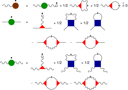
Figure 1: (Color online) Flow diagrams for the one point vertex (1st line) and the self-energies $\Sigma_{hh}$ (2nd line) and $\Sigma_{ab}$. Forcing the one-point vertex to vanish for all $\Lambda$ yields the flow of the order parameter $J_{\Lambda}$.Schuetz06 Wiggly lines correspond to $G_{ab}$ propagators and solid lines to $G_{hh}$. Lines with a dash correspond to single-scale propagators defined via ${\dot{G}}_{ab}=-G_{ab}^{2}\partial_{\Lambda}R_{\Lambda}$ and ${\dot{G}}_{hh}=-G_{hh}^{2}\partial_{\Lambda}R_{\Lambda}$. Small open circles denote the order parameter and the solid dot a derivative with respect to $\Lambda$.

To derive the NPRG equations we expand $\Gamma_{\Lambda}$ in the fields $\Delta{\bm{m}}_{a}=(\partial_{a}{\bm{u}},\partial_{a}h)$. The Dyson equation for the Greens function $G_{hh}$ of the $h$ field, defined via $\big{<}h_{\bm{q}}h_{-{\bm{q}}^{\prime}}\big{>}=V\delta_{{\bm{q}},{\bm{q}^{\prime}}}G_{hh}(q)$ where $V$ is the $D$-dimensional volume, is

$$G_{hh}^{-1}(q)=G_{0,\Lambda}^{-1}(q)+\Sigma_{hh}(q)$$ (5)

with (here and below we suppress in our notation the $\Lambda$ dependence of the coupling parameters)

$$\Sigma_{hh}(q) = ({\tilde{\kappa}}_{q}-{\tilde{\kappa}}_{\Lambda_{0}})q^{4},$$ (6a)

$$G_{0,\Lambda}^{-1} = {\tilde{\kappa}}_{\Lambda_{0}}q^{4}+R_{\Lambda}(q),$$ (6b)

where ${\tilde{\kappa}}_{\Lambda_{0}}$ denotes the bare and momentum independent value of the initial coupling constant ${\tilde{\kappa}}$ defined at the UV cutoff $\Lambda_{0}$. The Greens functions of the in-plane modes, defined via $\big{<}u^{a}_{\bm{k}}u^{b}_{-{\bm{k}}^{\prime}}\big{>}=V\delta_{{\bm{k}},{\bm{k}}^{\prime}}G_{ab}({\bm{k}})$, can be written in terms of transverse and longitudinal components,

$$G_{ab}({\bm{k}})=G_{\perp}(k)\left(\delta_{ab}-k^{a}k^{b}/k^{2}\right)+G_{\parallel}(k)k^{a}k^{b}/k^{2}$$ (7)

with $G_{\alpha}^{-1}=G_{0,\Lambda}^{-1}+\Sigma_{\alpha}$ for $\alpha=\perp,\parallel$, and

$$\Sigma_{\perp}(k) = J^{2}{\tilde{\mu}}_{k}k^{2}+({\tilde{\kappa}}_{k}-{\tilde{\kappa}}_{\Lambda_{0}})k^{4},$$ (8a)

$$\Sigma_{\parallel}(k) = J^{2}(2{\tilde{\mu}}_{k}+{\tilde{\lambda}}_{k})k^{2}+({\tilde{\kappa}}_{k}-{\tilde{\kappa}}_{\Lambda_{0}})k^{4}.$$ (8b)

To determine the flow of $J_{\Lambda}$ and the self-energies, we further need the three and four point vertices. In a symmetrized form they read

$$\Gamma^{(3)}_{abc}(\bm{k}_{1},\bm{k}_{2},\bm{k}_{3}) = -iJ\Big{\{}\tilde{\lambda}_{k_{3}}(\bm{k}_{1}\cdot\bm{k}_{2})k_{3}^{c}\delta_{ab}+\tilde{\lambda}_{k_{2}}(\bm{k}_{1}\cdot\bm{k}_{3})k_{2}^{b}\delta_{ac}+\tilde{\lambda}_{k_{1}}(\bm{k}_{2}\cdot\bm{k}_{3})k_{1}^{a}\delta_{bc}+(\bm{k}_{1}\cdot\bm{k}_{2})(\tilde{\mu}_{k_{1}}k_{3}^{a}\delta_{bc}+\tilde{\mu}_{k_{2}}k_{3}^{b}\delta_{ac})$$ (9a)

$$+(\bm{k}_{1}\cdot\bm{k}_{3})(\tilde{\mu}_{k_{1}}k_{2}^{a}\delta_{bc}+\tilde{\mu}_{k_{3}}k_{2}^{c}\delta_{ab})+(\bm{k}_{2}\cdot\bm{k}_{3})(\tilde{\mu}_{k_{2}}k_{1}^{b}\delta_{ac}+\tilde{\mu}_{k_{3}}k_{1}^{c}\delta_{ab})\Big{\}},$$

$$\Gamma^{(3)}_{hha}(\bm{q}_{1},\bm{q}_{2};\bm{k}) = -iJ\Big{\{}\tilde{\mu}_{k}\big{[}(\bm{q}_{1}\cdot\bm{k})q_{2}^{a}+(\bm{q}_{2}\cdot\bm{k})q_{1}^{a}\big{]}+\tilde{\lambda}_{k}(\bm{q}_{1}\cdot\bm{q}_{2})k^{a}\Big{\}},$$ (9b)

$$\Gamma^{(4)}_{abcd}(\bm{k}_{1},\bm{k}_{2},\bm{k}_{3},\bm{k}_{4}) = \tilde{\mu}_{k_{12}}[(\bm{k}_{1}\cdot\bm{k}_{3})(\bm{k}_{2}\cdot\bm{k}_{4})+(\bm{k}_{1}\cdot\bm{k}_{4})(\bm{k}_{2}\cdot\bm{k}_{3})]\delta_{ab}\delta_{cd}+\tilde{\mu}_{k_{13}}[(\bm{k}_{1}\cdot\bm{k}_{2})(\bm{k}_{3}\cdot\bm{k}_{4})+(\bm{k}_{1}\cdot\bm{k}_{4})(\bm{k}_{2}\cdot\bm{k}_{3})]\delta_{ac}\delta_{bd}$$ (9c)

$$+\tilde{\mu}_{k_{14}}[(\bm{k}_{1}\cdot\bm{k}_{2})(\bm{k}_{3}\cdot\bm{k}_{4})+(\bm{k}_{1}\cdot\bm{k}_{3})(\bm{k}_{2}\cdot\bm{k}_{4})]\delta_{ad}\delta_{bc}$$

$$+\tilde{\lambda}_{k_{12}}(\bm{k}_{1}\cdot\bm{k}_{2})(\bm{k}_{3}\cdot\bm{k}_{4})\delta_{ab}\delta_{cd}+\tilde{\lambda}_{k_{13}}(\bm{k}_{1}\cdot\bm{k}_{3})(\bm{k}_{2}\cdot\bm{k}_{4})\delta_{ac}\delta_{bd}+\tilde{\lambda}_{k_{14}}(\bm{k}_{1}\cdot\bm{k}_{4})(\bm{k}_{2}\cdot\bm{k}_{3})\delta_{ad}\delta_{bc},$$

$$\Gamma^{(4)}_{hhab}(\bm{q}_{1},\bm{q}_{2};\bm{k}_{1},\bm{k}_{2}) = \delta_{ab}\Big{\{}\tilde{\mu}_{q_{12}}\big{[}(\bm{q}_{1}\cdot\bm{k}_{1})(\bm{q}_{2}\cdot\bm{k}_{2})+(\bm{q}_{1}\cdot\bm{k}_{2})(\bm{q}_{2}\cdot\bm{k}_{1})\big{]}+\tilde{\lambda}_{q_{12}}(\bm{q}_{1}\cdot\bm{q}_{2})(\bm{k}_{1}\cdot\bm{k}_{2})\Big{\}}\,,$$ (9d)

$$\Gamma^{(4)}_{hhhh}(\bm{q}_{1},\bm{q}_{2},\bm{q}_{3},\bm{q}_{4}) = (\tilde{\mu}_{q_{12}}+\tilde{\mu}_{q_{14}}+\tilde{\lambda}_{q_{13}})(\bm{q}_{1}\cdot\bm{q}_{3})(\bm{q}_{2}\cdot\bm{q}_{4})+(\tilde{\mu}_{q_{12}}+\tilde{\mu}_{q_{13}}+\tilde{\lambda}_{q_{14}})(\bm{q}_{1}\cdot\bm{q}_{4})(\bm{q}_{2}\cdot\bm{q}_{3})$$ (9e)

$$+(\tilde{\mu}_{q_{13}}+\tilde{\mu}_{q_{14}}+\tilde{\lambda}_{q_{12}})(\bm{q}_{1}\cdot\bm{q}_{2})(\bm{q}_{3}\cdot\bm{q}_{4}),$$

where $k_{ij}=|{\bm{k}}_{i}+{\bm{k}}_{j}|$. The subscript $h$ and momenta ${\bm{q}}_{i}$ refer to $h$ fields while subscripts $a\dots d$ and ${\bm{k}}_{i}$ refer to ${\bm{u}}$ fields. The flow equations for the order parameter $J$ and the self-energies $\Sigma_{hh}$, $\Sigma_{\perp}$, and $\Sigma_{\parallel}$ are rather long and shown diagrammatically in Fig. 1. They yield coupled integro-differential equations for the flow of the coupling functions which must be solved self-consistently. Note that the equations are closed, since all three- and four-point vertices in Eqs. (9a-9e) are entirely determined by coupling functions which can be extracted from the self-energies. This is a result of the form of $\Gamma_{\Lambda}$ in Eqs. (4a,4b) which relates the third and fourth order vertices to lower order ones which in a usual field expansion would have to be imposed through Ward identities.

We integrate the flow equations from the UV cutoff $\Lambda=\Lambda_{0}$ to $\Lambda=0$ numerically, using for numerical stability an analytic regulator, $R_{\Lambda}(q)={\tilde{\kappa}}_{q=0}\,q^{4}/(\exp[(q/\Lambda)^{4}]-1)$ (this one, as well as a non-analytic regulator, were also used in Kownacki09 ). If we ignore the momentum dependence of ${\tilde{\kappa}}_{q}$, ${\tilde{\mu}}_{q}$, and ${\tilde{\lambda}}_{q}$ our flow equations reduce to those reported in Ref. [Kownacki09, ]. In the flat phase we find for $D=2$ $\eta\approx 0.85$ which agrees with the derivative expansion result Kownacki09 . For completeness, we note that our NPRG approach yields for $D=2$ a second order crumpling transition (to within numerical accuracy) with an anomalous dimension $\eta\approx 0.64(5)$, slightly larger than the result $\eta\approx 0.627$ obtained with a sharp cutoff and a derivative expansion in Kownacki09 , where a weak dependence of the flow on the form of the regulator prevented a firm conclusion on the order of the transition. Our result, obtained with a smooth regulator, resolves this ambiguity in favor of a transition of second order. However, we cannot rule out that terms of higher order in the stress tensor would change the nature of the transition.

IV Comparison with MC data and the role of the Ginzburg scale

The MC data for $G_{hh}$ were obtained from a system of $37888$ C-atoms with an accurate bond order potential LCBOPII and $T=300$ K, see Refs. Fasolino07 ; Los09 ; Zackarchenko09 ; Zackarchenko10 for details. To reduce statistical noise, the out-of-plane distortions $h_{i}$ were obtained by evaluating for each $i$ the average ${\bar{h}}_{i}=(3h_{i}+\sum_{\left<i,j\right>}h_{j})/6$ where the sum runs over the three neighbors of atom $i$.Zackarchenko10 As expected, for small $q$ one finds the relation $q^{2}G_{hh}\simeq G_{N}$ between the correlation function of the normals and the height fluctuation which for graphene is extremely accurate even up to $q\approx 1\,{\text{\AA}}^{-1}$, see the inset in Fig. 2. Since the very small $q$ data for $G_{hh}$ is more noisy than that of $G_{N}$ we used for the last three data points ($q<0.07\,{\text{\AA}}^{-1}$) the data of $G_{N}$ to calculate $G_{hh}$, the result is shown in Fig. 2. The strong peak near $q_{B}=4\pi/{3a}\simeq 2.94\,{\text{\AA}}^{-1}$, where $a$ is the equilibrium lattice parameter, corresponds to the first Bragg peak. It defines the upper limit beyond which continuum theory is inapplicable and it serves as a natural UV cutoff for the NPRG calculation, $\Lambda_{0}=q_{B}$. For smaller $q$ the data shows the scaling $G_{hh}\propto q^{-4}$ of the perturbative regime and for very small $q$ the anomalous scaling $G_{hh}\propto q^{-4+\eta}$ where $\eta\approx 0.85$ agrees with the NPRG result.

An important scale is the Ginzburg scale $q_{G}$ for the crossover from the perturbative to the anomalous regime. This scale cannot be captured within a finite order derivative expansion. Perturbation theory membranebook ; Nelson87 yields for $D=2$ the rough estimate

$$q_{G}^{pt}\approx[3\tilde{K}_{0}/(2\pi)]^{1/2}/(4{\tilde{\kappa}})$$ (10)

with $\tilde{K}_{0}=4J^{2}{\tilde{\mu}}({\tilde{\mu}}+{\tilde{\lambda}})/(2{\tilde{\mu}}+{\tilde{\lambda}})$. Below we extract $q_{G}$ from the numerical flow which gives a more accurate estimate.

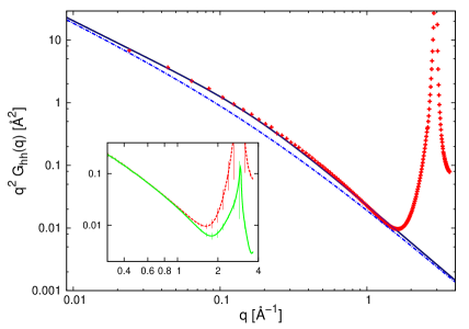
Figure 2: (Color online) Results for the out-of-plane fluctuations $q^{2}G_{hh}(q)$ from NPRG (solid, black), MC (dashed, red) and from a simple phenomenological approximation discussed in the main text (dashed-dotted, blue). The inset shows MC data for the out-of-plane correlations $q^{2}G_{hh}(q)$ (dashed, red) and the fluctuations of normals $G_{N}(q)$ (solid, green).

The RG equations require the initial form of $\tilde{\kappa}_{q},\tilde{\mu}_{q},\tilde{\lambda}_{q}$ and the mean-field order parameter $J_{\Lambda_{0}}$ which are defined at the UV cutoff $\Lambda_{0}$. While we cannot rule out a $q$ dependence of the initial coupling functions, for simplicity and in accordance with Eqs. (1a, 1b) we choose $q$-independent constant values for the initial form of the coupling functions. To fix the initial value of $\kappa$ we use a value previously reported in the literature, $\kappa=1.1\,$eV.Fasolino07 ; Los09 The elastic properties were studied in detail in Ref. [Zackarchenko09, ] and values for the bulk modulus $B=J^{2}(\mu+\lambda)$ and the shear modulus, in our notation $J^{2}\mu$, were extracted for moderate system sizes. For scales smaller than the Ginzburg scale, all elastic constants are strongly cutoff dependent and in particular in the IR limit ${\tilde{\lambda}}_{q=0}$ and ${\tilde{\mu}}_{q=0}$ vanish as $\Lambda^{4-D-2\eta}$ whereas ${\tilde{\kappa}}_{q=0}$ diverges as $\Lambda^{-\eta}$. Values of the elastic constants of free standing graphene must therefore be understood as valid only for a given system size (or IR cutoff). The system size used in Ref. [Zackarchenko09, ] are for $T=300$ K at the border of the perturbative regime and the reported elastic constants are not yet strongly renormalized and close to those at smaller scales. We therefore use these results to fix the initial values of $J^{2}\mu\approx 9.95\,{\rm eV}\,{\text{\AA}}^{-2}$ and $J^{2}\lambda\approx 2.41\,{\rm eV}\,{\text{\AA}}^{-2}$. The initial value of the order parameter $J_{\Lambda_{0}}^{2}\approx 2.5$ is chosen to give the best overall agreement with the MC data. These values place graphene well inside the flat phase, in accordance with numerical simulations which show no sign of crumpling even at high temperatures Fasolino07 . The NPRG result for $G_{hh}$ with these values and $T=300$ K is shown in Fig. 2. The agreement with the MC data is very good, especially the sharpness of the crossover from the perturbative to the anomalous regime is well reproduced. A simple phenomenological ansatz for the self-energy, $\Sigma_{hh}={\tilde{\kappa}}_{\Lambda_{0}}A\,q^{4}(q_{G}/q)^{\eta}$ with $A$ fixed by the asymptotic behavior, does not lead to a satisfactory description of the data, as was already noted in Ref. [Los09, ], see Fig. 2. The Ginzburg scale is by standard definition the scale where selfenergy correction to $\tilde{\kappa}_{q=0}$ equal the bare parameter which allows to read $q_{G}\approx 0.08\,{\text{\AA}}^{-1}$ directly off the flow, which is slightly smaller than the perturbative estimate $q_{G}^{pt}\approx 0.12\,{\text{\AA}}^{-1}$ from Eq. (10). The Ginzburg length $L_{G}=2\pi/q_{G}\approx 80\,{\text{\AA}}$ is of the same order as experimentally observed ripples Meyer07 which offers a natural explanation of their appearance as just the real-space manifestation of the Ginzburg scale. Furthermore, experimentally the fluctuations were found to be broadly distributed around a characteristic scale, which is again in accordance with the behavior of $G_{h}$ around $q_{G}$ which is not characterized by a sharp feature at $q_{G}$ but by a gradual crossover from the perturbative to the anomalous regime. The qualitatively correct perturbative estimate of the Ginzburg scale Eq. (10) furthermore yields a simple dependence of the Ginzburg scale on the temperature, $q_{G}\sim\sqrt{K_{0}k_{B}T}/\kappa$. If our interpretation of ripples in free standing graphene is correct, the average real space scale of ripples should thus increase as $\kappa/\sqrt{K_{0}k_{B}T}$ on lowering the temperature, where $K_{0}$ is the two dimensional Young’s modulus.

V Conclusions

In summary, we have presented a NPRG analyis for tethered membranes which avoids a derivative expansion and is the first to include the full momentum dependence of the elastic coupling parameters. Our solution of the NPRG flow equations is completely self-consistent and obeys all symmetry constraints. In our approach the crumpling transtion is found to be of second order and we give an improved estimate for the anomalous dimension at the transition. For the flat phase of the membrane, we find excellent agreement with MC results for the momentum dependence of the out-of-plane fluctuations of free standing graphene. Also the crossover region, which shows a relatively sharp crossover from the perturbative regime to the anomalous scaling regime which is characterized by a large anomalous dimension, is well reproduced. This strongly supports the notion that free standing graphene behaves just as a tethered membrane, albeit a very stiff one. The most important scale in the analysis of the momentum dependence of the membrane fluctuations is the Ginzburg scale which we find to be of the same order as the experimentally determined characteristic size of ripples. The observation of ripples at this scale should thus be looked at as a confirmation of the continuum elastic theory of tethered membranes, a notion which could also be tested experimentally by measuring the characteristic ripple scale as a funtion of temperature.

We thank Annalisa Fasolino, Jan H. Los, Konstantin Zakharchenko, and Misha Katsnelson for discussions and sharing their MC data with us prior to publication. We further thank Antonio H. Castro Neto and Dominique Mouhanna for discussions.

References

- (1) See A. H. Castro Neto, F. Guinea, N. M. R. Peres, K. S. Novoselov, and A. K. Geim, Rev. Mod. Phys 81, 109 (2009) for a recent review.
- (2) D. R. Nelson, T. Piran, and S. Weinberg (Eds.), Statistical Mechanics of Membranes and Surfaces, 2nd edition, World Scientific, Singapore (2004).
- (3) J. H. Los, M. I. Katsnelson, O. V. Yazyev, K. V. Zakharchenko, and A. Fasolino, Phys. Rev. B 80, 121405(R) (2009).
- (4) J. C. Meyer, A. K. Geim, M. I. Katsnelson, K. S. Novoselov, T. J. Booth, and S. Roth, Nature 446, 60 (2007).
- (5) A. Fasolino, J. H. Los, and M. I. Katsnelson, Nature Mater. 6, 858 (2007).
- (6) D. Gazit, Phys. Rev. B 80, 161406(R) (2009).
- (7) D. R. Nelson and L. Peliti, J. Phys. (Paris) 48, 1085 (1987).
- (8) M. Paczuski, M. Kardar, and D. R. Nelson, Phys. Rev. Lett. 60, 2638 (1988).
- (9) J. Aronovitz, L. Golubović, and T. C. Lubensky, J. Phys. (Paris) 50, 609 (1989).
- (10) P. Le Doussal and L. Radzihovsky, Phys. Rev. Lett. 69, 1209 (1992).
- (11) D. Gazit, Phys. Rev. E 80, 041117 (2009).
- (12) J. P. Kownacki and D. Mouhanna, Phys. Rev. E 79, 040101(R) (2009).
- (13) J. A. Aronovitz and T. C. Lubensky, Phys. Rev. Lett. 60, 2634 (1988).
- (14) C. Wetterich, Phys. Lett. B 301, 90 (1993); T. R. Morris, Int. J. Mod. Phys. A 9, 2411 (1994).
- (15) F. Schütz and P. Kopietz, J. Phys. A 39, 8205 (2006).
- (16) K. V. Zakharchenko, M. I. Katsnelson, and A. Fasolino, Phys. Rev. Lett. 102, 046808 (2009).
- (17) K. V. Zakharchenko, J. H. Los, M. I. Katsnelson, and A. Fasolino, arXiv:1004.0126.