A fuller flavour treatment of $N_{2}$-dominated leptogenesis

Abstract

We discuss $N_{2}$-dominated leptogenesis in the presence of flavour dependent effects that have hitherto been neglected, in particular the off-diagonal entries of the flavour coupling matrix that connects the total flavour asymmetries, distributed in different particle species, to the lepton and Higgs doublet asymmetries. We derive analytical formulae for the final asymmetry including the flavour coupling at the $N_{2}$-decay stage as well as at the stage of washout by the lightest right-handed neutrino $N_{1}$. Moreover, we point out that in general part of the electron and muon asymmetries (phantom terms), can completely escape the wash-out at the production and a total $B-L$ asymmetry can be generated by the lightest RH neutrino wash-out yielding so called phantom leptogenesis. However, the phantom terms are proportional to the initial $N_{2}$ abundance and in particular they vanish for initial zero $N_{2}$-abundance. Taking any of these new effects into account can significantly modify the final asymmetry produced by the decays of the next-to-lightest RH neutrinos, opening up new interesting possibilities for $N_{2}$-dominated thermal leptogenesis.

1 Introduction

Leptogenesis [1] is based on a popular extension of the Standard Model, where three right-handed (RH) neutrinos $N_{Ri}$, with a Majorana mass term $M$ and Yukawa couplings $h$, are added to the SM Lagrangian,

$$\mathcal{L}=\mathcal{L}_{\rm SM}+i\overline{N}_{Ri}\gamma_{\mu}\partial^{\mu}N_{Ri}-h_{\alpha i}\overline{\ell}_{L\alpha}N_{Ri}\tilde{\Phi}-{1\over 2}\,M_{i}\overline{N}_{Ri}^{c}\,N_{Ri}+h.c.\quad(i=1,2,3,\quad\alpha=e,\mu,\tau)\,.$$ (1)

After spontaneous symmetry breaking, a Dirac mass term $m_{D}=v\,h$, is generated by the vev $v=174$ GeV of the Higgs boson. In the see-saw limit, $M\gg m_{D}$, the spectrum of neutrino mass eigenstates splits in two sets: 3 very heavy neutrinos $N_{1},N_{2}$ and $N_{3}$, respectively with masses $M_{1}\leq M_{2}\leq M_{3}$, almost coinciding with the eigenvalues of $M$, and 3 light neutrinos with masses $m_{1}\leq m_{2}\leq m_{3}$, the eigenvalues of the light neutrino mass matrix given by the see-saw formula [2]

$$m_{\nu}=-m_{D}\,{1\over M}\,m_{D}^{T}\,.$$ (2)

Neutrino oscillation experiments measure two neutrino mass-squared differences. For normal schemes one has $m^{\,2}_{3}-m_{2}^{\,2}=\Delta m^{2}_{\rm atm}$ and $m^{\,2}_{2}-m_{1}^{\,2}=\Delta m^{2}_{\rm sol}$, whereas for inverted schemes one has $m^{\,2}_{3}-m_{2}^{\,2}=\Delta m^{2}_{\rm sol}$ and $m^{\,2}_{2}-m_{1}^{\,2}=\Delta m^{2}_{\rm atm}$. For $m_{1}\gg m_{\rm atm}\equiv\sqrt{\Delta m^{2}_{\rm atm}+\Delta m^{2}_{\rm sol}}=(0.050\pm 0.001)\,{\rm eV}$ [3] the spectrum is quasi-degenerate, while for $m_{1}\ll m_{\rm sol}\equiv\sqrt{\Delta m^{2}_{\rm sol}}=(0.0088\pm 0.0001)\,{\rm eV}$ [3] it is fully hierarchical (normal or inverted). The most stringent upper bound on the absolute neutrino mass scale comes from cosmological observations. Recently, quite a conservative upper bound,

$$m_{1}<0.2\,{\rm eV}\,\hskip 14.22636pt(95\%\,{\rm CL})\,,$$ (3)

has been obtained by the WMAP collaboration combining CMB, baryon acoustic oscillations and supernovae type Ia observations [4].

The $C\!P$ violating decays of the RH neutrinos into lepton doublets and Higgs bosons at temperatures $T\gtrsim 100\,{\rm GeV}$ generate a $B-L$ asymmetry one third of which, thanks to sphaleron processes, ends up into a baryon asymmetry that can explain the observed baryon asymmetry of the Universe. This can be expressed in terms of the baryon-to-photon number ratio and a precise measurement comes from the CMBR anisotropies observations of WMAP [4],

$$\eta_{B}^{\rm CMB}=(6.2\pm 0.15)\times 10^{-10}\,.$$ (4)

The predicted baryon-to-photon ratio $\eta_{B}$ is related to the final value of the $(B-L)$ asymmetry $N^{\rm f}_{B-L}$ by the relation

$$\eta_{B}\simeq 0.96\times 10^{-2}N_{B-L}^{\rm f}\,,$$ (5)

where we indicate with $N_{X}$ any particle number or asymmetry $X$ calculated in a portion of co-moving volume containing one heavy neutrino in ultra-relativistic thermal equilibrium, so that e.g. $N^{\rm eq}_{N_{2}}(T\gg M_{2})=1$.

If one imposes that the RH neutrino mass spectrum is strongly hierarchical, then there are two options for successful leptogenesis. A first one is given by the $N_{1}$-dominated scenario, where the final asymmetry is dominated by the decays of the lightest RH neutrinos. The main limitation of this scenario is that successful leptogenesis implies quite a restrictive lower bound on the mass of the lightest RH neutrino. Imposing independence of the final asymmetry of the initial RH neutrino abundance and barring phase cancelations in the see-saw orthogonal matrix entries the lower bound is given by [5, 6, 7]

$$M_{1}\gtrsim 3\times 10^{9}\,{\rm GeV}\,.$$ (6)

This implies in turn a lower bound $T_{\rm reh}\gtrsim 1.5\times 10^{9}\,{\rm GeV}$ on the reheating temperature as well [8] . The lower bound Eq. (6) is typically not respected in models emerging from grand unified theories. It has therefore been long thought that, within a minimal type I see-saw mechanism, leptogenesis is not viable within these models [11].

There is however a second option [12], namely the $N_{2}$-dominated leptogenesis scenario, where the asymmetry is dominantly produced from the decays of the next-to-lightest RH neutrinos. In this case there is no lower bound on the lightest RH neutrino mass $M_{1}$. Instead this is replaced by a lower bound on the next-to-lightest RH neutrino mass $M_{2}$ that still implies a lower bound on the reheating temperature.

There are two necessary conditions for a successful $N_{2}$-dominated leptogenesis scenario. The first one is the presence of (at least) a third heavier RH neutrino $N_{3}$ that couples to $N_{2}$ in order for the $C\!P$ asymmetries of $N_{2}$ not to be suppressed as $\propto(M_{1}/M_{2})^{2}$. The second necessary condition is to be able to circumvent the wash-out from the lightest RH neutrinos. There is a particular choice of the see-saw parameters where these two conditions are maximally satisfied. This corresponds to the limit where the lightest RH neutrino gets decoupled, as in heavy sequential dominance, an example which we shall discuss later. In this case the bound, $M_{2}\gtrsim 10^{10}\,{\rm GeV}$ when estimated without the inclusion of flavour effects, is saturated. In this limit the wash-out from the lightest RH neutrinos is totally absent and the $C\!P$ asymmetries of the $N_{2}$’s are maximal.

In order to have successful $N_{2}$-dominated leptogenesis for choices of the parameters not necessarily close to this maximal case a crucial role is played by lepton flavour effects [13]. If $M_{1}\ll 10^{9}\,{\rm GeV}\ll M_{2}$, as we will assume, then before the lightest RH neutrino wash-out is active, the quantum states of the lepton doublets produced by $N_{2}$-decays get fully incoherent in flavour space [15, 14, 16, 17, 18]. In this way the lightest RH neutrino wash-out acts separately on each flavour asymmetry and is then much less efficient [13] . It has then been shown recently that within this scenario it is possible to have successful leptogenesis within models emerging from $SO(10)$ grand-unified theories with interesting potential predictions on the low energy parameters [21]. Therefore, the relevance of the $N_{2}$-dominated scenario has been gradually increasing in the last years.

In this paper we discuss $N_{2}$-dominated leptogenesis in the presence of flavour dependent effects that have hitherto been neglected, in particular the off-diagonal entries of the flavour coupling matrix that connects the total flavour asymmetries, distributed in different particle species, to the lepton and Higgs doublet asymmetries. We derive analytical formulae for the final asymmetry including the flavour coupling at the $N_{2}$-decay stage as well as at the stage of washout by the lightest RH neutrino $N_{1}$. We point out that in general part of the electron and muon asymmetries will completely escape the wash-out at the production and a total $B-L$ asymmetry can be generated by the lightest RH neutrino wash-out yielding so called phantom leptogenesis. These contributions, that we call phantom terms, introduce however a strong dependence on the initial conditions as we explain in detail. Taking of all these new effects into account can enhance the final asymmetry produced by the decays of the next-to-lightest RH neutrinos by orders of magnitude, opening up new interesting possibilities for $N_{2}$-dominated thermal leptogenesis. We illustrate these effects for two models which describe realistic neutrino masses and mixing based on sequential dominance.

The layout of the remainder of the paper is as follows. In section 2 we discuss the production of the asymmetry from $N_{2}$-decays and its subsequent thermal washout at similar temperatures. In section 3 we discuss three flavour projection and the wash-out stage at lower temperatures relevant to the lightest RH neutrino mass. This is where the asymmetry which survives from $N_{2}$-decays and washout would typically be expected to be washed out by the lightest RH neutrinos in a flavour independent treatment, but which typically survives in a flavour-dependent treatment. This conclusion is reinforced in the fuller flavour treatment here making $N_{2}$ dominated leptogenesis even more relevant. The fuller flavour effects of the $N_{2}$-dominated scenario are encoded in a compact master formula presented at the end of this section and partly unpacked in an Appendix. Section 4 applies this master formula to examples where the new effects arising from the flavour couplings and phantom leptogenesis play a prominent role. We focus on examples where, due to the considered effects, the flavour asymmetry produced dominantly in one flavour can emerge as an asymmetry in a different flavour, a scenario we refer to as the flavour swap scenario.

2 Production of the asymmetry from $N_{2}$-decays and washout

In the $N_{2}$-dominated scenario, with $M_{2}$ respecting the lower bound of $M_{2}\gtrsim 10^{10}\,{\rm GeV}$ and $M_{1}\ll 10^{9}\,{\rm GeV}$, one has to distinguish two stages in the calculation of the asymmetry. In a first production stage, at $T\simeq T_{L}\sim M_{2}$, a $B-L$ asymmetry is generated from the $N_{2}$ decays. In a second wash-out stage, at $T\sim M_{1}$, inverse processes involving the lightest RH neutrinos, the $N_{1}$’s, become effective and wash-out the asymmetry to some level.

In the production stage, since we assume $10^{12}\,{\rm GeV}\gg M_{2}\gg 10^{9}\,{\rm GeV}$, the $B-L$ asymmetry is generated from the $N_{2}$-decays in the so called two-flavour regime [14, 15, 16]. In this regime the $\tau$-Yukawa interactions are fast enough to break the coherent evolution of the tauon component of the lepton quantum states between a decay and the subsequent inverse decay and light flavour effects have to be taken into account in the calculation of the final asymmetry. On the other hand the evolution of the muon and of the electron components superposition is still coherent.

If we indicate with $|\ell_{2}\rangle$ the quantum state describing the leptons produced by $N_{2}$-decays, we can define the flavour branching ratios giving the probability $P_{2\alpha}$ that $|\ell_{2}\rangle$ is measured in a flavour eigenstate $|\ell_{\alpha}\rangle$ as $P_{2\alpha}\equiv|\langle\ell_{\alpha}|\ell_{2}\rangle|^{2}$. Analogously, indicating with $|\bar{\ell}_{2}^{\prime}\rangle$ the quantum state describing the anti-leptons produced by $N_{2}$-decays, we can define the anti-flavour branching ratios as $\bar{P}_{2\alpha}\equiv|\langle\bar{\ell}_{\alpha}|\bar{\ell}^{\prime}_{2}\rangle|^{2}$. The tree level contribution is simply given by the average $P^{0}_{2\alpha}=(P_{2\alpha}+\bar{P}_{2\alpha})/2$. The total decay width of the $N_{2}$’s can be expressed in terms of the Dirac mass matrix as

$$\widetilde{\Gamma}_{2}={M_{2}\over 8\,\pi\,v^{2}}\,(m^{\dagger}_{D}\,m_{D})_{22}$$ (7)

and is given by the sum $\widetilde{\Gamma}_{2}=\Gamma_{2}+\bar{\Gamma}_{2}$ of the total decay rate into leptons and of the total decay rate into anti-leptons respectively. The flavoured decay widths are given by

$$\widetilde{\Gamma}_{2\alpha}={M_{2}\over 8\,\pi\,v^{2}}\,|m_{D\alpha 2}|^{2}\,,$$ (8)

and can be also expressed as a sum, $\widetilde{\Gamma}_{2\alpha}=\Gamma_{2\alpha}+\bar{\Gamma}_{2\alpha}$, of the flavoured decay rate into leptons and of the flavoured total decay rate into anti-leptons respectively.

Notice that the branching ratios can then be expressed in terms of the rates as $P_{2\alpha}=\Gamma_{2\alpha}/\Gamma_{2}$ and $\bar{P}_{2\alpha}=\bar{\Gamma}_{2\alpha}/\bar{\Gamma}_{2}$. The flavoured $C\!P$ asymmetries for the $N_{2}$-decays into $\alpha$-leptons ($\alpha=e,\mu,\tau$) are then defined as

$$\varepsilon_{2\alpha}\equiv-\,{\Gamma_{2\alpha}-\overline{\Gamma}_{2\alpha}\over\Gamma_{2}+\overline{\Gamma}_{2}}\,,$$ (9)

while the total $C\!P$ asymmetries as

$$\varepsilon_{2}\equiv-\,{\Gamma_{2}-\bar{\Gamma}_{2}\over\Gamma_{2}+\bar{\Gamma}_{2}}=\sum_{\alpha}\varepsilon_{2\alpha}\,.$$ (10)

The three flavoured $C\!P$ asymmetries can be calculated using [22]

$$\varepsilon_{2\alpha}=\frac{3}{16\pi(h^{{\dagger}}h)_{22}}\sum_{j\neq 2}\left\{{\rm Im}\left[h_{\alpha 2}^{\star}h_{\alpha j}(h^{{\dagger}}h)_{2j}\right]\frac{\xi(x_{j})}{\sqrt{x_{j}}}+\frac{2}{3(x_{j}-1)}{\rm Im}\left[h_{\alpha 2}^{\star}h_{\alpha j}(h^{{\dagger}}h)_{j2}\right]\right\}\,,$$ (11)

where $x_{j}\equiv(M_{j}/M_{2})^{2}$ and

$$\xi(x)={2\over 3}\,x\,\left[(1+x)\,\ln\left({1+x\over x}\right)-{2-x\over 1-x}\right]\,.$$ (12)

The tree-level branching ratios can then be expressed as

$$P^{0}_{2\alpha}={\widetilde{\Gamma}_{2\alpha}\over\widetilde{\Gamma}_{2}}+{\cal O}(\varepsilon^{2})\simeq{|m_{D\alpha 2}|^{2}\over(m^{\dagger}_{D}\,m_{D})_{22}}\,.$$ (13)

Defining $\Delta P_{2\alpha}\equiv P_{2\alpha}-\bar{P}_{2\alpha}$, it will prove useful to notice that the flavoured asymmetries can be decomposed as the sum of two terms [15],

$$\varepsilon_{2\alpha}=P^{0}_{2\alpha}\,\varepsilon_{2}-{\Delta P_{2\alpha}\over 2}\,,$$ (14)

where the first term is due to an imbalance between the total number of produced leptons and anti-leptons and is therefore proportional to the total $C\!P$ asymmetry, while the second originates from a different flavour composition of the lepton quantum states with respect to the $C\!P$ conjugated anti-leptons quantum states.

Sphaleron processes conserve the flavoured asymmetries $\Delta_{\alpha}\equiv B/3-L_{\alpha}$ ($\alpha=e,\mu,\tau$). Therefore, the Boltzmann equations are particularly simple in terms of these quantities [19]. In the two-flavour regime the electron and the muon components of $|{\ell}_{2}\rangle$ evolve coherently and the wash-out from inverse processes producing the $N_{2}$’s acts then on the sum $N_{\Delta_{\gamma}}\equiv N_{\Delta_{e}}+N_{\Delta_{\mu}}$. Therefore, it is convenient to define correspondingly $P^{0}_{2\gamma}\equiv P^{0}_{2e}+P^{0}_{2\mu}$ and $\varepsilon_{2\gamma}\equiv\varepsilon_{2e}+\varepsilon_{2\mu}$. More generally, any quantity with a subscript ‘$\gamma$’ has to be meant as the sum of the same quantity calculated for the electron and for the muon flavour component.

The asymmetry produced by the lightest and by the heaviest RH neutrino decays is negligible since their $C\!P$ asymmetries are highly suppressed with the assumed mass pattern. The set of classic kinetic equations reduces then to a very simple one describing the asymmetry generated by the $N_{2}$-decays,

$${dN_{N_{2}}\over dz_{2}} = -D_{2}\,(N_{N_{2}}-N_{N_{2}}^{\rm eq})\,,$$ (15)

$${dN_{\Delta_{\gamma}}\over dz_{2}} = \varepsilon_{2\gamma}\,D_{2}\,(N_{N_{2}}-N_{N_{2}}^{\rm eq})-P_{2\gamma}^{0}\,W_{2}\,\sum_{\alpha=\gamma,\tau}\,C_{\gamma\alpha}^{(2)}\,N_{\Delta_{\alpha}}\,,$$ (16)

$${dN_{\Delta_{\tau}}\over dz_{2}} = \varepsilon_{2\tau}\,D_{2}\,(N_{N_{2}}-N_{N_{2}}^{\rm eq})-P_{2\tau}^{0}\,W_{2}\,\sum_{\alpha=\gamma,\tau}\,C_{\tau\alpha}^{(2)}\,N_{\Delta_{\alpha}}\,.$$ (17)

where $z_{2}\equiv M_{2}/T$. The total $B-L$ asymmetry can then be calculated as $N_{B-L}=N_{\Delta_{\tau}}+N_{\Delta_{\gamma}}$. The equilibrium abundances are given by $N_{N_{2}}^{\rm eq}=z_{2}^{2}\,{\cal K}_{2}(z_{2})/2$, where we indicated with ${\cal K}_{i}(z_{2})$ the modified Bessel functions. Introducing the total decay parameter $K_{2}\equiv\widetilde{\Gamma}_{2}(T=0)/H(T=M_{2})$, the decay term $D_{2}$ can be expressed as

$$D_{2}(z_{2})\equiv{\widetilde{\Gamma}_{2}\over H\,z}=K_{2}\,z_{2}\,\left\langle{1\over\gamma}\right\rangle\,,$$ (18)

where $\langle 1/\gamma\rangle(z_{2})$ is the thermally averaged dilation factor and is given by the ratios ${\cal K}_{1}(z_{2})/{\cal K}_{2}(z_{2})$. Finally, the inverse decays wash-out term is given by

$$W_{2}(z_{2})={1\over 4}\,K_{2}\,{\cal K}_{1}(z_{2})\,z_{2}^{3}\,.$$ (19)

The total decay parameter $K_{2}$ is related to the Dirac mass matrix by

$$K_{2}={\widetilde{m}_{2}\over m_{\star}}\,,\hskip 28.45274pt{\rm where}\hskip 28.45274pt\widetilde{m}_{2}\equiv{(m_{D}^{\dagger}\,m_{D})_{22}\over M_{2}}$$ (20)

is the effective neutrino mass [23] and $m_{\star}$ is equilibrium neutrino mass defined by [24, 8]

$$m_{\star}\equiv{16\,\pi^{5/2}\,\sqrt{g_{*}}\over 3\,\sqrt{5}}\,{v^{2}\over M_{\rm Pl}}\simeq 1.08\times 10^{-3}\,{\rm eV}.$$ (21)

It will also prove convenient to introduce the flavoured effective neutrino masses $\widetilde{m}_{2\alpha}\equiv P^{0}_{2\alpha}\,\widetilde{m}_{2}$ and correspondingly the flavoured decay parameters $K_{2\alpha}\equiv P^{0}_{2\alpha}\,K_{2}=\widetilde{m}_{2\alpha}/m_{\star}$, so that $\sum_{\alpha}\widetilde{m}_{2\alpha}=\widetilde{m}_{2}$ and $\sum_{\alpha}K_{2\alpha}=K_{2}$.

The flavour coupling matrix $C$ [19, 25, 26, 9, 15, 7] relates the asymmetries stored in the lepton doublets and in the Higgs bosons to the $\Delta_{\alpha}$’s. It is therefore the sum of two contributions,

$$C_{\alpha\beta}=C^{\ell}_{\alpha\beta}+C^{H}_{\alpha\beta}\,,$$ (22)

the first one connecting the asymmetry in the lepton doublets and the second connecting the asymmetry in the Higgs bosons. Flavour dynamics couple because the generation of a leptonic asymmetry into lepton doublets from $N_{i}$ decays is necessarily accompanied by a generation of a hypercharge asymmetry into the Higgs bosons and of a baryonic asymmetry into quarks via sphaleron processes. The asymmetry generated into the lepton doublets is moreover also redistributed to right handed charged particles. The wash-out of a specific flavour asymmetry is then influenced by the dynamics of the asymmetries stored in the other flavours because they are linked primarily through the asymmetry into the Higgs doublets and secondarily through the asymmetry into quarks.

The condition of chemical equilibrium gives a constraint on the chemical potential (hence number density asymmetry) of each such species. Solving for all constraints one obtains the $C_{\alpha\beta}$ explicitly. If we indicate with $C^{(2)}$ the coupling matrix in the two-flavour regime, the two contributions to the flavour coupling matrix are given by

$$C^{l(2)}=\left(\begin{array}[]{ccc}417/589&-120/589\\ -30/589&390/589\end{array}\right)\,\hskip 11.38109pt\mbox{\rm and}\hskip 11.38109ptC^{h(2)}=\left(\begin{array}[]{ccc}164/589&224/589\\ 164/589&224/589\end{array}\right)\,,$$ (23)

and summing one obtains

$$C^{(2)}\equiv\left(\begin{array}[]{ccc}C^{(2)}_{\gamma\gamma}&C^{(2)}_{\gamma\tau}\\ C^{(2)}_{\tau\gamma}&C^{(2)}_{\tau\tau}\end{array}\right)=\left(\begin{array}[]{ccc}581/589&104/589\\ 194/589&614/589\end{array}\right)\,.$$ (24)

A traditional calculation, where flavour coupling is neglected, corresponds to approximating the $C$-matrix by the identity matrix. In this case the evolution of the two flavour asymmetries proceeds uncoupled and they can be easily worked out in an integral form [27, 8, 7],

$$N_{\Delta\alpha}(z_{2})=N_{\Delta\alpha}^{\rm in}\,e^{-P_{2\alpha}^{0}\,\int_{z_{2}^{\rm in}}^{z_{2}}\,dz_{2}^{\prime}\,W_{2}(z_{2}^{\prime})}+\varepsilon_{2\alpha}\,\kappa(z_{2};K_{2\alpha})\,,$$ (25)

where the efficiency factors are given by

$$\kappa(z_{2};K_{2\alpha})=-\int_{z_{2}^{\rm in}}^{z_{2}}\,dz_{2}^{\prime}\,{dN_{N_{i}}\over dz_{2}^{\prime}}\,e^{-P_{2\alpha}^{0}\,\int_{z_{2}^{\prime}}^{z}\,dz_{2}^{\prime\prime}\,W_{2}(z_{2}^{\prime\prime})}\,.$$ (26)

We will neglect the first term due the presence of possible initial flavour asymmetries and assume $z_{2}^{\rm in}\ll 1$. The efficiency factors and therefore the asymmetries get frozen to a particular value of the temperature given by $T_{L\alpha}=M_{2}/z_{B}(K_{2\alpha})$, where [28]

$$z_{B}(K_{2\alpha})\simeq 2+4\,K_{2\alpha}^{0.13}\,e^{-{2.5\over K_{2\alpha}}}={\cal O}(1\div 10)\,.$$ (27)

Defining $T_{L}\equiv{\rm min}(T_{L\tau},T_{L\gamma})$, the total final $B-L$ asymmetry at $T_{L}$ is then given by

$$N_{B-L}^{T\sim T_{L}}\simeq\varepsilon_{2\gamma}\,\kappa(K_{2\gamma})+\varepsilon_{2\tau}\,\kappa(K_{2\tau})\,.$$ (28)

Assuming an initial thermal $N_{2}$-abundance, the final efficiency factors $\kappa(K_{2\alpha})\equiv\kappa(z_{2}=\infty,K_{2\alpha})$ are given approximately by [7]

$$\kappa(K_{2\alpha})\simeq\frac{2}{K_{2\alpha}\,z_{\rm B}(K_{2\alpha})}\left[1-{\rm exp}\left(-\frac{1}{2}K_{2\alpha}\,z_{\rm B}(K_{2\alpha})\right)\right]\,.$$ (29)

On the other hand, in the case of vanishing initial abundances , the efficiency factors are the sum of two different contributions, a negative and a positive one,

$$\kappa_{2\alpha}^{\rm f}=\kappa_{-}^{\rm f}(K_{2},P_{2\alpha}^{0})+\kappa_{+}^{\rm f}(K_{2},P_{2\alpha}^{0})\,.$$ (30)

The negative contribution arises from a first stage where $N_{N_{2}}\leq N_{N_{2}}^{\rm eq}$, for $z_{2}\leq z_{2}^{\rm eq}$, and is given approximately by

$$\kappa_{-}^{\rm f}(K_{2},P_{2\alpha}^{0})\simeq-{2\over P_{2\alpha}^{0}}\ e^{-{3\,\pi\,K_{2\alpha}\over 8}}\left(e^{{P_{2\alpha}^{0}\over 2}\,N_{N_{2}}(z_{\rm eq})}-1\right)\,.$$ (31)

The $N_{2}$-abundance at $z_{2}^{\rm eq}$ is well approximated by the expression

$$N_{N_{2}}(z_{2}^{\rm eq})\simeq\overline{N}(K_{2})\equiv{N(K_{2})\over\left(1+\sqrt{N(K_{2})}\right)^{2}}\,,$$ (32)

that interpolates between the limit $K_{2}\gg 1$, where $z_{2}^{\rm eq}\ll 1$ and $N_{\rm N_{2}}(z_{2}^{\rm eq})=1$, and the limit $K_{2}\ll 1$, where $z_{2}^{\rm eq}\gg 1$ and $N_{N_{2}}(z_{2}^{\rm eq})=N(K_{2})\equiv 3\pi K_{2}/4$. The positive contribution arises from a second stage when $N_{N_{2}}\geq N_{N_{2}}^{\rm eq}$, for $z_{2}\geq z_{2}^{\rm eq}$, and is approximately given by

$$\kappa_{+}^{\rm f}(K_{2},P_{2\alpha}^{0})\simeq{2\over z_{B}(K_{2\alpha})\,K_{2\alpha}}\left(1-e^{-{K_{2\alpha}\,z_{B}(K_{2\alpha})\,N_{N_{2}}(z_{\rm eq})\over 2}}\right)\,.$$ (33)

If flavour coupling is taken into account, we can still solve analytically eqs. (15) performing the following change of variables

$$\left(\begin{array}[]{c}N_{\Delta_{\gamma^{\prime}}}\\ N_{\Delta_{\tau^{\prime}}}\end{array}\right)=U\,\left(\begin{array}[]{c}N_{\Delta_{\gamma}}\\ N_{\Delta_{\tau}}\end{array}\right)\,,\hskip 14.22636pt\mbox{\rm where}\hskip 14.22636ptU\equiv\left(\begin{array}[]{cc}U_{\gamma^{\prime}\gamma}&U_{\gamma^{\prime}\tau}\\ U_{\tau^{\prime}\gamma}&U_{\tau^{\prime}\tau}\end{array}\right)$$ (34)

is the matrix that diagonalizes

$$P^{0}_{2}\equiv\left(\begin{array}[]{cc}P^{0}_{2\gamma}\,C_{\gamma\gamma}^{(2)}&P^{0}_{2\gamma}\,C_{\gamma\tau}^{(2)}\\ P^{0}_{2\tau}\,C_{\tau\gamma}^{(2)}&P^{0}_{2\tau}\,C_{\tau\tau}^{(2)}\end{array}\right)\,,$$ (35)

i.e. $U\,P^{0}_{2}\,U^{-1}={\rm diag}(P^{0}_{2\gamma^{\prime}},P^{0}_{2\tau^{\prime}})$. In these new variables the two kinetic equations for the flavoured asymmetries decouple,

$${dN_{\Delta_{\gamma^{\prime}}}\over dz_{2}} = \varepsilon_{2\gamma^{\prime}}\,D_{2}\,(N_{N_{2}}-N_{N_{2}}^{\rm eq})-P^{0}_{2\gamma^{\prime}}\,W_{2}\,N_{\Delta_{\gamma^{\prime}}}\,$$ (36)

$${dN_{\Delta_{\tau^{\prime}}}\over dz_{2}} = \varepsilon_{2\tau^{\prime}}\,D_{2}\,(N_{N_{2}}-N_{N_{2}}^{\rm eq})-P^{0}_{2\tau^{\prime}}\,W_{2}\,N_{\Delta_{\tau^{\prime}}}\,,$$ (37)

where we defined

$$\left(\begin{array}[]{c}\varepsilon_{2\gamma^{\prime}}\\ \varepsilon_{2\tau^{\prime}}\end{array}\right)\equiv U\,\left(\begin{array}[]{c}\varepsilon_{2\gamma}\\ \varepsilon_{2\tau}\end{array}\right)\,.$$ (38)

The solutions for the two $N_{\Delta_{\alpha^{\prime}}}$ are then still given by eq. (25) where, however, now the ‘unprimed’ quantities have to be replaced with the ‘primed’ quantities and therefore explicitly one has

$$N_{\Delta_{\gamma^{\prime}}}^{T\sim T_{L}} \simeq \varepsilon_{2\gamma^{\prime}}\,\kappa(K_{2\gamma^{\prime}})\,,$$ (39)

$$N_{\Delta_{\tau^{\prime}}}^{T\sim T_{L}} \simeq \varepsilon_{2\tau^{\prime}}\,\kappa(K_{2\tau^{\prime}})\,.$$

Notice that the $B-L$ asymmetry at $T\sim T_{L}$ is still given by $N_{B-L}^{T\sim T_{L}}=N_{\Delta_{\gamma}}^{T\sim T_{L}}+N_{\Delta_{\tau}}^{T\sim T_{L}}$. The two $N_{\Delta_{\alpha}}$’s can be calculated from the two $N_{\Delta_{\alpha^{\prime}}}$’s using the inverse transformation

$$\left(\begin{array}[]{c}N_{\Delta_{\gamma}}^{T\sim T_{L}}\\ N_{\Delta_{\tau}}^{T\sim T_{L}}\end{array}\right)=U^{-1}\,\left(\begin{array}[]{c}N_{\Delta_{\gamma^{\prime}}}^{T\sim T_{L}}\\ N_{\Delta_{\tau^{\prime}}}^{T\sim T_{L}}\end{array}\right)\,,\hskip 14.22636pt\mbox{\rm where}\hskip 14.22636ptU^{-1}\equiv\left(\begin{array}[]{cc}U^{-1}_{\gamma\gamma^{\prime}}&U^{-1}_{\gamma\tau^{\prime}}\\ U^{-1}_{\tau\gamma^{\prime}}&U^{-1}_{\tau\tau^{\prime}}\end{array}\right)\,.$$ (40)

To study the impact of flavour coupling on the final asymmetry, we can calculate the ratio

$$R\equiv\left|{N_{B-L}\over\left.N_{B-L}\right|_{C=I}}\right|$$ (41)

between the asymmetry calculated taking into account flavour coupling, and the asymmetry calculated neglecting flavour coupling, corresponding to the assumption $C=I$. If we want first to calculate the value of $R$ at the production stage, we have to express $N_{B-L}^{T\sim T_{L}}$ in terms of the ‘unprimed’ quantities in eq. (39). This is quite easy for the $K_{2\alpha^{\prime}}$, since one has simply to find the eigenvalues of the matrix $P_{2}^{0}$. Taking for simplicity the approximation $C^{(2)}_{\gamma\gamma}\simeq C^{(2)}_{\tau\tau}\simeq 1$, and remembering that $P_{2\gamma}^{0}+P_{2\tau}^{0}=1$, one obtains

$$P^{0}_{2\gamma^{\prime}} \simeq {1\over 2}\,\left(1+\sqrt{(P^{0}_{2\gamma}-P^{0}_{2\tau})^{2}+4\,C^{(2)}_{\gamma\tau}\,C^{(2)}_{\tau\gamma}\,P^{0}_{2\gamma}\,P^{0}_{2\tau}}\right)\,,$$ (42)

$$P^{0}_{2\tau^{\prime}} \simeq {1\over 2}\,\left(1-\sqrt{(P^{0}_{2\gamma}-P^{0}_{2\tau})^{2}+4\,C^{(2)}_{\gamma\tau}\,C^{(2)}_{\tau\gamma}\,P^{0}_{2\gamma}\,P^{0}_{2\tau}}\right).$$ (43)

Notice that, both for $\alpha=\tau$ and $\alpha=\gamma$, one has $P^{0}_{2\alpha^{\prime}}\simeq P^{0}_{2\alpha}+{\cal O}(\sqrt{C^{(2)}_{\gamma\tau}\,C^{(2)}_{\tau\gamma}})$ if $P_{2\tau}\simeq P_{2\gamma}^{0}\simeq 1/2$ and $P^{0}_{2\alpha^{\prime}}\simeq P^{0}_{2\alpha}+{\cal O}(C^{(2)}_{\gamma\tau}\,C^{(2)}_{\tau\gamma})$ if $P_{2\tau}\ll P_{2\gamma}^{0}$ or vice-versa. Considering moreover that, if $K_{2\alpha}\gg 1$, one has approximately $\kappa(K_{2\alpha})\sim 1/K_{2\alpha}^{1.2}$, one can write

$$N_{\Delta_{\gamma^{\prime}}}^{T\sim T_{L}} \simeq \varepsilon_{2\gamma^{\prime}}\,\kappa(K_{2\gamma})\,,$$ (44)

$$N_{\Delta_{\tau^{\prime}}}^{T\sim T_{L}} \simeq \varepsilon_{2\tau^{\prime}}\,\kappa(K_{2\tau})\,.$$

We have now to consider the effect of flavour coupling encoded in the primed $C\!P$ asymmetries. If these are re-expressed in terms of the unprimed $C\!P$ asymmetries we can obtain explicitly the flavour composition of the asymmetry generated at $T\simeq T_{L}$ plugging eqs. (44) into eqs. (40),

$$N_{\Delta_{\gamma}}^{T\sim T_{L}} = U^{-1}_{\gamma\gamma^{\prime}}\left[U_{\gamma^{\prime}\gamma}\,\varepsilon_{2\gamma}+U_{\gamma^{\prime}\tau}\,\varepsilon_{2\tau}\right]\,\kappa(K_{2\gamma})+U^{-1}_{\gamma\tau^{\prime}}\left[U_{\tau^{\prime}\gamma}\,\varepsilon_{2\gamma}+U_{\tau^{\prime}\tau}\,\varepsilon_{2\tau}\right]\,\kappa(K_{2\tau})\,,$$ (45)

$$N_{\Delta_{\tau}}^{T\sim T_{L}} = U^{-1}_{\tau\gamma^{\prime}}\left[U_{\gamma^{\prime}\gamma}\,\varepsilon_{2\gamma}+U_{\gamma^{\prime}\tau}\,\varepsilon_{2\tau}\right]\,\kappa(K_{2\gamma})+U^{-1}_{\tau\tau^{\prime}}\left[U_{\tau^{\prime}\gamma}\,\varepsilon_{2\gamma}+U_{\tau^{\prime}\tau}\,\varepsilon_{2\tau}\right]\,\kappa(K_{2\tau})\,,$$ (46)

$$N_{B-L}^{T\sim T_{L}} = N_{\Delta_{\gamma}}^{T\sim T_{L}}+N_{\Delta_{\tau}}^{T\sim T_{L}}\,.$$ (47)

We can distinguish two different cases. The first one is for $P^{0}_{2\tau}\simeq P^{0}_{2\gamma}\simeq 1/2$, implying $K_{2\tau}=K_{2\gamma}=K_{2}/2$ and therefore $\kappa(K_{2\gamma})=\kappa(K_{2\tau})=\kappa(K_{2}/2)$. In this situation one can see immediately that

$$N_{\Delta_{\gamma}}^{T\sim T_{L}}\simeq\varepsilon_{2\gamma}\,\kappa(K_{2}/2)\,,\hskip 14.22636pt\mbox{\rm and}\hskip 14.22636ptN_{\Delta_{\tau}}^{T\sim T_{L}}\simeq\varepsilon_{2\tau}\,\kappa(K_{2}/2)\,.$$ (48)

Therefore, barring the case $\varepsilon_{2\gamma}=-\varepsilon_{2\tau}$, one has not only $N_{B-L}^{T\sim T_{L}}\simeq\left.N_{B-L}^{T\sim T_{L}}\right|_{C=I}$, implying $R^{T\sim T_{L}}=1$, but even that the flavour composition is the same compared to a usual calculation where flavour coupling is neglected. However, if $\varepsilon_{2\gamma}=-\varepsilon_{2\tau}$, a more careful treatment is necessary. From the eqs. (42) one finds $P^{0}_{2\gamma^{\prime}}=(1+\sqrt{C^{(2)}_{\gamma\tau}\,C^{(2)}_{\tau\gamma}})/2\neq P^{0}_{2\tau^{\prime}}=(1-\sqrt{C^{(2)}_{\gamma\tau}\,C^{(2)}_{\tau\gamma}})/2$. This difference induced by the off-diagonal terms of the $C^{(2)}$ matrix prevents an exact cancelation or at least it changes the condition where it is realized, an effect that occurs also within $N_{1}$ leptogenesis [29].

Let us now see what happens on the other hand when either $P^{0}_{2\tau}$ or $P^{0}_{2\gamma}$ is much smaller than the other. This situation has not to be regarded as fine tuned, since it occurs quite naturally for a random choice of the parameters. At the first order in the $C^{(2)}$ off-diagonal terms, one has

$$U\simeq\left(\begin{array}[]{cc}1&C^{(2)}_{\gamma\tau}\,{P^{0}_{2\gamma}\over P^{0}_{2\gamma}-P^{0}_{2\tau}}\\ C^{(2)}_{\tau\gamma}{P^{0}_{2\tau}\over P^{0}_{2\tau}-P^{0}_{2\gamma}}&1\end{array}\right)\,,\,\,\,U^{-1}\simeq\left(\begin{array}[]{cc}1&-C^{(2)}_{\gamma\tau}\,{P^{0}_{2\gamma}\over P^{0}_{2\gamma}-P^{0}_{2\tau}}\\ -C^{(2)}_{\tau\gamma}{P^{0}_{2\tau}\over P^{0}_{2\tau}-P^{0}_{2\gamma}}&1\end{array}\right)\,.$$ (49)

Let us for definiteness assume that $P^{0}_{2\tau}\ll P^{0}_{2\gamma}$ and that $K_{2}\gg 1$ (this second condition also occurs for natural choices of the parameters). In this case one has necessarily $\kappa(K_{2\tau})\gg\kappa(K_{2\gamma})$. We can therefore specify eqs. (47) writing approximately for the flavour asymmetries in the two flavours,

$$N_{\Delta_{\gamma}}^{T\sim T_{L}} \simeq \varepsilon_{2\gamma}\,\kappa(K_{2\gamma})-C^{(2)}_{\gamma\tau}\,\varepsilon_{2\tau}\,\kappa(K_{2\tau})\,,$$ (50)

$$N_{\Delta_{\tau}}^{T\sim T_{L}} \simeq \varepsilon_{2\tau}\,\kappa(K_{2\tau})\,,$$ (51)

where we neglected all terms containing products either of two off-diagonal terms of $C^{(2)}$, or of one off-diagonal term times $\kappa(K_{2\gamma})$. We can therefore see that the total asymmetry cannot differ much from the standard calculation,

$$N_{B-L}^{T\sim T_{L}}\simeq\varepsilon_{2\gamma}\,\kappa(K_{2\gamma})+\varepsilon_{2\tau}\,\kappa(K_{2\tau})-C^{(2)}_{\gamma\tau}\,\varepsilon_{2\tau}\,\kappa(K_{2\tau})\,,$$ (52)

implying

$$R^{T\sim T_{L}}\simeq\left|1-C^{(2)}_{\gamma\tau}\,{\varepsilon_{2\tau}\,\kappa(K_{2\tau})\over\varepsilon_{2\gamma}\,\kappa(K_{2\gamma})+\varepsilon_{2\tau}\,\kappa(K_{2\tau})}\right|\,.$$ (53)

This holds because the dominant contribution comes from the tauonic flavour asymmetry that is not changed at first order. Notice by the way that since $C^{(2)}_{\gamma\tau}>0$ and necessarily $\varepsilon_{2\tau}>0$, the effect of flavour coupling even produces a reduction of the total asymmetry at $T\sim T_{L}$ .

On the other hand the asymmetry in the sub-dominant flavour $\gamma$ can be greatly enhanced since the quantity

$$R_{\Delta_{\gamma}}^{T\sim T_{L}}\equiv\left|{N_{\Delta_{\gamma}}^{T\sim T_{L}}\over\left.N_{\Delta_{\gamma}}^{T\sim T_{L}}\right|_{C=I}}\right|\simeq\left|1-C^{(2)}_{\gamma\tau}\,{\varepsilon_{2\tau}\,\kappa(K_{2\tau})\over\varepsilon_{2\gamma}\,\kappa(K_{2\gamma})}\right|$$ (54)

can be in general much higher than unity. In this respect it is important to notice that the assumption $P^{0}_{2\tau}\ll P^{0}_{2\gamma}$ does not necessarily imply $\varepsilon_{2\tau}\ll\varepsilon_{2\gamma}$ since $\varepsilon_{2\alpha}\lesssim 10^{-6}\,(M_{2}/10^{10}\,{\rm GeV})\,\sqrt{P^{0}_{2\alpha}}$. Notice also that if vice versa $P^{0}_{2\gamma}\ll P^{0}_{2\tau}$, then the $\tau$ flavour asymmetry is sub-dominant and can be strongly enhanced.

There is a simple physical interpretation to the enhancement of the sub-dominant flavoured asymmetry. This can be given in terms of the effect of tau flavour coupling on the final $\gamma$ asymmetry that is described by the off-diagonal terms of the $C^{(2)}$ matrix. The dominant contribution to these terms comes from the Higgs asymmetry produced in $N_{2}\rightarrow l_{\alpha}+\phi^{\dagger}$ decays. Let us still assume for definiteness that $P^{0}_{2\tau}\ll P^{0}_{2\gamma}$ and that $K_{2}\gg 1$. This implies that the $\gamma$ asymmetry is efficiently washed-out and there is a substantial equilibrium between decays and inverse processes.

On the other hand the $\tau$ asymmetry is weakly washed-out and for simplicity we can think to the extreme case when is not washed-out at all (true for $K_{2\tau}\ll 1$). An excess of tau over $\gamma$ asymmetry results in an excess of Higgs over $\gamma$ asymmetry. This excess Higgs asymmetry increases the inverse decays of ${\ell}_{\gamma}$ over the $\bar{\ell}_{\gamma}$ states (or vice versa, depending on its sign) and ‘soaks up’ either more particle or more anti-particle states generating an imbalance. Hence one can have $R_{\Delta\gamma}^{T\sim T_{L}}\gg 1$ thanks to the dominant effect of the extra inverse decay processes that ‘switch on’ when $C\neq I$.

This effect had been already discussed within $N_{1}$-dominated leptogenesis [29]. Our results, for the asymmetry at the production stage, are qualitatively similar though we also took into account the dominant contribution to flavour coupling coming from the Higgs asymmetry and we solved analytically the kinetic equations including flavour coupling without any approximation. As we already noticed, quantitatively, the account of the Higgs asymmetry produces important effects. For instance, when the Higgs asymmetry is included, the results are quite symmetric under the interchange of $P^{0}_{2\gamma}$ and $P^{0}_{2\tau}$ since the total matrix $C^{(2)}$ is much more symmetrical than $C^{l(2)}$.

There is however a much more important difference in this respect between $N_{2}$-dominated and $N_{1}$-dominated leptogenesis. While in the latter case a strong enhancement of the sub-dominant flavoured asymmetry does not translate into a strong enhancement of the final asymmetry, in the case of the $N_{2}$-dominated scenario this becomes possible, thanks to the presence of the additional stage of lightest RH neutrino wash-out, as we discuss in the next section.

3 Three flavour projection and the $N_{1}$ wash-out stage

At $T\sim 10^{9}\,{\rm GeV}$ the muon Yukawa interactions equilibrate as well. They are able to break the residual coherence of the superposition of the muon and electron components of the quantum states $|{\ell}_{2}\rangle$ and $|\bar{\ell}^{\prime}_{2}\rangle$ . Consequently, the ‘$\gamma$’ asymmetry becomes an incoherent mixture of an electron and a muon component [18] and the three-flavour regime holds [14, 15].

Therefore, for temperatures $T^{\prime}$ such that $10^{9}\,{\rm GeV}\gg T^{\prime}\gg M_{1}$, one has a situation where the asymmetry in the tau flavour is still given by the frozen value produced at $T\sim T_{L}$ (cf. eq. (46)), whereas the asymmetries in the electron and in the muon flavours have to be calculated splitting the $\gamma$-asymmetry produced at $T\sim T_{L}$ (cf. eq. (45)) and the result is

$$N_{\Delta_{\delta}}(T^{\prime}) = p_{\delta}+{P^{0}_{2\delta}\over P^{0}_{2\gamma}}\,N_{\Delta_{\gamma}}^{T\sim T_{L}}\,,\hskip 28.45274pt(\delta=e,\mu)$$ (55)

where the “phantom terms” $p_{e}$ and $p_{\mu}$, for an initial thermal $N_{2}$-abundance $N_{N_{2}}^{\rm in}$, are given by

$$\hskip 42.67912ptp_{\delta} = \left(\varepsilon_{2\delta}-{P^{0}_{2\delta}\over P^{0}_{2\gamma}}\,{\varepsilon_{2\gamma}}\right)\,\,N_{N_{2}}^{\rm in}\,,\hskip 28.45274pt(\delta=e,\mu)$$ (56)

and one can easily check that $p_{e}+p_{\mu}=0$. Notice that, because of the presence of the phantom terms, the electron and the muon components are not just proportional to $\varepsilon_{2\gamma}$.

Let us show in detail how the result eq. (55) and the expression for the phantom terms can be derived. The derivation is simplified if one considers the $\Delta_{\delta}$ asymmetry as the result of two separate stages: first an asymmetry $N_{L_{\delta}}^{\star}$ ends up, at the break of coherence, into the $\delta$ lepton doublets and then it is flavour redistributed and sphaleron-converted in a way that $N_{\Delta_{\delta}}=-N_{L_{\delta}}^{\star}$. Actually part of the $N_{L_{\delta}}$ asymmetry gets redistributed and sphaleron-converted immediately after having been produced. However, in our simplified procedure, the notations is greatly simplified and the derivation made more transparent but the final result does not change, since flavour redistribution and sphalerons conserve the $\Delta_{\delta}$ asymmetries.

After these premises, we can say that the asymmetry in the $\delta$ lepton doublets at the break of coherence is simply given by

$$N_{L_{\delta}}^{\star}=f_{2\delta}\,N_{\ell_{\gamma}}^{T\sim T_{L}}-\bar{f}_{2\delta}\,N_{\bar{\ell}_{\gamma}}^{T\sim T_{L}}\,,$$ (57)

where $f_{2\delta}\equiv|\langle\ell_{\delta}|\ell_{2\gamma}\rangle|^{2}={P_{2\delta}/P_{2\gamma}}$ and $\bar{f}_{2\delta}\equiv|\langle\ell_{\delta}|\bar{\ell}^{\prime}_{2\gamma}\rangle|^{2}=\bar{P}_{2\delta}/\bar{P}_{2\gamma}$. With some easy passages one can then write

$$N_{L_{\delta}}^{\star} = {1\over 2}\left(f_{2\delta}-\bar{f}_{2\delta}\right)\,\left(N_{\ell_{\gamma}}^{T\sim T_{L}}+N_{\bar{\ell}_{\gamma}}^{T\sim T_{L}}\right)$$ (58)

$$+ {1\over 2}\left(f_{2\delta}+\bar{f}_{2\delta}\right)\,N_{L_{\gamma}}^{T\sim T_{L}}$$ (59)

$$= -p_{\delta}+{1\over 2}\,\left({f_{2\delta}+\bar{f}_{2\delta}}\right)\,N_{L_{\gamma}}^{T\sim T_{L}}\,,$$ (60)

where in the last expression we introduced the phantom term

$$p_{\delta}=-{1\over 2}\left(f_{2\delta}-\bar{f}_{2\delta}\right)\,\left(N_{\ell_{\gamma}}^{T\sim T_{L}}+N_{\bar{\ell}_{\gamma}}^{T\sim T_{L}}\right)\,.$$ (61)

Considering now that $N_{\ell_{\gamma}}^{T\sim T_{L}}+N_{\bar{\ell}_{\gamma}}^{T\sim T_{L}}\simeq P^{0}_{2\gamma}\,N_{N_{2}}^{\rm in}$ and that, using first $f_{2\delta}={P_{2\delta}/P_{2\gamma}}$ and $\bar{f}_{2\delta}=\bar{P}_{2\delta}/\bar{P}_{2\gamma}$ and then the eq. (14), one has

$${1\over 2}\left(f_{2\delta}-\bar{f}_{2\delta}\right)\,P^{0}_{2\gamma} \simeq -\left(\varepsilon_{2\delta}-{P^{0}_{2\delta}\over P^{0}_{2\gamma}}\,\varepsilon_{2\gamma}\right)$$ (62)

$${1\over 2}\left(f_{2\delta}+\bar{f}_{2\delta}\right) = {P^{0}_{2\delta}\over P^{0}_{2\gamma}}\,,$$ (63)

one finally finds

$$N_{L_{\delta}}^{\star}=-p_{\delta}+{P^{0}_{2\delta}\over P^{0}_{2\gamma}}\,N_{L_{\gamma}}^{T\sim T_{L}}\,,$$ (64)

where the phantom terms can be expressed in terms of the $C\!P$ asymmetries as

$$p_{\delta}=\left(\varepsilon_{2\delta}-{P^{0}_{2\delta}\over P^{0}_{2\gamma}}\,\varepsilon_{2\gamma}\right)\,N_{N_{2}}^{\rm in}\,.$$ (65)

As a last step one has finally to take into account flavour redistribution and sphaleron conversion so that the eq. (55) follows.

The phantom terms originate from the second contribution in eq. (14) to the flavoured $C\!P$ asymmetries. One can see indeed that if $\Delta P_{2e}=\Delta P_{2\mu}=0$, then $p_{e}=p_{\mu}=0$. On the other hand, these terms do not vanish if the leptons and the anti-leptons produced by the decays have a different flavour composition, such that at least one $\Delta P_{2\delta}\neq 0$, even when $\varepsilon_{2\gamma}=0$. In this particular case one can indeed see that $p_{e}=\varepsilon_{2e}=-\varepsilon_{2\mu}=-p_{\mu}$   .

It should be noticed that, remarkably, the phantom terms are not washed-out at the production. This happens because in this stage the $e$ and $\mu$ components of the leptons and anti-leptons quantum states are still in a coherent superposition. The phantom terms originate from the components of the electron and muon asymmetries dependant only on differences between the flavour compositions of the leptonic quantum states ${\ell_{2\gamma}}$ and anti-lepton quantum states ${\bar{\ell}^{\prime}_{2\gamma}}$. These cannot be washed-out by the $N_{2}$ inverse processes, which can only act to destroy the part of the electron and muon asymmetries proportional to $\varepsilon_{2\gamma}$ itself .

However, it should be also noticed that if one assumes an initial vanishing $N_{2}$-abundance, the phantom terms vanish. This happens because in this case they would be produced during the $N_{2}$ production stage with an opposite sign with respect to the decay stage such that an exact cancelation would occur implying a vanishing final value . Therefore, the phantom terms seem to introduce a strong dependence on the initial conditions in $N_{2}$-flavoured leptogenesis.

When finally the inverse processes involving the lightest RH neutrinos become active at $T\sim M_{1}$, the wash-out from the $N_{1}$-decays acts separately on the three flavour components of the total $B-L$ asymmetry [13].

The wash-out from the lightest RH neutrinos is more efficient than the wash-out from the next-to-lightest RH neutrinos since it is not balanced by any production and it therefore acts on the whole produced asymmetry.

Taking into account the flavour coupling matrix, the set of kinetic equations describing this stage is given by

$${dN_{\Delta_{\alpha}}\over dz_{1}}=-P_{1\alpha}^{0}\,\sum_{\beta}\,C^{(3)}_{\alpha\beta}\,W_{1}^{\rm ID}\,N_{\Delta_{\beta}}\,,\hskip 42.67912pt(\alpha,\beta=e,\mu,\tau)$$ (66)

where $z_{1}\equiv M_{1}/T$ and, more generally, all quantities previously defined for the $N_{2}$’s can be also analogously defined for the $N_{1}$’s. In particular the $P_{1\alpha}^{0}$’s, the $K_{1\alpha}$’s and $W_{1}$ are defined analogously to the $P_{2\alpha}^{0}$, to the $K_{2\alpha}$’s and to $W_{2}$ respectively.

The flavour coupling matrices in the three-flavour regime are given by

$$C^{l(3)}=\left(\begin{array}[]{ccc}151/179&-20/179&-20/179\\ -25/358&344/537&-14/537\\ -25/358&-14/537&344/537\end{array}\right)\,,\hskip 14.22636ptC^{h(3)}=\left(\begin{array}[]{ccc}37/179&52/179&52/179\\ 37/179&52/179&52/179\\ 37/179&52/179&52/179\\ \end{array}\right)\,,$$

$$C^{(3)}\equiv\left(\begin{array}[]{ccc}C_{ee}^{(3)}&C_{e\mu}^{(3)}&C_{e\tau}^{(3)}\\ C_{\mu e}^{(3)}&C_{\mu\mu}^{(3)}&C_{\mu\tau}^{(3)}\\ C_{\tau e}^{(3)}&C_{\tau\mu}^{(3)}&C_{\tau\tau}^{(3)}\end{array}\right)=\left(\begin{array}[]{ccc}188/179&32/179&32/179\\ 49/358&500/537&142/537\\ 49/358&142/537&500/537\end{array}\right)\,.$$

If flavour coupling is neglected both at the production in the two-flavour regime (corresponding to the approximation $C^{(2)}=I$) and in the lightest RH neutrino wash-out in the three-flavour regime (corresponding to the approximation $C^{(3)}=I$), the final asymmetry is then given by [31, 21]

$$N^{\rm f}_{B-L} = \sum_{\alpha}N_{\Delta\alpha}^{f}$$ (67)

$$= \sum_{\delta=e,\mu}\left[p_{\delta}+{P^{0}_{2\delta}\over P^{0}_{2\gamma}}\,\varepsilon_{2\gamma}\,\kappa(K_{2\gamma})\right]\,e^{-{3\pi\over 8}\,K_{1\delta}}+\varepsilon_{2\tau}\,\kappa(K_{2\tau})\,e^{-{3\pi\over 8}\,K_{1\tau}}\,.$$

It is interesting that, even though $K_{1}\gg 1$, there can be a particular flavour $\alpha$ with at the same time $1\simeq K_{1\alpha}\ll K_{1}$ and a sizeable $\varepsilon_{2\alpha}={\cal O}(10^{-5}-10^{-6})$. In this case the final asymmetry is dominated by this particular $\alpha$-flavour contribution, avoiding the lightest RH neutrino wash-out, and can reproduce the observed asymmetry. Therefore, thanks to flavour effects, one can have successful leptogenesis even for $K_{1}\gg 1$, something otherwise impossible in the unflavoured regime [13, 31, 21].

Let us now comment on the phantom terms $p_{\delta}$ and on the conditions for them to be dominant so that a scenario of ‘phantom leptogenesis’ is realized. First of all let us importantly recall that we are assuming zero pre-existing asymmetries. Under this assumption the phantom terms would be present only for a non zero initial $N_{2}$ abundance while they would vanish if an initial vanishing $N_{2}$ abundance is assumed.

A condition for phantom leptogenesis is then

$$|p_{\delta}|\gg\left|{P^{0}_{2\delta}\over P^{0}_{2\gamma}}\,\varepsilon_{2\gamma}\,\kappa(K_{2\gamma})\right|\;\;\mbox{\rm and}\;\;K_{1\delta}\lesssim 1\,,$$ (68)

either for $\delta=e$ or for $\delta=\mu$ or for both. In this situation the final asymmetry will be dominated by that part of the electron-muon asymmetries that escape the wash-out at the production thanks to the quantum coherence during the two flavour regime. A first obvious condition is $p_{\delta}\neq 0$. Another condition is to have $K_{2\gamma}\gg 1$ since otherwise the phantom terms are not crucial to avoid the wash-out at the production that would be absent anyway. Another necessary condition for the phantom leptogenesis scenario to hold is that either $K_{1e}\lesssim 1$ or $K_{1\mu}\lesssim 1$, otherwise both the electron and the muon asymmetries, escaping the wash-out at the production, are then later on washed-out by the lightest RH neutrino wash-out processes. However, as we will see, this condition is not necessary when the flavour coupling at the lightest RH neutrino wash-out stage is also taken into account.

Conversely a condition for ‘non-phantom leptogenesis’ relies on the following possibilities: either an initial vanishing $N_{2}$ abundance, or $p_{\delta}\simeq 0$, or $K_{2\gamma}\ll 1$, or that both $K_{1e}\gg 1$ and $K_{1\mu}\gg 1$. Again this third condition seems however not to be sufficient to avoid the appearance of phantom terms in the expression of the final asymmetry when the flavour coupling at the lightest RH neutrino wash-out stage is also taken into account. Therefore, it should be noticed that the effects of flavour coupling and of phantom terms cannot be easily disentangled. Notice that a last condition for non-phantom leptogenesis is $\exp[-3\,\pi\,K_{1e}/8]\simeq\exp[-3\,\pi\,K_{1\mu}/8]$, since in this case the two terms would continue to cancel with each other even after the lightest RH neutrino wash-out. In the Appendix B we report a description of phantom leptogenesis within a density matrix formalism [37] arriving to the same conclusions and results.

In the following we will focus on the effects induced by flavour coupling, also in transmitting the phantom terms from the electron and muon flavours to the tauon flavour.

Let us now see how the eq. (67) gets modified when flavour coupling is taken into account (only) at the production. In this case one has

$$N^{\rm f}_{B-L} = N_{\Delta_{e}}^{T\sim T_{L}}\,e^{-{3\pi\over 8}\,K_{1e}}+N_{\Delta_{\mu}}^{T\sim T_{L}}\,e^{-{3\pi\over 8}\,K_{1\mu}}+N_{\Delta_{\tau}}^{T\sim T_{L}}\,e^{-{3\pi\over 8}\,K_{1\tau}}\,,$$ (69)

where $N_{\Delta_{e}}^{T\sim T_{L}}$, $N_{\Delta_{\mu}}^{T\sim T_{L}}$ and $N_{\Delta_{\tau}}^{T\sim T_{L}}$ are given by eqs. (47) and (55). In the specific case when $P^{0}_{2\tau}\ll P^{0}_{2\gamma}$, the eqs. (47) specialize into eqs. (50) and (51) and we can therefore write

$$N^{\rm f}_{B-L} = \left(p_{e}+{P^{0}_{2e}\over P^{0}_{2\gamma}}\,\left[\varepsilon_{2\gamma}\,\kappa(K_{2\gamma})-C^{(2)}_{\gamma\tau}\,\varepsilon_{2\tau}\,\kappa(K_{2\tau})\right]\right)\,e^{-{3\pi\over 8}\,K_{1e}}+$$

$$\left(p_{\mu}+{P^{0}_{2e}\over P^{0}_{2\gamma}}\,\left[\varepsilon_{2\gamma}\,\kappa(K_{2\gamma})-C^{(2)}_{\gamma\tau}\,\varepsilon_{2\tau}\,\kappa(K_{2\tau})\right]\right)\,e^{-{3\pi\over 8}\,K_{1\mu}}+$$

$$\varepsilon_{2\tau}\,\kappa(K_{2\tau})\,e^{-{3\pi\over 8}\,K_{1\tau}}\,.$$

Let us finally also examine the changes induced by flavour coupling in the description of the lightest RH neutrino wash-out stage in the three-flavour regime, removing the approximation $C^{(3)}=I$. One can see from eqs. (66), that the wash-out acts in a coupled way on the three-flavour components of the asymmetry. An exact analytical solution can be obtained applying again the same procedure as in the two flavour regime. If we define

$$P_{1}^{0}\equiv\left(\begin{array}[]{ccc}P^{0}_{1e}\,C_{ee}^{(3)}&P^{0}_{1e}\,C_{e\mu}^{(3)}&P^{0}_{1e}\,C_{e\tau}^{(3)}\\ P^{0}_{1\mu}\,C_{\mu e}^{(3)}&P^{0}_{1\mu}\,C_{\mu\mu}^{(3)}&P^{0}_{1\mu}\,C_{\mu\tau}^{(3)}\\ P^{0}_{1\tau}\,C_{\tau e}^{(3)}&P^{0}_{1\tau}\,C_{\tau\mu}^{(3)}&P^{0}_{1\tau}\,C_{\tau\tau}^{(3)}\end{array}\right)\,,$$ (71)

the set of kinetic equations can be recast in a compact matrix form as

$${d\vec{N}_{\Delta}\over dz_{1}}=-W_{1}\,P_{1}^{0}\,\vec{N}_{\Delta}\,,$$ (72)

where $\vec{N}_{\Delta}\equiv(N_{\Delta_{e}},N_{\Delta_{\mu}},N_{\Delta_{\tau}})$. If we perform the change of variables

$$\vec{N}_{\Delta^{\prime\prime}}=V\,\vec{N}_{\Delta}\,,\hskip 11.38109pt\mbox{\rm where}\hskip 14.22636ptV\equiv\left(\begin{array}[]{ccc}V_{e^{\prime\prime}e}&V_{e^{\prime\prime}\mu}&V_{e^{\prime\prime}\tau}\\ V_{\mu^{\prime\prime}e}&V_{\mu^{\prime\prime}\mu}&V_{\mu^{\prime\prime}\tau}\\ V_{\tau^{\prime\prime}e}&V_{\tau^{\prime\prime}\mu}&V_{\tau^{\prime\prime}\tau}\end{array}\right)$$ (73)

is the matrix that diagonalizes $P^{0}_{1}$, i.e. $V\,P^{0}_{1}\,V^{-1}=P^{0}_{1^{\prime\prime}}\equiv{\rm diag}(P^{0}_{1e^{\prime\prime}},P^{0}_{1\mu^{\prime\prime}},P^{0}_{1\tau^{\prime\prime}})$ and $\vec{N}_{\Delta^{\prime\prime}}\equiv(N_{\Delta_{e^{\prime\prime}}},N_{\Delta_{\mu^{\prime\prime}}},N_{\Delta_{\tau^{\prime\prime}}})$, the kinetic equations for the flavoured asymmetries decouple and can be written as

$${d\vec{N}_{\Delta^{\prime\prime}}\over dz_{1}}=-W_{1}\,P^{0}_{1^{\prime\prime}}\,\vec{N}_{\Delta^{\prime\prime}}\,.$$ (74)

The solution in the new variables is now given straightforwardly by

$$\vec{N}_{\Delta^{\prime\prime}}^{\rm f}=\left(N_{\Delta_{e^{\prime\prime}}}^{T\sim T_{L}}\,e^{-{3\,\pi\over 8}\,K_{1e^{\prime\prime}}},\,N_{\Delta_{\mu^{\prime\prime}}}^{T\sim T_{L}}\,e^{-{3\,\pi\over 8}\,K_{1\mu^{\prime\prime}}},\,N_{\Delta_{\tau^{\prime\prime}}}^{T\sim T_{L}}\,e^{-{3\,\pi\over 8}\,K_{1\tau^{\prime\prime}}}\right)\,,$$ (75)

where $K_{1\alpha^{\prime\prime}}\equiv P^{0}_{1\alpha^{\prime\prime}}\,K_{1}$. Applying the inverse transformation, we can then finally obtain the final flavoured asymmetries

$$\vec{N}_{\Delta}^{\rm f}=V^{-1}\,\vec{N}_{\Delta^{\prime\prime}}^{\rm f}\,,\hskip 11.38109pt\mbox{\rm with}\hskip 14.22636ptV^{-1}\equiv\left(\begin{array}[]{ccc}V^{-1}_{ee^{\prime\prime}}&V^{-1}_{\mu e^{\prime\prime}}&V^{-1}_{\tau e^{\prime\prime}}\\ V^{-1}_{e\mu^{\prime\prime}}&V^{-1}_{\mu\mu^{\prime\prime}}&V^{-1}_{\tau\mu^{\prime\prime}}\\ V^{-1}_{e\tau^{\prime\prime}}&V^{-1}_{\mu\tau^{\prime\prime}}&V^{-1}_{\tau\tau^{\prime\prime}}\end{array}\right)\,,$$ (76)

or explicitly for the single components

$$N^{\rm f}_{\Delta_{\alpha}} = \sum_{\alpha^{\prime\prime}}\,V^{-1}_{\alpha\alpha^{\prime\prime}}\,\left[N^{T\sim T_{L}}_{\alpha^{\prime\prime}}\,e^{-{3\pi\over 8}\,K_{1\alpha^{\prime\prime}}}\right]$$ (77)

$$= \,\sum_{\alpha^{\prime\prime}}\,V^{-1}_{\alpha\alpha^{\prime\prime}}\,\,e^{-{3\pi\over 8}\,K_{1\alpha^{\prime\prime}}}\left[\sum_{\beta}\,V_{\alpha^{\prime\prime}\beta}\,N_{\Delta_{\beta}}^{T\sim T_{L}}\right]\,,$$

where the $N_{\Delta_{\beta}}^{T\sim T_{L}}$’s are given by eqs. (45), (46) and (55). This equation is the general analytical solution and should be regarded as the “master equation” of the paper. It can be immediately checked that taking $U=V=I$ one recovers the standard solution given by eq. (67). In the Appendix we recast it in an extensive way for illustrative purposes.

4 Examples for strong impact of flavour coupling

The general solution of eq. (77), with approximate analytical solutions for $U$ and $V$ plugged in, is of course rather lengthy and its physical implications are difficult to see. To make eq. (77) more easily accessible we partly unpack it in the Appendix. In order to better understand whether it can yield results significantly different from those obtained by eq. (67), we will now specialize it to some interesting specific example cases that will highlight the possibility of strong deviations from the case when flavour coupling is neglected, i.e., of $R_{\rm f}$ (cf. (41)) values significantly different from unity. The scenario we will consider in the following, and which will be useful to illustrate the possibility of large impact of flavour coupling effects, will be referred to as the “flavour-swap scenario”. Notice that in general the phantom terms have to be taken into account and we have therefore included them. However, these can be always thought to vanish in the case of initial vanishing abundance.

4.1 Simplified formulae in the “Flavour-swap scenario”

In the “flavour-swap scenario” the following situation is considered: Out of the two flavours $e$ and $\mu$, one has $K_{1\delta}\lesssim 1$ (where $\delta$ can be either $e$ or $\mu$). The other flavour will be denoted by $\beta$, so if $\delta=e$ then $\beta=\mu$ or vice versa. For $K_{1\beta}$ we will assume that $K_{1\beta}\sim K_{1\tau}\sim K_{1}\gg 1$, such that asymmetries in the $\beta^{\prime\prime}$ as well as in the $\tau^{\prime\prime}$ flavours will be (almost) completely erased by the exponential $N_{1}$ washout. The only asymmetry relevant after $N_{1}$ washout will be the one in the flavour $\delta^{\prime\prime}$.

Obviously, this already simplifies eq. (77) significantly. Now one has, similarly to what happened before with the $K_{1\alpha^{\prime}}$, that $K_{1\delta^{\prime\prime}}=K_{1\delta}\,(1+{\cal O}(C^{(3)}_{\alpha\neq\beta})^{3})\simeq K_{1\delta}$. At the same time $K_{1\beta(\tau)^{\prime\prime}}=K_{1\beta(\tau)}\,(1+{\cal O}(C^{(3)}_{\alpha\neq\beta}))$ and therefore $K_{1\beta(\tau)^{\prime\prime}}\sim K_{1}\gg 1$. This implies that in eq. (77)) only the terms with $\alpha^{\prime\prime}=\delta^{\prime\prime}$ survive , while the terms with $\alpha^{\prime\prime}=\beta^{\prime\prime},\tau^{\prime\prime}$ undergo a strong wash-out from the lightest RH neutrino inverse processes and can be neglected. Therefore, if we calculate the final flavoured asymmetries and make the approximation $\exp(-3\pi\,K_{1\delta}/8)\simeq 1$, from the general eq. (Appendix A) we can write

$$N^{\rm f}_{\Delta_{\beta}} \simeq V^{-1}_{\beta\delta^{\prime\prime}}\,V_{\delta^{\prime\prime}\beta}\,N_{\Delta_{\beta}}^{T\sim T_{L}}+V^{-1}_{\beta\delta^{\prime\prime}}\,V_{\delta^{\prime\prime}\delta}\,N_{\Delta_{\delta}}^{T\sim T_{L}}+V^{-1}_{\beta\delta^{\prime\prime}}\,V_{\delta^{\prime\prime}\tau}\,N_{\Delta_{\tau}}^{T\sim T_{L}}\,,$$ (78)

$$N^{\rm f}_{\Delta_{\delta}} \simeq V^{-1}_{\delta\delta^{\prime\prime}}\,V_{\delta^{\prime\prime}\beta}\,N_{\Delta_{\beta}}^{T\sim T_{L}}+V^{-1}_{\delta\delta^{\prime\prime}}\,V_{\delta^{\prime\prime}\delta}\,N_{\Delta_{\delta}}^{T\sim T_{L}}+V^{-1}_{\delta\delta^{\prime\prime}}\,V_{\delta^{\prime\prime}\tau}\,N_{\Delta_{\tau}}^{T\sim T_{L}}\,,$$ (79)

$$N^{\rm f}_{\Delta_{\tau}} \simeq V^{-1}_{\tau\delta^{\prime\prime}}\,V_{\delta^{\prime\prime}\beta}\,N_{\Delta_{\beta}}^{T\sim T_{L}}+V^{-1}_{\tau\delta^{\prime\prime}}\,V_{\delta^{\prime\prime}\delta}\,N_{\Delta_{\delta}}^{T\sim T_{L}}+V^{-1}_{\tau\delta^{\prime\prime}}\,V_{\delta^{\prime\prime}\tau}\,N_{\Delta_{\tau}}^{T\sim T_{L}}\,,$$ (80)

At the production, for the three $N_{\Delta_{\alpha}}^{T\sim T_{L}}$’s, we assume the conditions that led to the eqs. (50), (51) and (55), i.e. $P_{2\tau}^{0}\ll P_{2\gamma}^{0}$ (notice again that one could also analogously consider the opposite case $P_{2\tau}^{0}\ll P_{2\gamma}^{0}$) and $K_{2}\gg 1$, implying $\kappa(K_{2\gamma})\ll 1$. The matrices $V$ and $V^{-1}$, whose entries are defined by the eqs. (73) and (76) respectively, at the first order in the $C^{(3)}$ off-diagonal terms, are given by

$$V\simeq\left(\begin{array}[]{ccc}1&C^{(3)}_{e\mu}&-C^{(3)}_{e\tau}\,{P^{0}_{1e}\over P^{0}_{1\tau}}\\ -C^{(3)}_{\mu e}{P^{0}_{1\mu}\over P^{0}_{1e}}&1&-C^{(3)}_{\mu\tau}{P^{0}_{1\mu}\over P^{0}_{1\tau}}\\ C^{(3)}_{\tau e}&C^{(3)}_{\tau\mu}&1\end{array}\right)\,,\,\,\,V^{-1}\simeq\left(\begin{array}[]{ccc}1&-C^{(3)}_{e\mu}&C^{(3)}_{e\tau}\,{P^{0}_{1e}\over P^{0}_{1\tau}}\\ C^{(3)}_{\mu e}{P^{0}_{1\mu}\over P^{0}_{1e}}&1&C^{(3)}_{\mu\tau}{P^{0}_{1\mu}\over P^{0}_{1\tau}}\\ -C^{(3)}_{\tau e}&-C^{(3)}_{\tau\mu}&1\end{array}\right)\,.$$ (81)

Therefore, we find for the three $N_{\Delta_{\alpha}}^{\rm f}$’s

$$N^{\rm f}_{\Delta_{\beta}} \simeq -C^{(3)}_{\beta\delta}\,C^{(3)}_{\delta\beta}\,{P^{0}_{1\delta}\over P^{0}_{1\beta}}\,N_{\Delta_{\beta}}^{T\sim T_{L}}-C^{(3)}_{\beta\delta}\,N_{\Delta_{\delta}}^{T\sim T_{L}}+C^{(3)}_{\beta\delta}\,C^{(3)}_{\delta\tau}{P^{0}_{1\delta}\over P^{0}_{1\tau}}\,N_{\Delta_{\tau}}^{T\sim T_{L}}$$

$$\simeq -C^{(3)}_{\beta\delta}\,\left\{p_{\delta}+{P^{0}_{2\delta}\over P^{0}_{2\gamma}}\,\left[\varepsilon_{2\gamma}\kappa(K_{2\gamma})-\,C^{(2)}_{\gamma\tau}\,\varepsilon_{2\tau}\,\kappa(K_{2\tau})\right]\right\}\,,$$

$$N^{\rm f}_{\Delta_{\delta}} \simeq -C^{(3)}_{\delta\beta}{P^{0}_{1\delta}\over P^{0}_{1\beta}}\,N_{\Delta_{\beta}}^{T\sim T_{L}}+N_{\Delta_{\delta}}^{T\sim T_{L}}-C^{(3)}_{\delta\tau}\,{P^{0}_{1\delta}\over P^{0}_{1\tau}}\,N_{\Delta_{\tau}}^{T\sim T_{L}}$$

$$\simeq p_{\delta}+{P^{0}_{2\delta}\over P^{0}_{2\gamma}}\,\left[\varepsilon_{2\gamma}\kappa(K_{2\gamma})-\,C^{(2)}_{\gamma\tau}\,\varepsilon_{2\tau}\,\kappa(K_{2\tau})\right]-C^{(3)}_{\delta\tau}\,{P^{0}_{1\delta}\over P^{0}_{1\tau}}\,\varepsilon_{2\tau}\,\kappa(K_{2\tau})\,,$$

$$N^{\rm f}_{\Delta_{\tau}} \simeq C^{(3)}_{\tau\delta}\,C^{(3)}_{\delta\beta}{P^{0}_{1\delta}\over P^{0}_{1\beta}}\,N_{\Delta_{\beta}}^{T\sim T_{L}}-C^{(3)}_{\tau\delta}\,N_{\Delta_{\delta}}^{T\sim T_{L}}-C^{(3)}_{\tau\delta}\,C^{(3)}_{\delta\tau}{P^{0}_{1\delta}\over P^{0}_{1\tau}}\,N_{\Delta_{\tau}}^{T\sim T_{L}}$$

$$\simeq -\,C^{(3)}_{\tau\delta}\,\left\{p_{\delta}+{P^{0}_{2\delta}\over P^{0}_{2\gamma}}\,\left[\varepsilon_{2\gamma}\kappa(K_{2\gamma})-\,C^{(2)}_{\gamma\tau}\,\varepsilon_{2\tau}\,\kappa(K_{2\tau})\right]\right\}\,.$$

The total final asymmetry is then given by the sum of the flavoured asymmetries. It can be checked that if flavour coupling is neglected ($C^{(2)}=C^{(3)}=I$), then one obtains the expected result

$$N_{B-L}^{\rm f}\simeq N_{\Delta_{\delta}}^{T\sim T_{L}}=p_{\delta}+{P^{0}_{2\delta}\over P^{0}_{2\gamma}}\,\varepsilon_{2\gamma}\kappa(K_{2\gamma})\,,$$ (85)

corresponding to an asymmetry produced in the flavour $\delta$, i.e. in the only flavour that survives washout by the lightest RH neutrino.

However, taking into account flavour coupling, new terms arise and the final asymmetry can be considerably enhanced. More explicitly, we have approximately

$$N_{B-L}^{\rm f}\simeq\left(1-C^{(3)}_{\beta\delta}-C^{(3)}_{\tau\delta}\right)\left\{p_{\delta}+{P^{0}_{2\delta}\over P^{0}_{2\gamma}}\,\left[\varepsilon_{2\gamma}\kappa(K_{2\gamma})-\,C^{(2)}_{\gamma\tau}\,\varepsilon_{2\tau}\,\kappa(K_{2\tau})\right]\right\}-C^{(3)}_{\delta\tau}\,{P^{0}_{1\delta}\over P^{0}_{1\tau}}\,\varepsilon_{2\tau}\,\kappa(K_{2\tau})\,,$$ (86)

where ${P^{0}_{1\delta}/P^{0}_{1\tau}}={K_{1\delta}/K_{1\tau}}$ and where we have neglected all terms that contain the product either of two or more off-diagonal terms of the coupling matrix, or of one or more off-diagonal term with $\kappa(K_{2\gamma})\ll 1$.

From eq. (86) one can readily see examples for strong enhancement of the asymmetries due to flavour coupling, i.e. conditions under which $R^{\rm f}\gg 1$. In particular, if $\kappa(K_{2\gamma})\,\varepsilon_{2\gamma}\ll\kappa(K_{2\tau})\,\varepsilon_{2\tau}$ then one of the two additional terms in eq. (86), only present due to flavour coupling, can dominate the produced final asymmetry and $R^{\rm f}\gg 1$ results. We will now discuss these two cases in more detail and give examples for classes of models, consistent with the observed neutrino masses and mixings, where they are relevant. We want first to notice a few general things.

First, since the flavoured asymmetries are upper bounded by [30]

$$|\varepsilon_{2\alpha}|\lesssim\varepsilon_{2\alpha}^{\rm max}\equiv 10^{-6}\,{M_{2}\over 10^{10}\,{\rm GeV}}\,\sqrt{P_{2\alpha}}\,{m_{3}\over m_{\rm atm}}\,,$$ (87)

the condition $\kappa(K_{2\gamma})\,\varepsilon_{2\gamma}\ll\kappa(K_{2\tau})\,\varepsilon_{2\tau}$ does not introduce further great restrictions compared to $K_{2\tau}\ll K_{2\gamma}$. Second, from the eq. (86) one can see that a reduction of the final asymmetry from flavour coupling is also possible because of a possible sign cancelation among the different terms (in addition to a small reduction from the pre-factor $1-C^{(3)}_{\beta\delta}-C^{(3)}_{\tau\delta}$). However, a strong reduction occurs only for a fine tuned choice of the parameters. Let us say that this sign cancelation introduced by flavour coupling changes the condition for the vanishing of the final asymmetry that is not anymore simply given by $\varepsilon_{2\gamma}=0$.

It should indeed be noticed that now for $\varepsilon_{2\gamma}=0$ the asymmetry in the flavour $\gamma$ (or vice-versa the asymmetry in the flavour $\tau$ if $\varepsilon_{2\tau}=0$ and $K_{2\tau}\gg K_{2\gamma}$) does not vanish in general. This can be seen directly from the kinetic equations (cf. eq.(15)), where if $\varepsilon_{2\gamma}=0$ an asymmetry generation can be still induced by the wash-out term that actually in this case behaves rather like a wash-in term. If we we focus on the Higgs asymmetry, we can say that this wash-in effect is induced by a sort of thermal contact between the flavour $\gamma$ and $\tau$, in a way that the departure from equilibrium in the flavour $\tau$ induces a departure from equilibrium in the flavour $\gamma$ as well.

• Case A: Enhancement from flavour coupling at $N_{2}$ decay

  Let us assume $\kappa(K_{2\gamma})\ll\kappa(K_{2\tau})$ and in addition ${P^{0}_{1\delta}/P^{0}_{1\tau}}={K_{1\delta}/K_{1\tau}}\ll 1$. Then the first and third terms in eq. (86) dominate and we can estimate

  $$N_{B-L}^{\rm f}\simeq p_{\delta}-C^{(2)}_{\gamma\tau}\,{P^{0}_{2\delta}\over P^{0}_{2\gamma}}\,\varepsilon_{2\tau}\,\kappa(K_{2\tau})\,.$$ (88)

  In this case the final asymmetry is dominated by two terms that, for different reasons, circumvent the strong wash-out of the $\gamma$ component. The first term in eq. (88) is the phantom term $p_{\delta}$ that escapes the wash-out since it was ‘hidden’ within the coherent $\gamma$ lepton combination of an electron and a muon component. From this point of view it should be noticed that since the lightest RH neutrino wash-out acts only on the $\delta$ flavour but not on the $\beta$ flavour, it has the remarkable effect to destroy the cancelation between the two phantom terms $p_{\delta}$ and $p_{\beta}$ having as a net effect the creation of $B-L$ asymmetry, a completely new effect. The second term in eq. (88) is what we have seen already: because of flavour coupling at the production, the large asymmetry in the $\tau$ flavour necessarily induces an asymmetry in the $\gamma$ flavour as well. Notice that there is no model independent reason why one of the two terms should dominate over the other.

  In order to show more clearly the conditions for this case to be realized, we have plotted in the Fig. 1 the $R$ iso-contour lines (cf. eq (41)) in the plane $(K_{2\gamma},K_{2\tau})$.

  

  

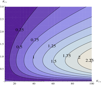
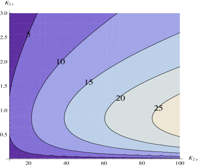
  Figure 1: Contour plots of $R$ (cf. eq (41)) in the flavour swap scenario for $K_{1\tau},K_{1e}\gg 1$, $K_{1\mu}\lesssim 1$, $K_{2e}=K_{2\mu}$. The latter condition implies that the last term in the eq. (86) is negligible. Left panel: $|\varepsilon_{2\mu}|=\varepsilon_{2\mu}^{\rm max}$; right panel: $|\varepsilon_{2\mu}|=0.1\,\varepsilon_{2\mu}^{\rm max}$ (cf. eq. (87)). In both panels $\varepsilon_{2\tau}=\varepsilon_{2\tau}^{\rm max}$ and $\varepsilon_{2\mu}/\varepsilon_{2\tau}>1$.

  We have fixed $K_{1\mu}\lesssim 1$, $K_{1e},K_{1\tau}\gg 1$, so that only the muonic asymmetry survives the lightest RH neutrino wash-out. We have also set $K_{2\mu}/K_{2\gamma}=1/2\gg K_{1\mu}/K_{1\tau}$, so that the last term in the eq. (86) can be neglected. Concerning the $C\!P$ asymmetries, in the left panel we have set $\varepsilon_{2\gamma}=\varepsilon_{2\gamma}^{\rm max}$ and $\varepsilon_{2\tau}=\varepsilon_{2\tau}^{\rm max}$. One can see that in this case the enhancement of the asymmetry becomes relevant when $K_{2\gamma}\gg K_{2\tau}$ but for $K_{2\gamma}\lesssim 100$ (a reasonable maximum value), it cannot be higher than about $R\simeq 2.5$. Notice that, since we choose $\varepsilon_{2\gamma}/\varepsilon_{2\tau}>1$, a reduction is also possible due to a cancelation of the traditional term and of the new term due to flavour coupling. In the right panels we have set $\varepsilon_{2\gamma}=0.1\,\varepsilon_{2\gamma}^{\rm max}$ and this time one can see how $R$ can be as large as one order of magnitude. This shows that for $\varepsilon_{\gamma}\rightarrow 0$ the enhancement can be arbitrarily large.

• Case B: Enhancement from flavour coupling at $N_{1}$ washout

  Another interesting case is when $\kappa(K_{2\gamma})\ll\kappa(K_{2\tau})$ and in addition $P^{0}_{2\delta}/P^{0}_{2\gamma}\ll P^{0}_{1\delta}/P^{0}_{1\tau}$. In this case the first and fourth terms in eq. (86) dominate and we obtain approximately

  $$N_{B-L}^{\rm f}\simeq p_{\delta}-C^{(3)}_{\delta\tau}\,{P^{0}_{1\delta}\over P^{0}_{1\tau}}\,\varepsilon_{2\tau}\,\kappa(K_{2\tau})\,.$$ (89)

We can see that again we have the phantom term avoiding the wash-out at the production and a second term arising from the flavour coupling at the wash-out by $N_{1}$. We note that this term is not even proportional to the flavoured asymmetry $\varepsilon_{2\delta}$ and is just due to the fact that thanks to flavour coupling the wash-out of the large tauonic asymmetry produced at $T\sim T_{L}$ has as a side effect a departure from thermal equilibrium of the processes $N_{1}\leftrightarrow l_{e}+\phi^{\dagger},\bar{l}_{e}+\phi$. This can be understood easily again in terms of the Higgs asymmetry that connects the dynamics in the two flavours. It is quite amusing that thanks to flavour coupling an electron asymmetry is generated even without explicit electronic $C\!P$ violation.

Also for this case B, we have plotted, in the Fig. 2, the $R$ iso-contour lines (cf. eq (41)) in the plane $(K_{2\gamma},K_{2\tau})$.

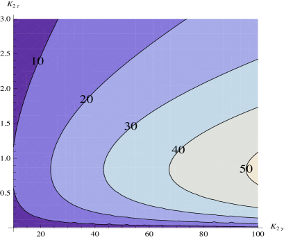
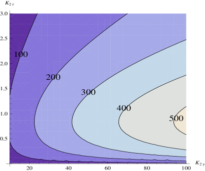
Figure 2: Contour plots of $R$ (cf. eq (41)) in the flavour swap scenario for $K_{1\tau},K_{1\mu}\gg 1$, $K_{1e}\lesssim 1$, $K_{2e}/K_{2\mu}\ll K_{1e}/K_{1\tau}$. The last condition implies that the last term in the eq. (86) dominates. Left panel: $\varepsilon_{2\mu}=\varepsilon_{2\mu}^{\rm max}$; right panel: $\varepsilon_{2\mu}=0.1\,\varepsilon_{2\mu}^{\rm max}$ (cf. eq. (87)). In both panels $\varepsilon_{2\tau}=\varepsilon_{2\tau}^{\rm max}$ and $\varepsilon_{2\mu}/\varepsilon_{2\tau}>1$.

We have set $K_{1e}\lesssim 1$ while $K_{1\mu},K_{1\tau}\gg 1$, so that now only the electron asymmetry survives the lightest RH neutrino wash-out. Moreover this time we have set $K_{2e}/K_{2\gamma}\ll K_{1e}/K_{1\tau}$ so that the last term in the eq. (86) becomes dominant and the case B is realized. For the $C\!P$ asymmetries, as before, in the left panel we fixed $\varepsilon_{2\gamma}=\varepsilon_{2\gamma}^{\rm max}$ while in the right panel $\varepsilon_{2\gamma}=0.1\,\varepsilon_{2\gamma}^{\rm max}$ and in both cases $\varepsilon_{2\tau}=\varepsilon_{2\tau}^{\rm max}$. Now the enhancement of the final asymmetry $R$ is $\gg 1$ in both cases, simply because the traditional term is this time suppressed by $K_{2e}/K_{2\gamma}\ll 1$. This means that after the decoherence of the $\gamma$ lepton quantum states, there is a negligible asymmetry in the electron flavour. However, at the lightest RH neutrino wash-out, an electron asymmetry is generated thanks to flavour coupling.

4.2 Example for Case A within Heavy Sequential Dominance

To find realistic examples where the two cases A and B with strong impact of flavour coupling are realised, we will now consider classes of models with so-called sequential dominance (SD) [32, 33, 34, 35] in the seesaw mechanism. To illustrate case A, we may in particular consider a sub-class called heavy sequential dominance (HSD). To realise case A within HSD, in eq. (86) and eq. (88) we assign flavours $\delta=\mu$ and $\beta=e$.

To understand how heavy sequential dominance works, we begin by writing the RH neutrino Majorana mass matrix $M_{\mathrm{RR}}$ in a diagonal basis as

$$M_{\mathrm{RR}}=\begin{pmatrix}M_{C}&0&0\\ 0&M_{B}&0\\ 0&0&M_{A}\end{pmatrix},$$ (90)

where we have ordered the columns according to $M_{RR}=\mbox{diag}(M_{1},M_{2},M_{3})$ where $M_{1}<M_{2}<M_{3}$. In this basis we write the neutrino (Dirac) Yukawa matrix $\lambda_{\nu}$ in terms of $(1,3)$ column vectors $C_{i},$ $B_{i},$ $A_{i}$ as

$$\lambda_{\nu}=\begin{pmatrix}C&B&A\end{pmatrix},$$ (91)

in the convention where the Yukawa matrix is given in left-right convention. The Dirac neutrino mass matrix is then given by $m_{\mathrm{LR}}^{\nu}=\lambda_{\nu}v_{\mathrm{u}}$. The term for the light neutrino masses in the effective Lagrangian (after electroweak symmetry breaking), resulting from integrating out the massive right handed neutrinos, is

$$\mathcal{L}^{\nu}_{eff}=\frac{(\nu_{i}^{T}A_{i})(A^{T}_{j}\nu_{j})v^{2}}{M_{A}}+\frac{(\nu_{i}^{T}B_{i})(B^{T}_{j}\nu_{j})v^{2}}{M_{B}}+\frac{(\nu_{i}^{T}C_{i})(C^{T}_{j}\nu_{j})v^{2}}{M_{C}}$$ (92)

where $\nu_{i}$ ($i=1,2,3$) are the left-handed neutrino fields. heavy sequential dominance (HSD) then corresponds to the third term being negligible, the second term subdominant and the first term dominant:

$$\frac{A_{i}A_{j}}{M_{A}}\gg\frac{B_{i}B_{j}}{M_{B}}\gg\frac{C_{i}C_{j}}{M_{C}}\,.$$ (93)

In addition, we shall shortly see that small $\theta_{13}$ and almost maximal $\theta_{23}$ require that

$$|A_{1}|\ll|A_{2}|\approx|A_{2}|.$$ (94)

We identify the dominant RH neutrino and Yukawa couplings as $A$, the subdominant ones as $B$, and the almost decoupled (subsubdominant) ones as $C$.

Working in the mass basis of the charged leptons, we obtain for the lepton mixing angles:

$$\tan\theta_{23} \approx \frac{|A_{2}|}{|A_{3}|}\;,$$ (95a)

$$\tan\theta_{12} \approx \frac{|B_{1}|}{c_{23}|B_{2}|\cos\tilde{\phi}_{2}-s_{23}|B_{3}|\sin\tilde{\phi}_{3}}\;,$$ (95b)

$$\theta_{13} \approx e^{i\tilde{\phi}_{4}}\frac{|B_{1}|(A_{2}^{*}B_{2}+A_{3}^{*}B_{3})}{\left[|A_{2}|^{2}+|A_{3}|^{2}\right]^{3/2}}\frac{M_{A}}{M_{B}}+\frac{e^{i\tilde{\phi}_{5}}|A_{1}|}{\sqrt{|A_{2}|^{2}+|A_{3}|^{2}}},$$ (95c)

where the phases do not need to concern us.

The neutrino masses are:

$$m_{3} \approx \frac{(|A_{2}|^{2}+|A_{3}|^{2})v^{2}}{M_{A}}\;,$$ (96a)

$$m_{2} \approx \frac{|B_{1}|^{2}v^{2}}{s^{2}_{12}M_{B}}\;,$$ (96b)

$$m_{1} \approx {\cal O}(|C|^{2}v^{2}/M_{C})\;.$$ (96c)

Tri-bimaximal mixing corresponds to:

$$|A_{1}| = 0,$$ (97)

$$\text{\ }|A_{2}| = |A_{3}|,$$ (98)

$$|B_{1}| = |B_{2}|=|B_{3}|,$$ (99)

$$A^{\dagger}B = 0.$$ (100)

This is called constrained sequential dominance (CSD).

For $N_{2}$ leptogenesis, the flavour specific decay asymmetries are $\varepsilon_{2\alpha}$ where the leading contribution comes from the heavier RH neutrino of mass $M_{A}=M_{3}$ in the loop which may be approximated via eq. (11) as:

$$\varepsilon_{2\alpha}\approx-\frac{3}{16\pi v^{2}}\frac{M_{2}}{M_{3}}\frac{1}{B^{\dagger}B}\mathrm{Im}\left[B_{\alpha}^{*}(B^{\dagger}A)A_{\alpha}\right].$$ (101)

Clearly the asymmetry vanishes in the case of CSD due to eq. (100) and so in the following we shall consider examples which violate CSD. The mixing angles are given by the following estimates:

$$\tan\theta_{23}\sim\frac{A_{2}}{A_{3}}\sim 1,\ \ \tan\theta_{12}\sim\frac{\sqrt{2}B_{1}}{B_{2}+B_{3}}\sim\frac{1}{\sqrt{2}},\ \ \theta_{13}\sim\frac{A_{1}}{\sqrt{2}A_{2}}\sim\frac{r}{\sqrt{2}}.$$ (102)

Suppose we parametrize the Yukawa couplings consistent with these mixing angles as:

$$A_{2}=A_{3},\ \ A_{1}=r\,A_{2},\ \ B_{3}=q\,B_{2},\ \ B_{1}=\frac{1}{2}(1+q)\,B_{2}\ \$$ (103)

where $r<1$ is related to $\theta_{13}$ and $\theta_{12}$ via eq. (102), then we find,

$$\varepsilon_{2\mu}\approx-\frac{3}{16\pi v^{2}}\,M_{2}m_{3},\ \ \varepsilon_{2\tau}\approx q\,\varepsilon_{2\mu},\ \ \varepsilon_{2e}\approx\frac{r}{2}\,\varepsilon_{2\mu}.$$ (104)

The flavoured effective neutrino masses $\widetilde{m}_{2\alpha}$, $\widetilde{m}_{1\alpha}$ are given by:

$$\widetilde{m}_{2\alpha}=\frac{|B_{\alpha}|^{2}v^{2}}{M_{B}}\sim m_{2}\,,\,\,\widetilde{m}_{1\alpha}=\frac{|C_{\alpha}|^{2}v^{2}}{M_{C}}\sim m_{1}\,.$$ (105)

Neutrino oscillation experiments tell us that $r<1$ is small (here we shall assume $r\sim 0.2$ as a specific example consistent with current experimental results) and we find

$$K_{2\mu}={\widetilde{m}_{2\mu}\over m_{\star}}\sim{m_{2}\over m_{\star}}\sim 10,\,\,K_{2e}\sim\frac{(1+q)^{2}}{4}\,K_{2\mu},\,\,K_{2\tau}\sim q^{2}\,K_{2\mu},$$ (106)

which allows strong washout for $K_{2\gamma}$ ($\gamma=\mu+e$) with weak washout for $K_{2\tau}$. By assuming that $C_{1},C_{2}\ll C_{3}$ we have,

$$K_{1\tau}={\widetilde{m}_{1\tau}\over m_{\star}}\sim 10\,\frac{m_{1}}{m_{2}},\,\,K_{1e},\,K_{1\mu}\ll K_{1\tau}$$ (107)

which allows for strong washout for $K_{1\tau}$ (at least if $m_{1}\sim m_{2}$) with weak washouts for $K_{1e},K_{1\mu}$.

Thus, without flavour coupling and phantom terms, we would have strong (exponential) $N_{1}$ washout for $K_{1\tau}\sim 10$, with negligible $N_{1}$ washout for $K_{1e},K_{1\mu}<1$. Since $\varepsilon_{2e}\approx\frac{r}{2}\varepsilon_{2\mu}\sim 0.1\varepsilon_{2\mu}$ we may neglect $\varepsilon_{2e}$ and then we find that the term proportional to $\varepsilon_{2\gamma}\,\kappa(K_{2\gamma})$ is strongly washed out since $K_{2\gamma}\sim 10$. Therefore, without flavour coupling and phantom effects, $N_{B-L}^{\rm f}$ would tend to be small in this scenario.

While, allowing for the effects of flavour redistribution and including the phantom term, we find (cf. eq. (88)),

$$N_{B-L}^{\rm f}\sim p_{\mu}+{K_{2\mu}\over K_{2\gamma}}\,\varepsilon_{2\gamma}\,\kappa(K_{2\gamma})-{K_{2\mu}\over K_{2\gamma}}C^{(2)}_{\gamma\tau}\,\varepsilon_{2\tau}\,\kappa(K_{2\tau})\,.$$ (108)

Since $K_{2\mu}/K_{2\gamma}\simeq 4/(5+2\,q)$ and $p_{\mu}\simeq[(1+2q)/(5+2q)]\varepsilon_{2\mu}\,N_{N_{2}}^{\rm in}$, then we have

$$N_{B-L}^{\rm f}\sim{1+2q\over 5+2q}\,\varepsilon_{2\mu}\,N_{N_{2}}^{\rm in}+{4\over 4+(1+q)^{2}}\,\left[\varepsilon_{2\gamma}\,\kappa(K_{2\gamma})-\,C^{(2)}_{\gamma\tau}\varepsilon_{2\tau}\,\kappa(K_{2\tau})\right]\,,$$ (109)

where $K_{2\tau}\sim q^{2}\,K_{2\mu}\sim 10\,q^{2}$ leads to only weak wash out with $\varepsilon_{2\mu}\sim-\frac{3}{16\pi v^{2}}M_{2}\,m_{3}$ being large. Notice that there is a partial cancelation of the two terms but this is just depending on the particular choice of values for $r$ and $q$ and on $N_{N_{2}}^{\rm in}$. This is an example, consistent with neutrino data, where $N_{B-L}^{\rm f}$ would be very small without flavour coupling and phantom term, but will be quite large including the two effects that both produce a large contribution. If we indeed, for definiteness, assume $N_{N_{2}}^{\rm in}=0$ and $q\sim 0.5$ such that $K_{2\tau}\sim 1$ corresponding to $\kappa(K_{2\tau})\simeq 0.3$, then we find for $R$ (cf. eq (41))

$$R\simeq\left|1-C^{(2)}_{\gamma\tau}\,{\kappa(K_{2\tau})\over\kappa(K_{2\gamma})}\,{\varepsilon_{2\,\tau}\over\varepsilon_{2\gamma}}\right|\,.$$ (110)

In Fig. (3) we plotted $R$ as a function of $q=\varepsilon_{2\tau}/\varepsilon_{2\mu}$. One can see that this example realizes a specific case of the general situation shown in the left panel of Fig. 1. In particular, one can see that there can be a relevant suppression for positive $q$ and up to a $50\%$ enhancement for negative $q$.

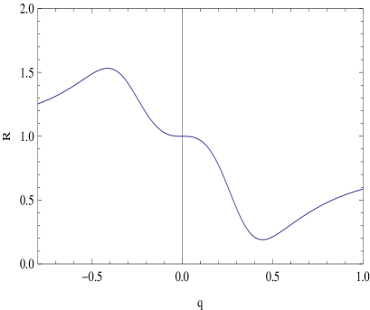
Figure 3: Plot of $R$ as a function of $q$ as from the eq. (110).

On the other hand, in case of initial thermal abundance, one can easily verify that the presence of the phantom term can yield an enhancement up to three orders of magnitude.

4.3 Example for Case B within Light Sequential Dominance

To give an example for case B (i.e. an example where $K_{1e}\ll K_{1\mu},K_{1\tau}$ while $\varepsilon_{2\tau}\gg\varepsilon_{2\mu},\varepsilon_{2e}$ and $K_{2e}\ll K_{2\gamma}$), we may consider another class of sequential dominance, namely light sequential dominance (LSD). Now, in eq. (86) and eq. (89) we have to replace $\delta=e$ and $\beta=\mu$.

In the example of LSD we will consider, using the same notation for the dominant, subdominant and subsubdominant RH neutrinos and corresponding couplings, we have:

$$M_{\mathrm{RR}}=\begin{pmatrix}M_{A}&0&0\\ 0&M_{C}&0\\ 0&0&M_{B}\end{pmatrix}.$$ (111)

The lightest RH neutrino with mass $M_{A}$ dominates the seesaw mechanism. We have again ordered the columns according to $M_{RR}=\mbox{diag}(M_{1},M_{2},M_{3})$ where $M_{1}<M_{2}<M_{3}$. For the neutrino (Dirac) Yukawa matrix we use the notation

$$\lambda_{\nu}=\begin{pmatrix}A_{1}&C_{1}&B_{1}\\ A_{2}&C_{2}&B_{2}\\ A_{3}&C_{3}&B_{3}\end{pmatrix},.$$ (112)

More specifically, let us now consider, within LSD, a variant of CSD called partially constrained sequential dominance (PCSD) [36] where $|A_{2}|=|A_{3}|=a$ and $|B_{1}|=|B_{2}|=|B_{3}|=b$, but $A_{1}\not=0$. In addition, we may assume $C=(C_{1},C_{2},C_{3})$ with $C_{1}=0$ and $C_{2}/C_{3}=\zeta\ll 1$ as a specific example. Under these conditions, and using $A_{1}=rA_{2}=\sqrt{2}\theta_{13}A_{2}$ defined in the previous section, we can write the neutrino Yukawa matrix as

$$\lambda_{\nu}=\begin{pmatrix}\sqrt{2}\theta_{13}a&0&b\\ a&\zeta c&b\\ -a&c&b\end{pmatrix}.$$ (113)

The flavoured effective neutrino masses $\widetilde{m}_{2\alpha}$, $\widetilde{m}_{1\alpha}$ in this specific LSD scenario are given by:

$$\widetilde{m}_{2\alpha}=\frac{|C_{\alpha}|^{2}v^{2}}{M_{C}}\sim m_{2},\ \ \widetilde{m}_{1\alpha}=\frac{|A_{\alpha}|^{2}v^{2}}{M_{A}}\;.$$ (114)

For $\widetilde{m}_{1e}$, $\widetilde{m}_{1\mu}$ and $\widetilde{m}_{1\tau}$ we obtain explicitly

$$\widetilde{m}_{1e}=\frac{|\sqrt{2}\,\theta_{13}\,a|^{2}v^{2}}{M_{1}}=m_{3}\,\theta_{13}^{2},\ \ \widetilde{m}_{1\mu}=\widetilde{m}_{1\tau}=\frac{|a|^{2}v^{2}}{M_{1}}=\frac{m_{3}}{2}\;.$$ (115)

The parameters $K_{i\alpha}$ are related to the $\widetilde{m}_{i\alpha}$’s simply by $K_{i\alpha}=\widetilde{m}_{i\alpha}/m^{*}$. Since we know from neutrino oscillation experiments that the leptonic mixing angle $\theta_{13}$ is small (at least $<10^{\circ}$) we have that $K_{1e}\ll K_{1\mu}=K_{1\tau}$, i.e.

$$K_{1\mu}=K_{1\tau}\sim{m_{3}\over m^{*}}\sim 50$$ (116)

and

$$\frac{K_{1e}}{K_{1\mu}}=\frac{K_{1e}}{K_{1\tau}}=(\sqrt{2}\theta_{13})^{2}\;.$$ (117)

Consequently, the asymmetries in the $\tau$ and in the $\mu$ flavours will be almost completely washed out by the $N_{1}$ washout related to $K_{1\tau}$ and $K_{1\mu}$. In the $e$-flavour we have weak $N_{1}$-washout.

Furthermore, using $\frac{|C_{\alpha}|^{2}v^{2}}{M_{C}}\sim m_{1}$, we obtain at the $N_{2}$ decay stage

$$K_{2\tau}\sim{m_{1}\over m^{*}},\ \ K_{2\mu}\sim\zeta\,{m_{1}\over m^{*}}\ll K_{2\tau},\ \mbox{and}\,\,K_{2e}=0\>,$$ (118)

which implies

$$K_{2\gamma}=K_{2\mu}+K_{2e}\ll K_{2\tau}\>.$$ (119)

The $N_{2}$ decay asymmetries, ignoring the contribution with $N_{1}$ in the loop which is very small for the considered case that $N_{1}\ll N_{2}$, are given via eq. (11) by

$$\varepsilon_{2\alpha}\approx-\frac{3}{16\pi v^{2}}\frac{M_{2}}{M_{3}}\frac{1}{B^{\dagger}B}\mathrm{Im}\left[B_{\alpha}^{*}(B^{\dagger}C)C_{\alpha}\right].$$ (120)

Using $B$ and $C$ as specified above eq. (113) and $m_{1}\sim\frac{|C_{\alpha}|^{2}v^{2}}{M_{C}}$, we obtain for the decay asymmetries $\varepsilon_{2\alpha}$:

$$\varepsilon_{2\tau}\sim-\frac{3}{16\pi v^{2}}\,M_{2}\,m_{2},\ \ \varepsilon_{2\mu}=\zeta\varepsilon_{2\tau}\ll\varepsilon_{2\tau},\ \ \varepsilon_{2e}=0\;.$$ (121)

Considering eq. (86) and noting that $K_{2e}=0$ together with $\varepsilon_{2e}=0$ implies $p_{\delta}=0$ we see that all terms apart from the one proportional to $C^{(3)}_{e\tau}$ are strongly suppressed provided that $\zeta$ is sufficiently tiny ($\zeta\ll r$). In other words, the considered LSD scenario provides an example for case B, a final asymmetry dominated by flavour coupling effects at the $N_{1}$ washout stage, as in eq. (89). Explicitly, we obtain for the final asymmetry

$$N_{B-L}^{\rm f}\sim-C^{(3)}_{e\tau}\,{K_{1e}\over K_{1\tau}}\,\varepsilon_{2\tau}\,\kappa(K_{2\tau})\sim\frac{3C^{(3)}_{e\tau}}{16\pi}\frac{M_{2}\,m_{2}}{v^{2}}(\sqrt{2}\theta_{13})^{2}\kappa\left(\frac{m_{1}}{m^{*}}\right).$$ (122)

Here one can see that

$$R\simeq 1+0.01\,\zeta^{-1}\,\left({\theta_{13}\over 10^{\circ}}\right)^{2}\,{\kappa(m_{1}/m_{\star})\over 0.3}\,.$$ (123)

This result shows quite interestingly that, if $\theta_{13}\neq 0$ and $m_{1}\gtrsim m_{\star}$, one can obtain a huge enhancement for $\xi\rightarrow 0$, indicating that, accounting for flavour coupling, one can have an asymmetry in a situation where one would otherwise obtain basically a zero asymmetry. This happens because part of the tauon asymmetry, thanks to flavour coupling at the lightest RH neutrino wash-out, escapes the wash out from the lightest RH neutrinos.

5 Conclusions

We have discussed various new flavour dependent effects in the $N_{2}$-dominated scenario of leptogenesis and have shown that these effects are important in obtaining a reliable expression for the final asymmetry. In particular we have emphasized the importance of the off-diagonal entries of the flavour coupling matrix that connects the total flavour asymmetries, distributed in different particle species, to the lepton and Higgs doublet asymmetries. We have derived analytical formulae for the final asymmetry including the flavour coupling at the $N_{2}$-decay stage, where effectively two flavours are active, as well as at the stage of washout by the lightest RH neutrino $N_{1}$ where all three flavours are distinguished. The interplay between the production stage and the wash-out stage can then result in a significant enhancement of the final asymmetry.

We have also described a completely new effect, “phantom leptogenesis”, where the lightest RH neutrino wash-out is actually able to create a $B-L$ asymmetry rather than destroying it as usually believed. This is possible because the individual wash-out on each flavoured asymmetry can erase cancelations among the electron and muon phantom terms and therefore lead to a net increase of the total $B-L$ asymmetry. In this way the wash-out at the production is basically fully circumvented for part of the produced electron and muon asymmetries. We also noticed however that the phantom terms also strongly depend on the specific initial conditions since they are proportional to the initial $N_{2}$-abundance and therefore, in particular, they vanish for initial zero $N_{2}$-abundance.

The changes induced by these new effects are encoded in the general “master formula” eq. (77) for the final asymmetry that we derived from the Boltzmann equations without approximations. Based on this equation we have identified a sufficiently generic scenario, the “flavour swap scenario”, where we proved that a strong enhancement of the final asymmetry due to flavour coupling and phantom terms is clearly possible. The conditions for the flavour swap scenario correspond to have a one flavour dominated asymmetry at the production, in the two flavour regime, and a wash-out from the lightest RH neutrinos swapping the dominance from one flavour to the other. Flavour coupling can strongly modify the flavour asymmetry that is subdominant at the production inducing two new contributions, one generated at the production and one at the lightest RH neutrino wash-out. Then, in the flavour swap scenario, this translates into a strong modification of the final asymmetry after the lightest RH neutrino wash-out. It is quite interesting that, because of flavour coupling, an asymmetry is actually generated by the wash-out terms that therefore in this case act more like wash-in terms, transmitting a departure from thermal equilibrium from one flavour to the other. In the figures we have showed how, once the flavour swap scenario, is realized, relevant modifications of the final asymmetry are generically induced by flavour coupling. Depending on the values of the involved parameters, these range from ${\cal O}(1)$ factor changes (either a reduction or an enhancement) to an orders of magnitude enhancement.

We have illustrated these effects for two models which describe realistic neutrino masses and mixing based on sequential dominance.

In conclusion, the off-diagonal flavour couplings as well as phantom terms can have a significant impact on the baryon asymmetry produced by $N_{2}$-dominated leptogenesis and thus have to be included in a reliable analysis. We have derived exact analytic (and also compact approximate) results that allow this to be achieved. The results in this paper open up new possibilities for successful $N_{2}$-dominated leptogenesis to explain the baryon asymmetry of the universe.

Acknowledgments

S.A.  acknowledges partial support from the DFG cluster of excellence “Origin and Structure of the Universe”. P.D.B. acknowledges financial support from the NExT Institute and SEPnet. S.F.K. was partially supported by the following grants: STFC Rolling Grant ST/G000557/1 and a Royal Society Leverhulme Trust Senior Research Fellowship. P.D.B wishes to thank Antonio Riotto and Steve Blanchet for useful discussions.

Appendix A

In this Appendix we recast eq. (77) in a more extensive way in order to illustrate a generic feature of it. Each final $\alpha$ asymmetry is now the sum of three contributions,

$$N^{\rm f}_{\Delta_{\alpha}} = V^{-1}_{\alpha e^{\prime\prime}}\,\left[\sum_{\beta}\,V_{e^{\prime\prime}\beta}\,N_{\Delta_{\beta}}^{T\sim T_{L}}\right]\,e^{-{3\pi\over 8}\,K_{1e^{\prime\prime}}}$$

$$+ V^{-1}_{\alpha\mu^{\prime\prime}}\,\left[\sum_{\beta}\,V_{\mu^{\prime\prime}\beta}\,N_{\Delta_{\beta}}^{T\sim T_{L}}\right]\,e^{-{3\pi\over 8}\,K_{1\mu^{\prime\prime}}}$$

$$+ V^{-1}_{\alpha\tau^{\prime\prime}}\,\left[\sum_{\beta}\,V_{\tau^{\prime\prime}\beta}\,N_{\Delta_{\beta}}^{T\sim T_{L}}\right]\,e^{-{3\pi\over 8}\,K_{1\tau^{\prime\prime}}}\,.$$

In the approximation $K_{1\epsilon^{\prime\prime}}\simeq K_{1e}$, $K_{1\mu^{\prime\prime}}\simeq K_{1\mu}$, $K_{1\tau^{\prime\prime}}\simeq K_{1\tau}$, it becomes

$$N^{\rm f}_{\Delta_{\alpha}} \simeq V^{-1}_{\alpha e^{\prime\prime}}\,\left[\sum_{\beta}\,V_{e^{\prime\prime}\beta}\,N_{\Delta_{\beta}}^{T\sim T_{L}}\right]\,e^{-{3\pi\over 8}\,K_{1e}}$$

$$+ V^{-1}_{\alpha\mu^{\prime\prime}}\,\left[\sum_{\beta}\,V_{\mu^{\prime\prime}\beta}\,N_{\Delta_{\beta}}^{T\sim T_{L}}\right]\,e^{-{3\pi\over 8}\,K_{1\mu}}$$

$$+ V^{-1}_{\alpha\tau^{\prime\prime}}\,\left[\sum_{\beta}\,V_{\tau^{\prime\prime}\beta}\,N_{\Delta_{\beta}}^{T\sim T_{L}}\right]\,e^{-{3\pi\over 8}\,K_{1\tau}}\,.$$

This expression shows how now each $\alpha$ asymmetry is not simply given by one term containing a $N_{1}$ wash-out exponential suppression term described by $e^{-3\pi\,K_{1\alpha}/8}$ but it also contains terms that are washed out by exponentials $e^{-3\pi\,K_{1\delta\neq\alpha}/8}$. In this way, even though $K_{1\alpha}\gg 1$, there can still be unsuppressed contributions to $N^{\rm f}_{\Delta_{\alpha}}$ from terms with $K_{1\delta\neq\alpha}\ll 1$. Even though these terms are weighted by factors $V^{-1}_{\alpha\delta}$ containing off-diagonal terms of the $C^{(3)}$ matrix, they can be dominant in some cases and therefore, in general, they have to be accounted for.

We can also recast this last equation in even a more explicit form unpacking the second sum as well,

$$N^{\rm f}_{\Delta_{\alpha}} \simeq V^{-1}_{\alpha e^{\prime\prime}}\,\left[V_{e^{\prime\prime}e}\,N_{\Delta_{e}}^{T\sim T_{L}}+V_{e^{\prime\prime}\mu}\,N_{\Delta_{\mu}}^{T\sim T_{L}}+V_{e^{\prime\prime}\tau}\,N_{\Delta_{\tau}}^{T\sim T_{L}}\right]\,e^{-{3\pi\over 8}\,K_{1e}}$$

$$+ V^{-1}_{\alpha\mu^{\prime\prime}}\,\left[V_{\mu^{\prime\prime}e}\,N_{\Delta_{e}}^{T\sim T_{L}}+V_{\mu^{\prime\prime}\mu}\,N_{\Delta_{\mu}}^{T\sim T_{L}}+V_{\mu^{\prime\prime}\tau}\,N_{\Delta_{\tau}}^{T\sim T_{L}}\right]\,e^{-{3\pi\over 8}\,K_{1\mu}}$$

$$+ V^{-1}_{\alpha\tau^{\prime\prime}}\,\left[V_{\tau^{\prime\prime}e}\,N_{\Delta_{e}}^{T\sim T_{L}}+V_{\tau^{\prime\prime}\mu}\,N_{\Delta_{\mu}}^{T\sim T_{L}}+V_{\tau^{\prime\prime}\tau}\,N_{\Delta_{\tau}}^{T\sim T_{L}}\right]\,e^{-{3\pi\over 8}\,K_{1\tau}}\,.$$

Appendix B

In this Appendix we show how the results on phantom leptogenesis can be also derived within a density matrix formalism. We report results from [37], where a more general and detailed discussion can be found. Let us recall that we treat the three stages of $N_{2}$ production at $T\sim T_{L}$, decoherence at $T^{\star}\sim 10^{9}\,$GeV and the lightest RH neutrino wash-out at $T\sim M_{1}\ll 10^{9}\,$GeV, as completely separate from each other. This allows a simplification of the discussion. In order to simplify the notation, in this Appendix we also assume that the quantum states $|\ell_{2}\rangle$ and $|\bar{\ell}^{\prime}_{2}\rangle$ do not have any tauon component, i.e. $P_{2\tau}=\bar{P}_{2\tau}=P^{0}_{2\tau}=0$ and consequently $P_{2\gamma}=\bar{P}_{2\gamma}=P^{0}_{2\gamma}=1$.

The flavour composition of the lepton and anti-lepton quantum states can then be written as $(\alpha=e,\mu)$

$$|{\ell}_{2}\rangle = {\cal C}_{2e}\,|{\ell}_{e}\rangle+{\cal C}_{2\mu}\,|{\ell}_{\mu}\rangle\,,\;\;\;{\cal C}_{2\alpha}\equiv\langle{\ell}_{\alpha}|\ell_{2}\rangle\,,$$ (B.1)

$$|\bar{\ell}^{\prime}_{2}\rangle = \bar{{\cal C}}_{2e}\,|\bar{{\ell}}_{e}\rangle+\bar{{\cal C}}_{2\mu}\,|\bar{{\ell}}_{\mu}\rangle\,,\;\;\;\bar{{\cal C}}_{2\alpha}\equiv\langle\bar{{\ell}}_{\alpha}|\bar{\ell}^{\prime}_{2}\rangle\,,$$ (B.2)

where $P_{2\alpha}=|{\cal C}_{2\alpha}|^{2}$ and $\bar{P}_{2\alpha}=|\bar{\cal C}_{2\alpha}|^{2}$. At the $N_{2}$-production, at $T\sim T_{L}\gg 10^{9}\,{\rm GeV}$, muon charged lepton interactions are ineffective and therefore the $|\ell_{2}\rangle$ and $|\bar{\ell}^{\prime}_{2}\rangle$ quantum states evolve coherently. In this case, in the two different bases $\ell_{2}-\ell_{2}^{\bot}$ and $\bar{\ell}^{\prime}_{2}-\bar{\ell}_{2}^{{}^{\prime}\bot}$, the lepton and anti-lepton density matrices are respectively simply given by

$$\rho^{\ell_{2}}_{ij}\equiv\langle i|{\ell}_{2}\rangle\langle{\ell}_{2}|j\rangle={\rm diag}(1,0)\hskip 14.22636pt\mbox{\rm and}\hskip 14.22636pt\rho^{\bar{\ell}^{\prime}_{2}}_{\bar{i}\bar{j}}\equiv\langle\bar{i}|\bar{\ell}^{\prime}_{2}\rangle\langle\bar{\ell}^{\prime}_{2}|\bar{j}\rangle={\rm diag}(1,0)\,,$$ (B.3)

where $|i\rangle,|j\rangle=|{\ell_{2}}\rangle,|{\ell^{\bot}_{2}}\rangle$ and $|\bar{i}\rangle,|\bar{j}\rangle=|{\bar{\ell}^{\prime}_{2}}\rangle,|{\bar{\ell}^{{}^{\prime}\bot}_{2}}\rangle$. It is crucial to notice that, because of the different flavour composition of $|\ell_{2}\rangle$ and $|\bar{\ell}^{\prime}_{2}\rangle$, the two bases are not $C\!P$ conjugated of each other. If we introduce the lepton number and anti-lepton number density matrices, $N^{\ell_{2}}_{ij}\equiv N_{\ell_{2}}\,\rho^{\ell_{2}}_{ij}$ and $N^{\bar{\ell}^{\prime}_{2}}_{\bar{i}\bar{j}}\equiv N_{\ell_{2}}\,\rho^{\bar{\ell}^{\prime}_{2}}_{\bar{i}\bar{j}}$ respectively, their evolution at $T\sim T_{L}$ is given by

$${dN^{\ell_{2}}_{ij}\over dz_{2}}=\left({\Gamma_{2}\over H\,z_{2}}\,N_{N_{2}}-{\Gamma_{2}^{ID}\over H\,z_{2}}\,N_{\ell_{2}}\right)\,\rho^{\ell_{2}}_{ij}\,,\;\;\hskip 14.22636pt{dN^{\bar{\ell}^{\prime}_{2}}_{\bar{i}\bar{j}}\over dz_{2}}=\left({\bar{\Gamma}_{2}\over H\,z_{2}}\,N_{N_{2}}-{\bar{\Gamma}_{2}^{ID}\over H\,z_{2}}\,N_{\bar{\ell}_{2}}\right)\,\rho^{\bar{\ell}^{\prime}_{2}}_{\bar{i}\bar{j}}\,.$$ (B.4)

In order to obtain an equation for the total $B-L$ asymmetry $N_{B-L}$ at $T\simeq T_{L}$, we have first to write these two equations in the same flavour basis for leptons and anti-leptons, that for our objectives can be conveniently chosen to be $e-\mu$ and $\bar{e}-\bar{\mu}$ respectively, and then subtract them. Introducing the rotation operators $R$ and $\hat{R}$, such that $|{\ell}_{2}\rangle=\hat{R}\,|e\rangle$, $|{\ell}^{\bot}_{2}\rangle=\hat{R}\,|\mu\rangle$ and $|\bar{\ell}^{\prime}_{2}\rangle=\hat{\bar{R}}\,|\bar{e}\rangle$, $|\bar{\ell}^{{}^{\prime}\bot}_{2}\rangle=\hat{\bar{R}}\,|\bar{\mu}\rangle$, the corresponding rotations matrices $R_{i\alpha}$ and $\bar{R}_{i\alpha}$ are

$$R_{i\alpha}=\left(\begin{array}[]{cc}{\cal C}_{2e}&-{\cal C}_{2\mu}\\ {\cal C}_{2\mu}&{\cal C}_{2e}\end{array}\right)\hskip 28.45274pt\mbox{\rm and}\hskip 28.45274pt\bar{R}_{\bar{i}\bar{\alpha}}=\left(\begin{array}[]{cc}\bar{\cal C}_{2e}&-\bar{\cal C}_{2\mu}\\ \bar{\cal C}_{2\mu}&\bar{\cal C}_{2e}\end{array}\right)$$ (B.5)

for leptons and anti-leptons respectively. In the lepton flavour basis one can finally write the equation for the $B-L$ asymmetry density matrix

$${dN^{B-L}_{\alpha\beta}\over dz_{2}}=\bar{R}^{\dagger}_{\bar{\alpha}\bar{i}}\,{dN^{\bar{\ell}_{2}}_{\bar{i}\bar{j}}\over dz_{2}}\,\bar{R}_{\bar{j}\bar{\beta}}-R^{\dagger}_{\alpha i}\,{dN^{\ell_{2}}_{ij}\over dz_{2}}\,R_{j\beta}\,.$$ (B.6)

For the relevant diagonal components one finds

$${dN^{B-L}_{ee}\over dz_{2}} = \varepsilon_{2e}\,D_{2}\,(N_{N_{2}}-N_{N_{2}}^{\rm eq})-P_{2e}^{0}\,W_{2}\,N_{B-L}\,,$$ (B.7)

$${dN^{B-L}_{\mu\mu}\over dz_{2}} = \varepsilon_{2\mu}\,D_{2}\,(N_{N_{2}}-N_{N_{2}}^{\rm eq})-P_{2\mu}^{0}\,W_{2}\,N_{B-L}\,.$$ (B.8)

Summing these two equations, one finds the usual equation for the total $B-L$ asymmetry $N_{B-L}={\rm Tr}[N^{B-L}_{\alpha\beta}]$,

$${dN_{B-L}\over dz_{2}}=\varepsilon_{2}\,D_{2}\,(N_{N_{2}}-N_{N_{2}}^{\rm eq})-W_{2}\,N_{B-L}\,,$$ (B.9)

that is washed-out at the production. On the other hand, from the two eqs. (B.7) and (B.8), one also obtains

$${1\over P^{0}_{2e}}\,{dN^{B-L}_{ee}\over dz_{2}}-{1\over P^{0}_{2\mu}}\,{dN^{B-L}_{\mu\mu}\over dz_{2}}=-{\Delta P^{0}_{2e}\over 2}\,\left({1\over P^{0}_{2e}}+{1\over P^{0}_{2\mu}}\right)\,D_{2}\,(N_{N_{2}}-N_{N_{2}}^{\rm eq})\,$$ (B.10)

and from this finally

$$N^{B-L}_{ee}(T\simeq T_{L})=P^{0}_{2e}\,N_{B-L}^{T\simeq T_{L}}-{\Delta P_{2e}\over 2}\,N_{N_{2}}^{\rm in}\,,\,\,N^{B-L}_{\mu\mu}(T\simeq T_{L})\simeq P^{0}_{2\mu}\,N_{B-L}^{T\simeq T_{L}}+{\Delta P_{2e}\over 2}\,N_{N_{2}}^{\rm in}\,.$$ (B.11)

If we assume that $N_{B-L}$ is so strongly washed-out that the terms $\propto N_{B-L}^{T\simeq T_{L}}$ can be neglected, one has $N^{B-L}_{ee}(T\simeq T_{L})\simeq-(\Delta P_{2e}/2)\,N_{N_{2}}^{\rm in}\simeq-N^{B-L}_{\mu\mu}(T\simeq T_{L})$. At this stage the electron and muon asymmetries are not measured and cannot have any physical consequence.

However afterwards, at $T\sim T^{\star}=10^{9}\,$GeV, the coherence of the lepton quantum states is broken by the muon lepton interactions and the electron and muon asymmetries are measured by the thermal bath. One can show that the charged lepton interactions give rise to additional terms in the eq. (B.6) [18] that have the effect to damp the off-diagonal terms in $N^{B-L}_{\alpha\beta}$. The electron and muon asymmetries are reprocessed by sphaleron processes and they correspond to $\Delta_{e}$ and $\Delta_{\mu}$ asymmetries, $N_{\Delta_{e}}^{T_{L}}=N^{B-L}_{ee}$, $N_{\Delta_{\mu}}^{T_{L}}=N^{B-L}_{\mu\mu}$ that are now measured by the thermal bath. Nevertheless, at $T\sim T^{\star}$ and down to $T\gtrsim M_{1}$, they still do not give any contribution to the baryon asymmetry (in this sense they are phantom) since they still cancel with each other. However, after the $N_{1}$-wash out at $T\lesssim M_{1}$, one finally has

$$N_{B-L}^{\rm f}\simeq-{\Delta P_{2e}\over 2}\,N_{N_{2}}^{\rm in}\,e^{-{3\pi\over 8}\,K_{1e}}+{\Delta P_{2e}\over 2}\,N_{N_{2}}^{\rm in}\,e^{-{3\pi\over 8}\,K_{1\mu}}$$ (B.12)

that is nothing else than the eq. (67) specialized to the case $P^{0}_{2\gamma}=\varepsilon_{2\tau}=\kappa(K_{2\gamma})=0$ (it is just a simple exercise to include a tauon component re-obtaining exactly the eq. (67)). Finally if, for example, one assumes $K_{1e}\lesssim 1$ and $K_{1\mu}\gg 1$ , then $N_{B-L}^{\rm f}\simeq N_{\Delta_{e}}^{\rm f}\simeq-\Delta P_{2e}\,N_{N_{2}}^{\rm in}$: the unwashed phantom term gets finally imprinted into the final asymmetry. It is worth to notice again that phantom leptogenesis has the attractive feature to provide a way to circumvent completely the wash-out at the production but, on the other hand, it also has the drawback that the final asymmetry strongly depends on the initial $N_{2}$ abundance. Therefore, we have shown how phantom leptogenesis can be also described within a density matrix formalism reproducing the results obtained in the main text in the Boltzmann formalism. The actual practical advantage of the density matrix formalism is that it allows to extend the description beyond the limit where the three stages are fully separated, in a way that the final asymmetry can be calculated for a generic choice of the RH neutrino masses [37]. Notice that these results extend those obtained in [18, 38] within $N_{1}$ leptogenesis, to the case where more heavy neutrino flavours contribute to the final asymmetry. In [18, 38] the lepton and anti-lepton density matrices were assumed to be diagonalizable in bases that are $C\!P$ conjugated of each other and in this case phantom terms cannot be derived. However, within $N_{1}$ leptogenesis, this does not affect the final asymmetry since phantom terms cancel anyway.

References

- [1] M. Fukugita, T. Yanagida, Phys. Lett. B 174 (1986) 45.
- [2] P. Minkowski, Phys. Lett. B 67 (1977) 421; T. Yanagida, in Workshop on Unified Theories, KEK report 79-18 (1979) p. 95; M. Gell-Mann, P. Ramond, R. Slansky, in Supergravity (North Holland, Amsterdam, 1979) eds. P. van Nieuwenhuizen, D. Freedman, p. 315; S.L. Glashow, in 1979 Cargese Summer Institute on Quarks and Leptons (Plenum Press, New York, 1980) p. 687; R. Barbieri, D. V. Nanopoulos, G. Morchio and F. Strocchi, Phys. Lett. B 90 (1980) 91; R. N. Mohapatra and G. Senjanovic, Phys. Rev. Lett. 44 (1980) 912.
- [3] M. C. Gonzalez-Garcia and M. Maltoni, Phys. Rept. 460 (2008) 1.
- [4] E. Komatsu et al. [WMAP Collaboration], Astrophys. J. Suppl. 180 (2009) 330 [arXiv:0803.0547 [astro-ph]].
- [5] S. Davidson and A. Ibarra, Phys. Lett. B 535 (2002) 25 [arXiv:hep-ph/0202239].
- [6] W. Buchmuller, P. Di Bari and M. Plumacher, Nucl. Phys. B 643 (2002) 367.
- [7] S. Blanchet and P. Di Bari, JCAP 0703 (2007) 018 [arXiv:hep-ph/0607330].
- [8] W. Buchmuller, P. Di Bari and M. Plumacher, Annals Phys. 315 (2005) 305 [arXiv:hep-ph/0401240].
- [9] S. Antusch, S. F. King and A. Riotto, JCAP 0611 (2006) 011 [arXiv:hep-ph/0609038].
- [10] S. Antusch and A. M. Teixeira, JCAP 0702 (2007) 024 [arXiv:hep-ph/0611232].
- [11] G. C. Branco, R. Gonzalez Felipe, F. R. Joaquim and M. N. Rebelo, Nucl. Phys. B 640, 202 (2002); E. K. Akhmedov, M. Frigerio and A. Y. Smirnov, JHEP 0309, 021 (2003); A. Abada, P. Hosteins, F. X. Josse-Michaux and S. Lavignac, Nucl. Phys. B 809 (2009) 183 [arXiv:0808.2058 [hep-ph]];
- [12] P. Di Bari, Nucl. Phys. B 727 (2005) 318 [arXiv:hep-ph/0502082].
- [13] O. Vives, Phys. Rev. D 73 (2006) 073006 [arXiv:hep-ph/0512160].
- [14] A. Abada, S. Davidson, F. X. Josse-Michaux, M. Losada and A. Riotto, JCAP 0604, 004 (2006).
- [15] E. Nardi, Y. Nir, E. Roulet and J. Racker, JHEP 0601 (2006) 164 [arXiv:hep-ph/0601084].
- [16] S. Blanchet, P. Di Bari and G. G. Raffelt, JCAP 0703 (2007) 012 [arXiv:hep-ph/0611337].
- [17] L. Stodolsky, Phys. Rev. D 36 (1987) 2273; G. Sigl, G. Raffelt, Nucl. Phys. B406 (1993) 423-451.
- [18] A. De Simone and A. Riotto, JCAP 0702 (2007) 005.
- [19] R. Barbieri, P. Creminelli, A. Strumia and N. Tetradis, Nucl. Phys. B 575 (2000) 61 [arXiv:hep-ph/9911315].
- [20] G. Engelhard, Y. Grossman, E. Nardi and Y. Nir, Phys. Rev. Lett. 99 (2007) 081802 [arXiv:hep-ph/0612187].
- [21] P. Di Bari and A. Riotto, Phys. Lett. B 671 (2009) 462 [arXiv:0809.2285 [hep-ph]].
- [22] L. Covi, E. Roulet and F. Vissani, Phys. Lett. B 384 (1996) 169 [arXiv:hep-ph/9605319].
- [23] M. Plumacher, Z. Phys. C 74 (1997) 549 [arXiv:hep-ph/9604229].
- [24] E. Nezri and J. Orloff, JHEP 0304 (2003) 020 [arXiv:hep-ph/0004227].
- [25] W. Buchmuller and M. Plumacher, Phys. Lett. B 511 (2001) 74 [arXiv:hep-ph/0104189].
- [26] E. Nardi, Y. Nir, J. Racker and E. Roulet, JHEP 0601 (2006) 068 [arXiv:hep-ph/0512052].
- [27] E. W. Kolb, M. S. Turner, The Early Universe, Addison-Wesley, New York, 1990.
- [28] S. Blanchet, P. Di Bari, JCAP 0606 (2006) 023.
- [29] F. X. Josse-Michaux and A. Abada, JCAP 0710 (2007) 009 [arXiv:hep-ph/0703084].
- [30] A. Abada, S. Davidson, A. Ibarra, F. X. Josse-Michaux, M. Losada and A. Riotto, JHEP 0609, 010 (2006).
- [31] S. Blanchet and P. Di Bari, Nucl. Phys. B 807 (2009) 155 [arXiv:0807.0743 [hep-ph]].
- [32] S. F. King, Phys. Lett. B 439 (1998) 350 [arXiv:hep-ph/9806440].
- [33] S. F. King, Nucl. Phys. B576 (2000), 85–105, [arXiv:hep-ph/9912492].
- [34] S. F. King, JHEP 0209 (2002) 011 [arXiv:hep-ph/0204360].
- [35] For a review of sequential dominance, see: S. Antusch and S. F. King, New J. Phys. 6 (2004) 110 [arXiv:hep-ph/0405272];
- [36] S. F. King, Phys. Lett. B675 (2009) 347-351. [arXiv:0903.3199 [hep-ph]].
- [37] P. Di Bari, S. Blanchet, D.A. Jones, L. Marzola, in preparation.
- [38] M. Beneke, B. Garbrecht, C. Fidler, M. Herranen, P. Schwaller, Nucl. Phys. B843 (2011) 177-212. [arXiv:1007.4783 [hep-ph]].