Density-Driven Compactional Flow in Porous Media

Abstract

In the mathematical modelling of compactional flow in porous media, the constitutive relation is typically modelled in terms of a nonlinear relationship between effective pressure and porosity, and compaction is essentially poroelastic. However, at depths deeper than $1$ km where pressure is high, compaction becomes more akin to a viscous one. Two mathematical models of compaction in porous media are formulated and the noninear equations are then solved numerically. The essential features of numerical profiles of poroelastic and viscous compaction are thus compared with asymptotic solutions. Two distinguished styles of density-driven compaction in fast and slow compacting sediments are analysed and shown in this paper.

Keywords: Density-driven flow, compaction, Darcy flow, asymptotic analysis, porous media.

Citation detail: X. S. Yang, Density-driven compactional flow in porous media, Journal of Computational and Applied Mathematics, 130, 245-257 (2001).

1 INTRODUCTION

Density-driven compaction in porous media such as sediments is an important process, which may occur in sedimentary basins where hydrocarbons and oil are primarily formed. The modelling of such density-driven flow is thus important in the oil industry as well as in civil engineering. One particular problem which affects drilling process is the occasional occurrence of abnormally high pore fluid pressures, which, if encountered suddenly, can cause drill hole collapse and consequent failure of the drilling operation. Therefore, an industrially important objective is to predict overpressuring before drilling and to identify its precursors during drilling. An essential step to achieve such objectives is the scientific understanding of their mechanisms and the evolutionary history of post-depositional sediments such as shales.

Fine-grained sediments such as shales and sandstones are considered to be the source rocks for much petroleum found in sandstones and carbonates. At deposition, sediments such as shales and sands typically have porosities of order $0.5$ or $50\%$. When sediments are drilled at a depth, say 5000 m, porosities are typically $0.05\sim 0.2$ ($5\%\sim 20\%$)[1]. Thus an enormous amount of water has escaped from the sediments during their deposition and later evolution. Because of the fluid escape, the grain-to-grain contact pressure must increase to support the overlying sediment weight. Dynamical fluid escape depends lithologically on the permeability behavior of the evolving sediments. As fluid escape proceeds, porosity decreases, so permeability becomes smaller, leading to an ever-increasing delay in extracting the residual fluids. The addition of more overburden sediments is then compensated for by an increase of excess pressure in the retained fluids. Thus overpressure develops from such a non-equilibrium compaction environment [2]. A rapidly accumulating basin is unable to expel pore fluids sufficiently rapidly due to the weight of overburden rock. The development of overpressuring retards compaction, resulting in a higher porosity, a higher permeability and a higher thermal conductivity than are normal for a given depth, which changes the structural and stratigraphic shaping of sedimentary units and provides a potential for hydrocarbon migration.

Compaction is the process of volume reduction via pore-water expulsion within sediments due to the increasing weight of overburden load. The requirement of its occurrence is not only the application of an overburden load but also the expulsion of pore water. The extent of compaction is strongly influenced by burial history and the lithology of sediments. The freshly deposited loosely packed sediments tend to evolve, like an open system, towards a closely packed grain framework during the initial stages of burial compaction and this is accomplished by the processes of grain slippage, rotation, bending and brittle fracturing. Such reorientation processes are collectively referred to as mechanical compaction, which generally takes place in the first 1 - 2 km of burial. After this initial porosity loss, further porosity reduction is accomplished by the process of chemical compaction such as pressure solution at grain contacts. It is worth pointing out that consolidation is a term often used in geotechnical engineering and implies the reduction of pore space by mechanical loading. The fundamental understanding of mechanical and physico-chemical properties of these rocks in the earth’s crust has important applications in petrology, sedimentology, soil mechanics, oil and gas engineering and other geophysical research areas. In spite of its geological importance, the mechanism leading to pressure solution is still poorly understood[3].

The main aims in this paper are to determine and compare the essential features of the poroelastic and viscous compaction in a comprehensive way and to understand these mechanisms by using new asymptotic solutions and the comparison with full numerical simulations as well, which will greatly extend the earlier work [2-4]. Another primary concern of this paper is to try to formulate a new and more realistic visco-poroelastic compaction relation.

2 MATHEMATICAL MODEL

For the convenience of investigating the effect of compaction in porous media due to pure density differences, we will assume the basic model of compaction is rather analogous to the process of soil consolidation. The porous media act as a compressible porous matrix, so that mass conservation of pore fluid together with Darcy’s law leads to the 1-D model equations of the general type [3,4]. Let $t$ be time and $z$ be the space co-ordinate directing upwards, the governing equations can be written as

$$\frac{\partial[\rho_{s}(1-\phi)]}{\partial t}+\frac{\partial}{\partial z}[\rho_{s}(1-\phi)u^{s}]=0,\,\,\,\,({\rm solid\,\,phase})$$ (1)

$$\frac{\partial(\rho_{l}\phi)}{\partial t}+\frac{\partial(\rho_{l}\phi u^{l})}{\partial z}=0,\,\,\,\,({\rm liquid\,\,phase})$$ (2)

$$\phi(u^{l}-u^{s})=\frac{k(\phi)}{\mu}[G\frac{\partial p_{e}}{\partial z}-(\rho_{s}-\rho_{l})(1-\phi)g],\,\,\,\,({\rm Darcy^{\prime}slaw})$$ (3)

where $\phi$ is the porosity of the pores saturated with water. $u^{l}$ and $u^{s}$ are the velocities of fluid and solid matrix, $k$ and $\mu$ are the matrix permeability and the liquid viscosity, $\rho_{l}$ and $\rho_{s}$ are the densities of fluid and solid matrix, $p_{e}$ is the effective pressure, $G$ is a constant of the properties in porous media, and $g$ is the gravitational acceleration. In addition, a compaction relation is needed to complete this model [4,5]. By assuming the densities $\rho_{s}$ and $\rho_{l}$ are constants, we can see that only the density difference $\rho_{s}-\rho_{l}$ is important to the flow evolution. Thus, the compactional flow is essentially density-driven flow in porous media.

2.1 Poroelasticity and Viscous Compaction

Compaction relation is a relationship between effective pressure $p_{e}$ and strain rate $\dot{e}=\frac{\partial u^{s}}{\partial z}$ or porosity $\phi$ [6]. The common approach in soil mechanics and sediment compaction is to model this generally nonlinear behaviour as poroelastic, that is to say, a relationship of Athy’s law type $p_{e}=p_{e}(\phi)$, which is derived from fitting the real data of sediments. Athy’s poroelasticity law is also a simplified form of Critical State Theory. A common relation representing the poroelasticity is

$$\frac{Dp_{e}}{Dt}=-K_{s}\frac{\partial u^{s}}{\partial z},\,\,\,\,\,\frac{D}{Dt}=\frac{\partial}{\partial t}+u^{s}\frac{\partial}{\partial z},$$ (4)

where $K_{s}$ is a modulus of sediment compression. As $\rho_{s}$ is a constant and can thus be eliminated by multiplying equation (1) by $1/\rho_{s}$, and we get

$$\frac{\partial(1-\phi)}{\partial t}+u^{s}\frac{\partial(1-\phi)}{\partial z}=-(1-\phi)\frac{\partial u^{s}}{\partial z},\,\,\,\,{\rm or}\,\,\,\,\frac{1}{1-\phi}\frac{D(1-\phi)}{Dt}=-\frac{\partial u^{s}}{\partial z},$$ (5)

combining with the previous equation (4), we have

$$p_{e}=p_{e}(\phi),$$ (6)

which is the Athy’s law for poroelasticity. However, this poroelastic compaction law is only valid for the compaction in porous media in the upper and shallow region, where compaction occurs due to the pure mechanical movements such as grain sliding and packing rearrangement. In the more deeper region, mechanical compaction is gradually replaced by the chemical compaction due to stress-enhanced flow along the grain boundary from the grain contact areas to the free pore, where pressure is essentially pore pressure. A typical process of such chemical compaction in sediment is pressure solution whose rheological behavior is usually viscous, so that it sometimes called viscous pressure solution or viscous creep.

The mathematical formulation for viscous compaction is to derive a relation between creep rate $\dot{e}$ and effective stress $\sigma_{e}$. Rutter’s creep relation is widely used [7,8]

$$\dot{e}=\frac{A_{k}c_{0}\,wD_{gb}}{\rho_{s}\bar{d}^{3}}\sigma_{e},$$ (7)

where $\sigma_{e}$ is the effective normal stress across the grain contacts, $A_{k}$ is a constant, $c_{0}$ is the equilibrium concentration (of quartz) in pore fluid, $\rho,\,\bar{d}$ are the density and (averaged) grain diameter (of quartz). $D_{gb}$ is the diffusivity of the solute in water along grain boundaries with a thickness $w$. Note that $\sigma_{e}=-Gp_{e}$ and $\dot{e}=\frac{\partial u^{s}}{\partial z}$. With this, (7) becomes the following compaction law

$$p_{e}=-\xi\nabla.{\bf u}^{s},\,\,\,\,\xi=\frac{G\rho_{s}\bar{d}^{3}}{A_{k}c_{0}\,wD_{gb}}.$$ (8)

More generally speaking, $\xi$ is also a function of porosity $\phi$. The compaction law is analogous to the viscous compaction laws used in studies of magma transport in the Earth’s mantle [9,10].

2.2 Boundary conditions

The boundary conditions for the governing equations are as follows. The bottom boundary at $z=0$ is assumed to be impermeable

$$u^{s}=u^{l}=0,$$ (9)

and a top condition at $z=h$ is kinetic

$$\dot{h}=\dot{m}_{s}+u^{s},$$ (10)

where $\dot{m}_{s}$ is the sedimentation rate at $z=h$. Also at $z=h$,

$$\phi=\phi_{0},\,\,\,\,p_{e}=p_{0},$$ (11)

where $p_{0}$ is the applied effective pressure at the top of the porous media, and $\phi_{0}$ is the initial porosity.

3 Non-dimensionalization

If a length-scale $d$ is a typical length [8] defined by

$$d=\{\frac{\xi\dot{m}_{s}G}{(\rho_{s}-\rho_{l})g}\}^{\frac{1}{2}},$$ (12)

and the effective pressure is scaled in the following way

$$p=\frac{G(p_{e}-p_{0})}{(\rho_{s}-\rho_{l})gd},$$ (13)

so that $p=O(1)$. Meanwhile, we scale $z$ with $d$, $u^{s}$ with ${\dot{m}}_{s}$, time $t$ with $d/{\dot{m}}_{s}$, permeability $k$ with $k_{0}$. By writing $k(\phi)=k_{0}k^{*}$, $z=dz^{*}$, …, and dropping the asterisks, we thus have

$$-\frac{\partial\phi}{\partial t}+\frac{\partial}{\partial z}[(1-\phi)u^{s}]=0,$$ (14)

$$\frac{\partial\phi}{\partial t}+\frac{\partial(\phi u^{l})}{\partial z}=0,$$ (15)

$$\phi(u^{l}-u^{s})=\lambda k(\phi)[\frac{\partial p}{\partial z}-(1-\phi)].$$ (16)

The poroelastic relation becomes

$$p=p(\phi)$$ (17)

and the viscous relation is

$$p=-\frac{\partial u^{s}}{\partial z}.$$ (18)

where

$$\lambda=\frac{k_{0}(\rho_{s}-\rho_{l})g}{\mu{\dot{m}}_{s}}.$$ (19)

Adding (14) and (15) together and integrating from the bottom, we have

$$u^{s}=-\phi(u^{l}-u^{s})=-u,$$ (20)

where $u=\phi(u^{l}-u^{s})$ is the Darcy flow velocity. Now we have

$$\frac{\partial\phi}{\partial t}+\frac{\partial}{\partial z}[(1-\phi)u]=0,$$ (21)

$$u=-\lambda k(\phi)[\frac{\partial p}{\partial z}-(1-\phi)].$$ (22)

The constitutive relation for permeability $k(\phi)$ is nonlinear [11], and its typical form is

$$k(\phi)=(\frac{\phi}{\phi_{0}})^{m},\,\,\,\,m=8.$$ (23)

Different formulations of compaction relation may lead to different compaction models. One way is to use a relationship between effective pressure $p$ and matrix velocity $u^{s}$ (or ${\bf u}^{s}$ in 3-D form) as given in (8). However, a more common way is to write a relation between $p$ and porosity $\phi$. Formulating the compaction relation in this way, we have
Poroelastic Model:

$$\frac{\partial\phi}{\partial t}=\lambda\frac{\partial}{\partial z}\{(1-\phi)(\frac{\phi}{\phi_{0}})^{m}[\frac{\partial p}{\partial z}-(1-\phi)]\}.$$ (24)

$$p=\frac{1}{\alpha}[\ln\frac{\phi_{0}}{\phi}-(\phi_{0}-\phi)],$$ (25)

which is a relation of Athy-type. $\alpha=O(1)$ is usually called the compaction or consolidation coefficient. The boundary conditions are

$$\frac{\partial p}{\partial z}-(1-\phi)=0,\,\,\,\,{\rm at}\,\,\,\,z=0,$$ (26)

$$\phi=\phi_{0},\,\,\,\,\dot{h}=\dot{m}(t)+\lambda(\frac{\phi}{\phi_{0}})^{m}[\frac{\partial p}{\partial z}-(1-\phi)]\,\,\,\,{\rm at}\,\,\,\,z=h(t).$$ (27)

Viscous Model:

$$\frac{\partial\phi}{\partial t}=\lambda\frac{\partial}{\partial z}\{(1-\phi)(\frac{\phi}{\phi_{0}})^{m}[\frac{\partial p}{\partial z}-(1-\phi)]\},$$ (28)

$$p=\lambda\frac{\partial}{\partial z}\{(\frac{\phi}{\phi_{0}})^{m}[\frac{\partial p}{\partial z}-(1-\phi)]\},$$ (29)

The boundary conditions are

$$\frac{\partial p}{\partial z}-(1-\phi)=0,\,\,\,\,{\rm at}\,\,\,\,z=0,$$ (30)

$$\phi=\phi_{0},\,\,\,\,\dot{h}=\dot{m}(t)+\lambda(\frac{\phi}{\phi_{0}})^{m}[\frac{\partial p}{\partial z}-(1-\phi)]\,\,\,\,\,\,{\rm at}\,\,\,\,z=h(t).$$ (31)

where $\dot{m}(t)=O(1)$ is a prescribed function of time, which can be taken to be one for constant sedimentation on top of the porous media. Obviously, $\dot{m}=0$ if there is no further sedimentation and no increasing loading on top of the porous media.

It is useful for the understanding of the solutions to get an estimate for $\lambda$ by using values taken from observations and earlier work [1, 4, 11]. By using the typical values of $\rho_{l}\sim 10^{3}\,{\rm kg\,m}^{-3},\,\rho_{s}\sim 2.5\times 10^{3}\,{\rm kg\,m}^{-3},\,$ $k_{0}\sim 10^{-15}-\!\!-10^{-20}\,{\rm m}^{2},\,\mu\sim 10^{-3}\,{\rm N\,s\,m}^{2},\,\xi\sim 1\times 10^{21}$ N s ${\rm m}^{-2},$ $\dot{m}_{s}\sim 300\,{\rm m\,\,Ma}^{-1}=1\times 10^{-11}\,{\rm m\,\,s}^{-1},\,g\approx 10{\rm m\,s}^{-2},\,G\approx 1$; then $\lambda\approx 0.01-\!-1000$ and $d\approx 1000$ m. Therefore, $\lambda=1$ defines a transition between the slow compaction ($\lambda<<1$) and fast compaction ($\lambda>>1$). The parameter $\lambda$ , which is the ratio between the permeability and the sedimentation rate, governs the evolution of the pore pressure and porosity in sedimentary basins. High sedimentation rate may gives rise to excess pressures even in the basins with moderate permeability.

4 Numerical Simulations and Asymptotic Analysis

4.1 Numerical Method

In order to solve the highly coupled non-linear equations, an implicit numerical difference method is used [12]. Substituting the expression for effective pressure $p$ into the $\phi$ equation, the essential equation for porosity $\phi$ becomes the standard non-linear parabolic form

$$\phi_{t}=F(z,t,\phi)\phi_{zz}+g(z,t,\phi,\phi_{z}).$$ (32)

The first stage gives $\phi^{n+1/2}$ as a solution of the following equation

$$\frac{2}{\Delta t}(\phi^{n+1/2}_{i}-\phi^{n}_{i})=(\frac{1}{\Delta z^{2}})F(z_{i},t^{n+1/2},\phi^{n}_{i})\delta^{2}_{z}\phi^{n+1/2}_{i}$$

$$+g(z_{i},t^{n+1/2},\phi^{n}_{i},\frac{1}{\Delta z}\delta_{z}\phi^{n}_{i}),$$ (33)

where $\delta^{2}_{z}\phi_{i}=(\phi_{i+1}-2\phi_{i}+\phi_{i-1})$ and $\delta_{z}\phi_{i}=(1/2)(\phi_{i+1}-\phi_{i-1})$. $\Delta t$ and $\Delta z$ are the time and space increments after discretisation, respectively. The second stage gives $\phi^{n+1}_{i}$ as a solution of the following equation

$$\frac{1}{\Delta t}(\phi^{n+1}_{i}-\phi^{n}_{i})=(\frac{1}{2(\Delta z)^{2}})F(z_{i},t^{n+1/2},\phi^{n+1/2}_{i})\delta^{2}_{z}(\phi^{n+1}_{i}+\phi^{n}_{i})$$

$$+g(z_{i},t^{n+1/2},\frac{1}{\Delta z}\delta_{z}\phi^{n+1/2}_{i}).$$ (34)

The convergence is second-order in space for this method, and $O(\Delta t)^{2-\epsilon}$ in time, where $\epsilon$ is a small number less than 1/2.

The computational convergence of the calculation of this method has been tested by 1) changing the number of grid per unit ($1/\Delta z$) from 5 to 1000 in space and $1/\Delta t$ from 10 to 5000 in time, and by 2) comparing with the results of asymptotic results. The changes of grid intervals all result in the same converged results which conform well to the asymptotic solutions. This shows that this method is robust for the solution of the equations encountered in our problems.

4.2 Numerical Results

We used a normalized grid by employing the rescaled height variable $Z=z/h(t)$ in a fixed domain, which will make it easy to compare the results of different times with different values of dimensionless parameters in a fixed frame. This transformation maps the basement of the basin to $Z=0$ and the basin top to $Z=1$. The calculations were mainly implemented for the time evolutions in the range of $t=0.5\sim 10$ corresponding to the real time range $1.5\sim 30$ million years and the real range in thickness is $0.5\ {\rm km}\sim 10\ {\rm km}$ which is the one of main interest in the petroleum industry. In addition, the timescale can be chosen in such a way that $t=0.5\sim 10$ corresponding to the real time in the order of $15$ days to $20$ years with a real thickness from $5\sim 1500$ m in civil engineering. Numerical results are briefly presented and explained below. The comparison with the asymptotic solutions for equilibrium state will be made in the next section.

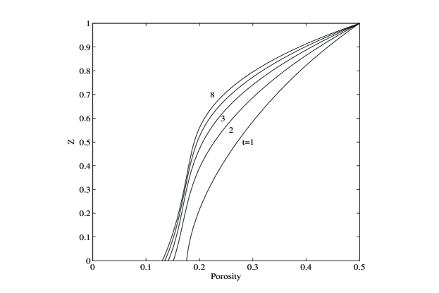
Figure 1: Poroelastic compaction profile of porosity versus rescaled height $Z=z/h(t)$ at different times $t=1,2,3,5,8$ for $\lambda=100$. Athy’s law between porosity and effective pressure is used. Porosity decreases essentially exponentially in the top region.

Figure 1 shows the poroelastic compaction profile of porosity $\phi$ versus the rescaled height $Z$ at different times $t=1,2,3,5,8$. The value of $\lambda=100$ has been used in the calculations. We can see that porosity decreases quite dramatically at the top, and profile is nearly exponential versus the rescaled depth $1-Z$.

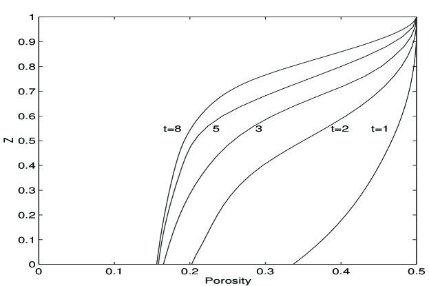
Figure 2: Viscous compaction profile of porosity versus the rescaled height $Z$. All the other parameters are the same as in Figure 1. A viscous compaction relation between effective pressure and velocity is used. The profile now is nearly parabolic.

Figure 2 provides the viscous compaction profile of porosity versus the rescaled height. All the other parameters are the same. The only difference from that of Figure 1 is that the compaction relation is now viscous. Comparing with the profile in Figure 1, it is clearly seen that porosity changes less slowly than that in the poroelastic case. The profile now is more or less parabolic. Although these two figures are quite different in the top region, there are still some similarity in the lower region, where the porosity decrease very slowly due to the fact that permeability $k(\phi)=(\phi/\phi_{0})^{m}$ is getting virtually very small as $\phi<\phi_{0}$ and $m=8$, which will in turn constrain the density-driven flow through the porous media, and thus consequently slow down the compaction process.

To understand these phenomena and to verify these numerical results, it would be very helpful if we can find some analytical solutions to be compared with. However, it is very difficulty to get general solutions for poroelastic compaction equations (24) and (25) or viscous compaction equations (28) and (29) because these equations are nonlinear with a moving boundary $h(t)$. Nevertheless, it is still possible and very helpful to find out the equilibrium state and compare with the full numerical solutions.

4.3 Equilibrium State

To find out the solutions for the equilibrium state, we must solve a nonlinear or a pair of nonlinear ordinary differential equations whose solution can usually implicitly be written in the quadrature form. In order to plot out and see the insight of the mechanism, we also need to solve these ODEs numerically although the solution procedure is straightforward. However, it is practical to get the asymptotic solutions in the explicit form in the following cases.

4.3.1 Poroelastic Compaction

For the poroelastic compaction, the equations for equilibrium state become

$$\lambda\frac{\partial}{\partial z}\{(1-\phi)(\frac{\phi}{\phi_{0}})^{m}[\frac{\partial p}{\partial z}-(1-\phi)]\}=0.$$ (35)

Substituting the expression for $p$ and integrating the above equation once together with the top boundary condition (26) gives

$$\lambda(1-\phi)^{2}(\frac{\phi}{\phi_{0}})^{m}[\frac{1}{\alpha\phi}\frac{\partial\phi}{\partial z}-1]=(\dot{m}-\dot{h})(1-\phi_{0}),$$ (36)

where we have assumed that $\dot{m}(t)=1$ and $\dot{h}=const$. The solution of this equation can be written in a quadrature although it is nonlinear.

Since $\lambda=0.01-\!\!1000$, we can expect that two distinguished limits $\lambda\rightarrow 0$ and $\lambda\rightarrow\infty$ will have very different features. For $\lambda\rightarrow 0$, we have

$$\dot{h}=\dot{m},\,\,\,\,\phi\approx\phi_{0},$$ (37)

which means that porosity does not change and no compaction occur. This corresponds to the case of very fast sedimentation or the density difference $\Delta\rho=\rho_{s}-\rho_{l}\rightarrow 0$. On the other hand, as $\lambda\rightarrow\infty$, we have

$$[\frac{1}{\alpha\phi}\frac{\partial\phi}{\partial z}-1]\approx 0,$$ (38)

its solution with the top boundary condition can be straightforwardly written as

$$\phi=\phi_{0}e^{-\alpha(h-z)},$$ (39)

which is essentially the Athy’s profile derived from real field data in sedimentary basins. Clearly, if $\alpha\rightarrow 0$ (very slow consolidation), $\phi\approx\phi_{0}$, which means that porosity changes also very slow. If $\alpha\rightarrow\infty$ (very quick consolidation), $\phi\rightarrow 0$ for $h-z>1/\alpha$, which implies that compaction proceeds so fast that the porosity is virtually zero everywhere except in a thin boundary region at the top. The thickness of the top boundary layer is approximately $1/\alpha$, which is usually $O(1)$. However, the solution (39) also satisfies the bottom boundary condition $\frac{\partial\phi}{\partial z}-\alpha\phi=0$ at $z=0$, which means that this solution is a uniformly valid solution for steady state.

4.3.2 Viscous Compaction

For the viscous compaction, the equilibrium state is governed by

$$\lambda\frac{\partial}{\partial z}\{(1-\phi)(\frac{\phi}{\phi_{0}})^{m}[\frac{\partial p}{\partial z}-(1-\phi)]\}=0,$$

$$p=\lambda\frac{\partial}{\partial z}\{(\frac{\phi}{\phi_{0}})^{m}[\frac{\partial p}{\partial z}-(1-\phi)]\},$$ (40)

The integration of the first equation together with the top boundary condition leads to

$$p=\frac{\partial}{\partial z}[\frac{(\dot{m}-\dot{h})(1-\phi_{0})}{1-\phi}],$$ (41)

and

$$\frac{(\dot{m}-\dot{h})(1-\phi_{0})}{1-\phi}=\lambda(\frac{\phi}{\phi_{0}})^{m}[(\dot{m}-\dot{h})(1-\phi_{0})\frac{\partial^{2}}{\partial z^{2}}(\frac{1}{1-\phi})-(1-\phi)],$$ (42)

whose general solution can also be written in a quadrature. However, two distinguished limits are more interesting. Clearly, if $\lambda\rightarrow 0$, we have

$$\dot{h}=\dot{m},\,\,\,\,\phi=\phi_{0},$$ (43)

which is the case of no compaction as discussed in the case of poroelastic compaction. Meanwhile, if $\lambda\rightarrow\infty$, we have

$$(\dot{m}-\dot{h})(1-\phi_{0})\frac{\partial^{2}}{\partial z^{2}}(\frac{1}{1-\phi})-(1-\phi)=0,$$ (44)

which can be rewritten as

$$(\dot{m}-\dot{h})(1-\phi_{0})\psi^{\prime\prime}-\frac{1}{\psi}=0,\,\,\,\,\psi=\frac{1}{1-\phi}.$$ (45)

By using $\psi^{\prime\prime}=\psi d\psi^{\prime}/d\psi$ and integrating from $h$ to $z$, we have

$$\frac{(\dot{m}-\dot{h})(1-\phi_{0})}{2}(\psi^{\prime})^{2}=\ln\frac{\psi}{\psi_{0}},\,\,\,\,\psi_{0}=\frac{1}{1-\phi_{0}}.$$ (46)

Further integration leads to

$$i[{\rm erf}{\frac{i}{1-\phi}}-{\rm erf}{\frac{i}{1-\phi_{0}}}]=\sqrt{\frac{2(1-\phi_{0})}{\pi(\dot{m}-\dot{h})}}(h-z).$$ (47)

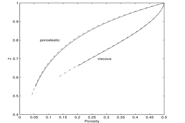
Figure 3: Comparison of asymptotic solutions (39) and (47) (dashed curves) with numerical results (solid curves) in the top region where the profile is nearly at equilibrium state. The agreement is clearly shown.

The comparison of poroelastic solution (39) and viscous solution (47) with the numerical results is shown in Figure 3 in the top region where the compaction profile is nearly at equilibrium state for $\lambda=1000$ and $t=10$. The clearly agreement verifies the numerical method and the asymptotic solution procedure.

5 Discussions

Conventional studies of compaction in porous media have focused on the separate features of poroelastic and viscous compaction. The novelty of this paper is to compare and find out distinguished features of these two different compaction styles.

Based on the pseudo-steady state approximations, the model equations of compaction can be simply written in dimensionless form as a mass conservation and Darcy’s law. A constitutive compaction relation is needed to complete this model. In the case of poro-elastic compaction, we use an Athy-type relation $\tilde{p}=\tilde{p}(\phi)$; while in the case of viscous compaction due to pressure solution creep only, we choose $\tilde{p}=-\frac{\partial u^{s}}{\partial z}$. These two different relations result in two quite different behaviours of porosity evolution. In the simpler poro-elastic case, we have a single non-linear diffusion equation for porosity $\phi$.

The analysis showed that the limit $\lambda\rightarrow 0$ (very slow compaction) can be simply analysed by means of a boundary layer analysis at the sediment base. The more interesting mathematical case is when $\lambda>>1$ (fast compaction). For sufficiently small times, the porosity profile is exponential with depth, corresponding to an equilibrium (very long time) profile. However, because of the large exponent $m$ in the permeability law $\tilde{k}=(\phi/\phi_{0})^{m}$, we find that even if $\lambda>>1$, the product $\lambda\tilde{k}$ may become small at sufficiently large depths. In this case, the porosity profile consists of an upper part near the surface where $\lambda\tilde{k}>>1$ and the equilibrium is attained, and a lower part where $\lambda\tilde{k}<<1$, and the porosity is higher than equilibrium which appears to correspond accurately to numerical computations. For the case of viscous compaction, porosity reduction occurs throughout the basin, and the basic equilibrium solution which applies near the surface is a near parabolic profile of porosity. The differences in these two profiles are very distinguished.

From the solution (39) for poroelastic compaction at equilibrium state, we see that $\phi\ll\phi_{0}$ when $\alpha(h-z)=O(1)$ or $(h-z)=O(1/\alpha)$, that is to say, the solution is significant in a region shallower than

$$\Pi_{p}\approx\frac{d}{\alpha},$$ (48)

which corresponds to a depth of 1000 m when $d\approx 1000$ m and $\alpha=1.0$. On the other hand, the viscous solution (47) only becomes significant when $\sqrt{\pi(\dot{m}-\dot{h})/2(1-\phi_{0})}=O(1)$, or in the region of depths $h-z$ greater than

$$\Pi_{v}\approx d\sqrt{\frac{\pi(\dot{m}-\dot{h})}{2(1-\phi_{0})}},$$ (49)

which is equivalent to a depth of 970 m with values of $\phi_{0}=0.5$, $\dot{m}-\dot{h}=0.3$ and $d=1000$ m. Therefore, we can generally anticipate that the poroelastic compaction is dominant in the shallow region from the surface to a depth of 1 km. At depths greater than 1 km, the pressure is high enough, pressure solution mechanism becomes significant and thus compaction is essential viscous. Naturally, there exists a region of depths near 1km where both mechanism becomes important, and an obvious extension is to include both models in a more realistic model. From the poroelastic constitutive relation (4) and viscous relation (8), we can formulate a generalised viscous-poroelastic compaction model of Maxwell type

$${\bf\nabla.u^{s}}=-\frac{1}{K_{s}}\frac{Dp_{e}}{Dt}-\frac{1}{\xi}p_{e}.$$ (50)

Subsequently, we would expect a visco-poroelastic porous medium and thus some care is needed to ensure the resulting model involving material derivatives is frame invariant. Fortunately, this frame invariance is alway true in the present 1-D formulation. Incorporation of these extension and other processes such as convection and 3-D density-driven flow will form the substance of future work.

Acknowledgements. The author wishes to thank the anonymous referees for their very helpful comments and very instructive suggestions.

References

1

I. Lerche, Basin Analysis: Quantitative Methods ( Academic Press, San Diego, California, 1990).

2

R. E. Gibson, G. L. England and M. J. L. Hussey, The Theory of One-dimensional Consolidation of Saturated Clays, I. Finite Non-linear Consolidation of Thin Homogeneous Layers, Can. Geotech. J., 17(1967)261-273.

3

D. M. Audet and A. C. Fowler, A Mathematical Model for Compaction in Sedimentary Basins, Geophys. Jour. Int., 1992, 110 (1992) 577-590.

4

A. C. Fowler and X. S. Yang, Fast and Slow Compaction in Sedimentary Basins, SIAM Jour. Appl. Math., 59(1998) 365-385.

5

J. Bear and Y. Bachmat, Introduction to Modeling of Transport Phenomena in Porous Media (Kluwer Academic, London, 1990).

6

M. A. Biot, M.A., General Theory of Three-dimensional Consolidation, J. Appl. Phys., 12 (1941) 155-164.

7

E. H. Rutter, Pressure Solution in Nature, Theory and Experiment, J. Geol. Soc. London, 140 (1976) 725-740.

8

X. S. Yang, Mathematical Modelling of Compaction and Diagenesis in Sedimentary Basins, D.Phil Thesis, Oxford University, 1997.

9

D P McKenzie, The generation and compaction of partial melts, J. Petrol., 25 (1984) 713-765.

10

A C Fowler, A compaction model for melt transport in the Earth’s asthenosphere. Part I: the basic model, in Magma Transport and Storage, ed. Ryan, M.P., John Wiley (1990) 3-14.

11

Smith, J.E., The dynamics of shale compaction and evolution in pore-fluid pressures, Math. Geol., 1971, v.3, 239-263.

12

P.C. Meek and J. Norbury, Two-Stage, Two Level Finite Difference Schemes for Non-linear Parabolic Equations, IMA J. Num. Anal., 2(1982) 335-356.