Global F-theory Models: Instantons and Gauge Dynamics

Abstract:

We elucidate certain aspects of F-theory gauge dynamics, due to quantum splitting of certain brane stacks, which are absent in the Type IIB limit. We also provide a working implementation of an algorithm for computing cohomology of line bundles on arbitrary toric varieties. This should be of general use for studying the physics of global Type IIB and F-theory models, in particular for the explicit counting of zero modes for rigid F-theory instantons which contribute to charged matter couplings. We illustrate the discussion by constructing and analyzing in detail a compact F-theory GUT model in which a D-brane instanton generates the top Yukawa coupling non-perturbatively.

1 Introduction

F-theory [1] provides a promising framework for studies of string vacua with potentially realistic particle physics. It combines many of the nice features of type IIB, particularly localization of gauge degrees of freedom on D-branes, with some of the nice features of heterotic models, such as the natural appearance of exceptional groups.

Most effort so far has centered on the classical aspects of F-theory models, i.e. couplings that can be computed as wave function overlaps. This perturbative sector is already enough for constructing appealing and phenomenologically promising models (there is a rapidly growing literature on the topic, starting with [8, 9, 10, 11]). Nevertheless, non-perturbative corrections to this picture can in some instances be the dominant contribution, and modify the picture substantially.

Classical examples come from gaugino condensation or euclidean instantons wrapping isolated cycles. Under favorable conditions [12], they can generate a superpotential for the Kähler modulus associated with the cycle. This effect has very important applications for moduli stabilization in IIB and F-theory [13, 14], and it is an essential ingredient of many semi-realistic type IIB scenarios [15].

Another important effect coming from D-brane instantons has been greatly clarified in the type II context in recent years. Whenever a D-brane instanton intersects a D-brane stack, there are some zero modes in the instanton worldvolume that are charged under the gauge symmetry on the D-brane stack. Integration over these charged zero modes can generate F-term couplings for matter fields living on the D-brane stack [16, 17, 18, 19].

In the type II context these charged instantons solve a long-standing difficulty in constructing realistic models: brane stacks have $U(1)$ factors that survive perturbatively, and generally forbid certain important couplings in the MSSM lagrangian. Typical examples are the top-quark Yukawa couplings in $SU(5)$ GUT models, and the $\mu$ term. Charged D-brane instantons do not necessarily respect perturbative $U(1)$ symmetries, and thus can generate these couplings (see [20] for a recent review).

A very attractive feature of F-theory compactifications is that, due to their close relation with exceptional groups, these $U(1)$ factors can be absent, and thus the couplings which are problematic from the type II point of view can be obtained perturbatively. Nevertheless, one may still investigate the effect of non-perturbative effects in F-theory. The motivations are many: instanton effects can be naturally suppressed, depending on the volume of the cycle wrapped by the instanton, a feature that can be quite convenient whenever one desires to obtain a hierarchy. One may also want to try a hybrid approach, building a good model in the better understood IIB context with some couplings coming from euclidean instantons and then uplifting to F-theory to improve some aspects of the model. Finally, and perhaps most importantly, non-perturbative effects will be there in any case, and one must be able to understand how they affect the model at hand.

With this motivation in mind, in this paper we discuss in detail the F-theory uplift of a particular global type IIB model in which D-brane instantons are known to play a crucial role in generating MSSM couplings, in particular the top-quark Yukawa coupling. We use this model as a prototype illustrating the two major themes of this paper: the quantum splitting of classical brane stacks, and our implementation of line bundle cohomology computations using the Čech complex. These are issues that are important for any realistic F-theoretical model building, and we are explicit about their resolution. Before going into a complete discussion, let us briefly review both issues in turn.

The first issue, quantum brane splitting, arises when uplifting interesting weakly coupled IIB models to F-theory. It can easily happen, as in our particular example, that brane stacks that make perfect sense in IIB split into sub-stacks when uplifted to F-theory. This is due to non-perturbative D$(-1)$ instantons that start modifying the geometry as soon as $g_{s}$ is non-vanishing. A convenient way of studying this problem is using D3 brane probes, for which the D$(-1)$ effects appear as ordinary gauge instantons, and the ambient geometry appears as the geometry of the Coulomb branch of moduli space. The effects of D$(-1)$ instantons on the geometry can thus be understood using Seiberg-Witten theory. We do this in section 2, explaining in which cases the quantum modification occurs, and in which it does not.

Line bundle cohomology computations arise naturally when analyzing neutral instanton zero modes, which in F-theory are counted by the cohomology groups of the trivial sheaf on the worldvolume of the instanton [12]. The framework in which we work is toric geometry, and accordingly our Calabi-Yau fourfold $Y$ will be a complete intersection in a six (complex) dimensional ambient space $X_{\Sigma^{{}^{\prime\prime}}}$, specified by toric data, with instantons wrapping divisors of $Y$. Sheaf cohomology on the instanton can then be computed by first computing the cohomology of the toric Čech complex (twisted by $\mathcal{L}$) on $X_{\Sigma^{{}^{\prime\prime}}}$, and then using the Koszul complex to project down results to divisors of $Y$. We have collected and reviewed the relevant mathematical background in section 3. The algorithm for computing Čech cohomology that we review there, while straightforward, quickly becomes intractable if done by hand. Luckily, it is not hard to instruct a computer to do it, and we provide a working implementation that should be useful for doing general computations of line bundle cohomology on arbitrary toric varieties.

Previous works on charged instantons in F-theory include [27], which lays down part of the framework required for studying charged instantons, and [28, 29], which propose to use euclidean D-branes to implement local F-theory models for GMSB (although one has to be careful in determining which instantons can be responsible for supersymmetry breaking [30, 31]).

This paper is organized as follows. In section 2 we analyze the quantum splitting of classical brane stacks, determining in which cases it occurs. In section 3 we discuss the mathematical background required for computing zero modes of instantons in the toric context, and provide the link to our implementation of the algorithm for computing Čech line bundle cohomology on toric varieties. In section 4 we illustrate these general considerations in a particular example with interesting phenomenological features.

While we were writing our results, we became aware of the work [32], which provides an efficient algorithm and computer implementation for computing line bundle cohomology on toric varieties, and thus overlaps with our discussion in section 3. We thank the authors of that work for sharing their insights.

2 F-theory Gauge Dynamics

Suppose that we are given a type IIB compactification with a stack of D7 branes. We are interested on lifting this configuration to F-theory, and in particular on the fate of the stack of D7 branes. We will see that in some cases the brane stack splits, and the F-theoretical picture is qualitatively different. For concreteness, in most of the analysis we will take the gauge group on the stack to be $SO(6)$, as that is the one that will make an appearance in our example in section 4, but the discussion generalizes easily and we give some related results at the end of our analysis.

2.1 Description from Seiberg-Witten Theory

The basic physics at play here is similar to that which smooths out the $O7^{-}$ plane in F-theory [35, 36]. It can be elucidated by studying the world-volume dynamics of a $D3$ brane probe close to the $SO(6)$ stack [37]. The theory on the worldvolume of the D3 brane has a Coulomb branch, with a Coulomb branch parameter that can be identified with the position of the D3 brane in the direction transverse to the $SO(6)$ stack. Furthermore, the exact solution of the gauge theory on the probe can be described in terms of an elliptic fibration over the Coulomb branch (the Seiberg-Witten solution [38, 39]), which can be identified with the F-theory geometry in which the probe moves [35, 36, 37].

We construct the $SO(6)$ theory by putting three D7 branes on top of an orientifold. Due to the orientifold, the worldvolume theory on the D3 brane probe is an $\mathcal{N}=2$ $SU(2)$ theory, and due to the three $A$ branes we have 3 massless quarks in the theory (at weak coupling). The Seiberg-Witten curve for the theory with three massless flavors is given by [39]:

$$y^{2}=x^{2}(x-u)+t\Lambda_{3}^{2}(x-u)^{2}$$ (1)

with $u$ the coordinate on the Coulomb branch in the $SU(2)$ theory, $\Lambda_{3}^{2}$ the strong coupling scale of the theory, and $t$ a constant which we could absorb in the definition of $\Lambda_{3}^{2}$. The elliptic fibration (1) over the complex $u$ plane degenerates over two points. There is a degeneration of order one at $u=-t\Lambda_{3}^{2}/4$, and a degeneration of order 4 at $u=0$. This already explains why we could not obtain the $SO(6)$ singularity above: the coupling $\Lambda_{3}$ of the $SU(2)$ theory is determined by the string coupling at the position of the D3. In the perturbative IIB limit this coupling is everywhere vanishing, so $\Lambda_{3}\to 0$, and the two singular points collide, enhancing the degeneration to order 5, as we expected from Tate’s classification. Nevertheless, at finite string coupling this $SO(6)$ factor decomposes into a degeneration of degree 4, and a degeneration of degree 1, separated by $\Lambda_{3}$.

Let us try to understand the physics a bit better. In order to do this it is convenient to use the classification of $(p,q)$ 7-branes described in [40, 41]. The ordinary D7-branes are of type $(1,0)$, and are denoted as $A$-type branes. An isolated $O7^{-}$ plane splits into two components in F-theory, which can be denoted as $B$ and $C$, of $(p,q)$ type $(-2,1)$ and $(0,1)$ respectively. The complete $SO(6)$ stack can then be described as a $CBAAA$ stack. We would like to understand how the five seven-branes in our stack split as we switch on a finite coupling. In order to do this, it is convenient to consider the form of the Seiberg-Witten curve for large (and equal) mass for the three flavors. It is given by [39]:

$$y^{2}=x^{2}(x-u)-\frac{1}{64}\Lambda_{3}^{2}(x-u)^{2}-\frac{3}{64}m^{2}\Lambda_{3}^{2}(x-u)+\frac{1}{4}m^{3}\Lambda_{3}x-\frac{3}{64}m^{4}\Lambda_{3}^{2}$$ (2)

As one would expect, this mass deformation separates the branes into three stacks: three branes are located at $u_{3}=m^{2}+\Lambda_{3}m/8$, and the two remaining branes are located at:

$$u_{\pm}=\frac{1}{512}\left(\Lambda_{3}^{2}-96\Lambda_{3}m\pm(\Lambda_{3}+64m)\sqrt{\Lambda_{3}^{2}+64\Lambda_{3}m}\right)$$ (3)

For large mass we can identify the branes at $u_{\pm}$ as the components of the orientifold, and the stack of three branes as the three $A$ branes. Let us now smoothly take the mass to 0. For some intermediate value of the mass the stack of three branes collides with the degeneration at $u_{+}$, and the branes can have their $(p,q)$ labels altered in the collision. After the collision the stack of three $A$ branes must become magnetic monopoles $(0,1)$ (so we recover a fourplet of monopoles in the massless regime at $u=0$ [39]), while the brane at $u_{+}$ must become a $(-1,2)$ dyon. This is indeed possible to achieve if we take the brane at $u_{+}$ to be the $B$ brane, and we take the two brane stacks to circle around each other once as they collide. We are left with $u_{-}$, which was a spectator in the whole process, and which we identify as the $C$ brane. We have depicted this process in figure 1.

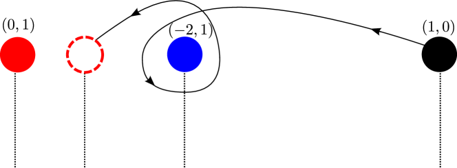
Figure 1: Schematic representation of the motion of the branes described in the text as we tune the mass parameter from large values down to 0. The red dot on the left represents the $C$ brane (of type $(0,1)$), the blue dot in the center the $B$ brane (type $(-2,1)$ before doing the monodromy), and the black dot on the right represents the stack of three $A$ branes (type $(1,0)$ before monodromy). These $A$ branes become $(0,1)$ branes after the monodromy (shown as the dashed red dot), and the $B$ brane becomes a $(-1,2)$ dyon. We have indicated the branch cuts associated with the monodromies around each brane by the dotted line.

In more detail, the process goes as follows: recall (from [40], for example) that a brane of type $(r,s)$ becomes a brane of type $(m,n)$ upon crossing the branch cut associated with a $(p,q)$ brane, with:

$$\begin{pmatrix}m\\ n\end{pmatrix}=\begin{pmatrix}1-pq&p^{2}\\ -q^{2}&1+pq\end{pmatrix}\begin{pmatrix}r\\ s\end{pmatrix}.$$ (4)

In figure 1, we have chosen conventions in in which this is the monodromy for crossing the branch cut counterclockwise. Denoting a brane of type $(p,q)$ as $X_{(p,q)}$, the sequence of crossings in figure 1 is then:

$$CBA^{3}\to CA^{3}X_{(1,1)}\to CX_{(1,1)}X_{(0,1)}^{3}\to CX_{(0,1)}^{3}X_{(-1,2)}=C^{4}X_{(-1,2)}$$ (5)

So the local geometry is simply the one obtained from putting four $C$ branes together, which gives an $SU(4)$ theory. The same result can be obtained by studying the form of (1) close to $u=0$.

Let us briefly comment on what happens in various other interesting configurations. If we tried to uplift $SO(4)$ stacks we would run into the same phenomenon. The theory to study now is $\mathcal{N}=2$ $SU(2)$ with 2 massless flavors. In this case the Seiberg-Witten curve is known to degenerate at two points, both of degree 2 [39]. Using the same arguments as above, we can argue that they correspond to a stack of two $(1,1)$ branes and a $CC$ stack. There is again a collision of stacks as we take the mass from 0 to large values, which changes the $(1,1)$ stack into an $AA$ stack, and the $CC$ stack into a couple of neighboring $B$ and $C$ branes. Similarly, lifting a $SO(2)$ stack splits the configuration into three separated degenerations of types $(1,1)$, $B$ and $C$.

One can argue in a similar fashion about what happens for most of the other classical groups: $U(N)$ stacks induce $U(1)$ dynamics on the probe, so no splitting occurs at finite coupling since the theory is abelian, and thus IR-free. $Sp(N)$ stacks induce $SO(2)$ dynamics on the probe, again non-confining. $SO(8)$ stacks give rise to a $\mathcal{N}=2$ $N_{f}=4$ $SU(2)$ theory on the probe, which is conformal, so no IR deformation of the geometry occurs. Similarly, $SO(2n)$ stacks with $n>4$ give rise to IR-free theories on the probe.

These results agree nicely with the Kodaira classification of singularities, in that the classical stacks that split quantum mechanically are exactly those that are missing from the classification. The analysis above also clarifies how some of the string junctions found in [33] for the BPS states of $\mathcal{N}=2$ $N_{f}<4$ can actually become massless in certain points in moduli space, as Seiberg-Witten theory predicts they should. As we discussed in detail above, the winding path connecting the “classical” $A^{N_{f}}BC$ description of the flavor group and the actual quantum configuration of D7 branes forces us to take the effects of $SL(2,\mathbb{Z})$ monodromy into account. It is not hard to see that the states in the classification of [33] that should become massless according to Seiberg-Witten theory, do indeed “untangle” due to the winding motion and the Hanany-Witten effect [34], and go from being involved string junctions to simple $(p,q)$-strings. These $(p,q)$ strings then become massless when the D3 collides with the D7 branes.

3 Čech Cohomology of Line Bundles over Toric Varieties

In section 4.3, we will need to perform a calculation of sheaf cohomology in order to show the absence of the $\overline{\tau}_{\dot{\alpha}}$ mode for an $O(1)$ instanton. In this section we explain in detail the steps involved in calculating such cohomologies on toric varieties, and refer the reader to a code we have written which performs such computations. For the sake of brevity, we assume that the reader is familiar with the main concepts used in the study of toric geometry, but highly recommend [21, 22, 23] for an introduction and [24, 25, 26] for a thorough treatment. For more details on Čech cohomology on toric varieties, see Chapter 9 of [25], which we follow closely here.

3.1 General Discussion

In general, the calculation of the Čech cohomology groups $\check{H}(\mathcal{U},\mathcal{F})$ for a sheaf $\mathcal{F}$ on $X$ requires knowledge of an open cover $\mathcal{U}$ of $X$, determination of the $p$th Čech cochains $\check{C}^{p}(\mathcal{U},\mathcal{F})$, and determination of the differential maps $d_{p}$, which are the maps between the Čech cochains in the Čech complex

$$0\rightarrow\check{C}^{0}(\mathcal{U},\mathcal{F})\xrightarrow{d_{0}}\check{C}^{1}(\mathcal{U},\mathcal{F})\xrightarrow{d_{1}}\dots\xrightarrow{d_{l}}\check{C}^{l-1}(\mathcal{U},\mathcal{F})\xrightarrow{d_{l-1}}\check{C}^{l}(\mathcal{U},\mathcal{F})\rightarrow\ldots$$ (6)

We will define the differentials in section 3.2 below. The $p$th Čech cochains keep track of local sections, as can be seen from the definition

$$\check{C}^{p}(\mathcal{U},\mathcal{F}) \equiv\bigoplus_{(i_{0},\dots,i_{p})\in[l]_{p}}\mathcal{F}(U_{\sigma_{i_{0}}}\cap\dots\cap U_{\sigma_{i_{p}}}),\,\,\,\,\,l=|\mathcal{U}|,$$ (7)

where $(i_{0},\dots,i_{p})\in[l]_{p}$ is a $(p+1)$-tuple of elements in the set $[l]\equiv\{1,\dots,l\}$, which has the ordering $i_{0}<\dots<i_{p}$. As $p$ increases, the sections become more and more local, and the Čech complex can be viewed intuitively as encoding how increasingly local sections “fit together”. Given this data and intuition, the $p$th Čech cohomology groups are defined to be

$$\check{H}^{p}(\mathcal{U},\mathcal{F})\equiv\frac{ker(d_{p})}{im(d_{p-1})},$$ (8)

as usual. After determining the structure of the $p$th Čech cochains and the differential maps $d_{p}$, the Čech cohomology can be computed directly as the cohomology of the complex (6).

In the generic case, however, the computation might be further complicated by not knowing, a priori, an open cover of $X$. Fortunately, in the case where $X$ is a toric variety $X_{\Sigma}$, the affine toric variety $U_{\sigma}$ associated with a cone $\sigma$ is a patch on $X_{\Sigma}$. Then there is a natural choice for an open cover, namely

$$\mathcal{U}\equiv\{U_{\sigma}\}_{\sigma\in\Sigma_{max}},\,\,\,\,\,l=|\Sigma_{max}|,$$ (9)

where $\Sigma_{max}$ is the set of top-dimensional cones. Moreover, to determine the structure of the $p$th Čech cochain in general, we must know the structure of $\mathcal{F}(U_{i_{0}}\cap\dots\cap U_{i_{p}})$, which requires knowing how the opens in $\mathcal{U}$ intersect. Again, it is a fortunate property of toric varieties that the intersection of two opens is encoded in the intersection of two cones. For example, if $\sigma_{1},\sigma_{2}\in\Sigma_{max}$ and $\tau=\sigma_{1}\cap\sigma_{2}$ is a common face, then

$$U_{\sigma_{1}}\cap U_{\sigma_{2}}=U_{\tau}.$$ (10)

Thus, for toric varieties, the relevant intersections of opens are known, and one can proceed directly to determining the structure of the Čech cochains.

The cochains we are interested in are the Čech cochains of a sheaf $\mathcal{O}_{X_{\Sigma}}(D)$ on a toric variety $X_{\Sigma}$ with the natural open cover $\mathcal{U}$ on the toric variety. On an open patch $U_{\sigma}$ associated to some cone, not necessarily top-dimensional, $\mathcal{O}_{X_{\Sigma}}(D)(U)$ is an $\mathcal{O}_{X_{\Sigma}}$-module finitely generated by the set of monomials on $U_{\sigma}$ of class $[D]$ for the divisor $D=\sum_{\rho}a_{\rho}D_{\rho}$. This just means that an arbitrary $\alpha\in\mathcal{O}_{X_{\Sigma}}(D)(U)$ is a linear combination of these monomials with coefficients that are functions on $X_{\Sigma}$. The monomials are local sections on the patch, so we write

$$\check{C}^{p}(\mathcal{\mathcal{U}},\mathcal{O}_{X_{\Sigma}}(D)) =\bigoplus_{(i_{0},\dots,i_{p})\in[l]_{p}}H^{0}(U_{\sigma_{i_{0}}}\cap\dots\cap U_{\sigma_{i_{p}}},\mathcal{O}_{X_{\Sigma}}(D)).$$ (11)

Determining the local sections of class $[D]$ is not difficult. Considering the fact that $\prod_{\rho}x_{\rho}^{a_{\rho}}$ has class $[D]$ for $x_{\rho}$ the homogeneous coordinate associated with the one-dimensional cone $\rho\in\Sigma(1)$, there is a monomial of class $[D]$ for each $m\in M$, given by

$$\prod_{\rho}x_{\rho}^{\langle m,u_{\rho}\rangle+a_{\rho}},$$ (12)

where $u_{\rho}\in N$ is the vector associated with the one-dimensional cone $\rho$ and $\langle.,.\rangle$ is the dot product. It is of class $[D]$ due to the fact that we have multiplied by a gauge invariant product of homogeneous coordinates, $\prod_{\rho}x_{\rho}^{\langle m,u_{\rho}\rangle}$.

Calculating the structure of the Čech cochains involves determining which of the monomials are well-defined on a given patch. For example, if a monomial has $\langle m,u_{\beta}\rangle<-a_{\beta}$ for $\beta\in\Sigma(1)$, then the monomial is only well defined on patches where $x_{\beta}\neq 0$. This behavior is captured in a simple way by the notion of “+” and “-” regions in the $M$ lattice, where the former is the halfplane $\langle m,u_{\beta}\rangle\geq-a_{\beta}$ and the latter is the halfplane $\langle m,u_{\beta}\rangle<-a_{\beta}$. The $M$ lattice is then partitioned by the set of lines $\langle m,u_{\rho}\rangle=-a_{\rho}\,\,\,\forall\rho\in\Sigma(1)$, where each partition is a region in the $M$ lattice categorized by a string of +’s and -’s, one for each homogeneous coordinate. For example, on $\mathbb{P}^{4}$, a lattice point $m$ in the region with sign “$-++--$” would have a corresponding monomial which is only well-defined on patches where $x_{1}$, $x_{4}$, and $x_{5}$ are non-zero. We will henceforth name such a region $R_{-++--}$, for the sake of notation. How many lattice points are in this region, or whether it exists at all, is highly dependent on the divisor $D$.

Given this intuition about local sections in terms of signed regions, we would like to relate them directly to patches $U_{\sigma}$, since we are interested in expressions of the form (11). We define

$$P_{\sigma}=\{m\in M_{\mathbb{R}}\,\,\,|\,\,\,\langle m,u_{\rho}\rangle\geq-a_{\rho},\,\,\,\forall\rho\in\sigma(1)\},$$ (13)

whose intersection with the $M$ lattice contains all lattice points $m$ whose corresponding monomials are local sections of $U_{\sigma}$. More precisely,

$$H^{0}(U_{\sigma_{i_{0}}}\cap\dots\cap U_{\sigma_{i_{p}}},\mathcal{O}_{X_{\Sigma}}(D))=\bigoplus_{m\in P_{i_{0}\dots i_{p}}\cap M}\mathbb{C}\cdot\chi^{m},$$ (14)

where $\chi^{m}$ and $P_{i_{0}\dots i_{p}}$ are shorthand for the monomial corresponding to $m$ and $P_{\sigma_{i_{0}}\cap\dots\cap\sigma_{i_{p}}}$, respectively. This identification makes sense in terms of patches, because if $m\in P_{\sigma}\cap M$, then its corresponding monomial is guaranteed to have positive exponent for the homogeneous coordinates $x_{\rho}$ for all one-dimensional cones $\rho$ in $\sigma$. This is necessary to be well-defined on $U_{\sigma}$, since $D_{\rho}=\{x_{\rho}=0\}\subseteq U_{\sigma}$, $\forall\rho\in\sigma(1)$. It is sufficient because $x_{\rho}\neq 0$ on $U_{\sigma}$ for every $\rho\notin\sigma(1)$. One should note, of course, that a given $P_{\sigma}$ is generically the union of multiple signed regions, and moreover that a given signed region might contribute to multiple $P_{\sigma}$ for different cones in the fan.

Having the requisite tools for explicitly constructing the Čech cochains, it is straightforward to compute the differentials, and one can then directly compute the Čech cohomology groups

$$\check{H}^{p}(\mathcal{U},\mathcal{O}_{X_{\Sigma}}(D))\equiv\frac{ker(d_{p})}{im(d_{p-1})}.$$ (15)

The previous discussion was general but perhaps somewhat abstract. We now proceed to illustrate how to apply these ideas in a simple but non-trivial example, $dP_{1}$. As we will see, the Čech complex gives a simple and systematic (albeit cumbersome, if done by hand) way to compute line bundle cohomology.

3.2 Calculating Čech Cohomology on $dP_{1}$

As a concrete non-trivial example, we calculate an example of Čech cohomology for a line bundle over the first del Pezzo surface, $dP_{1}$. The del Pezzo surfaces are $\mathbb{P}^{1}\times\mathbb{P}^{1}$ and the blow-up of $\mathbb{P}^{2}$ at $n$ points, $n=0,\dots,8$, which are denoted $dP_{n}$. The fan which specifies $dP_{1}$ as a toric variety is given in figure 2, and it is easy to see that the removal of $u_{4}$, which corresponds to the exceptional divisor of the blow-up, leaves us with the fan for $\mathbb{P}^{2}$. Hence, this is $dP_{1}$, also known as the first Hirzebruch surface $\mathbb{F}_{1}$.

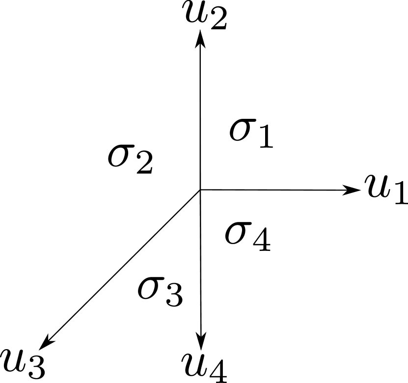
Table 1: The fan for $dP_{1}$. We have denoted the divisors $u_{i}$ and the top dimensional cones $\sigma_{i}$.

Coords	Vertices	$Q^{1}$	$Q^{2}$	Divisor Class
$x$	$u_{1}$=(1,0)	1	0	$H$
$y$	$u_{2}$=(0,1)	1	1	$H+E$
$z$	$u_{3}$=(-1,-1)	1	0	$H$
$w$	$u_{4}$=(0,-1)	0	1	$E$
$\sum_{i}[D_{i}]$		3	2	$3H+2E$

Table 2: GLSM charges for $dP_{1}$.

To fix notation, the homogeneous coordinates $x$, $y$, $z$, and $w$ are associated to the rays $u_{1}$, $u_{2}$, $u_{3}$, and $u_{4}$, respectively. For this example, we choose to calculate the Čech cohomology groups $\check{H}^{p}(\mathcal{U},\mathcal{O}_{dP_{1}}(D))$ for the divisor $D=5D_{x}-2D_{w}$. For this divisor, there are four lines which divide the $M$ lattice into signed regions, given by

$$\begin{split}l_{1}:\,\,\,m_{x}=-5,\qquad&l_{2}:\,\,\,m_{y}=0\\ l_{3}:\,\,\,m_{x}+m_{y}=0,\qquad&l_{4}:\,\,\,m_{y}=-2,\end{split}$$ (16)

which correspond to the rays $u_{1}$, $u_{2}$, $u_{3}$, and $u_{4}$, respectively. The partitioned $M$ lattice is given in figure 2, where each region has been labeled with the appropriate sign according to the conventions discussed in the previous section.

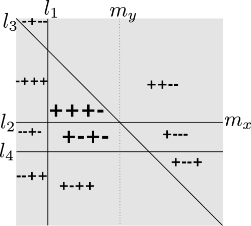
Figure 2: Signed regions in the $M$ lattice corresponding to $\mathcal{O}(5D_{x}-2D_{w})$ over $dP_{1}$. We have denoted by $m_{x}$ and $m_{y}$ the coordinate axes of the $M$ lattice.

Calculationally, rather than considering which signed regions have monomials well-defined on the intersection of a particular set of opens, it is useful to instead consider on which intersections of opens a particular monomial is well-defined. In the end, this essentially corresponds to considering the cohomological contribution of each point in the $M$ lattice. All $m$ in a given signed region will have the same contribution. This is useful since each point in the $M$ lattice contributes independently to the cohomology. In other words, there is a grading on cohomology which allows us to consider the contribution of each $m\in M$ independently. We refer the reader to chapter 9 of [25] for more details.

For this reason, we would like to categorize those $P_{\sigma}$’s which contain the $m$’s corresponding to monomials well defined on a particular intersection, as a union of signed regions. The result is

$$\begin{split}P_{1}=\bigcup R_{++\bullet\bullet}\,\,\,\,\,\,\,\,\,\,P_{2}=\bigcup R_{\bullet++\bullet}\,\,\,\,\,\,\,\,\,\,P_{3}=\bigcup R_{\bullet\bullet++}\,\,\,\,\,\,\,\,\,\,P_{4}=\bigcup R_{+\bullet\bullet+}\\ P_{12}=\bigcup R_{\bullet+\bullet\bullet}\,\,\,\,\,\,\,\,\,\,P_{13}=\bigcup R_{\bullet\bullet\bullet\bullet}\,\,\,\,\,\,\,\,\,\,P_{14}=\bigcup R_{+\bullet\bullet\bullet}\\ P_{23}=\bigcup R_{\bullet\bullet+\bullet}\,\,\,\,\,\,\,\,\,\,P_{24}=\bigcup R_{\bullet\bullet\bullet\bullet}\,\,\,\,\,\,\,\,\,\,P_{34}=\bigcup R_{\bullet\bullet\bullet+}\\ P_{123}=\bigcup R_{\bullet\bullet\bullet\bullet}\,\,\,\,\,\,\,\,\,\,P_{124}=\bigcup R_{\bullet\bullet\bullet\bullet}\,\,\,\,\,\,\,\,\,\,P_{134}=\bigcup R_{\bullet\bullet\bullet\bullet}\,\,\,\,\,\,\,\,\,\,P_{234}=\bigcup R_{\bullet\bullet\bullet\bullet}\\ P_{1234}=\bigcup R_{\bullet\bullet\bullet\bullet},\end{split}$$ (17)

where a $\bullet$ simply means that the union includes both the $+$ and the $-$ in that placeholder, so that $\cup R_{+\bullet\bullet}=R_{+++}\cup R_{++-}\cup R_{+-+}\cup R_{+--}$. This allows us to consider the contributions of a particular $m\in M$ to a Čech cochain as a vector where different entries correspond to different intersections of opens. Examples will come when we do the actual calculation.

The only technical aspect which must still be specified before actually computing the kernels and images of the differentials $d_{p}$ is the definition and form of the differentials themselves. In general, they are maps from $\check{C}^{p}(\mathcal{U},\mathcal{F})$ to $\check{C}^{p+1}(\mathcal{U},\mathcal{F})$ defined by

$$(d_{p}\sigma)_{i_{0}\dots i_{p+1}}=\sum_{k=0}^{p+1}(-1)^{k}\sigma_{i_{0}\dots\hat{i}_{l}\dots i_{p+1}}|_{U_{i_{0}}\cap\dots\cap U_{i_{p+1}}},$$ (18)

where $\hat{i}_{k}$ indicates that this index is removed. For a given set of indices $(i_{0},\dots,i_{p+1})$, this specifies one component in an element of $\check{C}^{p+1}(\mathcal{U},\mathcal{F})$. As an example, the definition (18) gives

$$(d_{1}\sigma)_{134}=\sigma_{34}|_{U_{1}\cap U_{3}\cap U_{4}}-\sigma_{14}|_{U_{1}\cap U_{3}\cap U_{4}}+\sigma_{13}|_{U_{1}\cap U_{3}\cap U_{4}}$$ (19)

for the case where $l=4$, which is our case for $dP_{1}$. Each component in an element of a Čech cochain is specified by a $(p+1)$-tuple of indices, where the components are ordered in a vector according to the natural ordering on $[l]_{p}$. Thus, equation (19) corresponds precisely to the third row in $d_{1}$, listed below.

All components of $d_{p}\sigma$ can be determined this way, which allows us to write the maps as matrices. The result in our particular case is

$$0\rightarrow\check{C}^{0}(\mathcal{U},\mathcal{O}_{dP_{1}}(5D_{x}-2D_{w}))\xrightarrow{d_{0}=\left(\scalebox{0.6}{ \begin{tabular}[]{cccc}-1&1&0&0\\ -1&0&1&0\\ 0&-1&1&0\\ 0&-1&1&0\\ 0&-1&0&1\\ 0&0&-1&0\end{tabular}}\right)} \check{C}^{1}(\mathcal{U},\mathcal{O}_{dP_{1}}(5D_{x}-2D_{w}))$$ (26)

$$\xrightarrow{d_{1}=\left(\scalebox{0.6}{ \begin{tabular}[]{ccccccc}1&-1&0&1&0&0\\ 1&0&-1&0&1&0\\ 0&1&-1&0&0&1\\ 0&0&0&1&-1&1\end{tabular}}\right)} \check{C}^{2}(\mathcal{U},\mathcal{O}_{dP_{1}}(5D_{x}-2D_{w}))$$ (31)

$$\xrightarrow{d_{2}=\left(\scalebox{0.6}{ \begin{tabular}[]{cccc}-1,1,-1,1\end{tabular}}\right)} \check{C}^{3}(\mathcal{U},\mathcal{O}_{dP_{1}}(5D_{x}-2D_{w}))\rightarrow\ldots$$ (33)

Notice that the definition of the differential, seen as a linear map between vector spaces, does not require us to specify which monomial we are dealing with. This information will only enter in the definition of the vector spaces $\check{C}^{\bullet}(\mathcal{U},\mathcal{O}_{dP_{1}}(5D_{x}-2D_{w}))$, specifying which elements of the vector space are necessarily vanishing due to the monomial under consideration not being well defined in the relevant patch.

Now all of the pieces are in place for a direct computation of cohomology. We emphasize again that it is sufficient to consider the cohomology corresponding to a given $m\in M$, and then sum over the contributions from each $m$. Moreover, since all $m$’s in a given signed region contribute to the overall cohomology in the same way, it is only necessary to compute the cohomological contributions for each signed region and to then multiply that contribution by the number of points in that region. This implies that all cohomological contributions from non-compact regions must be zero, since there are an infinite number of points, and the cohomology is finite. This means that we only need to calculate the contributions from points in $R_{+++-}$ and $R_{+-+-}$.

Let us study first the monomials in $R_{+-+-}$. From equation (17) and the natural ordering of $(p+1)$-tuples in $[l]_{p}$, elements of the Čech cochains for a given $m$ can be written

$$\begin{pmatrix}0\\ 0\\ 0\\ 0\end{pmatrix}\cdot\chi^{m}\in\check{C}^{0}(\mathcal{U},\mathcal{O}_{dP_{1}}(5D_{x}-2D_{w})),\,\,\,\,\,\begin{pmatrix}0\\ a\\ b\\ c\\ d\\ 0\end{pmatrix}\cdot\chi^{m}\in\check{C}^{1}(\mathcal{U},\mathcal{O}_{dP_{1}}(5D_{x}-2D_{w})),\,\,\,\,\,$$ (34)

$$\begin{pmatrix}e\\ f\\ g\\ h\end{pmatrix}\cdot\chi^{m}\in\check{C}^{2}(\mathcal{U},\mathcal{O}_{dP_{1}}(5D_{x}-2D_{w})),\,\,\,\,\,\begin{pmatrix}i\end{pmatrix}\cdot\chi^{m}\in\check{C}^{3}(\mathcal{U},\mathcal{O}_{dP_{1}}(5D_{x}-2D_{w})),\,\,\,\,\,$$

where $a,b,c,d,e,f,g,h,i\in\mathbb{C}$. One can then consider the action of the appropriate $d_{p}$’s on the these elements, and it is a straightforward exercise in linear algebra to show that all of the kernels and images are the same except for $im(d_{0})=0$, $ker(d_{1})=\mathbb{C}$. Thus, for each $m$ in this region, the contribution is $\check{h}^{\bullet}_{m}=(0,1,0)$.

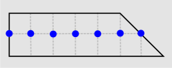
Figure 3: The only signed region which contributes to the cohomology.

In order to count points in this region recall from the definition of signed regions that “+”’s are inclusive while “-”’s are exclusive. With this in mind, only the filled dots in figure 3 contribute. Thus, the contribution of this region to the cohomology is given by

$$\check{h}^{\bullet}_{R_{+-+-}}(\mathcal{U},\mathcal{O}_{dP_{1}}(5D_{x}-2D_{w}))=(0,7,0).$$ (35)

A similar argument in the $R_{+++-}$ region shows that it does not contribute to the cohomology, and thus we conclude that

$$\check{h}^{\bullet}(\mathcal{U},\mathcal{O}_{dP_{1}}(5D_{x}-2D_{w}))=(0,7,0).$$ (36)

3.3 The Koszul Complex

Once we know the cohomology of line bundles on the ambient space, we can use an exact sequence known as the Koszul complex to obtain the cohomology on subspaces of this ambient space. Let us start with the case of induced line bundles on divisors of $\mathcal{A}$. Denoting as $N^{*}$ the dual of the normal bundle of our surface $X$ on $\mathcal{A}$, we have that:

$$0\to N^{*}\to\mathcal{O}_{\mathcal{A}}\to\mathcal{O}_{X}\to 0$$ (37)

This formula does not require that $\mathcal{A}$ is toric. In the case of a divisor $D$ of $\mathcal{A}$, $N^{*}$ is the line bundle $\mathcal{O}(-D)$. Furthermore, in order to obtain information about the cohomology of a line bundle $\mathcal{L}$ on $X$, we can tensor the whole short exact sequence above by $\mathcal{L}$, we get:

$$0\to\mathcal{O}(\mathcal{L}-D)\to\mathcal{O}_{\mathcal{A}}(\mathcal{L})\to\mathcal{O}_{X}(\mathcal{L})\to 0$$ (38)

Any short exact sequence gives rise to a long exact sequence in cohomology in a standard way. In our particular case we get:

$$\begin{split}0&\to H^{0}(\mathcal{A},\mathcal{O}(\mathcal{L}-D))\to H^{0}(\mathcal{A},\mathcal{O}(\mathcal{L}))\to H^{0}(X,\mathcal{O}(\mathcal{L}))\to\\ &\to H^{1}(\mathcal{A},\mathcal{O}(\mathcal{L}-D))\to H^{1}(\mathcal{A},\mathcal{O}(\mathcal{L}))\to H^{1}(X,\mathcal{O}(\mathcal{L}))\to\\ &\to\ldots\to H^{d}(\mathcal{A},\mathcal{O}(\mathcal{L}-D))\to H^{d}(\mathcal{A},\mathcal{O}(\mathcal{L}))\to H^{d}(X,\mathcal{O}(\mathcal{L}))\to 0\end{split}$$ (39)

where $d$ is the dimension of the ambient space.

From here we can read the dimensions of the cohomology groups. A couple of very useful facts are that we can always split any exact sequence

$$0\to A\to B\to C\to D\to\ldots$$ (40)

into two pieces:

$$0\to A\to B\to X\to 0$$ (41)

$$0\to X\to C\to D\to\ldots$$ (42)

and that for any short exact sequence $0\to A\to B\to C\to 0$ we have

$$\dim(B)=\dim(A)+\dim(C),$$ (43)

which allows one to compute the dimensions of the cohomologies in a straightforward manner.

For the case of a complete intersection of three divisors in the ambient space (our case in the main text), there is a useful general form for the Koszul complex, given by:

$$0\rightarrow\wedge^{3}N^{*}\rightarrow\wedge^{2}N^{*}\rightarrow N^{*}\rightarrow\mathcal{O}_{\mathcal{A}}\rightarrow\mathcal{O}_{D_{1}\cap D_{2}\cap D_{3}}\rightarrow 0,$$ (44)

where $N$ is the sum of the normal bundles of the divisors, $N\equiv N_{D_{1}}\oplus N_{D_{2}}\oplus N_{D_{3}}$. After splitting this sequence into short exact sequences, one uses those sequences to arrive at a number of long exact sequences in cohomology, which make it straightforward to compute the relevant groups. For the complete intersection of more hypersurfaces, the above sequence extends as one might expect.

3.4 Computer Implementation

We have implemented the algorithm described in section 3.1 using a combination of SAGE [42], C code and code from the Computational Homology Project [43].

The code and accompanying documentation can be downloaded at the web address:

http://www.sas.upenn.edu/~inaki/cech.html

4 Example: a $10\,10\,5_{H}$ Yukawa Coupling in F-theory

In this section we will illustrate the previous considerations in a particular example of phenomenological interest. The discussion is organized as follows: in section 4.1, we present the geometric data for a IIB GUT orientifold compactification on a Calabi-Yau manifold realized as a hypersurface in a toric variety. This IIB background has an euclidean D3-brane instanton generating a $10\,10\,5_{H}$ coupling. In section 4.2, we lift this IIB model to F-theory by specifying an elliptically fibered Calabi-Yau fourfold as a complete intersection in a six-dimensional toric variety. In section 4.3, we study the lifted (now M5) instanton generating the $10\,10\,5_{H}$ coupling. By an explicit line bundle cohomology computation we show the absence of fermionic zero modes that would make the contribution of the instanton to the superpotential vanish. In section 4.4, we present the precise form of the Tate sections and show that many features of the gauge $D7$ branes and $O7$ planes in IIB can be seen in the lift, but in agreement with the discussion in section 2 the $SO(6)$ gauge stack cannot be obtained at nonzero $g_{s}$.

4.1 The IIB Geometry

For the sake of reference, in this section we present the geometric data relevant for the F-theory lift of the manifold $M_{2}^{({\rm dP}_{9})^{2}}$, henceforth called $X$, which is a Calabi-Yau threefold hypersurface in a four-dimensional toric variety. It was presented in [44] as a suitable manifold for $SU(5)$ GUT model building in IIB orientifold compactifications. It exhibits many desirable features, including the generation of the $10\,10\,5_{H}$ Yukawa coupling via a euclidean $D3$ instanton.

The GLSM charges representing the ambient toric variety $X_{\Sigma}$ are given in table 3. As required by the Calabi-Yau condition, the hypersurface X has divisor class equal to the anticanonical class of the ambient toric variety, that is $\sum_{i}\,[D_{i}]$.

Coords / Vertices	$Q^{1}$	$Q^{2}$	$Q^{3}$	$Q^{4}$	Divisor Class
$x_{1}=(1,0,0,0)$	3	0	0	0	$3M$
$x_{2}=(0,1,0,0)$	2	0	0	0	$2M$
$x_{3}=(0,0,1,0)$	0	1	0	0	$N$
$x_{4}=(0,0,0,1)$	0	0	1	0	$O$
$x_{5}=(-9,-6,-1,-1)$	0	1	1	-1	$N\,+\,O\,-\,P$
$x_{6}=(-3,-2,0,0)$	1	-1	-1	-1	$M\,-\,N\,-\,O\,-\,P$
$x_{7}=(-6,-4,-1,0)$	0	0	-1	1	$-O\,+\,P$
$x_{8}=(-6,-4,0,-1)$	0	-1	0	1	$-N\,+\,P$
$\sum_{i}[D_{i}]$	6	0	0	0	$6M$

Table 3: GLSM charges for $X_{\Sigma}$, the ambient toric variety on the IIB side whose Calabi-Yau hypersurface is the threefold X. We have chosen the basis of linearly inequivalent divisors $(M,N,O,P)$ to have charges $(1,0,0,0),(0,1,0,0),(0,0,1,0),(0,0,0,1)$ under the indicated $\mathbb{C}^{*}$ gauge symmetries $Q^{i}$ of the GLSM. We have also indicated next to each field $x_{i}$ the corresponding one-dimensional generator of the fan.

In addition to this information, the orientifold involution $\sigma$ is taken to be

$$\sigma:\,\,\,x_{3}\mapsto-x_{3},$$ (45)

under which the divisors $D_{3}$ and $D_{7}$ are fixed. This identifies them as $O7$-planes, so that $[O7]=[D_{3}]+[D_{7}]$. Furthermore, via projective equivalences it can be seen that the points $x_{5}=x_{6}=x_{8}=0$ and $x_{1}=x_{5}=x_{8}=0$ are fixed points of the $\sigma$-action, and thus are the locations of $O3$-planes.

The intersection ring on the base can be computed using standard techniques of algebraic geometry. In order to talk sensibly about intersections we need to give a triangulation of the fan, or equivalently the Stanley-Reisner ideal (loosely speaking, the set of monomials in which not all terms can vanish simultaneously). We choose the following simplicial triangulation:

$$\begin{split}[[1,2,3,4],[1,2,3,8],[1,2,4,7],[1,2,5,7],[1,2,5,8],[1,3,4,6],\\ [1,3,6,8],[1,4,6,7],[1,5,6,7],[1,5,6,8],[2,3,4,6],[2,3,6,8],\\ [2,4,6,7],[2,5,6,7],[2,5,6,8]]\end{split}$$ (46)

where the integers refer to generators of the fan (so $n$ stands for $x_{n}$). The corresponding Stanley-Reisner ideal is

$$SRI=\{x_{3}x_{5},x_{3}x_{7},x_{4}x_{5},x_{4}x_{8},x_{7}x_{8},x_{1}x_{2}x_{6}\},$$ (47)

which can be seen directly from the triangulation. For example, since there is no cone in the triangulation with both $3$ and $5$, we know that $x_{3}x_{5}$ is in the Stanley-Reisner ideal.

In fact, this variety was analyzed in [44] using a different base of divisors. We can just take the result quoted there and change the base to our $M,N,O,P$ cycles. The change of base is the following:

$$\begin{split}M&=\frac{1}{2}D_{2}=3D_{5}+D_{6}+2D_{7}+2D_{8}\\ N&=D_{3}=D_{5}+D_{7}\\ O&=D_{4}=D_{5}+D_{8}\\ P&=N+O-D_{5}=D_{5}+D_{7}+D_{8}\end{split}$$ (48)

Here we have defined the basic divisors $D_{i}$ as the ones given by $x_{i}=0$, and we have used the linear equivalences of divisors:

$$\begin{split}D_{1}&=9D_{5}+3D_{6}+6D_{7}+6D_{8}\\ D_{2}&=6D_{5}+2D_{6}+4D_{7}+4D_{8}\\ D_{3}&=D_{5}+D_{7}\\ D_{4}&=D_{5}+D_{8}\end{split}$$ (49)

Using this change of basis, and the intersection form given in [44]:

$$I_{X}=D_{6}(7D_{6}^{2}-D_{5}^{2}-D_{7}^{2}-D_{8}^{2}-D_{5}D_{6}-D_{6}D_{7}-D_{6}D_{8}+D_{5}D_{7}+D_{5}D_{8})$$ (50)

we can easily obtain the triple intersection form in terms of $M,N,O,P$. The result is:

$$I_{X}=M(7M^{2}+2MN+2MO+3MP+NO+NP+OP+PP)$$ (51)

4.2 The Uplift to F-theory

In this section we present the lift of the IIB orientifold model to F-theory, where the geometry is that of an elliptically fibered Calabi-Yau fourfold $Y$ of the form

$$T^{2}\,\lhook\joinrel\relbar\joinrel\rightarrow Y\,\relbar\joinrel\twoheadrightarrow X/\sigma.$$ (52)

We follow the prescription of [45, 46, 47], which is generalizable to many lifts of IIB orientifolds, and discuss the details of this particular lift. We construct first the base of the elliptic fibration $X/\sigma$ as a hypersurface in a new ambient toric variety $X_{\Sigma^{{}^{\prime}}}$, with homogeneous coordinates whose GLSM charges have been changed relative to their counterparts in $X_{\Sigma}$ to account for modding out by the orientifold action. We then determine the divisor class of the hypersurface $X/\sigma$ and use it to calculate the canonical bundle of the base, $K_{X/\sigma}$, which is crucial in determining the precise form of the Tate sections $a_{n}$. Next, having relevant knowledge of the fourfold base, we construct a six-dimensional toric variety $X_{\Sigma^{{}^{\prime\prime}}}$, in which the Calabi-Yau fourfold $Y$ is a complete intersection of two hypersurfaces, one for the base and one for the fiber. The GLSM charges for the homogeneous coordinates of the base carry over from the toric variety $X_{\Sigma^{{}^{\prime}}}$, and we show how to determine the GLSM charges for the fiber-related coordinates $x$, $y$, and $z$ from the Weierstrass equation. We also briefly mention how one could arrive at the ambient toric variety of the fourfold $X_{\Sigma^{{}^{\prime\prime}}}$ without explicitly constructing the intermediate toric variety $X_{\Sigma^{{}^{\prime}}}$.

The Base of $Y$

Since we would like to stay in the framework of toric geometry, we will start by constructing a toric ambient space for the base. Specifically, the Calabi-Yau threefold $X$ on the IIB side is a hypersurface in the toric variety $X_{\Sigma}$, so that one can construct the base of the fourfold by modding out by the orientifold action, giving a new toric ambient space $X_{\Sigma^{{}^{\prime}}}$, and by mapping the hypersurface constraints appropriately. This requires a map from $X_{\Sigma}$ to $X_{\Sigma^{{}^{\prime}}}$ which is $2$-to-$1$ away from the $O7$-planes and $1$-to-$1$ on them. We choose the map to be

$$(x_{1},x_{2},x_{3},x_{4},x_{5},x_{6},x_{7},x_{8})\mapsto(x_{1},x_{2},x_{3}^{2},x_{4},x_{5},x_{6},x_{7}^{2},x_{8})$$ (53)

$$\equiv(\tilde{x}_{1},\tilde{x}_{2},\tilde{x}_{3},\tilde{x}_{4},\tilde{x}_{5},\tilde{x}_{6},\tilde{x}_{7},\tilde{x}_{8}),$$

where the latter are the homogeneous coordinates of $X_{\Sigma^{{}^{\prime}}}$. The effect of such a map is a simple doubling of the GLSM charges of $\tilde{x}_{3}$ and $\tilde{x}_{7}$ relative to $x_{3}$ and $x_{7}$, while the charges of the other $\tilde{x}_{i}$ are left unchanged. This is sufficient to determine the toric data of $X_{\Sigma^{{}^{\prime}}}$ presented in table 4.

Coords/Vertices	$Q^{1}$	$Q^{2}$	$Q^{3}$	$Q^{4}$	Divisor Class
$\tilde{x}_{1}=(1,0,0,0)$	3	0	0	0	$3I$
$\tilde{x}_{2}=(0,1,0,0)$	2	0	0	0	$2I$
$\tilde{x}_{3}=(0,0,1,0)$	0	2	0	0	$2J$
$\tilde{x}_{4}=(0,0,0,1)$	0	0	1	0	$K$
$\tilde{x}_{5}=(-9,-6,-2,-1)$	0	1	1	-1	$J\,+\,K\,-\,L$
$\tilde{x}_{6}=(-3,-2,0,0)$	1	-1	-1	-1	$I\,-\,J\,-\,K\,-\,L$
$\tilde{x}_{7}=(-3,-2,-1,0)$	0	0	-2	2	$-2K\,+\,2L$
$\tilde{x}_{8}=(-6,-4,0,-1)$	0	-1	0	1	$-J\,+\,L$
$\sum_{i}[\tilde{D}_{i}]$	6	1	-1	1	$6I\,+\,J\,-\,K\,+\,L$

Table 4: GLSM Charges for $X_{\Sigma^{{}^{\prime}}}$, the four-dimensional ambient toric variety for the base $X/\sigma$ of the elliptic fibration on the F-theory side. We have indicated the generators of the fan.

Having deduced the GLSM charges for the homogeneous coordinates $\tilde{x}_{i}$ in $X_{\Sigma^{{}^{\prime}}}$, we must also deduce the divisor class of $X/\sigma$. To this end, the divisor class of $X$ in $X_{\Sigma}$ is $\sum_{i}[D_{i}]=6I$. Monomials of this divisor class in $X_{\Sigma}$ get mapped to monomials of base coordinates in $X_{\Sigma^{{}^{\prime}}}$ via the map (53), from which we can read off the divisor class of $X/\sigma$ in $X_{\Sigma^{{}^{\prime}}}$. For example, from

$$x_{5}^{18}\,x_{6}^{6}\,x_{7}^{12}\,x_{8}^{12}\,\mapsto\,\tilde{x}_{5}^{18}\,\tilde{x}_{6}^{6}\,\tilde{x}_{7}^{6}\,\tilde{x}_{8}^{12}$$ (54)

we see that $X/\sigma$ has class $6I$. From this, the anticanonical bundle of the base can be computed from the adjunction formula to be $\overline{K}_{X/\sigma}=c_{1}(T_{X/\sigma})=\sum_{i}\tilde{D}_{i}-6I=J-K+L$. Thus, we see that $X/\sigma$ is not Calabi-Yau.

At this point, one could explicitly construct the Tate form of the elliptic fibration, since it is specified by sections $a_{n}\in H^{0}(X/\sigma,K_{X/\sigma}^{-n})$, and we have calculated the divisor class of the anticanonical bundle. This method was employed in [47] and was fruitful in examining the gauge enhancements associated with fiber degenerations. However, since we are interested in counting instanton zero modes via cohomologies of a divisor wrapped by a vertical $M5$ brane, it is useful to construct the full elliptically fibered fourfold $Y$ as a complete intersection in a toric ambient space. In doing so, we will be able to apply the algorithm descibed in section 3 in a straightforward manner.

The Elliptically-Fibered Fourfold Y

The process of constructing the ambient toric variety $X_{\Sigma^{{}^{\prime\prime}}}$ of the fourfold $Y$ is fairly intuitive, as one might expect, and essentially amounts to appropriately adding homogeneous coordinates for the fiber. In addition, since we wish to realize the fourfold as a complete intersection

$$Y\equiv\{P_{X/\sigma}=0\}\cap\{P_{T^{2}}=0\},$$ (55)

we must specify the divisor class of the polynomials $P_{X/\sigma}$ and $P_{T^{2}}$. The polynomial $P_{T^{2}}$ is usually chosen to be in either the Weierstrass form or (equivalently) the Tate form for an elliptic curve. For ease in determining the relevant GLSM data, we will use the Weierstrass form in this section, but will later move to the Tate form to make the determination of gauge enhancements more tractable. There is no technical difference, of course, since the Tate sections determine $f$ and $g$. We merely choose one or the other based on what is easiest for the particular task at hand.

Beginning with the base, the GLSM charges for the homogeneous coordinates in $X_{\Sigma^{{}^{\prime}}}$ carry over directly to $X_{\Sigma^{{}^{\prime\prime}}}$, with the addition of the fact that they are uncharged under the GLSM charge associated with the fiber, $Q^{5}$. We immediately know that $[P_{X/\sigma}]=6I$, since it is must have the same divisor class as $X/\sigma$ in $X_{\Sigma^{{}^{\prime}}}$.

In addition to the polynomial $P_{X/\sigma}$, we must take into account a polynomial $P_{T^{2}}$ corresponding to the elliptic fiber. As mentioned above, in this section we choose the form

$$P_{T^{2}}\equiv y^{2}-x^{3}-fxz^{4}-gz^{6},$$ (56)

the vanishing locus of which gives an elliptic curve in Weierstrass form, where $f$ and $g$ are global sections $f\in H^{0}(X/\sigma,K_{X/\sigma}^{-4})$ and $g\in H^{0}(X/\sigma,K_{X/\sigma}^{-6})$. In the case where $f$ and $g$ are merely complex numbers, rather than sections, the Weierstrass equation can be considered to be a degree six hypersurface in $\mathbb{P}_{2,3,1}$. This gives the charges $Q^{5}$ of $x$, $y$, and $z$ under the projective scaling associated only to the fiber coordinates. Moreover, from homogeneity of the Weierstrass equation, the classes $[D_{x}]$ and $[D_{y}]$ can be determined as

$$2[D_{y}]=3[D_{x}]=[g]+6[D_{z}],$$ (57)

where we use $[g]=6[\overline{K}_{X/\sigma}]=6J-6K+6L$. In addition, since we have two equations and three unknowns, we choose $[D_{z}]=M$, so that it does not transform under projective scalings of the base. This is sufficient to determine the toric data of $X_{\Sigma^{{}^{\prime\prime}}}$ presented in table 5.

Coords / Vertices	$Q^{1}$	$Q^{2}$	$Q^{3}$	$Q^{4}$	$Q^{5}$	Divisor Class
$\tilde{x}_{1}=(1,0,0,0,0,0)$	3	0	0	0	0	$3I$
$\tilde{x}_{2}=(0,1,0,0,0,0)$	2	0	0	0	0	$2I$
$\tilde{x}_{3}=(0,0,1,0,0,0)$	0	2	0	0	0	$2J$
$\tilde{x}_{4}=(0,0,0,1,0,0)$	0	0	1	0	0	$K$
$\tilde{x}_{5}=(0,0,0,0,1,0)$	0	1	1	-1	0	$J\,+\,K\,-\,L$
$\tilde{x}_{6}=(-3,-2,0,0,0,0)$	1	-1	-1	-1	0	$I\,-\,J\,-\,K\,-\,L$
$\tilde{x}_{7}=(6,4,1,1,1,0)$	0	0	-2	2	0	$-2K\,+\,2L$
$\tilde{x}_{8}=(-6,-4,0,-1,0,0)$	0	-1	0	1	0	$-J\,+\,L$
$x=(0,0,2,1,1,3)$	0	2	-2	2	2	$2J\,-\,2K\,+\,2L\,+\,2M$
$y=(-3,-2,-2,-1,-1,-2)$	0	3	-3	3	3	$3J\,-\,3K\,+\,3L\,+\,3M$
$z=(9,6,2,1,1,0)$	0	0	0	0	1	$M$
$\sum_{i}[D_{i}]$	6	6	-6	6	6	$6I\,+\,6J\,-\,6K\,+\,6L$ + 6M

Table 5: GLSM Charges for $X_{\Sigma^{{}^{\prime\prime}}}$, the six-dimensional ambient toric variety for the elliptically fibered Calabi-Yau fourfold Y, which is a complete intersection of two hypersurfaces. We have indicated the generators of the fan.

The reader should note, though, that the intermediate step of constructing the toric ambient space $X_{\Sigma^{{}^{\prime}}}$ of the base is not really necessary, since the GLSM charges of homogeneous coordinates in $X_{\Sigma^{{}^{\prime}}}$ are a subset of the GLSM charges of homogeneous coordinates in $X_{\Sigma^{{}^{\prime\prime}}}$ and one can easily deduce the charges of $y$ via the Calabi-Yau condition and the adjunction formula. This yields

$$c_{1}(T_{Y}) =c_{1}(T_{X_{\Sigma^{{}^{\prime\prime}}}})-N_{P_{X/\sigma}}-N_{P_{T^{2}}}$$ (58)

$$=\sum_{i}[D_{i}]-6I-2[D_{y}]=6J-6K+6L+6M-2[D_{y}]=0,$$

with Poincaré duality implied. In the same way, one could determine the charges of $x$, and again one could choose $z$ to only be charged under $Q^{5}$. It is then possible to read off the class of $f$ and $g$, or equivalently the Tate sections $a_{n}$, from the homogeneity of $P_{T^{2}}$, without ever explicitly calculating the anticanonical bundle. Of course, these different viewpoints are all closely tied together, and the method one uses is a matter of preference.

4.3 Instanton Zero Modes

So far, we have focused on discussing the F-theory model which will have non-perturbative corrections to the $10\,10\,5_{H}$ Yukawa coupling, but we have not yet discussed in detail the properties of the instanton which generates the coupling. The reason for this is that most known properties of euclidean branes in F-theory are known only from the properties of the relevant instanton in the IIB model.

Charged zero modes in particular, which are the ones ultimately responsible for generating the Yukawa coupling, are still poorly understood from a purely F-theoretical point of view. What we have in mind when making this statement is the description of F-theory as M-theory with vanishing fiber. The properties of charged zero modes on the euclidean M5 are not well understood. Nevertheless, F-theory is also IIB at strong coupling, and in simple situations like ours the description in terms of euclidean D3 branes is still expected to be mostly correct. See, for example, [27] for a recent paper which takes this viewpoint, obtaining a number of rules for the spectrum of charged modes (these agree with the ones obtained in IIB, except in the case where exceptional degenerations of the fiber appear).

What this means, in practice, is that the known computation of the superpotential coupling is isomorphic to the one done in IIB, except for the issue of saturation of neutral zero modes ($\bar{\tau}$ modes in particular). In this case there are more intrinsic ways of determining this spectrum. The most well known way is using Witten’s characterization of fermionic zero modes as elements of the cohomology of the structure sheaf of the divisor [12]. In the rest of this section we will use this representation, together with the result in [27] that the $\bar{\tau}$ mode can be identified with an element of $H^{0,1}(\mathcal{D})$, to argue that the $\bar{\tau}$ modes are projected out in our context. Before going into that, we would also like to mention that one can also understand the absence of dangerous neutral fermionic modes using the strongly coupled IIB viewpoint [31], so we already know what the answer should be. Nevertheless, computing the cohomology is an instructive exercise, to which we now proceed.

We study an $M5$ brane instanton on the fourfold divisor $\mathcal{D}=D_{X/\sigma}\cap D_{T^{2}}\cap D_{5}$, which is the intersection of the base, fiber, and $D_{5}$ divisors in the ambient toric sixfold $X_{\Sigma^{{}^{\prime\prime}}}$. The presence or absence of the $\overline{\tau}_{\dot{\alpha}}$ zero modes for this instanton are determined by the sheaf cohomology group

$$H^{1}(\mathcal{D},\mathcal{O}_{\mathcal{D}}),$$ (59)

which can be related to sheaf cohomologies on $X_{\Sigma^{{}^{\prime\prime}}}$ via Koszul sequences. For toric varieties, sheaf cohomology is equivalent to the Čech cohomology groups $\check{H}^{p}(\mathcal{U},\mathcal{L})$, where $\mathcal{U}$ is an open cover and $\mathcal{L}$ is a line bundle on the toric variety. Thus, our task is to compute $\check{H}^{1}(\mathcal{U},\mathcal{O}_{\mathcal{D}})$ by calculating the Čech cohomology groups of various line bundles on $X_{\Sigma^{{}^{\prime\prime}}}$. We can do this easily using our implementation of the algorithm in section 3.

The divisor $\mathcal{D}$ is the intersection of three divisors of the sixfold, whose normal bundles are given by

$$\begin{split}N_{X/\sigma}&=\mathcal{O}(6I)\\ N_{T^{2}}&=\mathcal{O}(6J-6K+6L+6M)\\ N_{D_{5}}&=\mathcal{O}(J+K-L).\end{split}$$ (60)

One can relate these objects on the ambient toric variety to the structure sheaf on $\mathcal{D}$ via the Koszul sequence

$$0\rightarrow\wedge^{3}N^{*}\rightarrow\wedge^{2}N^{*}\rightarrow N^{*}\rightarrow\mathcal{O}_{X_{\Sigma^{{}^{\prime\prime}}}}\rightarrow\mathcal{O}_{\mathcal{D}}\rightarrow 0,$$ (61)

where $N^{*}$ is the dual of $N\equiv N_{X/\sigma}\oplus N_{T^{2}}\oplus N_{D_{5}}$. For practical purposes, we split this into three short exact sequences as

$$0 \rightarrow\wedge^{3}N^{*}\rightarrow\wedge^{2}N^{*}\rightarrow K_{1}\rightarrow 0$$ (62)

$$0 \rightarrow K_{1}\rightarrow N^{*}\rightarrow K_{2}\rightarrow 0$$

$$0 \rightarrow K_{2}\rightarrow\mathcal{O}_{X_{\Sigma^{{}^{\prime\prime}}}}\rightarrow\mathcal{O}_{\mathcal{D}}\rightarrow 0,$$

each of which gives a long exact sequence in cohomology, as outlined in section 3. Looking to the parts of the long exact sequences relevant for the immediate calculation of $H^{1}(\mathcal{D},\mathcal{O}_{\mathcal{D}})$, we have

$$\dots\rightarrow H^{1} (X_{\Sigma^{{}^{\prime\prime}}},\mathcal{O}_{X_{\Sigma^{{}^{\prime\prime}}}})\rightarrow H^{1}(\mathcal{D},\mathcal{O}_{\mathcal{D}})\rightarrow H^{2}(X_{\Sigma^{{}^{\prime\prime}}},K_{2})\rightarrow H^{2}(X_{\Sigma^{{}^{\prime\prime}}},\mathcal{O}_{X_{\Sigma^{{}^{\prime\prime}}}})\rightarrow\dots$$

$$\dots\rightarrow H^{2}(X_{\Sigma^{{}^{\prime\prime}}},N^{*})\rightarrow H^{2}(X_{\Sigma^{{}^{\prime\prime}}},K_{2})\rightarrow H^{3}(X_{\Sigma^{{}^{\prime\prime}}},K_{1})\rightarrow\dots$$ (63)

$$\dots\rightarrow H^{3}(X_{\Sigma^{{}^{\prime\prime}}},\wedge^{2}N^{*})\rightarrow H^{3}(X_{\Sigma^{{}^{\prime\prime}}},K_{1})\rightarrow H^{4}(X_{\Sigma^{{}^{\prime\prime}}},\wedge^{3}N^{*})\rightarrow\dots\,\,\,,$$

one part for each short exact sequence. Calculating the cohomology of these line bundles on toric varieties, we arrive at the results

$$H^{4}(X_{\Sigma^{{}^{\prime\prime}}},\wedge^{3} N^{*})=0\,\,\,\,\,\,\,\,\,H^{3}(X_{\Sigma^{{}^{\prime\prime}}},\wedge^{2}N^{*})=0\,\,\,\,\,\,\,\,\,H^{2}(X_{\Sigma^{{}^{\prime\prime}}},N^{*})=0$$ (64)

$$H^{1}(X_{\Sigma^{{}^{\prime\prime}}},\mathcal{O}_{X_{\Sigma^{{}^{\prime\prime}}}})=0\,\,\,\,\,\,\,\,\,H^{2}(X_{\Sigma^{{}^{\prime\prime}}},\mathcal{O}_{X_{\Sigma^{{}^{\prime\prime}}}})=0,$$

where Serre duality was useful for efficiently computing $H^{4}(X_{\Sigma^{{}^{\prime\prime}}},\wedge^{3}N^{*})$. Using these results, it is easy to see that

$$H^{1}(\mathcal{D},\mathcal{O}_{\mathcal{D}})=0.$$ (65)

We see that the $\overline{\tau}_{\dot{\alpha}}$ is projected out for this instanton, as one might expect, since it is the lift of an $O(1)$ instanton in IIB. Thus, since the $\overline{\tau}_{\dot{\alpha}}$ modes are projected out and the cycle $\mathcal{D}$ is rigid, we expect an $M5$ brane instanton on $\mathcal{D}$ to give a non-perturbative correction to the $10\,10\,5_{H}$ Yukawa coupling.

As a final word, there is a technical point that may be bothering the reader: the instanton is on top of an $Sp(2)$ stack of branes, and thus the fiber degenerates everywhere over its worldvolume. From this point of view, computing the cohomology of the relevant divisor of the fourfold seems to not be well-defined. Nevertheless, with the definition that we have adopted here there are no issues, since cohomologies of line bundles on the ambient toric space are always well-defined. This point was further explored and reinforced in [27], where it was tested that the relevant cohomology does not change under blow-ups of the geometry that smooth out the degeneration of the fiber.

4.4 The Tate Form for the Uplift

In this section we discuss the details of the Tate form for the elliptic fiber in the fourfold $Y$. We construct the most general form of the sections $a_{n}$ of the Tate form in terms of the homogeneous coordinates associated with the base and show that at a point in complex structure moduli space the degenerations of the elliptic curve recover two of the three gauge groups seen in the IIB limit. We show that the third group $SO(6)$ is recovered only in Sen’s weak coupling limit. The results that we obtain in this example agree with, and illustrate, the general discussion in section 2.

The fourfold $Y$, as mentioned, is an elliptic fibration over the base $X/\sigma$. The elliptic fiber is often cast in the Weierstrass form $y^{2}=x^{3}+fxz^{4}+gz^{6}$, where $f\in H^{0}(X/\sigma;K_{X/\sigma}^{-4})$ and $g\in H^{0}(X/\sigma;K_{X/\sigma}^{-6})$ encode how the fiber varies over the base. Often more useful in practice, however, is the Tate form

$$y^{2}+a_{1}\,xyz+a_{3}\,yz^{3}=x^{3}+a_{2}\,x^{2}z^{2}+a_{4}\,xz^{4}+a_{6}\,z^{6},$$ (66)

where $a_{n}\in H^{0}(X/\sigma;K_{X/\sigma}^{-n})$ instead encode the variation of the fiber over the base. Particular combinations of the $a_{n}$’s are grouped into variables

$$b_{2}=a_{1}^{2}+4\,a_{2},\qquad b_{4}=a_{1}\,a_{3}+2a_{4},\qquad b_{6}=a_{3}^{2}+4\,a_{6}$$ (67)

which are related to $f$ and $g$ by

$$f=-{\textstyle\frac{1}{48}}(b_{2}^{2}-24\,b_{4}),\qquad g=-{\textstyle\frac{1}{864}}(-b_{2}^{3}+36b_{2}b_{4}-216\,b_{6}).$$ (68)

The discriminant, which encodes the locations of degeneration of the elliptic fiber, and thus the 7-branes, takes the form

$$\Delta_{F}=4f^{3}+27g^{2}=-{\textstyle\frac{1}{4}}\,b_{2}^{2}\,(b_{2}b_{6}-b_{4}^{2})-8b_{4}^{3}-27b_{6}^{2}+9b_{2}b_{4}b_{6}.$$ (69)

The geometry of the base determines the explicit form of the sections $a_{n}$ and the discriminant $\Delta_{F}$, from which the singularities of the fiber, and thus the corresponding gauge groups of the 7-branes, can be read off. The data relating the vanishing order of the sections $a_{n}$ and the discriminant $\Delta_{F}$ to the singularity type is reproduced in table 6.

sing.	discr.	gauge enhancement		coefficient vanishing degrees
type	$\deg(\Delta)$	type	group	${}\,\,\,\,\,\,a_{1}\quad{}$	$a_{2}$	$a_{3}$	$a_{4}$	$a_{6}{}_{\big{.}}$
$\mathrm{I}_{0}{}^{\big{.}}$	0		—	0	0	0	0	0
$\mathrm{I}_{1}$	1		—	0	0	1	1	1
$\mathrm{I}_{2}$	2	$A_{1}$	$SU(2)$	0	0	1	1	2
$\mathrm{I}_{3}^{\,\mathrm{ns}}$	3		[unconv.]	0	0	2	2	3
$\mathrm{I}_{3}^{\,\mathrm{s}}$	3		[unconv.]	0	1	1	2	3.
$\mathrm{I}_{2k}^{\,\mathrm{ns}}$	$2k$	$C_{2k}$	$SP(2k)$	0	0	$k$	$k$	$2k$.
$\mathrm{I}_{2k}^{\,\mathrm{s}}$	$2k$	$A_{2k-1}$	$SU(2k)$	0	1	$k$	$k$	$2k$
$\mathrm{I}_{2k+1}^{\,\mathrm{ns}}$	$2k+1$		[unconv.]	0	0	$k+1$	$k+1$	$2k+1$
$\mathrm{I}_{2k+1}^{\,\mathrm{s}}$	$2k+1$	$A_{2k}$	$SU(2k+1)$	0	1	$k$	$k+1$	$2k+1$.
$\mathrm{II}$	2		—	1	1	1	1	1.
$\mathrm{III}$	3	$A_{1}$	$SU(2)$	1	1	1	1	2
$\mathrm{IV}^{\,\mathrm{ns}}$	4		[unconv.]	1	1	1	2	2
$\mathrm{IV}^{\,\mathrm{s}}$	4	$A_{2}$	$SU(3)$	1	1	1	2	3
$\mathrm{I}_{0}^{*\,\mathrm{ns}}$	6	$G_{2}$	$G_{2}$	1	1	2	2	3
$\mathrm{I}_{0}^{*\,\mathrm{ss}}$	6	$B_{3}$	$SO(7)$	1	1	2	2	4
$\mathrm{I}_{0}^{*\,\mathrm{s}}$	6	$D_{4}$	$SO(8)$	1	1	2	2	4
$\mathrm{I}_{1}^{*\,\mathrm{ns}}$	7	$B_{4}$	$SO(9)$	1	1	2	3	4
$\mathrm{I}_{1}^{*\,\mathrm{s}}$	7	$D_{5}$	$SO(10)$	1	1	2	3	5
$\mathrm{I}_{2}^{*\,\mathrm{ns}}$	8	$B_{5}$	$SO(11)$	1	1	3	3	5
$\mathrm{I}_{2}^{*\,\mathrm{s}}$	8	$D_{6}$	$SO(12)$	1	1	3	3	5.
$\mathrm{I}_{2k-3}^{*\,\mathrm{ns}}$	$2k+3$	$B_{2k}$	$SO(4k+1)$	1	1	$k$	$k+1$	$2k$.
$\mathrm{I}_{2k-3}^{*\,\mathrm{s}}$	$2k+3$	$D_{2k+1}$	$SO(4k+2)$	1	1	$k$	$k+1$	$2k+1$
$\mathrm{I}_{2k-2}^{*\,\mathrm{ns}}$	$2k+4$	$B_{2k+1}$	$SO(4k+3)$	1	1	$k+1$	$k+1$	$2k+1$
$\mathrm{I}_{2k-2}^{*\,\mathrm{s}}$	$2k+4$	$D_{2k+2}$	$SO(4k+4)$	1	1	$k+1$	$k+1$	$2k+1$.
$\mathrm{IV}^{*\,\mathrm{ns}}$	8	$F_{4}$	$F_{4}$	1	2	2	3	4.
$\mathrm{IV}^{*\,\mathrm{s}}$	8	$E_{6}$	$E_{6}$	1	2	2	3	5
$\mathrm{III}^{*}$	9	$E_{7}$	$E_{7}$	1	2	3	3	5
$\mathrm{II}^{*}$	10	$E_{8}$	$E_{8}$	1	2	3	4	5
non-min	12		—	1	2	3	4	6

Table 6: Refined Kodaira classification resulting from Tate’s algorithm [57], from [58]. In order to distinguish the “semi-split” case $\mathrm{I}_{2k}^{*\,\mathrm{ss}}$ from the “split” case $\mathrm{I}_{2k}^{*\,\mathrm{s}}$ one has to work out a further factorization condition which is part of the aforementioned algorithm, see §3.1 of [58].

In our case we have $a_{n}\in H^{0}(X/\sigma;\mathcal{O}(n(J-K+L))$. Since they must be global sections, the orders of vanishing of the homogeneous coordinates $x_{i}\in X_{\Sigma^{{}^{\prime}}}$ appearing in the monomials must be positive. Thus, the divisors corresponding to the monomials must be effective:

$$[D]=\sum_{i}n_{i}[D_{i}]=n(J-K+L)\,\,\,\,\,\,\,\,n_{i}\geq 0\,\,\,\,\,\,\,\,\forall n_{i}.$$ (70)

Satisfying this condition for the case at hand yields the result

$$n_{3}=-n_{7}+n\,\,\,\,\,\,\,\,\,\,\,\,\,\,\,n_{5}=2n_{7}-n\,\,\,\,\,\,\,\,\,\,\,\,\,\,\,n_{1}=n_{2}=n_{4}=n_{6}=n_{8}=0,$$ (71)

which completely determines the allowed monomials in each section $a_{n}$. Note that this gives

$$a_{1}=c_{0}\tilde{x}_{5}\tilde{x}_{7}\,\,\,\,\,\,\,\,\,\,a_{2}=c_{1}\tilde{x}_{3}\tilde{x}_{7}+c_{2}\tilde{x}_{5}^{2}\tilde{x}_{7}^{2},$$ (72)

which leads to $b_{2}=c_{0}^{2}\tilde{x}_{5}^{2}\tilde{x}_{7}^{2}+4c_{1}\tilde{x}_{3}\tilde{x}_{7}+4c_{2}\tilde{x}_{5}^{2}\tilde{x}_{7}^{2}$. It can be shown that in Sen’s limit, the orientifold is located at $b_{2}=0$, which in our case corresponds to O7-planes on the divisor $[O7]=[D_{3}]+[D_{7}]$. This is precisely the result of the simple analysis on the IIB side. Continuing this analysis for the sake of examining possible gauge enhancements gives

$$a_{3}=c_{3}\tilde{x}_{5}^{3}\tilde{x}_{7}^{3}+c_{4}\tilde{x}_{3}\tilde{x}_{5}\tilde{x}_{7}^{2}\,\,\,\,\,\,\,\,\,\,\,\,a_{4}=c_{5}\tilde{x}_{5}^{4}\tilde{x}_{7}^{4}+c_{6}\tilde{x}_{3}\tilde{x}_{5}^{2}\tilde{x}_{7}^{3}+c_{7}\tilde{x}_{3}^{2}\tilde{x}_{7}^{2}$$ (73)

$$a_{6}=c_{8}\tilde{x}_{5}^{6}\tilde{x}_{7}^{6}+c_{9}\tilde{x}_{3}\tilde{x}_{5}^{4}\tilde{x}_{7}^{5}+c_{10}\tilde{x}_{3}^{2}\tilde{x}_{5}^{2}\tilde{x}_{7}^{4}+c_{11}\tilde{x}_{3}^{3}\tilde{x}_{7}^{3}.\,\,\,\,\,\,\,\,\,\,\,\,\,\,\,\,\,\,$$

This is the most general form for the Tate sections in this model, from which the “minimal” gauge enhancements can be read off. For example, using table 6, it can be seen from the order of vanishing along $D_{7}$ that it has minimal gauge group $G_{2}$ (a similar phenomenon was found in [20]). Rather than constructing the most general allowed fibration for this model, however, we would like to reproduce as much of the IIB physics as possible in the F-theory lift. Moving to a point in complex structure moduli space where

$$a_{2}=c_{1}\tilde{x}_{3}\tilde{x}_{7}\,\,\,\,\,\,\,\,\,\,a_{3}=4c_{1}c_{3}\tilde{x}_{3}\tilde{x}_{5}\tilde{x}_{7}^{2}\,\,\,\,\,\,\,\,\,\,a_{1}=a_{4}=a_{6}=0$$ (74)

$$\Delta_{F}=-256c_{1}^{4}c_{3}^{2}\tilde{x}_{3}^{4}\tilde{x}_{5}^{2}\tilde{x}_{7}^{7}(27c_{3}^{2}\tilde{x}_{5}^{2}\tilde{x}_{7}+c_{1}\tilde{x}_{3}),\,\,\,\,\,\,\,\,\,\,\,\,\,\,$$

it is readily seen that the gauge groups along $D_{7}$ and $D_{5}$ are $SO(10)$ and $Sp(2)$, respectively, as is the case in IIB. However, recovering the factor of $SO(6)$ along $D_{3}$ requires taking $c_{3}\to 0$, which sends $\Delta_{F}\to 0$ everywhere and thus $g_{s}\to 0$. This is precisely Sen’s limit [35]. This agrees beautifully with the discussion in section 2.

5 Conclusions

In this paper we have addressed a number of conceptual and technical issues which arise in the analysis of instanton effects in F-theory.

We started in section 2 by explaining the reason for an obstruction that can appear when trying to lift certain stacks of branes in IIB to F-theory. This also allowed us to make predictions about which IIB brane configurations are obstructed. In the process, we described in some detail the behavior of D7 branes as we go from large to vanishing flavor masses.

We continued in section 3 by discussing a way of computing sheaf bundle cohomology on toric varieties. This is essential for showing that the $\overline{\tau}_{\dot{\alpha}}$ mode is projected out, which requires calculation of the cohomology group $H^{1}(\mathcal{D},\mathcal{O}_{\mathcal{D}})$, where $\mathcal{D}$ is the fourfold divisor which the $M5$ wraps. One can compute this sheaf cohomology by calculating Čech cohomology of line bundles on the ambient toric variety, and running it through the long exact sequences in cohomology given by the splits of the Koszul sequence. Specifically, we review how to compute Čech cohomology on toric varieties in general in section 3.1 and give an illustrative example on $dP_{1}$ in section 3.2. In 3.3, we discuss the Koszul sequence, which gives a long exact sequence in cohomology which allows one to compute the cohomology $H^{1}(\mathcal{D},\mathcal{O}_{\mathcal{D}})$ by knowing information about Čech cohomology of line bundles on the ambient toric variety. Finally, in section 3.4, we provide some details about where to find our ready-to-use computer implementation of the algorithm.

In section 4 we illustrated the considerations in the previous sections in a particular example. We introduced in section 4.1 the Calabi-Yau threefold $M_{2}^{(dP_{9})^{2}}$, henceforth called $X$, as a Calabi-Yau hypersurface in a four-dimensional toric variety $X_{\Sigma}$. In section 4.2, we performed the F-theory lift of the IIB orientifold compactification on $X$, following [45]. For the sake of clarity, we presented the lift in two steps. First, we presented the fourfold base $X/\sigma$ as a hypersurface in a four-dimensional toric variety $X_{\Sigma^{{}^{\prime}}}$ by properly modding out by the orientifold action $\sigma$. Next, we presented the uplifted Calabi-Yau fourfold $Y$ as a complete intersection of two hypersurfaces in a six-dimensional toric variety $X_{\Sigma^{{}^{\prime\prime}}}$, one associated to the fiber and one to the base.

In section 4.3, we addressed the issue of instanton zero modes in the F-theory uplift of the IIB orientifold compactification on $X$. In the F-theory lift, we showed the absence of the fermionic $\overline{\tau}_{\dot{\alpha}}$ zero modes for a vertical $M5$ brane which is necessary for the generation of the $10\,10\,5_{H}$ Yukawa coupling.

In section 4.4 we determined explicitly the Tate sections and discriminant for the F-theory lift, allowing us to see the location of seven branes as divisors in the base over which the fiber degenerates, as well as their associated gauge group. At a generic point in moduli space, this data determines the “minimal” gauge enhancements along the seven branes, but we showed a point in complex structure moduli space which recovers, in F-theory, the proper location of the orientifold and two of the three gauge seven branes seen on the IIB side. Interestingly, it is only in Sen’s IIB limit that the proper enhancement of the third gauge seven brane is obtained, in agreement with the general discussion of section 2.

F-theory compactifications provide a rich field of study both for formal and phenomenological questions. The way the results in this paper came to be nicely illustrates this connection: we set out to study a particular model with some nice phenomenological features, and we were driven to fascinating questions in Seiberg-Witten theory and algebraic geometry. There is no doubt that there are still plenty of interesting phenomena to be elucidated in the quest for fully realistic F-theory models.

- [1] C. Vafa, Evidence for F-Theory, Nucl. Phys. B469 (1996) 403–418, [hep-th/9602022].
- [2] R. Blumenhagen, M. Cvetič, P. Langacker, and G. Shiu, Toward realistic intersecting D-brane models, Ann. Rev. Nucl. Part. Sci. 55 (2005) 71–139, [hep-th/0502005].
- [3] R. Blumenhagen, B. Kors, D. Lust, and S. Stieberger, Four-dimensional String Compactifications with D-Branes, Orientifolds and Fluxes, Phys. Rept. 445 (2007) 1–193, [hep-th/0610327].
- [4] M. Cvetič, J. Halverson, and R. Richter, Realistic Yukawa structures from orientifold compactifications, JHEP 12 (2009) 063, [arXiv:0905.3379].
- [5] M. Cvetič, J. Halverson, and R. Richter, Mass Hierarchies from MSSM Orientifold Compactifications, arXiv:0909.4292.
- [6] M. Cvetič, J. Halverson, and R. Richter, Mass Hierarchies vs. Proton Decay in MSSM Orientifold Compactifications, arXiv:0910.2239.
- [7] M. Cvetič, J. Halverson, P. Langacker, and R. Richter, The Weinberg Operator and a Lower String Scale in Orientifold Compactifications, arXiv:1001.3148.
- [8] R. Donagi and M. Wijnholt, Model Building with F-Theory, arXiv:0802.2969.
- [9] C. Beasley, J. J. Heckman, and C. Vafa, GUTs and Exceptional Branes in F-theory - I, JHEP 01 (2009) 058, [arXiv:0802.3391].
- [10] C. Beasley, J. J. Heckman, and C. Vafa, GUTs and Exceptional Branes in F-theory - II: Experimental Predictions, JHEP 01 (2009) 059, [arXiv:0806.0102].
- [11] R. Donagi and M. Wijnholt, Breaking GUT Groups in F-Theory, arXiv:0808.2223.
- [12] E. Witten, Non-Perturbative Superpotentials In String Theory, Nucl. Phys. B474 (1996) 343–360, [hep-th/9604030].
- [13] V. Balasubramanian, P. Berglund, J. P. Conlon, and F. Quevedo, Systematics of Moduli Stabilisation in Calabi-Yau Flux Compactifications, JHEP 03 (2005) 007, [hep-th/0502058].
- [14] F. Denef, M. R. Douglas, and B. Florea, Building a better racetrack, JHEP 06 (2004) 034, [hep-th/0404257].
- [15] S. Kachru, R. Kallosh, A. D. Linde, and S. P. Trivedi, De Sitter vacua in string theory, Phys. Rev. D68 (2003) 046005, [hep-th/0301240].
- [16] O. J. Ganor, On zeroes of superpotentials in F-theory, Nucl. Phys. Proc. Suppl. 67 (1998) 25–29.
- [17] R. Blumenhagen, M. Cvetič, and T. Weigand, Spacetime instanton corrections in 4D string vacua - the seesaw mechanism for D-brane models, Nucl. Phys. B771 (2007) 113–142, [hep-th/0609191].
- [18] L. E. Ibanez and A. M. Uranga, Neutrino Majorana masses from string theory instanton effects, JHEP 03 (2007) 052, [hep-th/0609213].
- [19] B. Florea, S. Kachru, J. McGreevy, and N. Saulina, Stringy Instantons and Quiver Gauge Theories, JHEP 05 (2007) 024, [hep-th/0610003].
- [20] R. Blumenhagen, M. Cvetič, S. Kachru, and T. Weigand, D-Brane Instantons in Type II Orientifolds, Ann. Rev. Nucl. Part. Sci. 59 (2009) 269–296, [arXiv:0902.3251].
- [21] H. Skarke, String dualities and toric geometry: An introduction, hep-th/9806059.
- [22] C. Closset, Toric geometry and local Calabi-Yau varieties: An introduction to toric geometry (for physicists), arXiv:0901.3695.
- [23] V. Bouchard, Lectures on complex geometry, Calabi-Yau manifolds and toric geometry, hep-th/0702063.
- [24] D. Cox, Lectures on toric varieties, http://www.cs.amherst.edu/~dac/lectures/coxcimpa.pdf.
- [25] D. Cox, J. Little, and H. Schenck, Toric varieties, Amer. Math. Soc. Providence, RI, to appear. http://www.cs.amherst.edu/~dac/toric.html.
- [26] W. Fulton, Introduction to toric varieties, . Princeton University Press, 1993. 157p.
- [27] R. Blumenhagen, A. Collinucci, and B. Jurke, On Instanton Effects in F-theory, arXiv:1002.1894.
- [28] J. J. Heckman, J. Marsano, N. Saulina, S. Schäfer-Nameki, and C. Vafa, Instantons and SUSY breaking in F-theory, arXiv:0808.1286.
- [29] J. Marsano, N. Saulina, and S. Schäfer-Nameki, An Instanton Toolbox for F-Theory Model Building, arXiv:0808.2450.
- [30] M. Cvetič, I. Garcia-Etxebarria, and R. Richter, 2, Branes and instantons intersecting at angles, JHEP 01 (2010) 005, [arXiv:0905.1694].
- [31] M. Cvetič, I. Garcia-Etxebarria, and R. Richter, Branes and instantons at angles and the F-theory lift of O(1) instantons, AIP Conf. Proc. 1200 (2010) 246–260, [arXiv:0911.0012].
- [32] R. Blumenhagen, B. Jurke, T. Rahn, and H. Roschy, Cohomology of Line Bundles: A Computational Algorithm, arXiv:1003.5217.
- [33] O. DeWolfe, T. Hauer, A. Iqbal, and B. Zwiebach, Constraints on the BPS spectrum of N=2, D = 4 theories with A-D-E flavor symmetry, Nucl.Phys. B534 (1998) 261–274, [hep-th/9805220].
- [34] A. Hanany and E. Witten, Type IIB superstrings, BPS monopoles, and three-dimensional gauge dynamics, Nucl.Phys. B492 (1997) 152–190, [hep-th/9611230].
- [35] A. Sen, Orientifold limit of F-theory vacua, Phys. Rev. D55 (1997) 7345–7349, [hep-th/9702165].
- [36] A. Sen, F-theory and the Gimon-Polchinski orientifold, Nucl. Phys. B498 (1997) 135–155, [hep-th/9702061].
- [37] T. Banks, M. R. Douglas, and N. Seiberg, Probing F-theory with branes, Phys. Lett. B387 (1996) 278–281, [hep-th/9605199].
- [38] N. Seiberg and E. Witten, Monopole Condensation, And Confinement In N=2 Supersymmetric Yang-Mills Theory, Nucl. Phys. B426 (1994) 19–52, [hep-th/9407087].
- [39] N. Seiberg and E. Witten, Monopoles, duality and chiral symmetry breaking in N=2 supersymmetric QCD, Nucl. Phys. B431 (1994) 484–550, [hep-th/9408099].
- [40] M. R. Gaberdiel and B. Zwiebach, Exceptional groups from open strings, Nucl. Phys. B518 (1998) 151–172, [hep-th/9709013].
- [41] O. DeWolfe and B. Zwiebach, String junctions for arbitrary Lie algebra representations, Nucl. Phys. B541 (1999) 509–565, [hep-th/9804210].
- [42] W. Stein et. al., Sage Mathematics Software (Version 4.3.4). The Sage Development Team, 2010. http://www.sagemath.org.
- [43] The CHomP Group, http://chomp.rutgers.edu.
- [44] R. Blumenhagen, V. Braun, T. W. Grimm, and T. Weigand, GUTs in Type IIB Orientifold Compactifications, Nucl. Phys. B815 (2009) 1–94, [arXiv:0811.2936].
- [45] A. Collinucci, New F-theory lifts, JHEP 08 (2009) 076, [arXiv:0812.0175].
- [46] A. Collinucci, New F-theory lifts II: Permutation orientifolds and enhanced singularities, arXiv:0906.0003.
- [47] R. Blumenhagen, T. W. Grimm, B. Jurke, and T. Weigand, F-theory uplifts and GUTs, JHEP 09 (2009) 053, [arXiv:0906.0013].
- [48] J. Marsano, N. Saulina, and S. Schafer-Nameki, F-theory Compactifications for Supersymmetric GUTs, JHEP 08 (2009) 030, [arXiv:0904.3932].
- [49] J. Marsano, N. Saulina, and S. Schafer-Nameki, Monodromies, Fluxes, and Compact Three-Generation F-theory GUTs, JHEP 08 (2009) 046, [arXiv:0906.4672].
- [50] R. Blumenhagen, T. W. Grimm, B. Jurke, and T. Weigand, Global F-theory GUTs, Nucl. Phys. B829 (2010) 325–369, [arXiv:0908.1784].
- [51] J. Marsano, N. Saulina, and S. Schafer-Nameki, Compact F-theory GUTs with , arXiv:0912.0272.
- [52] T. W. Grimm, S. Krause, and T. Weigand, F-Theory GUT Vacua on Compact Calabi-Yau Fourfolds, arXiv:0912.3524.
- [53] R. Argurio, M. Bertolini, S. Franco, and S. Kachru, Metastable vacua and D-branes at the conifold, JHEP 06 (2007) 017, [hep-th/0703236].
- [54] R. Argurio, M. Bertolini, G. Ferretti, A. Lerda, and C. Petersson, Stringy Instantons at Orbifold Singularities, JHEP 06 (2007) 067, [arXiv:0704.0262].
- [55] M. Bianchi, F. Fucito, and J. F. Morales, D-brane Instantons on the / orientifold, JHEP 07 (2007) 038, [arXiv:0704.0784].
- [56] L. E. Ibáñez, A. N. Schellekens, and A. M. Uranga, Instanton Induced Neutrino Majorana Masses in CFT Orientifolds with MSSM-like spectra, JHEP 06 (2007) 011, [arXiv:0704.1079].
- [57] J. Tate, Algorithm for determining the type of a singular fiber in an elliptic pencil, in Modular functions of one variable, IV (Proc. Internat. Summer School, Univ. Antwerp, Antwerp, 1972), pp. 33–52. Lecture Notes in Math., Vol. 476. Springer, Berlin, 1975.
- [58] M. Bershadsky et. al., Geometric singularities and enhanced gauge symmetries, Nucl. Phys. B481 (1996) 215–252, [hep-th/9605200].