Constraints on Long-Period Planets from an $L^{\prime}$ and $M$ band Survey of Nearby Sun-Like Stars: Observations

Abstract

We present the observational results of an $L^{\prime}$ and $M$ band Adaptive Optics (AO) imaging survey of 54 nearby, sunlike stars for extrasolar planets, carried out using the Clio camera on the MMT. We have concentrated more strongly than all other planet imaging surveys to date on very nearby F, G, and K stars, prioritizing stellar proximity higher than youth. Ours is also the first survey to include extensive observations in the $M$ band, which supplement the primary $L^{\prime}$ observations. Models predict much better planet/star flux ratios at the $L^{\prime}$ and $M$ bands than at more commonly used shorter wavelengths (i.e. the $H$ band). We have carried out extensive blind simulations with fake planets inserted into the raw data to verify our sensitivity, and to establish a definitive relationship between source significance in $\sigma$ and survey completeness. We find 97% confident-detection completeness for 10$\sigma$ sources, but only 46% for 7$\sigma$ sources – raising concerns about the standard procedure of assuming high completeness at 5$\sigma$, and demonstrating that blind sensitivity tests to establish the significance-completeness relation are an important analysis step for all planet-imaging surveys. We discovered a previously unknown $\sim 0.15$M_☉ stellar companion to the F9 star GJ 3876, at a projected separation of about 80 AU. Twelve additional candidate faint companions are detected around other stars. Of these, eleven are confirmed to be background stars, and one is a previously known brown dwarf. We obtained sensitivity to planetary-mass objects around almost all of our target stars, with sensitivity to objects below 3 M_Jup in the best cases. Constraints on planet populations based on this null result are presented in our Modeling Results paper, Heinze et al. (2010).

1 Introduction

Nearly 400 extrasolar planets have now been discovered using the radial velocity (RV) method. RV surveys currently have good statistical completeness only for planets with periods of less than ten years (Cumming et al., 2008; Butler et al., 2006), due to the limited temporal baseline of the observations, and the need to observe for a complete orbital period to confirm the properties of a planet with confidence. The masses of discovered planets range from just a few Earth masses (Bouchy et al., 2009) up to around 20 Jupiter masses (M_Jup). We note that a 20 M_Jup object would be considered by many to be a brown dwarf rather than a planet, but that there is no broad consensus on how to define the upper mass limit for planets. For a good overview of RV planets to date, see Butler et al. (2006) or http://exoplanet.eu/catalog-RV.php.

The large number of RV planets has enabled several good statistical analyses of planet populations (Fischer & Valenti, 2005; Butler et al., 2006; Cumming et al., 2008). However, these apply only to the short-period planets accessible to RV surveys. We cannot obtain a good understanding of planets in general without information on long period extrasolar planets; nor can we see how our own solar system fits into the big picture of planet formation in the galaxy without a good census of planets in Jupiter- and Saturn-like long-period orbits around other stars.

Several methods (transit detection, RV variations, astrometry, and direct imaging) have yielded repeatable detections of extrasolar planets so far. While RV and astrometric surveys may eventually deliver important information about long-period extrasolar planets, direct imaging is the only method that allows us to characterize them on a timescale of months rather than years or decades.

Direct imaging of extrasolar planets is technologically possible at present only in the infrared, based on the planets’ own thermal luminosity, not on reflected starlight. The enabling technology is adaptive optics (AO), which allows 6-10m ground-based telescopes to obtain diffraction limited IR images several times sharper than those from HST, despite Earth’s turbulent atmosphere. Theoretical models of giant planets indicate that such telescopes should be capable of detecting self-luminous giant planets in large orbits around young, nearby stars. The stars should be young because the glow of giant planets comes from gravitational potential energy converted to heat in their formation and subsequent contraction: lacking any internal fusion, they cool and become fainter as they age.

Several groups have published the results of AO imaging surveys for extrasolar planets around F, G, K, or M stars in the last five years (see for example Masciadri et al. (2005); Kasper et al. (2007); Biller et al. (2007); Lafrenière et al. (2007); Chauvin et al. (2010)). Of these, most have used wavelengths in the 1.5-2.2 $\mu$m range, corresponding to the astronomical $H$ and $K_{S}$ filters (Masciadri et al., 2005; Biller et al., 2007; Lafrenière et al., 2007; Chauvin et al., 2010). They have targeted mainly very young stars. Because young stars are rare, the median distance to stars in each of these surveys has been more than 20 pc.

In contrast to those above, our survey concentrates on very nearby F, G, and K stars, with proximity prioritized more than youth in the sample selection. The median distance to our survey targets is only 11.2 pc. Ours is also the first survey to include extensive observations in the $M$ band, and only the second to search solar-type stars in the $L^{\prime}$ band (the first was Kasper et al. (2007)). The distinctive focus on older, very nearby stars for a survey using longer wavelengths is natural: longer wavelengths are optimal for detecting objects with very red IR colors – that is, low temperature planets. These are most likely to be found in older systems, since planets cool and redden with age (Baraffe et al., 2003; Burrows et al., 2003). However old, low-temperature planets also have low luminosities, rendering them undetectable around all but the nearest stars.

In Section 2 we describe the criteria used in choosing our sample, and present the characteristics of our stars. In Section 3, we briefly describe our instrument, our observing strategy, and our image processing pipeline. In Section 4 we detail our sensitivity estimation methods, and show how we characterized them using blind tests in which simulated planets were inserted into our raw data – a practice that should be standard for planet imaging surveys. In Section 5 we give astrometric and photometric data for all the faint companions detected in our survey, as well as precise astrometry of the bright known binary stars in our sample. We present our conclusions in Section 6. Constraints on planet populations based on our survey null result are presented in Heinze et al. (2010).

2 The Survey Sample

The goal of our sample selection was to pick the nearest stars around which we could detect planets of 10 M_Jup or below. This practically meant that very nearby stars were potential targets up to ages of several Gyr, while at larger distances we would consider only fairly young stars. We set out initially to investigate only FGK stars within 25pc of the sun, in order to make our sample comparable in spectral type to the samples of the RV surveys, and to focus on the nearest stars, at which the $L^{\prime}$ and $M$ bands are most useful relative to shorter wavelengths. In the end we included a few M stars and a few stars slightly beyond 25pc, because these stars were very interesting and we had exhausted most of the observable stars that lay within our more strict criteria. The stars of our sample are presented in Tables 1 and 2.

Our survey focuses on markedly more nearby stars than all other surveys published to date. For example, the median distance to stars in the Masciadri et al. (2005) survey is 21.2 pc. For the Kasper et al. (2007) survey the median distance is 37 pc, for Biller et al. (2007) it is 24.7 pc, and for Lafrenière et al. (2007) it is 21.7 pc. Our median distance is 11.2 pc.

Table 1: Age, Distance, and Spectral Type of Survey Targets

	Age 1	Age 2	Adopted	Dist.	Spectral
Star	(Gyr)	(Gyr)	Age (Gyr)	(pc)	Type
GJ 5	0.11	0.2	0.155	14.25	K0Ve
HD 1405	0.1-0.2	0.03-0.08	0.100	30.00	K2V
$\tau$ Ceti	$\cdots$	$\cdots$	5.000	3.50	G8Vp
GJ 117	0.1	0.03	0.100	8.31	K2V
$\epsilon$ Eri	0.56	$\cdots$	0.560	3.27	K2V
GJ 159	0.03-0.01	$\cdots$	0.100	18.12	F6V
GJ 166 B	$\cdots$	$\cdots$	2.000	4.83	DA
GJ 166 C	$\cdots$	$\cdots$	2.000	4.83	dM4.5e
HD 29391	0.01-0.03	$\cdots$	0.100	14.71	F0V
GJ 211	0.52	$\cdots$	0.520	12.09	K1Ve
GJ 216 A	0.4-0.6	$\cdots$	0.440	8.01	F6V
BD+20 1790	0.06-0.3	$\cdots$	0.180	24.00	K3
GJ 278 C	0.1-0.3	$\cdots$	0.200	14.64	M0.5Ve
GJ 282 A	0.49	0.4-0.6	0.500	13.46	K2Ve
GJ 311	0.1	0.1-0.3	0.240	13.85	G1V
HD 77407 A	0.05	$\cdots$	0.100	30.08	G0V
HD 77407 B	0.05	$\cdots$	0.100	30.08	M2V
HD 78141	0.1-0.2	$\cdots$	0.150	21.40	K0
GJ 349	0.37	$\cdots$	0.370	11.29	K3Ve
GJ 355	0.1	0.05-0.15	0.100	19.23	K0
GJ 354.1 A	0.1	0.02-0.15	0.100	18.87	dG9
GJ 380	$\cdots$	$\cdots$	2.000	4.69	K2Ve
GJ 410	0.2-0.6	$\cdots$	0.370	11.00	dM2e
HD 96064 A	0.1-0.2	$\cdots$	0.150	24.63	G5V
HD 96064 B	0.1-0.2	$\cdots$	0.150	24.63	M3V
GJ 450	$<$1.0	$\cdots$	1.000	8.10	M1Ve
BD+60 1417	0.1-0.2	$\cdots$	0.150	17.70	K0
HD 113449	0.1-0.2	$\cdots$	0.150	22.10	G5V
GJ 505 A	0.79	$\cdots$	0.790	11.90	K2V
GJ 505 B	0.79	$\cdots$	0.790	11.90	M0.5V
GJ 519	0.2-0.6	$\cdots$	0.370	9.81	dM1
GJ 3860	0.28	0.2-0.6	0.280	14.93	K0
GJ 564	0.1-0.2	$\cdots$	0.150	17.94	G2V
GJ 3876	$\cdots$	$\cdots$	2.000	43.30	F9IV
$\xi$ Boo A	0.43	0.1	0.290	6.71	G8V
$\xi$ Boo B	0.15	$\cdots$	0.290	6.71	K4V
HD 139813	0.1-0.2	$\cdots$	0.150	21.70	G5
GJ 625	0.4-0.6	$\cdots$	0.500	6.28	dM2
GJ 659 A	$<$1.0	$\cdots$	1.000	20.20	K8V
GJ 659 B	$<$1.0	$\cdots$	1.000	20.20	dK8
GJ 684 A	0.4-0.6	$\cdots$	0.500	14.09	G0V
GJ 684 B	0.4-0.6	$\cdots$	0.500	14.09	K3V
GJ 702 A	$\cdots$	$\cdots$	2.000	5.03	K0V
GJ 702 B	$\cdots$	$\cdots$	2.000	5.03	K4V
61 Cyg A	$\cdots$	$\cdots$	2.000	3.46	K5V
61 Cyg B	$\cdots$	$\cdots$	2.000	3.46	K7V
BD+48 3686	0.1-0.2	$\cdots$	0.150	23.60	K0
GJ 860 A	$<$1.0	$\cdots$	1.000	4.01	M2V
GJ 860 B	$<$1.0	$\cdots$	1.000	4.01	M6V
GJ 879	0.1-0.3	$\cdots$	0.200	7.81	K5Ve
HD 220140 A	0.025-0.15	$\cdots$	0.100	19.74	G9V
HD 220140 B	0.025-0.15	$\cdots$	0.100	19.74	G9V
GJ 896 A	$<$0.3	$\cdots$	0.300	6.58	M3.5
GJ 896 B	$<$0.3	$\cdots$	0.300	6.58	M4.5

Note. — The adopted age, usually an average of the referenced values, is the age we used in our Monte Carlo simulations. Distances are from Perryman et al. (1997) parallaxes. For stars for which we did not have specific age estimates, we adopted an age of 2 Gyr, based on dynamical considerations setting the mean age of thin-disk stars in the solar neighborhood near this value; see Hernandez et al. (2000) and Mamajek et al. (2009). Admittedly this is a very approximate procedure, and 2 Gyr might be younger than the average age of the specific systems in question – however, these systems are not extremely important to the overall results of the survey, accounting in all for only 6.5% of the total planet detection potential, according to Table 3 of Heinze et al. (2010).

Surveying nearby, older stars at long wavelengths is interesting for several reasons. First, nearby stars offer the best chance to see planets at small physical separations, perhaps even inward to the outer limits of RV sensitivity. Second, planetary systems with ages up to several hundred Myr may still be undergoing substantial dynamical evolution due to planet-planet interactions (Juric & Tremaine, 2008; Gomes et al., 2005). While finding systems in the process of dynamical evolution would be fascinating, we also need information about systems old enough to have settled down into a mature, stable configuration. To probe long-period planet populations in mature systems, surveys such as ours that target older stars are necessary.

Additionally, theoretical spectra of older planets are likely more reliable than for younger ones, as these planets are further from their unknown starting conditions and moving toward a well-understood, stable configuration such as Jupiter’s. It has been suggested by Marley et al. (2007), in fact, that theoretical planet models such as those of Burrows et al. (2003) may overpredict the brightness of young ($<$ 100 Myr) planets by orders of magnitude, while for older planets the models are more accurate. Lastly, $L^{\prime}$ surveys such as ours and that of Kasper et al. (2007) are an important complement to the shorter-wavelength work of Masciadri et al. (2005); Biller et al. (2007); Chauvin et al. (2010); and Lafrenière et al. (2007) in that they ensure that limits on planet populations do not depend entirely on yet-untested predictions of the flux from extrasolar giant planets in a narrow wavelength interval. Until a sufficient number of extrasolar planets have been directly imaged that their spectra are well understood, surveys conducted at a range of different wavelengths will increase the confidence that may be placed in the results.

Table 2: Position and Magnitude of Survey Targets

Star	RA	DEC	V	H	K	L’
GJ 5	00:06:36.80	29:01:17.40	6.13	4.69	4.31	4.25
HD 1405	00:18:20.90	30:57:22.00	8.60	6.51	6.39	6.32
$\tau$ Ceti	01:44:04.10	-15:56:14.90	3.50	1.77	1.70	1.65
GJ 117	02:52:32.10	-12:46:11.00	6.00	4.23	4.17	4.11
$\epsilon$ Eri	03:32:55.80	-09:27:29.70	3.73	1.88	1.78	1.72
GJ 159	04:02:36.70	-00:16:08.10	5.38	4.34	4.18	4.14
GJ 166 B	04:15:21.50	-07:39:22.30	9.50	$\cdots$	$\cdots$	$\cdots$
GJ 166 C	04:15:21.50	-07:39:22.30	11.17	5.75	5.45	5.05
HD 29391	04:37:36.10	-02:28:24.80	5.22	4.77	4.54	4.51
GJ 211	05:41:20.30	53:28:51.80	6.23	3.99	4.27	4.21
GJ 216 A	05:44:27.80	-22:26:54.20	3.60	2.47	2.42	2.38
BD+20 1790	07:23:43.60	20:24:58.70	9.93	7.61	7.51	7.42
GJ 278 C	07:34:37.40	31:52:09.80	9.07	5.42	5.24	5.05
GJ 282 A	07:39:59.30	-03:35:51.00	7.20	5.06	4.89	4.82
GJ 311	08:39:11.70	65:01:15.30	5.65	4.28	4.17	4.12
HD 77407 A	09:03:27.10	37:50:27.50	7.10	5.53	5.44	5.39
HD 77407 B	09:03:27.10	37:50:27.50	$\cdots$	$\cdots$	$\cdots$	$\cdots$
HD 78141	09:07:18.10	22:52:21.60	7.99	5.92	5.78	5.72
GJ 349	09:29:54.80	05:39:18.50	7.22	5.00	4.79	4.70
GJ 355	09:32:25.60	-11:11:04.70	7.80	5.60	5.45	5.39
GJ 354.1 A	09:32:43.80	26:59:18.70	7.01	5.24	5.12	5.06
GJ 380	10:11:22.10	49:27:15.30	6.61	3.93	2.96	2.89
GJ 410	11:02:38.30	21:58:01.70	9.69	5.90	5.69	5.46
HD 96064 A	11:04:41.50	-04:13:15.90	7.64	5.90	5.80	5.75
HD 96064 B	11:04:41.50	-04:13:15.90	$\cdots$	$\cdots$	$\cdots$	$\cdots$
GJ 450	11:51:07.30	35:16:19.30	9.78	5.83	5.61	5.40
BD+60 1417	12:43:33.30	60:00:52.70	9.40	7.36	7.29	7.23
HD 113449	13:03:49.70	-05:09:42.50	7.69	5.67	5.51	5.46
GJ 505 A	13:16:51.10	17:01:01.90	6.52	4.58	4.38	4.31
GJ 505 B	13:16:51.10	17:01:01.90	9.80	5.98	5.75	5.43
GJ 519	13:37:28.80	35:43:03.90	9.07	5.66	5.49	5.28
GJ 3860	14:36:00.60	09:44:47.50	7.51	5.63	5.55	5.49
GJ 564	14:50:15.80	23:54:42.60	5.88	4.47	4.42	4.37
GJ 3876	14:50:20.40	82:30:43.00	5.64	4.19	3.92	3.87
$\xi$ Boo A	14:51:23.40	19:06:01.70	4.55	2.82	2.75	2.70
$\xi$ Boo B	14:51:23.40	19:06:01.70	6.97	4.45	4.34	4.24
HD 139813	15:29:23.60	80:27:01.00	7.31	5.56	5.46	5.41
GJ 625	16:25:24.60	54:18:14.80	10.40	6.06	5.83	5.60
GJ 659 A	17:10:10.50	54:29:39.80	8.80	6.23	6.12	5.97
GJ 659 B	17:10:12.40	54:29:24.50	9.29	6.13	5.97	5.83
GJ 684 A	17:34:59.59	61:52:28.39	5.23	3.89	3.74	$\cdots$
GJ 684 B	17:34:59.59	61:52:28.39	8.06	$\cdots$	$\cdots$	$\cdots$
GJ 702 A	18:05:27.30	02:30:00.40	4.20	2.32	2.24	2.18
GJ 702 B	18:05:27.30	02:30:00.40	6.00	3.48	3.37	3.27
61 Cyg A	21:06:53.90	38:44:57.90	5.21	2.47	2.36	2.25
61 Cyg B	21:06:55.30	38:44:31.40	6.03	3.02	2.87	2.74
BD+48 3686	22:20:07.00	49:30:11.80	8.57	6.58	6.51	6.45
GJ 860 A	22:27:59.47	57:41:45.15	9.59	5.04	4.78	$\cdots$
GJ 860 B	22:27:59.47	57:41:45.15	10.30	$\cdots$	$\cdots$	$\cdots$
GJ 879	22:56:24.10	-31:33:56.00	6.48	3.80	3.81	3.70
HD 220140 A	23:19:26.60	79:00:12.70	7.54	5.74	5.66	5.60
HD 220140 B	23:19:26.60	79:00:12.70	$\cdots$	$\cdots$	$\cdots$	$\cdots$
GJ 896 A	23:31:52.20	19:56:14.10	9.95	5.24	4.99	4.64
GJ 896 B	23:31:52.20	19:56:14.10	12.40	6.98	6.68	6.28

Note. — Coordinates are epoch J2000.0 and are mostly from Perryman et al. (1997). $H$ and $K$ magnitudes are from Cutri et al. (2003), or else calculated from Simbad website spectral types and $V$ magnitudes using Table 7.6 of Cox (2000). $L^{\prime}$ magnitudes are similarly calculated from either $V$ or $K$ values.

As can be seen from Table 1, some estimates have placed the ages of some of our stars well below 100 Myr. We have chosen to approximate these ages as 100 Myr. There are several reasons for this. First, the Burrows et al. (2003) models we have adopted do not give the type of observables we need for planets younger than 100 Myr. Second, setting the ages of these stars slightly older than they are thought to be fits in with our generally conservative approach to the volatile subject of extrasolar planet searches, and ensures that our survey results do not hang on just a few very young stars and will not be invalidated if the age estimates are revised upward. Finally, setting the ages conservatively hedges our results to some extent against the possibility suggested in Marley et al. (2007) that young massive planets may be far fainter than expected because much of the gravitational potential energy of the accreting material may get radiated away in an accretion shock and thus never get deposited in the planet’s interior. Figure 4 in Marley et al. (2007) shows that in this accretion scenario planets start out at much lower luminosities than predicted by ‘hot start’ models such as those of Burrows et al. (2003), but over time the predictions converge. By 100 Myr, the differences are less than an order of magnitude for planets less massive than 10 M_Jup, and are negligible for planets of 4 M_Jup and lower masses.

3 Observations and Image Processing

3.1 The Instrument

The Clio instrument we used for our observations has been well described elsewhere (Freed et al. (2004), Sivanandam et al. (2006), and Hinz et al. (2006)). We present only a brief overview here.

The MMT AO system delivers a lower thermal background than others because it uses the world’s first deformable secondary mirror, thereby avoiding the multiple warm-mirror reflections (each adding to the thermal background) that are needed in other AO systems. This unique property makes the MMT ideal for AO observations in wavelengths such as the $L^{\prime}$ and $M$ bands that are strongly affected by thermal glow. Clio was developed to take advantage of this to search for planets in these bands. It saw first light as a simple imager offering F/20 and F/35 modes. The design allowed for coronagrapic capability, which has since been developed (Kenworthy et al., 2007) but was not used in our survey. In the F/20 mode, which we we used for all the observations reported herein, Clio’s field of view is 15.5$\times$12.4 arcseconds. Its plate scale is $0.04857\pm 0.00003$ arcseconds per pixel, which gives finer than Nyquist sampling of the diffraction-limited point spread function (PSF) of the MMT in the $L^{\prime}$ and $M$ bands.

3.2 Observations

For each star in our sample we sought to acquire about one hour or more of cumulative integration at the $L^{\prime}$ band. In most cases we achieved this. For some of our brightest nearby targets we acquired $M$ band integrations as well. If possible we observed the star through transit, not only to minimize airmass, but also to obtain the greatest possible amount of parallactic rotation. Parallactic rotation is important because it causes image artifacts from the telescope to rotate with respect to real sources, rendering them more distinguishable. To enhance this effect, we observed with the instrument rotator off, so that rays and ghosts from the Clio instrument itself would also rotate, and could be suppressed by the same procedures that suppressed telescope artifacts (see Section 3.3).

After acquiring each target with MMTAO, we determined a single-frame integration time for our science images based solely on the sky background. This integration time was chosen so that the sky background flux filled $60-80\%$ of the detector full-well capacity. This ensured that beyond the speckle halo of the star the observations were background-limited rather than readnoise limited. The optimal integration time changed due to night-to-night variations in sky brightness, usually ranging from 1.5 to 2.0 seconds in $L^{\prime}$ and from 100-200 msec at $M$; see Table 3 for details. The science exposures generally saturated the primary star. When possible, we interleaved a few shorter exposures providing unsaturated images. These could be used later to determine the true PSF delivered by the AO system during observations of a particular star.

In normal operation Clio coadds several individual frames and saves them as a single FITS image. We used this option except for our observations of the star GJ 380, for which we saved and processed the frames individually. The increased data volume and processing runtimes for GJ 380 outweighed any minor advantages the single-frame approach may offer in terms of image quality. Coadding delivers good-quality data much more efficiently.

Table 3 shows the date on which each of our target stars was observed, the nominal single-frame integration time, the coadds, and the number of coadded FITS images we acquired. The true single-frame integration for Clio is the nominal integration plus 59.6 msec. Table 4 gives the full science integration, parallactic rotation, and mean airmass for each star.

We took our data using the standard IR imaging technique of nodding, in which a sequence of images is taken in one position, the telescopes is moved (‘nodded’) slightly, and then another image sequence is acquired. Images taken at one position can then be subtracted from images taken at the other position. In contrast to the on-source/off-source nodding used in some types of observations, we place the science target on the detector in both nod positions to maximize the useful data aquired. Artifacts of the bright sky interacting with the telescope and the detector vanish on nod subtraction, while real celestial objects, including the target star itself, appear as bright and dark images separated by a distance set by the nod amplitude (typically about half our field of view). Nodding is a powerful technique, and is practically indispensible for $L^{\prime}$ and $M$ band observations. We typically nodded the telescope every 2-5 minutes. This was short enough that alterations in the sky background did not introduce appreciable noise into our data – in sharp contrast to, e.g., 10 $\mu$m $N$ band observations, where a ‘chopping’ mirror must be used to switch between source and sky on a timescale of seconds or less.

Table 3: Observations of Science Targets: Basic Parameters

	Date Obs.
Star	(yyyy/mm/dd)	Band	Clio int(msec)	Coadds	# Images
GJ 659A	2006/04/11	L’	2000	10	90
GJ 354.1A	2006/04/12	L’	2000	10	232
GJ 450	2006/04/12	L’	2000	10	260
GJ 625	2006/04/12	L’	2000	10	208
GJ 349	2006/04/13	L’	2000	10	240
GJ 564	2006/04/13	L’	2000	10	193
GJ 3876	2006/04/13	L’	2000	25	68
GJ 3860	2006/06/09	L’	1500	15	170
HD 139813	2006/06/09	L’	1200	20	148
GJ 702 AB	2006/06/09	L’	1200	20	95
61 Cyg A	2006/06/09	L’	1200	20	133
BD+60 1417	2006/06/10	L’	1200	20	160
$\xi$ Boo AB	2006/06/10	L’	1200	20	157
61 Cyg B	2006/06/10	L’	1500	15	140
GJ 519	2006/06/10	L’	1500	15	180
BD+48 3686	2006/06/11	L’	1200	20	130
$\xi$ Boo AB	2006/06/11	M	100	100	260
GJ 684 AB	2006/06/11	L’	1200	20	120
GJ 505 AB	2006/06/11	L’	1200	20	149
GJ 659 B	2006/06/12	L’	1200	20	170
61 Cyg A	2006/06/12	M	100	100	176
GJ 860 AB	2006/06/12	L’	1200	20	104
61 Cyg B	2006/07/12	M	100	100	274
GJ 896 AB	2006/07/13	L’	1500	20	105
$\epsilon$ Eri	2006/09/09	M	130	100	180
GJ 5	2006/09/11	L’	1500	15	210
$\epsilon$ Eri	2006/09/11	L’	1500	15	184
GJ 117	2006/12/01	L’	1500	15	139
GJ 211	2006/12/01	L’	1500	15	170
GJ 282 A	2006/12/01	L’	1500	15	190
HD 1405	2006/12/02	L’	1500	15	98
GJ 159	2006/12/02	L’	1500	15	180
GJ 216 A	2006/12/02	L’	1500	15	158
GJ 278 C	2006/12/02	L’	1500	15	132
GJ 355	2006/12/02	L’	1500	15	159
GJ 879	2006/12/03	L’	1500	15	54
HD 220140 AB	2006/12/03	L’	1500	15	170
GJ 166 BC	2006/12/03	L’	1500	15	149
GJ 311	2006/12/03	L’	1500	15	90
GJ 410	2006/12/03	L’	1500	15	100
$\tau$ Ceti	2007/01/04	L’	1700	15	160
HD 29391	2007/01/04	L’	1700	15	200
BD+20 1790	2007/01/04	L’	1700	15	188
HD 96064 AB	2007/01/05	L’	1700	15	180
HD 77407 AB	2007/01/05	L’	1700	15	79
HD 78141	2007/04/11	L’	1700	15	203
HD 113449	2007/04/11	L’	1500	15	190
GJ 702 AB	2007/04/11	M	200	100	144
GJ 380	2007/04/30	L’	1500	1	2066

Note. — The ‘Clio int’ column gives the nominal single-frame integration time for Clio in msec. The actual single frame integration is 59.6 msec longer in every case.

Table 4: Observations of Science Targets: Data Acquired

Star	Band	Exposure(sec)	Mean Airmass	Rotation	Proc. Methods
GJ 659 A	L’	1853.64	1.113	15.80∘	a, b, d, e
GJ 354.1 A	L’	4778.27	1.032	130.75∘	a, b, d, e, x, y
GJ 450	L’	5354.96	1.031	110.37∘	a, b, d, e, x, y
GJ 625	L’	4283.97	1.117	45.65∘	a, b, d, e, x, y
GJ 349	L’	4943.04	1.178	40.61∘	a, b, d, e
GJ 564	L’	3975.03	1.036	70.70∘	a, b, d, e
GJ 3876	L’	3501.32	1.601	27.23∘	a, b, d, e
GJ3860	L’	3976.98	1.086	47.09∘	a, b, d, e
HD139813	L’	3728.42	1.529	30.15∘	a, b, d, e
GJ 702 AB	L’	2393.24	1.149	25.50∘	a, b, d, e, f, g
61 Cyg A	L’	3350.54	1.012	101.25∘	a, b, d, e
BD+60 1417	L’	4030.72	1.153	37.65∘	a, b, d, e
$\xi$ Boo AB	L’	3955.14	1.047	71.20∘	a, b, d, e, f, g
61 Cyg B	L’	3275.16	1.012	103.68∘	a, b, d, e
GJ 519	L’	4210.92	1.011	139.97∘	a, b, d, e
BD+48 3686	L’	3274.96	1.074	35.97∘	a, b, d, e
$\xi$ Boo AB	M	4149.60	1.060	46.142∘	a, b, d, e, f, g
GJ 684 AB	L’	3023.04	1.175	24.15∘	d, e, y, g
GJ 505 AB	L’	3753.61	1.070	45.30∘	a, b, d, e, f, g, x, y
GJ 659 B	L’	4282.64	1.112	43.93∘	a, b, d, e
61 Cyg A	M	2808.96	1.025	44.24∘	a, b, d, e
GJ 860 AB	L’	2619.97	1.133	24.55∘	a, d, e, g, y
61 Cyg B	M	4373.04	1.018	118.96∘	d, e, y
GJ 896 AB	L’	3275.16	1.026	66.49∘	a, b, d, e, f, y
$\epsilon$ Eri	M	3412.80	1.334	23.406∘	d, e, y
GJ 5	L’	4912.74	1.011	146.98∘	a, b, d, e, x, y
$\epsilon$ Eri	L’	4304.50	1.342	36.92∘	d, e, y
GJ 117	L’	3251.77	1.463	34.05∘	a, b, d, e, x, y
GJ 211	L’	3976.98	1.097	50.12∘	a, b, d, e, x, y
GJ 282 A	L’	4444.86	1.281	30.28∘	a, b, d, e, x, y
HD 1405	L’	2292.61	1.036	162.97∘	a, b, d, e, x, y
GJ 159	L’	4210.92	1.189	37.65∘	a, b, d, e, x, y
GJ 216 A	L’	3696.25	1.739	30.10∘	a, b, d, e, x, y
GJ 278 C	L’	3088.01	1.017	170.627∘	a, b, c, d, e, x, y
GJ 355	L’	3719.65	1.380	25.74∘	a, b, c, d, e, x, y
GJ 879	L’	1263.28	2.232	11.68∘	a, c, d, x, y
HD 220140 AB	L’	3976.98	1.494	14.14∘	a, b, d, e, f, g, x, y
GJ 166 BC	L’	3485.71	1.301	28.66∘	a, b, d, e, x, y
GJ 311	L’	2105.46	1.201	26.23∘	a, b, c, d, e, x, y
GJ 410	L’	2339.40	1.026	34.26∘	a, b, c, d, e, x, y
$\tau$ Ceti	L’	4223.04	1.535	37.03∘	a, b, d, e, x, y
HD 29391	L’	5278.80	1.227	39.63∘	a, b, c, d, e, x, y
BD+20 1790	L’	4962.07	1.068	47.94∘	a, b, d, e, x, y
HD 96064 AB	L’	4750.92	1.252	41.74∘	a, b, d, e, x, y
HD 77407 AB	L’	2085.13	1.008	95.44∘	a, b, c, d, e, f, g, x, y
HD 78141	L’	5297.98	1.022	109.11∘	a, b, c, d, e, x, y
HD 113449	L’	4444.86	1.263	35.36∘	a, b, d, e, x, y
GJ 702 AB	M	3738.24	1.171	32.70∘	d, e, g, y
GJ 380	L’	3222.13	1.341	20.58∘	a, b, d, e, x, y

Note. — Proc. Methods refers not to the data that were acquired, but to different methods used in processing the data. Each method represents a different master image produced by stacking the entire data set after applying a particular set of pre-stack processing algorithms. For example, four separate master images were made of the star GJ 659A. Each was a stack of all the images acquired, processed using a different method of pre-stack image processing: the ‘a’, ‘b’, ‘d’, and ‘e’ methods in the case of this star. The different processing methods are explained in Section 3.3

3.3 Image Processing

Image processing for AO planet search images tends to be complex and sophisticated. We have given a brief outline of our processing pipeline in Heinze et al. (2008), which is applicable to the current work, and we hope to detail the unique aspects of our pipeline in a separate future paper. Here we will briefly describe the processing sequence, stressing aspects that were not covered in Heinze et al. (2008), but which become more important for the larger set of stars, processed over a longer period of time, that we describe herein.

We begin the processing of each Clio image by normalizing it to a single coadd, subtracting an equal-exposure dark frame usually taken immediately before or after the science data sequence, and dividing by a flat frame. There follows an initial step of bad-pixel fixing. The next step is nod subtraction: from every image we subtract an identically processed copy of an image from the opposite nod position. This nod subtraction image is scaled (by a factor that is always very close to unity) so that its mean sky brightness exactly matches that of the science image from which it is being subtracted; the scaling is useful to compensate for small variations in sky brightness. Further bad-pixel fixing and bad-column correction follows. Finally, an algorithm to remove residual pattern noise is applied, and the image is zero-padded, shifted, and rotated in a single bicubic spline operation so that celestial north is up and the center-of-mass centroid of the primary star is located in the exact center of the image. See Figure 1 for an example of our processing sequence, applied to the nearby binary star GJ 896.

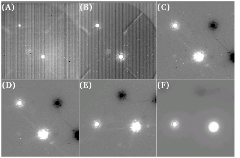
Figure 1: (A) Raw image of the nearby binary star GJ 896. (B) Same image after dark subtraction and flatfielding. Contrast stretched 5$\times$ relative to (A). (C) Same image after nod subtraction. Contrast stretched 2.5$\times$ relative to (B). (D) Same image after correction for bad pixels and bad columns. (E) Same image after shifting and rotation. (F) Final stack made from 105 images like (E). Unsharp masking has not yet been applied. The field of view for each tile is 10.6 arcsec square.

The rotation places celestial north up on the images with an accuracy of about 0.2 degrees. Since we do not use the instrument rotator, a different rotation is required for each image: the parallactic angle plus a constant offset, which we determine by observing known binary stars (this is further described in section 5.3). While parallactic rotation of bright binary stars over just tens of seconds has been detected due to the high internal precision of Clio astrometry, in no case does sufficient parallactic rotation occur during a Clio coadd sequence to appreciably blur the science images.

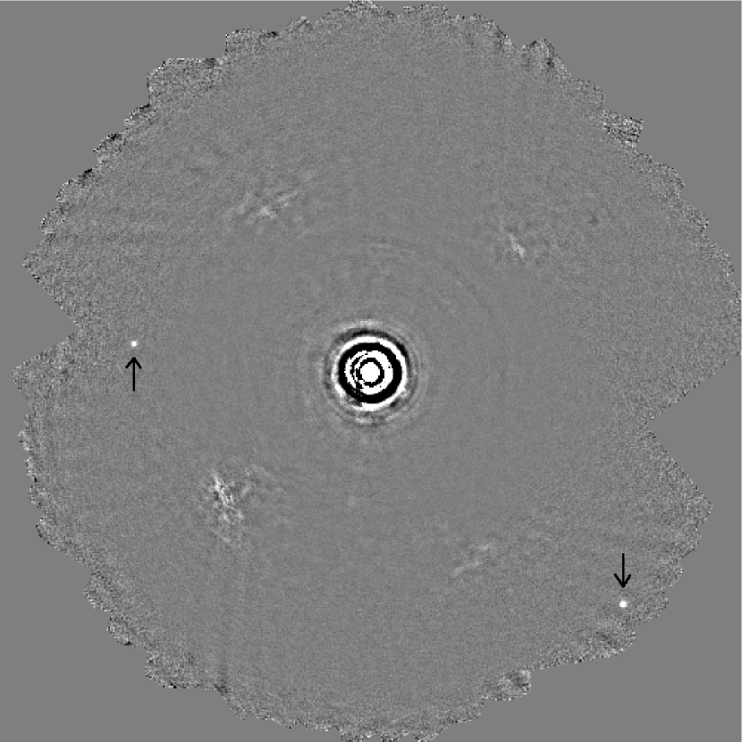
Figure 13: $L^{\prime}$ image of 61 Cyg A, showing two faint background stars. Image is 24.29 arcsec square, contrast stretched the same as the previous figure.

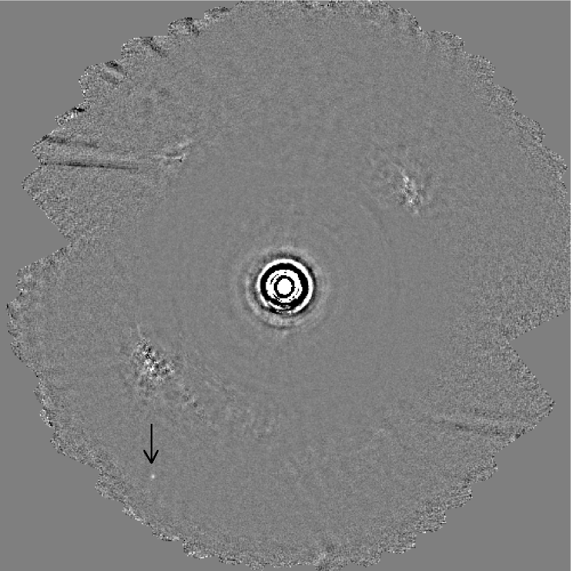
Figure 14: $L^{\prime}$ image of 61 Cyg B, showing a faint background star. Image is 24.29 arcsec square, contrast stretched the same as the previous figure.

We have confirmed that the clean, symmetrical stellar images produced by the MMT AO system at the $L^{\prime}$ and $M$ bands give accurate, consistent center-of-mass centroids even if saturated. This is important for our survey since our pre-stack registration of images is based in most cases on centroids of a saturated primary. If the variation in such centroids is more than about one pixel, faint sources will be substantially blurred in the final stacks, and our point-source sensitivity will be appreciably reduced. In practice, however, we find that faint sources (and bright secondaries in binary systems) do in fact appear sharp in our image stacks. Images we took of Procyon (unpublished) and of 61 Cyg A and B (see Figures 13 and 14) illustrate this in an especially striking manner, because our images of Procyon were more severly saturated than any reported herein, while our 61 Cyg A and B images were among the most saturated in our survey. In all three of these cases, sharp images of faint companions (the orbiting white dwarf in the case of Procyon; background stars in the cases of 61 Cyg A and B) appeared in the final image stacks, which were registered solely based on center-of-mass centroids of the heavily saturated primary. The consistency of such centroids is confirmed to an even tighter tolerence based on our observations of binary survey targets, in which both saturated and unsaturated images were aquired. For example, the total differences between our saturated and unsaturated astrometry at $M$ band for the binary stars GJ 702 and $\xi$ Boo were only 0.0007 arcsec and 0.0039 arcsec, respectively (where differences in separation and position angle have been combined). The same saturated vs. unsaturated differences for our $L^{\prime}$ astrometry of the binary stars $\xi$ Boo, HD 77407, GJ 505, and GJ 166BC were 0.0088 arcsec, 0.0038 arcsec, 0.0026 arcsec, and 0.0015 arcsec, respectively. These values are based on averages of astrometric measurements performed on individual frames prior to stacking. The internal scatter in the astrometry of saturated images was also very low, even though the saturated measurements spanned about an hour of time and tens of degrees of parallactic rotation in each case, giving ample opportunity for any defects in the saturated astrometry to manifest themselves. In all cases tested, center-of-mass centroids of saturated images are self-consistent, and consistent with centroids of unsaturated images, to considerably greater precision than necessary for the purposes of our survey.

We stack our processed images to make a master image for each processing method using a creeping mean combine. This method of image stacking uses a single parameter, the rejection fraction, which we set to 20% for our standard master images. The mean of each given pixel through the image stack is computed, the most deviant value is rejected, and the mean is computed again. This procedure is iterated until the required fraction of data points have been rejected. One of us (S. S.) developed an $N\log(N)$ implementation that greatly improved the speed of our processing pipeline. We chose the creeping mean over the more commonly used median with sigma-clipping because the creeping mean can deliver cleaner final stacks when, as with Clio, the raw images contain bright, slowly-rotating ghosts and diffraction rays. In clean sky away from all ghosts and rays, the median delivers slightly lower rms noise, since it rejects fewer data points.

Our final stacked images contain dark, high-noise regions on either side of each bright star, due to the negative star images from nod subtraction. Since we usually keep a constant nod direction referenced to the telescope, for data sets with significant parallactic rotation the dark regions are spread into arcs and weakened by the creeping mean stack. To further alleviate the dark regions and to enhance the visibility of faint point sources against the bright stellar halo itself, we unsharp mask the final, stacked images. We do this by convolving the image with a Gaussian kernel of $\sigma=5$ pixels, and then subtracting this convolved version from the original image. The full width at half maximum (FWHM) of the Gaussian kernel is 11.8 pixels, as opposed to a FWHM of about 3 pixels for a typical PSF, so the unsharp masking does not strongly reduce the brightness of real point sources. This step marks the end of our image processing pipeline.

The above describes our baseline processing method. We developed six specializations of this method, which we call the ‘b,’ ‘c,’ ‘d,’ ‘e,’ ‘x,’ and ‘y’ processing strategies, while the previously described baseline method itself is called ‘a’. The data from each star in our survey were processed several times, each time using a different one of these specialized methods, and each producing a separate master image. Having multiple master images based on different processing methods is helpful because the different methods enhance sensitivity to planets in different parts of the images, and because the master images from different methods provide a quasi-independent check on the reality of suspected faint sources. We will now describe how these different specialized processing methods function.

In the ‘b’ processing method, we suppress the stellar PSF to increase our sensitivity to faint companions. To do this, we take advantage of the fact that long-lived PSF artifacts in stellar images from AO-equipped telescopes tend to remain fixed with respect to the telescope and/or instrument (Soummer et al., 2007). When observing with the instrument-rotator off, as we do, real sources slowly rotate with respect to artifacts as the telescope tracks. Science images must be digitally rotated before stacking, as described above. However, if a stack of un-rotated frames is made, a clear image of the instrumental PSF is obtained, while any real sources are strongly attenuated by the creeping mean. We subtract a properly registered version of such a PSF image from every science frame prior to final rotation and stacking, a technique called ADI (Marois et al., 2006). In our specific implementation of ADI, we split the image set into a first and second half, and a PSF image is made using a 50% rejection creeping-mean stack of each half. The PSF image from the second half of the data is subtracted from every image in the first half, while the PSF image from the first half of the data is subtracted from the images in the second half. The result is powerful attenuation of the stellar PSF and greatly increased sensitivity to close-in companions. Since parallactic angle changes monotonically with time in all our observing sequences, splitting the data into first and second halves helps prevent real companions from being partially subtracted due to appearing at a residual level in the PSF images. For stars with insufficient parallactic rotation, very close-in companions can still be partially subtracted, but a characteristic dark-bright-dark signature is created which is very noticeable for companions of sufficient brightness. However, in our sensitivity analyses, we have conservatively set the sensitivity of ADI images to zero inside the radius where such ADI self-subtraction first becomes significant.

In the ‘c’ reduction method, an azimuthally smoothed version of the primary PSF is subtracted from the image. The smoothing is done using creeping-mean rejection in a sliding annular arc centered on the primary, with parameters set so that real sources vanish essentially completely from the smoothed PSF and therefore cannot be dimmed in the subtraction. The quality of PSF subtraction achieved is usually substantially inferior to the ‘b’ method, and the ‘c’ method is therefore used relatively seldom. Sometimes it is employed because insufficient parallactic rotation renders the ‘b’ method less useful, or because the ‘c’ image with its different speckle pattern is desired as a quasi-independent check on candidate sources detected in the ‘b’ method image.

In the ‘d’ reduction method, each image is unsharp masked before the stack. The final stacked image is unsharp masked again. While unsharp masking is a linear process, the creeping mean stack is not, so the results are different from simply unsharp-masking twice after the final stack. This is especially significant for bright stars with intense seeing halos. Due to our nod subtraction method, it often happens for such stars that a given x,y pixel location falls on a bright, positive seeing halo for images taken in the first nod position, and on a negative, subtracted seeing halo for images taken in the other nod position: that is, the statistics through the image stack at this pixel location are strongly bimodal. Under such circumstances the creeping mean will settle on either the positive or the negative side of the distribution – and which one it settles on can be different for adjacent pixels. This causes intense ‘bimodality noise’ that is essentially an artifact of the stack. Note that using a median stack instead will not necessarily fix the problem, as there may well be no middle ground between the positive and negative seeing halos. Pre-stack unsharp masking removes the seeing halos and thus resolves the problem of bimodality noise, enormously improving the quality of the final stacked image for bright stars. For fainter stars, the results are more similar to simply unsharp-masking the final image twice. However, the specific noise pattern is substantially changed, which can aid in confirming faint sources: the ‘d’ method image can provide a quasi-independent confirmation for a faint source marginally detected in the baseline ‘a’ image. The ‘e’ data reduction method combines the ‘b’ and ‘d’ methods: ADI is applied, and then the pre-stack unsharp masking is performed.

The ‘x’ data reduction method uses a variant on nod subtraction that avoids the dark negative images. Two master sky images are made, by combining the star-free portions of all images in the first and second halves of the data set. One of these star-free master sky images is then subtracted from each individual science image in lieu of the ordinary nod subtraction. To avoid subtracting real sources, the sky image from the second half of the data set is subtracted from images in the first half, and vice-versa. The usefulness of this processing method varies enormously from one data set to another. If the sky background was very stable, the ‘x’ method final image is almost indistinguishable from that of the baseline ‘a’ method, so that blinking the two gives the impression that the dark nod-subtraction artifacts magically disappear. If the sky background was highly variable, the ‘x’ images are useless due to intense pattern noise. The ‘y’ image reduction method is a combination of the ‘x’ and ‘d’ methods, in which the images are unsharp masked after the subtraction of the master sky image but before the final stack. Figure 2 compares the results of the ‘a’ method (before and after the final unsharp masking step), the ‘d’ method, and the ‘y’ method. The star is HD 96064, a binary system in which the secondary is itself a close binary. A faint additional companion is also detected, but is confirmed based on proper motion and $K_{S}-L^{\prime}$ color to be a background star rather than a substellar companion.

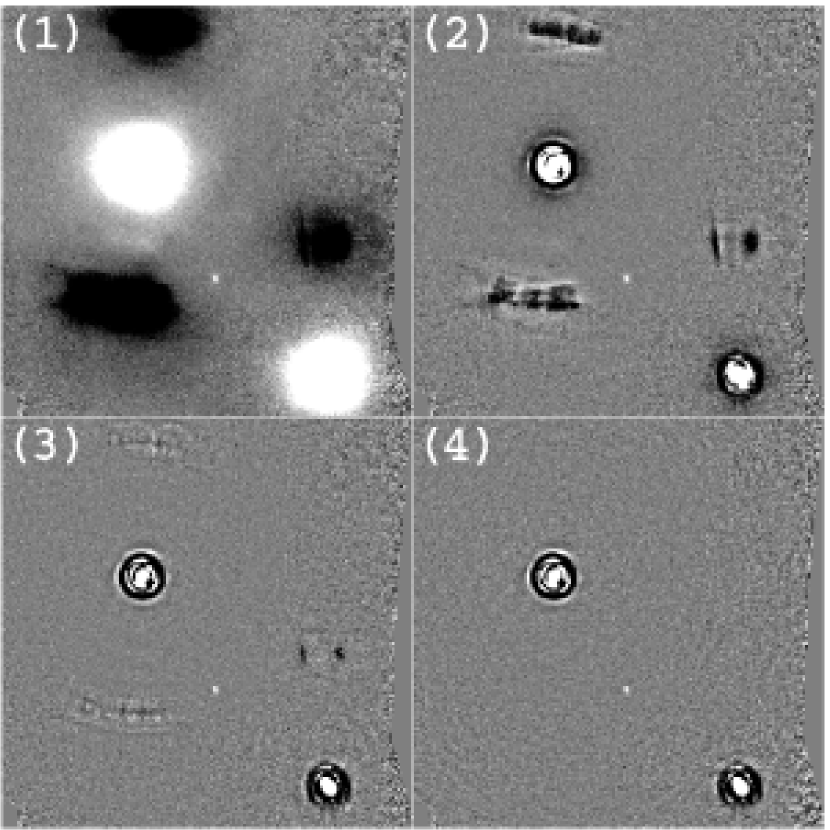
Figure 2: Different processing methods applied to the wide binary star HD 96064. The brightness of the faint source is $L^{\prime}=13.7$, corresponding to a mass of about 20 M_Jup if it were a true companion – however, it is confirmed to be a background star. (1) Result of baseline processing (‘a’ method) before final unsharp mask. (2) The ‘a’ method image after unsharp masking. Dark nod-subtraction artifacts are somewhat reduced but remain prominent. (3) Same data set processed with the ‘d’ method. Nod artifacts are greatly reduced, but still exist as high-noise regions where faint sources could not be detected. (4) Same data set processed with the ‘y’ method. The nod artifacts are eliminated. Field shown in each tile is 17 arcsec square.

Two additional processing methods could be applied to binary stars of near-equal brightness for which both components appeared on each Clio frame. A scaled version of the PSF of each star could be used to subtract the other, on a frame-by-frame basis, prior to the final stack. The resulting PSF subtraction was substantially better than ADI. We labeled this reduction method ‘f.’ A version that also included pre-stack unsharp masking was called ‘g’. Figure 3 illustrates our different PSF subtraction methods, both ADI and binary star subtraction, as applied to the binary star GJ 896, which was also shown in Figure 1.

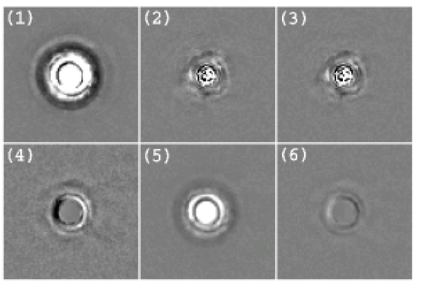
Figure 3: (1) Baseline ‘a’ method final image of GJ 896A. (2) Same data set processed with ADI (‘b’ method). (3) Same data set processed with ADI and pre-stack unsharp masking (‘e’ method). (4) Same data set processed with binary star subtraction. Background noise is increased because the secondary had to be scaled up to match the brightness of the primary. (5) Same data set, but now showing the ‘a’ method image of the secondary, rather than the primary. (6) Same data set, again showing the secondary, but now processed with binary star subtraction. The background is very clean since the primary was scaled down to subtract away the secondary. Field shown in each tile is 3.9 arcsec square.

We applied the ‘a,’ ‘b,’ ‘d,’ and ‘e’ processing methods to almost all of our stellar data sets, except a very few for which there was insufficient parallactic rotation to use the ADI methods without subtracting real sources. In many instances we also applied the ‘x’ and ‘y’ methods. We applied the ‘f’ and ‘g’ methods to every binary star where they would work.

The methods involving pre-stack unsharp masking (‘d,’ ‘e,’ ‘y,’ and ‘g’) always gave cleaner images, but we used the other methods as well because pre-stack masking slightly dimmed point sources (by about 3-10%, depending on the AO-corrected FWHM), and there was a slight chance this could cause a discovery to be missed. Our pattern-noise correction method also dimmed faint point sources by about 15-18%, based on tests. Near the end of our processing, one of us (M. K.) developed a superior pattern-noise correction that caused zero dimming, and we also developed a type of unsharp masking that produced zero dimming to within the measurement error of our tests. Only the stars $\epsilon$ Eri ($L^{\prime}$ and $M$ band), GJ 684 A, GJ 684 B, GJ 702 A ($M$ band only), GJ 702 B ($M$ band only), 61 Cyg B ($M$ band only), GJ 860 A, and GJ 860 B were processed using these improvements. For these stars, only the ‘d,’ ‘e,’ ‘y,’ and, where applicable, the ‘g’ processing methods were used, since the downside of pre-stack unsharp masking had been eliminated.

4 Sensitivity Analysis

4.1 Sensitivity Estimators

Our survey arrived at a null result: no planets were detected. Our science results, like those of previous surveys (Masciadri et al., 2005; Kasper et al., 2007; Biller et al., 2007; Lafrenière et al., 2007; Chauvin et al., 2010), therefore take the form of upper limits on the abundance of extrasolar planets. The accuracy of such an upper limit depends entirely on having a good metric for the sensitivity of the survey observations.

A sensitivity estimator must translate some measurable statistic of an image into a realistic point-source detection limit. A procedure which has often been used (see for example Biller et al. (2007) and Chauvin et al. (2010)) involves calculating the single-pixel RMS standard deviation ($\sigma_{pix}$) in different regions on an image, and adopting a factor (often taken to be 5.0) by which the peak of a point-source image must exceed this $\sigma_{pix}$ to be cleanly detected. All that remains is to map the $5\sigma_{pix}$ PSF peak to a magnitude (or $\Delta$-mag), and assign this as the sensitivity in the image region under consideration. Biller et al. (2007) and Kasper et al. (2007), among others, have discussed possible choices for the size and shape of the regions over which $\sigma_{pix}$ is calculated, with the objective of obtaining smooth and accurate plots of point-source sensitivity vs. separation from the star.

While the method above produces excellent results when correctly applied, we sought to adopt a slightly more sophisticated approach. One reason for this is that calculating sensitivity based on comparing the single-pixel RMS to the peak of the PSF does not take into account the FWHM of the PSF. If the PSF is several pixels wide, detection need not depend on the peak height alone: pixels other than the central peak contain additional flux that can in principle be used to detect the point source at a lower peak flux than would be possible for a narrower PSF. We have explored three possible sensitivity estimation methods that attempt to consider all the flux contained in the image of a point source, rather than only the peak of the PSF. The first solution we considered was calculating $\sigma_{pix}$ just as for the previous method, and then translating this to a detection limit using simple $\sqrt{n}$ statistics:

$$\sigma_{PSF}=\sigma_{pix}\sqrt{\pi r^{2}}=\sigma_{pix}r\sqrt{\pi}.$$ (1)

Where $\sigma_{PSF}$ is the PSF-scale noise in the image, $\sigma_{pix}$ is the single-pixel RMS as before, and $r$ is the radius of the image of a point source (i.e. about half the FWHM of the PSF). Since not all the flux of a real point source will fall within the aperture of radius $r$, an aperture correction must be applied as a final step. Then, for example, the 5$\sigma$ point-source sensitivity will be 5 $\sigma_{PSF}$ times the aperture correction. This sensitivity limit would represent an actual integrated flux, which could be converted directly to magnitudes using a photometric calibration. We will call this sensitivity estimation technique ‘Method 1’.

The simple $\sqrt{n}$ statistics used in Method 1 assume that the brightness of each pixel is a random variable independent of its neighboring pixels: that is, that the noise is spatially uncorrelated. This assumption is violated for speckle residuals close to a star, and for a host of other stellar artifacts that are present in AO images (ghosts, diffraction rays, etc.). We have confirmed by careful tests that in the presence of speckle noise, Method 1 overestimates the true point-source sensitivity by up to 0.9 magnitudes. This applies to a good implementation of the method in which $\sigma_{pix}$ is calculated over image regions spanning many PSF sizes. When the statistics region used is too small, the sensitivity will be overestimated even more.

The problem with Method 1 is that clumps of correlated bright or dark pixels introduce more PSF-scale noise into the image than can be predicted from the single-pixel RMS. Lafrenière et al. (2007) solved this problem by convolving their image with a circular disk of radius $r$, effectively summing up the brightness within many small circular apertures at this radius, one aperture centered on each pixel throughout the image. Then $\sigma_{PSF}$ will simply equal the RMS variation of the aperture sums (that is, of the convolved image). This is sensitivity estimation by aperture photometry of the noise background. As with previously discussed methods, it is important to calculate the statistic over an image region large enough to contain many PSFs. In our implementation, the region over which the statistic $\sigma_{PSF}$ is calculated is either a disk of 8 pixel radius, or, close to the star, an annular arc one pixel wide and 45 pixels long, at constant radius from the star. For simplicity, we will sometimes refer to this Lafrenière et al. (2007) method as ‘Method 2’. As with Method 1, an aperture correction must be applied as a final step.

Method 3 has already been described in Heinze et al. (2008). It is analagous to Method 2, but rather than performing aperture photometry centered on every pixel of the image, one performs PSF-fitting photometry. If the PSF has been properly normalized, no aperture correction is necessary for this method. We used PSF images from the short, unsaturated exposures described in Section 3.2.

In tests using our own real data, we find that the Lafrenière et al. (2007) method and Method 3 agree to within reasonable uncertainty everywhere, while Method 1 agrees with the other two only in regions of very clean sky. Method 1 overestimates the sensitivity by about 0.2 magnitudes in the presence even of very faint ghost residuals, and by about 0.9 magnitudes in the strong residual speckle noise close to the star. Herein, as in Heinze et al. (2008), we have used Method 3 for our final sensitivity maps. It seemed slightly more conservative close to the star than Method 2, though, again, our tests showed no significant difference between Method 3 and the method of Lafrenière et al. (2007). Far from the primary star, the region we use for calculating the sensitivity statistic is a disk of radius 8 pixels (0.39 arcsec, or about 3 $\lambda/D$): that is, large enough to span many PSF-sizes, but small enough to sample the local noise properties. Close to the star (that is, within 60 pixels or 2.9 arcsec), we use instead an arc 45 pixels (2.2 arcsec) long and 1 pixel wide, at a fixed radius from the star. These disks or arcs are centered in turn on every pixel of each image, with the calculated statistics forming a sensitivity map.

4.2 Sensitivity Obtained

After making a sensitivity map from the stacked image produced by each processing method applied to the data from a given star, we apply a slight smoothing to the different maps, and then combine them into a single master sensitivity map. They are combined such that the master sensitivity image shows at each location the best sensitivity obtained at that location by any processing method that was applied. We quote 10$\sigma$ sensitivities: that is, the point source sensitivity is ten times the $\sigma_{PSF}$ statistic from Method 3. 10$\sigma$ is chosen as a nominal detection threshold because we have over 95% completeness for 10$\sigma$ sources, with considerably less for 5 or 7$\sigma$ (see Section 4.4).

Our background-limited 10$\sigma$ sensitivity for one-hour exposures under fair conditions is typically $L^{\prime}=16.0$, or $M=13.0$. Since we can detect some sources down to 5$\sigma$ significance, this corresponds to some chance of finding objects as faint as $L^{\prime}=16.75$ or $M=13.75$. For exposures longer than an hour or under very good conditions, our background limited 10$\sigma$ sensitivity ranged as high as $L^{\prime}=16.5$ or $M=13.3$. Our median 10$\sigma$ sensitivities close to the stars were about $\Delta$mag$=6.0$ at 0.5 arcsec and $\Delta$mag$=8.7$ at 1.0 arcsec, though the values could range as high as 7.2 and 9.8, respectively. The $\Delta$mag values obtained by shorter wavelength AO observations (e.g. Biller et al. (2007) and Lafrenière et al. (2007)) are much better due to the smaller diffraction disk at these wavelengths, but this effect is substantially compensated by the more favorable planet/star flux ratios at the $L^{\prime}$ and $M$ bands. See Heinze et al. (2008) for a detailed comparison of the efficacies of different wavelengths for planet detection in the specific cases of Vega and $\epsilon$ Eri.

Figures 4, 5, and 6 give example sensitivity contour maps for our $L^{\prime}$ observations of GJ 896 and GJ 117, and our $M$ band observations of 61 Cyg B, respectively, with 10$\sigma$ sensitivities given in apparent magnitudes. Figures of this type for all the stars observed in our survey can be downloaded from http://www.hopewriter.com/Astronomyfiles/Data/SurveyPaper/.

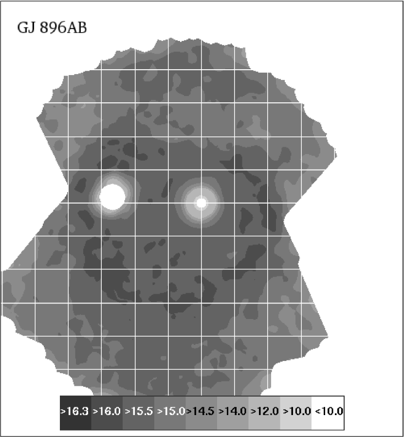
Figure 4: Final sensitivity contour map for the binary star GJ 896 AB. 10$\sigma$ sensitivities from our Method 3 estimator are presented, converted to apparent $L^{\prime}$ magnitudes. The grid squares superposed for astrometric reference are 2$\times$2 arcsec. The darkest contour from the colorbar is not present as the 10$\sigma$ sensitivity in this data set never exceeded $L^{\prime}=16.3$.

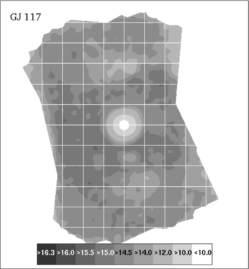
Figure 5: Final sensitivity contour map for the star GJ 117. 10$\sigma$ sensitivities from our Method 3 estimator are presented, converted to apparent $L^{\prime}$ magnitudes. The grid squares superposed for astrometric reference are 2$\times$2 arcsec, with the primary star in the figure’s center. The darkest two contours from the colorbar are not present as the 10$\sigma$ sensitivity in this data set never exceeded $L^{\prime}=16.0$.

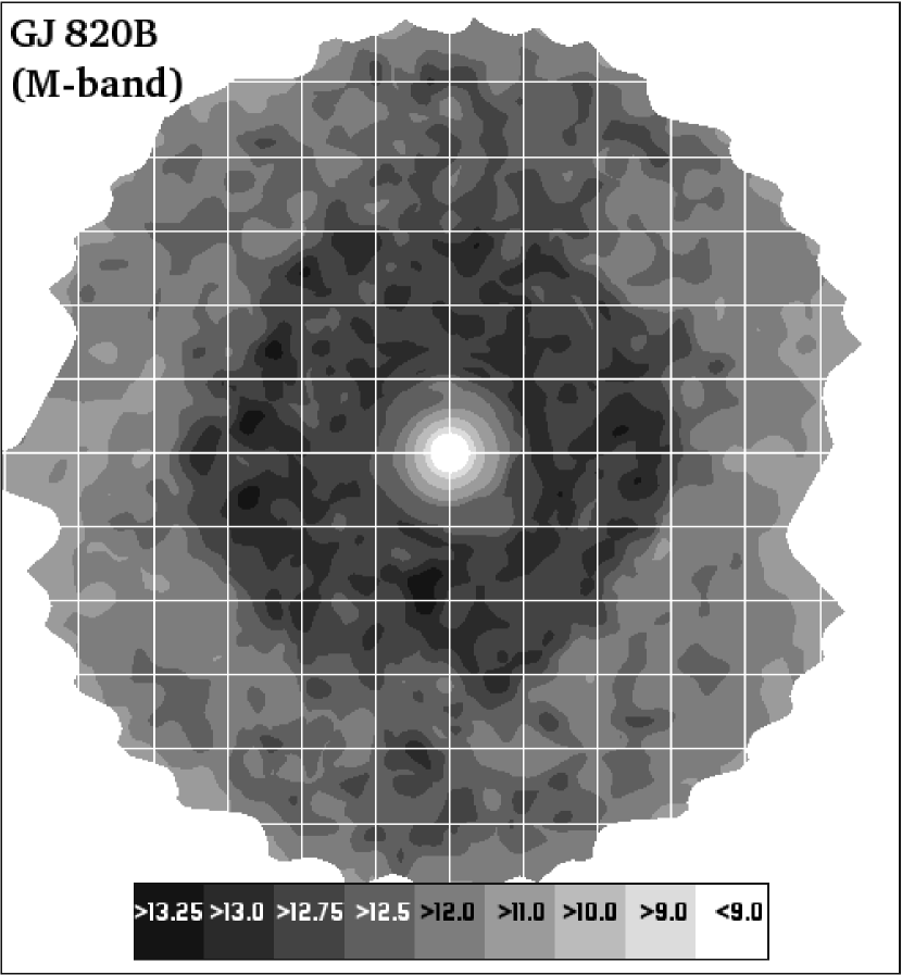
Figure 6: Final sensitivity contour map for our $M$ band observations of the star 61 Cyg B (GJ 820 B). 10$\sigma$ sensitivities from our Method 3 estimator are presented, converted to apparent $M$ band magnitudes. The grid squares superposed for astrometric reference are 2$\times$2 arcsec.

For use in the Monte Carlo simulations described in Heinze et al. (2010), we have converted our sensitivity maps into plots of sensitivity vs. projected radius from each star. As can be seen from Figures 4 through 6, however, our sensitivity varied widely with position angle around the star. To quantify this, we calculated ten different sensitivity values at each radius, giving the percentiles in sensitivity from 0th to 90th percentile in 10% increments. Thus, e.g., the 0th percentile at 2 arcsec is the very worst sensitivity obtained anywhere on the 2 arcsec-radius ring surrounding the star, while the 50th percentile gives the median sensitivity at that radius. In Figures 7 and 8, we give example plots for GJ 896 A, GJ 117, 61 Cyg B ($M$ band), and $\epsilon$ Eri, with the sensitivities converted to minimum detectable planet mass in M_Jup using models from Burrows et al. (2003), plotted against projected separation in AU. Plots of this type for all the stars in our survey, as well as the tabular data from which they were constructed, can be downloaded from http://www.hopewriter.com/Astronomyfiles/Data/SurveyPaper/.

Figure 7: Minimum detectable planet mass vs. projected separation in AU for GJ 896 A (left) and GJ 117 (right). 10$\sigma$ detection limits from Method 3 are shown, converted to planet mass using models from Burrows et al. (2003). Planetary orbits around GJ 896 A would be destabilized beyond about 12 AU by the companion star GJ 896 B. In order from bottom to top, the curves give the 90th, 80th, 70th, 60th, 50th, 40th, 30th, 20th, 10th, and 0th percentile sensitivity at each radius.

Figure 8: Minimum detectable planet mass vs. projected separation in AU for 61 Cyg B ($M$ band data; left), and $\epsilon$ Eri (right). 10$\sigma$ detection limits from Method 3 are shown, converted to planet mass using models from Burrows et al. (2003). In order from bottom to top, the curves give the 90th, 80th, 70th, 60th, 50th, 40th, 30th, 20th, 10th, and 0th percentile sensitivity at each radius.

4.3 Source Detection

While our final sensitivity maps are constructed using only Method 3, as described above, we use both Methods 2 and 3 for automated source detection. The use of both methods increases our likelihood of noticing faint sources at the limit of detectability. To search an image for sources using either method, we query each pixel in turn to see if a source is present at that location. To make this query, we first calculate the sensitivity statistic (Method 2 or Method 3) over either a disk or an arc, just as described in Section 4.1, except that a PSF-sized region around the pixel being considered is not included, so that if a real source is present, it will not bias the sensitivity estimator. Finally, either aperture photometry (Method 2) or PSF-fitting (Method 3) is applied at the location of the pixel itself, measuring the brightness of any source that may be present there. If the resulting brightness is greater than the sensitivity statistic by a specified threshold factor (i.e., 5 for a 5$\sigma$ detection), a preliminary detection is reported.

We would like to set the threshold as low as possible without getting an unmanageable number of spurious detections. To this end, we divided each data set into the first half of the images and the second half, and created a stacked image from each half. To be reported by our automated detection code, a source had to appear at $4.5\sigma$ significance in the full stack, and at $3\sigma$ significance on each half-stack, at a location consistent to within 2 pixels. This eliminated residual ghosts and other artifacts, which would appear in different locations on the two halves of the data due to parallactic rotation. Typically 10-20 spurious automated detections were nonetheless reported around each star.

A real source could also be missed by the automatic algorithm but noticed manually. For example, due to parallactic rotation, a location might have valid data only for the first half of the data sequence, rendering an automated detection of a real source there impossible. Every automated detection, as well as candidate sources noticed only by eye, was carefully examined manually. Criteria applied included correct FWHM and symmetry, consistency in position and brightness from one half-stack to the other, and inability to be explained away as an artifact of ghosts, diffraction rays, etc. If necessary, data stacks were split into quarters or even finer divisions to verify sources where only a fraction of the images provided useful data. These manual investigations were very labor-intensive, especially since the master images and half-stacks from several different processing methods (see Section 3.3) had to be examined for each star. Every source that passed this final manual analysis was found to correspond to a real astronomical object. There were no false positives.

4.4 Blind Sensitivity Tests

The final demonstration of the validity of a sensitivity estimator is a blind sensitivity test, in which fake planets are inserted into the raw data and then recovered by an experimenter (or automated process) without a-priori knowledge of their positions or their number. Such a blind test is the surest way to evaluate any sensitivity estimator and establish the relationship between nominal significance (i.e. 3$\sigma$, 5$\sigma$, etc.) and the true completeness level of the survey. This should be standard procedure for all planet imaging surveys.

We inserted simulated planets at random locations in the raw data for selected stars. The flux of each simulated planet was scaled to 5, 7, or 10$\sigma$ significance based on the master sensitivity map (see Section 4.2) for that star. The PSFs for the planets were taken from the short exposure, unsaturated images of the parent star, mentioned above in Section 3.2. The raw data with fake planets inserted was then processed exactly as for the real, unmodified science data for that star, and planets were sought in the fully processed images by the same combination of manual and automatic methods used for the real images.

The final result of each test was that every inserted planet was classified as ‘Confirmed’, ‘Noticed’, or ‘Unnoticed’. ‘Confirmed’ means the source was confidently detected, with no significant doubt of its being a real object. ‘Noticed’ means the source was flagged by our automatic detection algorithm, or noticed manually as a possible real object, but could not be confirmed beyond reasonable doubt. Many spurious sources are ‘Noticed’ whereas the false-positive rate for ‘Confirmed’ detections is extremely low, with none for any of the data sets discussed here. ‘Unnoticed’ means a fake planet was not automatically flagged or noticed manually.

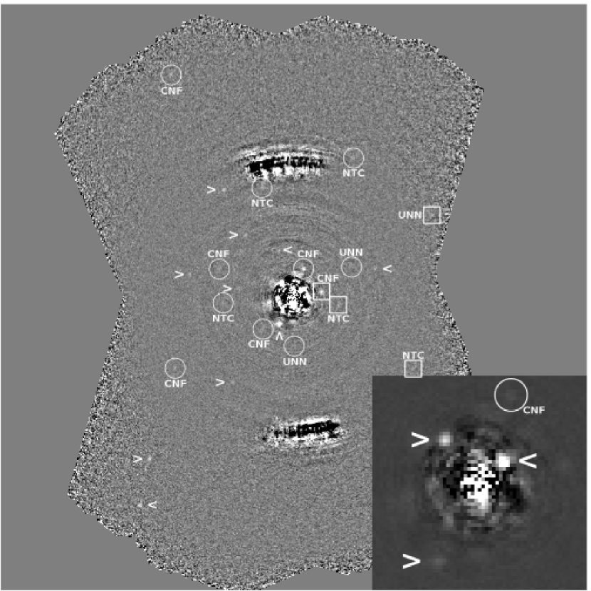
Figure 9: Fully processed ‘e’ method master image from the blind sensitivity test on HD 29391. In this data set there are 12 planets of 10$\sigma$ significance (indicated by arrows), 10 at 7$\sigma$ (circled), and 5 at 5$\sigma$ (boxed). One 5$\sigma$ planet is hidden by the inset. Each planet was either confirmed (CNF), noticed (NTC), or unnoticed (UNN) in the blind test. All 10$\sigma$ planets were confirmed. The inset, 3 arcsec square, shows the inner part of the image magnified 3$\times$ and with display range increased 10$\times$ relative to the main image. The main image is 24 arcsec square. Two planets are marked in both the main image and the inset.

Tables 5 through 9 give the results of these simulations, showing how the detectable planet masses vary with the distance and age of the stars, and with data quality. Note that simulated planets with masses ranging down to 3 M_Jup and below were confirmed, the lowest mass planet confirmed being one of 2.36 M_Jup in the GJ 117 simulation. Figure 9 shows an image from our blind sensitivity test on HD 29391, with the simulated planets marked. The random positions of the planets, unknown by the experimenter attempting to detect the them, are an important aspect of our tests.

Table 5: GJ 450 fake planet experiment.

Sep		Mass	Detection
(arcsec)	$L^{\prime}$ Mag	(MJup)	Significance	Status
0.51	12.53	$>$20	10.00$\sigma$	Confirmed
0.56	13.32	$>$20	10.00$\sigma$	Confirmed
0.95	15.35	11.26	10.00$\sigma$	Confirmed
1.14	15.60	10.54	10.00$\sigma$	Confirmed
1.27	15.96	9.51	10.00$\sigma$	Confirmed
1.58	16.06	9.21	10.00$\sigma$	Confirmed
1.90	16.51	7.93	10.00$\sigma$	Confirmed
2.50	16.59	7.73	10.00$\sigma$	Confirmed
2.69	16.57	7.78	10.00$\sigma$	Confirmed
2.91	16.38	8.29	10.00$\sigma$	Confirmed
2.98	16.60	7.70	10.00$\sigma$	Confirmed
3.71	16.51	7.93	10.00$\sigma$	Confirmed
3.90	16.59	7.73	10.00$\sigma$	Confirmed
3.93	16.62	7.65	10.00$\sigma$	Confirmed
5.02	16.49	7.98	10.00$\sigma$	Confirmed
6.52	16.43	8.15	10.00$\sigma$	Confirmed
6.53	16.27	8.61	10.00$\sigma$	Confirmed

Note. — All of the input planets were confirmed. Planet magnitude to mass conversion carried out by interpolation based on theoretical spectra from Burrows et al. (2003), using our adopted distance and age for this star (8.1 pc, 1.0 Gyr).

Table 6: HD 29391 fake planet experiment.

Sep		Mass	Detection
(arcsec)	$L^{\prime}$ Band Mag	(MJup)	Significance	Status
0.42	11.59	$>$20	10.00$\sigma$	Confirmed
0.76	12.56	16.85	10.00$\sigma$	Confirmed
1.23	15.35	4.97	10.00$\sigma$	Confirmed
2.06	15.90	3.92	10.00$\sigma$	Confirmed
2.27	16.10	3.63	10.00$\sigma$	Confirmed
3.26	14.58	6.95	10.00$\sigma$	Confirmed
3.60	15.77	4.15	10.00$\sigma$	Confirmed
4.29	15.48	4.72	10.00$\sigma$	Confirmed
4.41	16.22	3.46	10.00$\sigma$	Confirmed
5.31	16.21	3.47	10.00$\sigma$	Confirmed
8.92	16.15	3.56	10.00$\sigma$	Confirmed
10.69	16.15	3.56	10.00$\sigma$	Confirmed
1.25	15.17	5.40	7.00$\sigma$	Confirmed
1.86	16.32	3.31	7.00$\sigma$	Confirmed
2.00	16.47	3.09	7.00$\sigma$	Unnoticed
2.69	16.54	2.99	7.00$\sigma$	Unnoticed
2.92	16.61	2.93	7.00$\sigma$	Noticed
3.29	16.47	3.09	7.00$\sigma$	Confirmed
4.69	15.83	4.03	7.00$\sigma$	Noticed
5.72	16.38	3.22	7.00$\sigma$	Confirmed
6.28	15.97	3.82	7.00$\sigma$	Noticed
10.53	15.94	3.86	7.00$\sigma$	Confirmed
1.19	15.39	4.89	5.00$\sigma$	Confirmed
1.93	16.77	2.78	5.00$\sigma$	Noticed
5.76	16.57	2.97	5.00$\sigma$	Noticed
6.68	16.25	3.41	5.00$\sigma$	Unnoticed
7.70	16.18	3.51	5.00$\sigma$	Unnoticed

Note. — Planets confirmed: 12/12 at 10$\sigma$; 5/10 at 7$\sigma$; 1/5 at 5$\sigma$. Planets noticed: 12/12 at 10$\sigma$; 8/10 at 7$\sigma$; 3/5 at 5$\sigma$. Planet magnitude to mass conversion carried out by interpolation based on theoretical spectra from Burrows et al. (2003), using our adopted distance and age for this star (14.71 pc, 0.1 Gyr).

Table 7: GJ 117 fake planet experiment.

Sep		Mass	Detection
(arcsec)	$L^{\prime}$ Band Mag	(MJup)	Significance	Status
0.67	10.41	$>$20.0	10.00$\sigma$	Confirmed
0.94	11.54	15.42	10.00$\sigma$	Confirmed
1.10	12.05	12.21	10.00$\sigma$	Confirmed
2.11	15.01	3.42	10.00$\sigma$	Confirmed
2.17	14.78	3.75	10.00$\sigma$	Confirmed
3.31	14.93	3.53	10.00$\sigma$	Confirmed
3.77	15.20	3.14	10.00$\sigma$	Confirmed
6.40	14.72	3.84	10.00$\sigma$	Confirmed
6.42	15.26	3.05	10.00$\sigma$	Confirmed
8.60	15.06	3.35	10.00$\sigma$	Confirmed
9.88	14.56	4.09	10.00$\sigma$	Confirmed
1.14	12.54	9.77	7.00$\sigma$	Confirmed
3.08	15.44	2.87	7.00$\sigma$	Noticed
5.06	15.35	2.96	7.00$\sigma$	Confirmed
6.37	14.67	3.91	7.00$\sigma$	Noticed
7.04	14.66	3.93	7.00$\sigma$	Noticed
7.88	15.27	3.05	7.00$\sigma$	Noticed
1.04	12.31	10.83	5.00$\sigma$	Confirmed
1.75	15.12	3.26	5.00$\sigma$	Unnoticed
2.89	15.96	2.40	5.00$\sigma$	Unnoticed
3.30	16.16	2.21	5.00$\sigma$	Unnoticed
5.08	16.00	2.36	5.00$\sigma$	Confirmed
7.80	15.32	2.98	5.00$\sigma$	Noticed
8.03	15.65	2.68	5.00$\sigma$	Unnoticed
10.21	15.30	3.00	5.00$\sigma$	Noticed

Note. — Planets confirmed: 11/11 at 10$\sigma$; 2/6 at 7$\sigma$; 2/8 at 5$\sigma$. Planets noticed: 11/11 at 10$\sigma$; 6/6 at 7$\sigma$; 4/8 at 5$\sigma$. Planet magnitude to mass conversion carried out by interpolation based on theoretical spectra from Burrows et al. (2003), using our adopted distance and age for this star (8.31 pc, 0.1 Gyr). Note that a fake planet with a mass of only 2.36 M_Jup was confirmed.

Table 8: GJ 355 fake planet experiment.

Sep		Mass	Detection
(arcsec)	$L^{\prime}$ Band Mag	(MJup)	Significance	Status
0.37	9.46	$>$20.0	10.00$\sigma$	Confirmed
0.43	9.66	$>$20.0	10.00$\sigma$	Confirmed
0.94	13.72	13.10	10.00$\sigma$	Confirmed
1.67	15.61	5.74	10.00$\sigma$	Confirmed
1.74	15.66	5.63	10.00$\sigma$	Confirmed
1.85	15.74	5.43	10.00$\sigma$	Confirmed
2.05	15.63	5.70	10.00$\sigma$	Confirmed
2.37	15.87	5.11	10.00$\sigma$	Noticed
3.08	15.60	5.78	10.00$\sigma$	Confirmed
3.30	15.92	5.00	10.00$\sigma$	Confirmed
3.44	15.73	5.46	10.00$\sigma$	Confirmed
4.26	16.02	4.80	10.00$\sigma$	Confirmed
5.55	15.87	5.12	10.00$\sigma$	Confirmed
8.09	15.55	5.89	10.00$\sigma$	Confirmed
8.70	15.34	6.46	10.00$\sigma$	Confirmed
1.57	15.95	4.93	7.00$\sigma$	Noticed
2.83	16.24	4.37	7.00$\sigma$	Noticed
3.68	16.04	4.77	7.00$\sigma$	Confirmed
4.34	16.01	4.82	7.00$\sigma$	Confirmed
4.68	16.33	4.19	7.00$\sigma$	Noticed
6.99	15.95	4.94	7.00$\sigma$	Confirmed
1.92	16.58	3.78	5.00$\sigma$	Unnoticed
3.24	16.52	3.87	5.00$\sigma$	Unnoticed
5.61	15.93	4.99	5.00$\sigma$	Noticed
5.99	15.86	5.16	5.00$\sigma$	Noticed
7.17	15.94	4.97	5.00$\sigma$	Noticed
10.07	16.31	4.23	5.00$\sigma$	Confirmed

Note. — Planets confirmed: 14/15 at 10$\sigma$; 3/6 at 7$\sigma$; 1/6 at 5$\sigma$. Planets noticed: 15/15 at 10$\sigma$; 6/6 at 7$\sigma$; 4/6 at 5$\sigma$. Planet magnitude to mass conversion carried out by interpolation based on theoretical spectra from Burrows et al. (2003), using our adopted distance and age for this star (19.23 pc, 0.1 Gyr).

Table 9: BD+48 3686 fake planet experiment.

Sep		Mass	Detection
(arcsec)	$L^{\prime}$ Band Mag	(MJup)	Significance	Status
0.23	8.03	$>$20.0	10.00$\sigma$	Confirmed
0.97	14.65	13.89	10.00$\sigma$	Noticed
1.33	15.19	10.47	10.00$\sigma$	Confirmed
2.05	15.51	9.05	10.00$\sigma$	Confirmed
4.33	15.57	8.85	10.00$\sigma$	Confirmed
5.08	15.70	8.41	10.00$\sigma$	Confirmed
6.13	15.52	9.04	10.00$\sigma$	Confirmed
6.34	14.70	13.53	10.00$\sigma$	Confirmed
8.41	15.38	9.60	10.00$\sigma$	Confirmed
9.73	15.46	9.26	10.00$\sigma$	Confirmed
1.46	15.62	8.67	7.00$\sigma$	Confirmed
2.55	15.86	7.87	7.00$\sigma$	Noticed
3.76	16.15	7.05	7.00$\sigma$	Unnoticed
5.25	15.72	8.32	7.00$\sigma$	Confirmed
5.73	15.66	8.53	7.00$\sigma$	Unnoticed
10.43	15.41	9.50	7.00$\sigma$	Confirmed
1.08	15.63	8.66	5.00$\sigma$	Noticed
3.04	16.39	6.45	5.00$\sigma$	Unnoticed
3.34	16.29	6.70	5.00$\sigma$	Unnoticed
5.69	16.40	6.42	5.00$\sigma$	Noticed
9.19	16.17	7.00	5.00$\sigma$	Unnoticed
10.22	15.97	7.56	5.00$\sigma$	Noticed

Note. — Planets confirmed: 9/10 at 10$\sigma$; 3/6 at 7$\sigma$; 0/6 at 5$\sigma$. Planets noticed: 10/10 at 10$\sigma$; 4/6 at 7$\sigma$; 3/6 at 5$\sigma$. Planet magnitude to mass conversion carried out by interpolation based on theoretical spectra from Burrows et al. (2003), using our adopted distance and age for this star (23.6 pc, 0.15 Gyr).

The total statistics from all 5 blind tests are that 63 of 65 planets were confirmed at 10$\sigma$, 13 of 28 at 7$\sigma$, and 4 of 25 at 5$\sigma$. In percentages we have 97% completeness at 10$\sigma$, 46% completeness at 7$\sigma$, and 16% completeness at 5$\sigma$.

Note the very low completeness at 5$\sigma$, which many past surveys have taken as a realistic detection limit. Though sensitivity estimators (and therefore the exact meaning of 5$\sigma$) differ, ours was quite conservative. The low completeness we find at 5$\sigma$ should serve as a warning to future workers in this field, and an encouragement to establish a definitive significance-completeness relation through blind sensitivity tests as we have done. Many more planets were noticed than were confirmed: for noticed planets, the rates are 100% at 10$\sigma$, 86% at 7$\sigma$, and 56% at 5$\sigma$. However, very many false positives were also noticed, so sources that are merely noticed but not confirmed do not represent usable detections. No false positives were confirmed in any of our blind tests.

There are several reasons for our low completeness rate at $5\sigma$. First, some flux is lost from faint sources in our processing, as described above, so that sources input at 5$\sigma$ significance are reduced to a real significance of typically 4$\sigma$ in the final image. Second, since our images contain speckles, ghosts, diffraction rays, and pattern noise, the noise is not gaussian but rather has a long tail toward improbable, bright events – a normal circumstance in AO images that has been carefully described by Fitzgerald & Graham (2006) and Marois et al. (2008). Third, the area of each final image is over $10^{5}$ times the size of a PSF, so the distribution of possible spurious planet images arising from noise is sampled at least $10^{5}$ times for each final image in our survey. Followup observations of suspected sources are costly in terms of telescope time, so a detection strategy with a low false-positive rate is important.

While background noise originating from photon statistics in astronomical images is gaussian, speckle noise in AO-corrected images close to bright stars has been shown to follow a longer tailed, approximately rician distribution (Marois et al., 2008; Fitzgerald & Graham, 2006). In fact, Marois et al. (2008) have shown that to obtain an acceptably low false positive rate, detection thresholds must be set as high as $12\sigma$ in the presence of severe speckle noise. They assume a detection strategy based on the single-pixel RMS standard deviation (e.g. Biller et al. (2007); Chauvin et al. (2010)) rather than sensitivity estimation methods like ours or that of Lafrenière et al. (2007). Even so, given their findings it may seem surprising not that we had low completeness at $5\sigma$, but that we were able to detect some $5\sigma$ sources while also maintaining a very low false-positive rate.

Part of the explanation for this is the speckle-supression produced by ADI: Marois et al. (2008) found that ADI could be so powerful that it nearly restored gaussian statistics to an image, allowing the viable detection threshold to drop from $12\sigma$ to lower than $6\sigma$. Our implementation of ADI may not be as effective as that of Marois et al. (2008), but it did substantially improve our image statistics. This is demonstrated by the fact that our blind sensitivity tests did not show any clear bias against detection of low-significance planets close to the star. However, some of our ability to confirm low-significance planets is simply due to our painstaking detection strategy. Noise-bursts at 10 or 12 $\sigma$ may occur in the speckle-dominated regions of AO images, but splitting the data in half, examining master images created using different processing methods, and other time-intensive analyses can powerfully sort out the real from the unreal – even, in some cases, when the spurious sources are substantially brighter.

Accurate estimation of the sensitivity of AO images is a complex task, worthy, perhaps, of more attention than has been paid it in the AO planet-search literature up to this point. Between this work, Lafrenière et al. (2007), Biller et al. (2007) and Kasper et al. (2007), and others, several different sensitivity estimators have been used, which may produce substantially different results. Statistical noise distributions can vary widely even on a single image (Marois et al., 2008), and certainly exhibit further variability from instrument to instrument and telescope to telescope. A blind sensitivity test such as we have carried out is an excellent way to determine the true sensitivity of a set of observations. Completeness vs. significance relations established by such blind sensitivity tests may represent the only real option for ‘apples-to-apples’ comparisons of the sensitivity obtained with different instruments on different telescopes – and such comparisons may be quite important for selecting optimal observing strategies as we move forward to the next generation of surveys to detect extrasolar planets.

5 Detections of Faint Real Objects

5.1 Overview of Detected Companions

In all, thirteen faint sources were confirmed as real. Table 10 presents our astrometry and photometry for each detected companion.

Table 10: Confirmed Sources in Our Survey

Star	Det.	$L^{\prime}$	Sep		Date
Name	Sig.	Mag	(arcsec)	PA	(yyyy/mm/dd)
GJ 354.1A	4.93$\sigma$	$16.48\pm 0.20$	4.93	$187.3^{\circ}$	2006/04/12
GJ 564	175.68$\sigma$	$10.80\pm 0.20$	2.60	$103.0^{\circ}$	2006/04/13
GJ 3876	246.38$\sigma$	$10.88\pm 0.20$	1.85	$118.6^{\circ}$	2006/04/13
GJ 3860	19.21$\sigma$	$14.90\pm 0.20$	9.68	$144.4^{\circ}$	2006/06/09
61 Cyg A	$\cdots$	$12.43\pm 0.20$	11.24	$227.5^{\circ}$	2006/06/09
61 Cyg A	32.82$\sigma$	$13.05\pm 0.20$	7.78	$83.2^{\circ}$	2006/06/09
61 Cyg B	$\cdots$	$14.04\pm 0.20$	9.85	$145.4^{\circ}$	2006/06/10
BD+60 1417	11.91$\sigma$	$15.71\pm 0.20$	1.93	$301.4^{\circ}$	2006/06/10
GJ 684 A	7.23$\sigma$	$15.00\pm 0.20$	3.01	$358.5^{\circ}$	2006/06/11
GJ 860 A	$\cdots$	$15.76\pm 0.20$	7.24	$0.25^{\circ}$	2006/06/12
BD+20 1790	31.51$\sigma$	$14.60\pm 0.20$	8.73	$74.1^{\circ}$	2007/01/04
BD+20 1790	$\cdots$	$15.16\pm 0.20$	6.42	$336.4^{\circ}$	2007/01/04
HD 96064A	43.18$\sigma$	$13.72\pm 0.20$	5.57	$212.8^{\circ}$	2007/01/04

Note. — The detection significance column gives the highest significance with which the source was automatically detected on any image with any method. Blanks in this column imply sources that were detected only manually. Uncertainties on the astrometry are about 0.05 arcsec or less; note that the position angle values of close-in companions are thus more uncertain than those of distant ones. Some of the photometry may be more accurate than the 0.2 mag uncertainties we have conservatively quoted. The photometry of GJ 564 is probably too faint because the aperture correction will not have been accurate for this close binary.

Of these 13 faint companions, one is a newly discovered low mass star orbiting GJ 3876 (see Section 5.2), one is a previously known binary brown dwarf companion to GJ 564 (Potter et al., 2003), and the other eleven are background stars. Note that Lafrenière et al. (2007), operating in the $H$ band regime, found more than 300 background stars. Due to the red IR colors of planets, a long wavelength survey such as ours can obtain good sensitivity to planets while remaining blind to all but the brightest stars, so that less telescope time is needed to follow up candidate objects. Also, a background star masquerading as a planet at $L^{\prime}$ can often be detected in a short integration at shorter wavelengths, showing that the object is far too blue in IR color to be a planet. We have applied this strategy by taking $K_{S}$ band images of the brighter of the two companions of BD+20 1790, and the faint companions near HD 96064, BD+60 1417, and GJ 3860, in all cases obtaining bright $K_{S}$ band fluxes that indicate the objects have stellar $K_{S}-L^{\prime}$ color, rather than the very red $K_{S}-L^{\prime}$ colors expected for planets. Such color measurements can often rule out a planet candidate immediately, in contrast to the waiting period required for proper motion confirmation.

For planets near our detection limit, expected $K_{S}-L^{\prime}$ colors are generally so red that a $K_{S}$ detection effectively rules out the candidate. However, for brighter candidates, the case is not always so clear, as these would correspond to hotter planets with less red colors. We note that the sources we detected around HD 96064 A and BD+60 1417 were independently detected in the Lafrenière et al. (2007) survey, and confirmed to be background objects based on proper motions. The HD 96064 A source looks double in our data, and was confirmed to be so by Lafrenière et al. (2007). There are only two sources we classified as background objects based on color alone: the one near GJ 3860, and the brighter of the two near BD+20 1790. As these were well above our detection limit, we consider whether the expected colors are red enough relative to the measured ones to rule out a planetary interpretation.

For the GJ 3860 companion, we obtained a brightness of $L^{\prime}=14.90\pm 0.10$. According to the models of Burrows et al. (2003), at the age and distance we adopted for this system, $L^{\prime}=14.9$ corresponds to an 11.3 M_Jup planet with $K_{S}-L^{\prime}=2.14$. Using the models of Baraffe et al. (2003) instead yields a 9.1 M_Jup planet with $K_{S}-L=3.9$. Our measured color for the object was $K_{S}-L^{\prime}=0.26\pm 0.22$, consistent with a background star of any spectral type between F and late M (see Tables 7.6-7.8 in Cox (2000)), but dramatically inconsistent with a planetary interpretation based on either the Burrows et al. (2003) or the Baraffe et al. (2003) models. The very different prediction from the two model sets stems mainly from the different planet masses they imply for the observed $L^{\prime}$ magnitude: the models do not disagree so widely on $K_{S}-L^{\prime}$ color for a specific planet mass. While the descrepancy does indicate considerable model uncertainty, there is agreement that planets in the range of mass and age applicable to this candidate are much redder in $K_{S}-L^{\prime}$ color than stars. This is, of course, also our first-order expectation given the far lower effective temperatures of planets. The conclusion that the object we detected near GJ 3860 is a background star rather than a planet seems secure.

The case of BD+20 1790 is less clear-cut. Our measured $L^{\prime}$ magnitude is $14.55\pm 0.15$. This implies a planet mass of 16.75 M_Jup and a $K_{S}-L^{\prime}$ color of 1.06 according to the Burrows et al. (2003) models. Our observed color is $K_{S}-L^{\prime}=0.36\pm 0.20$. While formally excluded, the planetary hypothesis does not seem as untenable as for GJ 3860. Using the Baraffe et al. (2003) models instead gives a 10.71 M_Jup planet with $K_{S}-L^{\prime}=2.71$, much more comfortably excluded by the data. The low galactic latitude of BD+20 1790 (+16^∘), combined with the presence of another apparent companion (which was shown to be a background object based on an archival HST image), suggests that there is a comparitively rich star field behind BD+20 1790, and that the most plausible interpretation of the brighter companion is, again, a background star. While interpretation as a planetary or brown dwarf companion is perhaps not absolutely excluded, it is much less likely a priori, and is inconsistent with the observed color under both the model sets we have employed.

The companion of GJ 354.1 A is confirmed to be a background star rather than a common proper motion companion based on an image by Lowrance et al. (2005). The fainter of the two companions of BD+20 1790 is similarly shown to be a background object by an archival HST image. The companions of 61 Cyg A and B are background objects based on detections on POSS plates from 1991, when, due to the 61 Cyg system’s fast proper motion, the objects were much farther from the bright stars and therefore beyond the glare on the POSS images. The companion of GJ 860 is confirmed to be a background star based on previous detections on POSS plates from 1953, and optical images of our own taken with the University of Arizona 1.5m Kuiper Telescope in 2005 (the latter simply prove the object is too bright in the optical to be a planet). The POSS position match is imperfect, and our optical detection is at low significance, but taken together they confirm the object’s nature. The companion of GJ 684 is shown to be a background star based on proper motion in followup images we obtained using Clio in September 2008.

Figures 10 through 15 show all of our detected companions, except the companion of HD 96064, which has already been shown in Figure 2. Each of these images is from a ‘d’ method reduction of long exposure science data.

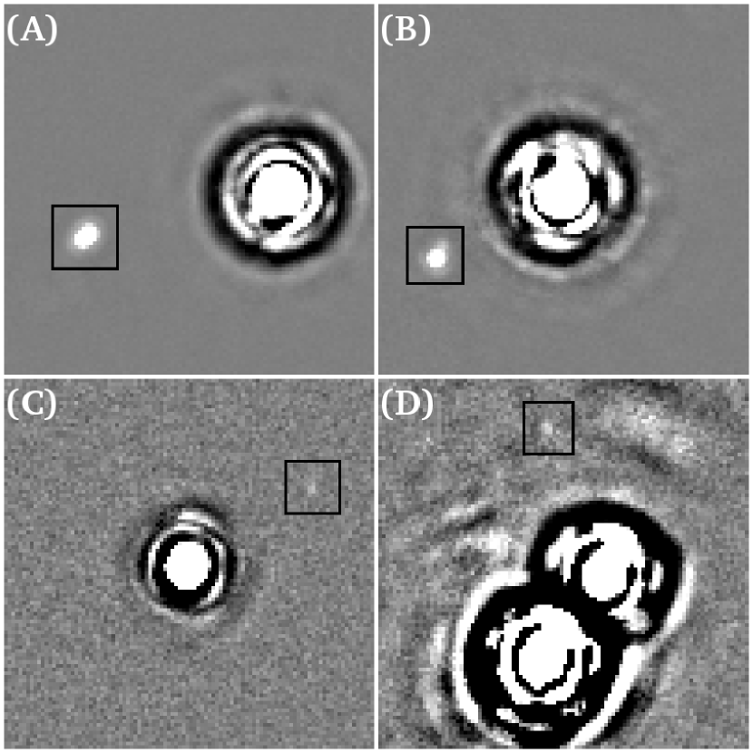
Figure 10: (A) $L^{\prime}$ image of GJ 564, showing the binary brown dwarf discovered by Potter et al. (2003). (B) $L^{\prime}$ image of GJ 3876, showing the low-mass stellar companion we discovered. (C) $L^{\prime}$ image of BD+60 1417, showing the faint background star we detected. (D) $L^{\prime}$ image of binary star GJ 684, showing the faint background star we detected. Each tile is 4.86 arcsec square; the bottom tiles are contrast stretched 10$\times$ more than the top ones to reveal the faint companions.

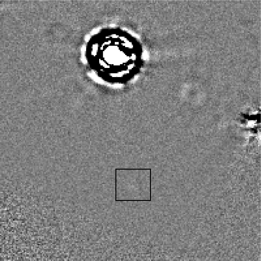
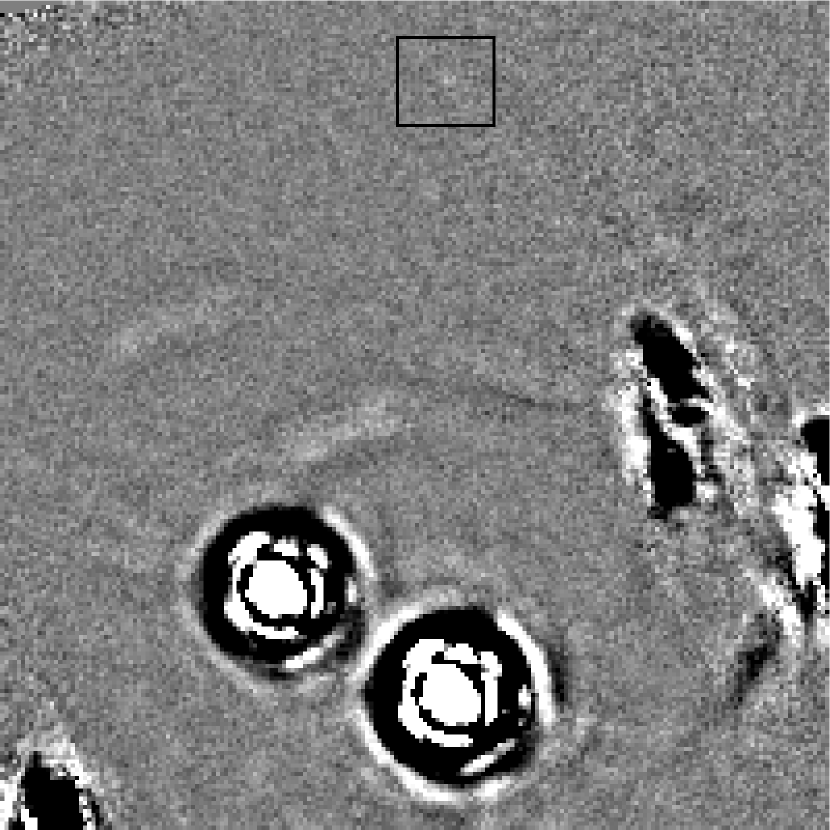
Figure 11: Left, $L^{\prime}$ image of GJ 354.1 A, showing the faint background star we detected. Right, $L^{\prime}$ image of binary star GJ 860, again showing a faint background star. Each image is 9.71 arcsec square, contrast stretched the same as the lower panels in Figure 10 to reveal the faint objects.

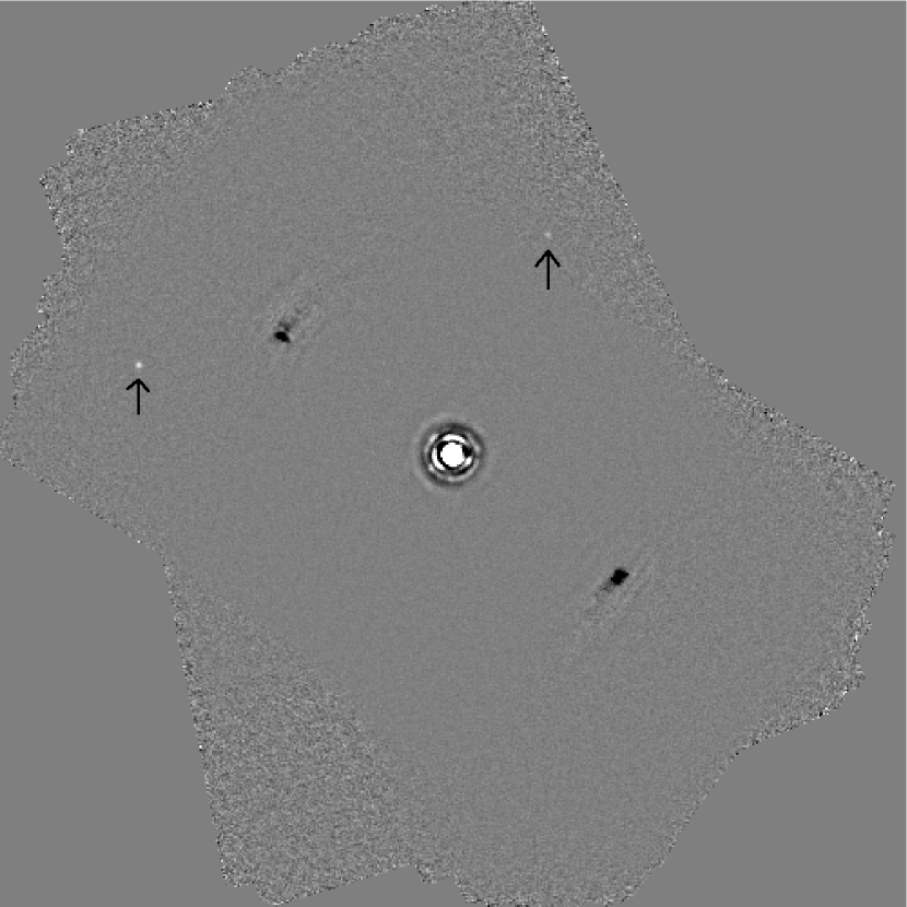
Figure 12: $L^{\prime}$ image of BD+20 1790, showing two faint background stars. Image is 24.29 arcsec square, contrast stretched 3$\times$ less than the images in Figure 11, to give a clear view of these somewhat brighter stars.

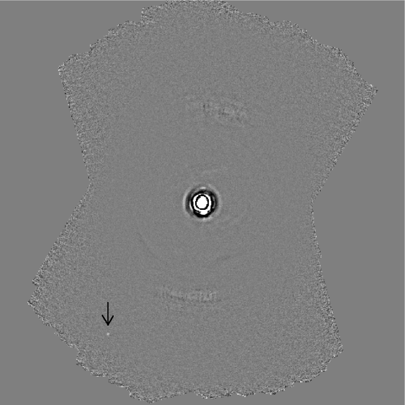
Figure 15: $L^{\prime}$ image of GJ 3860, showing a faint background star. Image is 24.29 arcsec square, contrast stretched the same as the previous figure.

5.2 The Low-Mass Star GJ 3876 B

The single discovery of our survey is the low-mass stellar companion of GJ 3876. We first detected it on $L^{\prime}$ images from April 13, 2006, and confirmed it as a common proper motion companion in $L^{\prime}$, $M$, and $K_{S}$ images taken on April 11, 2007. Table 11 gives our photometric and astrometric results, complete with what the object’s position should have been in April 2007 if it were a background star.

Table 11: Discovery Data for GJ 3876 B

Date	Sep	PA
(yyyy/mm/dd)	(arcsec)	(degrees)	$K_{S}$	$L^{\prime}$	$M$
2006/04/13	$1.8518\pm 0.0038$	$118.57\pm 0.19$	$\cdots$	$10.88\pm 0.06$	$\cdots$
2007/04/11	$1.8603\pm 0.0082$	$118.64\pm 0.24$	$11.51\pm 0.22$	$10.79\pm 0.08$	$10.91\pm 0.28$
Background	1.6487	113.73	$\cdots$	$\cdots$	$\cdots$

Note. — Astrometry and photometry of the single discovery of our survey, GJ 3876 B. The first two rows give actual measured values; the last gives the predicted position for 2007/04/11 if the object were a background star, based on the 2006/04/13 position and a proper motion measurement from Perryman et al. (1997). The background star hypothesis is rejected with great confidence.

GJ 3876 B is clearly a common proper motion companion. The distance to the primary star is about 43 pc, based on the parallax from Perryman et al. (1997). This translates to a projected separation of about 80 AU, which suggests an orbital period of around 700 yr for a one solar mass primary. The constant position angle over a year seems inconsistent with a face-on orbit at this period, while the formally insignificant increase in separation may hint at motion in a more inclined orbit – however, much more data is needed.

Again using the Perryman et al. (1997) distance, the $K_{S}$ absolute magnitude of GJ 3876 B is $8.33\pm 0.22$. Based on the models of Baraffe et al. (1998), this translates into a mass of about $0.15\pm 0.01$M_☉. This estimate could be further investigated using our $L^{\prime}$ and $M$ band magnitudes, but model magnitudes for low mass stars in these bands are not readily available in the literature, and integrating them from theoretical spectra is beyond the scope of this paper.

5.3 Astrometry of Known Bright Binaries

We calibrated the plate scale and orientation of the Clio camera using observations of known wide, very long-period binary stars. We had previously obtained precise astrometry of these stars in the optical using the University of Arizona’s 61 inch Kuiper telescope on Mt. Bigelow (Heinze et al. (2009); for more complete data see http://www.hopewriter.com/Astronomyfiles/AstrometryPoster.html).

When selecting our survey sample, we rejected some binary stars with orbital properties that seemed likely to destabilize any planets we could detect. After these rejections, twenty stars in known binary systems remained in our sample. Since our AO images allow very accurate astrometry, which might be useful for refining the orbital parameters of these nearby binaries, we present our measurements of them in Table 12.

Note that these binary stars change position relatively quickly, and should not be used for calibration except with a precise orbital solution. Those referred to in Heinze et al. (2009) and the associated website are better for calibration purposes, but some of them may still have moved significantly since our measurements.

The measurements in Table 12 are averages of astrometry based on individual frames. In many cases we had short, unsaturated images available in addition to our longer, saturated exposures for planet detection. This allowed us to compare the internal precision of both saturated and unsaturated images, and choose as our final astrometric result the average of whichever of the two image sets had the smaller internal scatter. As explained in Section 3.3, the agreement between saturated and unsaturated astrometry was generally excellent. Note that the Table 12 value for our $L^{\prime}$ observations of $\xi$ Boo is based on unsaturated images; this was the binary star with the largest (though still only 0.009 arcsec) saturated/unsaturated difference in the list given in Section 3.3. The uncertainties given in Table 12 combine both measurement scatter and calibration uncertainty. The latter is generally the larger term, due to the necessity of calibrating Clio using less precise astrometry from seeing-limited optical observations. The true internal scatter of carefully conducted astrometric observations using Clio and MMTAO is certainly several times smaller than the uncertainties quoted in the table. Despite the calibration uncertainties, however, clear orbital motion in the star GJ 702 is seen over an interval of only ten months. See Heinze et al. (2009) and the previously-cited website for an analysis of the challenges and potential of using AO astrometry for binary star orbital science.

Table 12: Astrometry of Binary Survey Targets

	Date Obs.
Star Name	(yyyy/mm/dd)	Sep.(arcsec)	PA(deg)
GJ 166 BC	2006/12/03	$8.781\pm 0.010$	153.72 $\pm$ 0.20
HD 77407 AB	2007/01/05	$1.698\pm 0.004$	356.37 $\pm$ 0.20
HD 96064 AB	2007/01/04	$11.628\pm 0.007$	221.61 $\pm$ 0.20
HD 96064 Bab	2007/01/04	$0.217\pm 0.010$	26.60 $\pm$ 4.30
GJ 505 AB	2006/06/12	$7.512\pm 0.006$	104.92 $\pm$ 0.20
$\xi$ Boo AB	2006/06/10	$6.345\pm 0.006$	312.15 $\pm$ 0.20
$\xi$ Boo AB ($M$)	2006/06/11	$6.327\pm 0.005$	312.14 $\pm$ 0.20
GJ 684 AB	2006/06/11	$1.344\pm 0.004$	323.84 $\pm$ 0.20
GJ 702 AB	2006/06/09	$5.160\pm 0.005$	135.79 $\pm$ 0.20
GJ 702 AB ($M$)	2007/04/11	$5.290\pm 0.004$	134.69 $\pm$ 0.20
GJ 860 AB	2006/06/12	$2.386\pm 0.004$	58.55 $\pm$ 0.20
GJ 896 AB	2006/07/13	$5.366\pm 0.006$	86.16 $\pm$ 0.20
HD 220140 AB	2006/12/03	$10.828\pm 0.007$	214.49 $\pm$ 0.20

Note. — The internal precision of Clio astrometry is considerably better than the uncertainties given here, especially for the position angles. Calibration uncertainty is important since we had to calibrate the detector from seeing-limited optical astrometry of wide binaries. Even so, GJ 702 shows clear orbital motion in the 10 months spanned by our two measurements.

6 Conclusion

We have surveyed unusually nearby, mature star systems for extrasolar planets in the $L^{\prime}$ and $M$ bands using the Clio camera with the MMT AO system. We have developed a sophisticated image processing pipeline for data from this camera, including some interesting innovations. We have carefully and rigorously analyzed our sensitivity. Accurately determining the sensitivity of AO planet-search images is a more complex task than, perhaps, has been widely appreciated. Our data support the conclusion of Marois et al. (2008) that $5\sigma$ limits can substantially overestimate the meaningful sensitivity of an image. Blind tests involving fake planets inserted in raw data are the best way to confirm the validity of any sensitivity estimator, and should be included in all future planet-search publications. By extensive use of such tests, we established a definitive significance vs. completeness relation for planets in our data. This relation is important for use in Monte Carlo simulations to constrain planet distributions.

We have discovered a physically orbiting $\sim 0.15$M_☉ binary companion at a projected separation of 80 AU from the star GJ 3876. We have detected twelve additional candidate faint companions, one of which is the binary brown dwarf companion of GJ 564 discovered prior to our observations by Potter et al. (2003). The remaining eleven are confirmed to be background stars. We note that shorter wavelength surveys, such as that of Lafrenière et al. (2007) in the $H$ band regime, have typically found a much larger number of background stars, necessitating extensive follow-up observations. A long wavelength survey such as ours can obtain good sensitivity to planets, with their very red IR colors, while remaining blind to all but the brightest stars. This reduces the amount of telescope time spent following up planet candidates that turn out to be background stars.

We did not detect any planets, but have set interesting limits on the masses of planets or other substellar objects that may exist in the star sytems we surveyed. In Heinze et al. (2010), we use extensive Monte Carlo simulations to show how our null result constrains the mass and semimajor axis distributions of extrasolar planets orbiting sun-like stars.

7 Acknowledgements

This research has made use of the SIMBAD online database, operated at CDS, Strasbourg, France, and the VizieR online database (see Ochsenbein et al (2000)).

We have also made extensive use of information and code from Press et al. (1992).

We have used digitized images from the Palomar Sky Survey (available from http://stdatu.stsci.edu/cgi-bin/dss_form), which were produced at the Space Telescope Science Institute under U.S. Government grant NAG W-2166. The images of these surveys are based on photographic data obtained using the Oschin Schmidt Telescope on Palomar Mountain and the UK Schmidt Telescope.

We thank the anonymous referee for helpful suggestions.

Facilities: MMT, SO:Kuiper

References

- Barrado y Navascués (1998) Barrado y Navascués, D. 1998, A&A, 339, 831
- Baraffe et al. (2003) Baraffe, I., Chabrier, G., Barman, T. S., Allard, F., & Hauschildt, P. H. 2003, A&A, 402, 701
- Baraffe et al. (1998) Baraffe, I., Chabrier, G., Allard, F., Hauschildt, P. H. 1998, A&A, 337, 403
- Biller et al. (2007) Biller, B. A., Close, L. M., Masciadri, E., Nielsen, E., Lenzen, R., Brandner, W., McCarthy, D., Hartung, M., Kellner, S., Mamajek, E., Henning, T., Miller, D., Kenworthy, M., & Kulesa, C. 2007, ApJS, 173, 143
- Bouchy et al. (2009) Bouchy, F., Mayor, M., Lovis, C., Udry, S., Benz, W., Bertaux, J.-L., Delfosse, X., Mordasini, C., Pepe, F., Queloz, D., & Segransan, D. 2009, A&A, 496, 527
- Bryden et al. (2006) Bryden, G., Beichman, C. A., Trilling, D. E., Rieke, G. H., Holmes, E. K., Lawler, S. M., Stapelfeldt, K. R., Werner, M. W., Gautier, T. N., Blaylock, M., Gordon, K. D., Stansberry, J. A., & Su, K. Y. L. 2006, ApJ, 636, 1098
- Burrows et al. (2003) Burrows, A., Sudarsky, D., & Lunine, J. I. 2003, ApJ, 596, 578
- Butler et al. (2006) Butler, R. P., Wright, J. T., Marcy, G. W., Fischer, D. A., Vogt, S. S., Tinney, C. G., Jones, H. R. A., Carter, B. D., Johnson, J. A., McCarthy, C., & Penny, A. J. 2006, ApJ, 646, 505.
- Chauvin et al. (2010) Chauvin, G., Lagrange, A.-M., Bonavita, M., Zuckerman, B., Dumas, C., Bessell, M.S., Beuzit, J.-L., Bonnefoy, M., Desidera, S., Farihi, J., Lowrance, P., Mouillet, D. & Song, I. 2010, A&A, 509, A52
- Cox (2000) Cox, A. N. 2000, Allen’s Astrophysical Quantities (Fourth Edition; New York, NY: Springer-Verlag New York, Inc.)
- Cumming et al. (2008) Cumming, A., Butler, R. P., Marcy, G. W., Vogt, S. S., Wright, J. T., & Fischer, D. A. 2008, PASP, 120, 531.
- Cutri et al. (2003) Cutri, R., Skrutskie, M., van Dyk, S., Beichman, C., Carpenter, J., Chester, T., Cambresy, L., Evans, T., Fowler, J., Gizis, J., Howard, E., Huchra, J., Jarett, T., Kopan, E., Kirkpatrick, J., Light, R., Marsh, K., McCallon, H., Schneider, S., Stiening, R., Sykes, M., Weinberg, M., Wheaton, W., Wheelock, S., & Zacarias, N. 2003, 2MASSS All Sky Catlog of point sources (The IRSA 2MASS All-Sky Point Source Catalog, NASA/IPAC Infrared Science Archive. http://irsa.ipac.caltech.edu/applications/Gator/)
- Favata et al. (1998) Favata, F., Micela, G., Sciortino, S., & D’Antona, F. 1998, A&A, 335, 218
- Fischer (1998) Fischer, D. 1998, PhD Thesis entitled Lithium Abundances in Field K Dwarfs, University of California Santa Cruz
- Fischer & Valenti (2005) Fischer, D. A. & Valenti, J. 2005, ApJ, 622, 1102
- Fitzgerald & Graham (2006) Fitzgerald, M. P., & Graham, J. R. 2006, ApJ, 637, 541
- Freed et al. (2004) Freed, M., Hinz, P., Meyer, M., Milton, N., & Lloyd-Hart, M. 2004, Proc. SPIE, 5492, 1561
- Gomes et al. (2005) Gomes, R., Levison, H., Tsiganis, K., & Morbidelli, A. 2005, Nature, 435, 466
- Heinze et al. (2008) Heinze, A. N., Hinz, P. M., Kenworthy, M., Miller, D., & Sivanandam, S. 2008, ApJ, 688, 583
- Heinze et al. (2009) Heinze, A. N., Hinz, P. M., Sivanandam, S. 2009, BAAS, 41, 300
- Heinze et al. (2010) Heinze, A. N., Hinz, P. M., Kenworthy, M., Meyer, M., Sivanandam, S., & Miller, D. 2010, ApJ, in press
- Hernandez et al. (2000) Hernandez, X., Valls-Gabaud, D., & Gilmore, G. 2000, MNRAS, 316, 605
- Hinz et al. (2006) Hinz, P., Heinze, A., Sivanandam, S., Miller, D., Kenworthy, M., Brusa, G., Freed, M., & Angel, J. 2006, ApJ, 653, 1486.
- Hünsch et al. (1998) Hünsch, M., Schmitt, J., Sterzik, M. & Voges, W. 1998, Astron. Astrophys. Suppl. Ser. 135, 319
- Juric & Tremaine (2008) Juric, M. & Tremaine, S. 2008, ApJ, 686, 603
- Kasper et al. (2007) Kasper, M., Apai, D. Janson, M. & Brandner, W. 2007, A&A, 472, 321
- Kenworthy et al. (2007) Kenworthy, M., Codona, J., Johanan, L., Hinz, P., Angel, J., Heinze, A., & Sivanandam, S. 2007, ApJ, 660, 762
- King et al. (2003) King, J., Villarreal, A., Soderblom, D., Gulliver, A., & Adelman, S. 2003, ApJ, 125,1980
- Lafrenière et al. (2007) Lafrenière, D., Doyon, R., Marois, C., Nadeau, D., Oppenheimer, B., Roche, P., Rigaut, F., Graham, J., Jayawardhana, R., Johnstone, D., Kalas, P., Macintosh, B., & Racine, R. 2007, ApJ, 670, 1367
- López-Santiago et al. (2006) López-Santiago, J., Montes, D., Crespo-Chacón, I., & Fernández-Figueroa, M. J. 2006, ApJ, 643, 1160
- Lowrance et al. (2005) Lowrance, P., Becklin, E., Schneider, G., Kirkpatrick, J., Weinberger, A., Zuckerman, B., Dumas, C., Beuzit, J., Plait, P., Malumuth, E., Heap, S., Terrile, R., & Hines, D. 2005, AJ, 130, 1845
- Mamajek et al. (2009) Mamajek, E., Soderblom, D., & Wyse, R. 2009, in The Ages of Stars, ed. E. E. Mamajek, D. R. Soderblom, & R. F. G. Wyse (Cambridge: Cambridge University Press)
- Marley et al. (2007) Marley, M. S., Fortney, J. J., Hubickyj, O., Bodenheimer, P., & Lissauer, J. J. 2007, ApJ, 655, 541
- Marois et al. (2006) Marois, C., Lafrenière, D., Doyon, R., Macintosh, B., & Nadeau, D. 2006, ApJ, 641, 556
- Marois et al. (2008) Marois, C., Lafrenière, D., Macintosh, B., & Doyon, R. 2008, ApJ, 673, 647
- Masciadri et al. (2005) Masciadri, E.; Mundt, R.; Henning, Th.; Alvarez, C.; & Barrado y Navascués, D 2005, ApJ, 625, 1004
- Montes et al. (2001) Montes, D., López-Santiago, J., Fernaández-Figueroa, M., & Gálvez, M. 2001, A&A, 379, 976
- Ochsenbein et al (2000) Ochsenbein, F., Bauer, P. & Marcout, J. 2000, ApJS, 143, 23O
- Potter et al. (2003) Potter, D., Cushing, M., & Neuhauser, R. 2003, in The Future of Cool-Star Astrophysics: 12th Cambridge Workshop on Cool Stars, Stellar Systems, and the Sun, ed. A. Brown, G.M. Harper, and T.R. Ayres, (University of Colorado), p 689-693
- Perryman et al. (1997) Perryman, M., Lindegren, L., Kovalevsky, J., Hog, E., Bastian, U., Bernacca, P., Creze, M., Donati, F., Grenon, M., Grewing, M., Van Leeuwen, F., Van Der Marel, H., Mignard, F., Murray, C., Le Poole, R., Schrijver, H., Turon, C., Arenou, F., Froeschle, M., & Peterson, C. 1997, A&A, 323, L49
- Press et al. (1992) Press, W. H., Teukolsky, S.A., Vetterling, W. T., & Flannery, B. P. 1992, Numerical Recipes in C (Second Edition; New York, NY: Cambridge University Press)
- Sivanandam et al. (2006) Sivanandam, S., Hinz, P., Heinze, A., & Freed, M. 2006, Proc. SPIE, 6269, 27
- Soummer et al. (2007) Soummer, R., Ferrari, A., Claude, A., & Jolissaint, L. 2007, ApJ, 669,642
- Wichmann et al. (2003) Wichmann, R., Schmitt, J., & Hubrig, S. 2003, A&A, 399, 983
- Wichmann & Schmitt (2003) Wichmann, R. & Schmitt, J. 2003, MNRAS, 342, 1021
- Zuckerman et al. (2001) Zuckerman, B., Song, I., Bessell, M., & Webb, R. 2001, ApJ, 562, L87