Probing decoherence through Fano resonances

Abstract

We investigate the effect of decoherence on Fano resonances in wave transmission through resonant scattering structures. We show that the Fano asymmetry parameter $q$ follows, as a function of the strength of decoherence, trajectories in the complex plane that reveal detailed information on the underlying decoherence process. Dissipation and unitary dephasing give rise to manifestly different trajectories. Our predictions are successfully tested against microwave experiments using metal cavities with different absorption coefficients and against previously published data on transport through quantum dots. These results open up new possibilities for studying the effect of decoherence in a wide array of physical systems where Fano resonances are present.

One of the central issues of current research in quantum mechanics is decoherence Zurek (2006), i.e., the loss of coherence induced in a system by the interaction with its environment. Studying the ubiquituous effects of decoherence is not only of fundamental interest for the understanding of the quantum–to–classical crossover, but is the key to the realization of operating quantum information devices which rely on long coherence times Bouwmeester et al. (2000); birdreview . To this end, decohering processes need to be controlled and suppressed. In practice, however, enumeration and identification of sources of decoherence is already a challenging task on its own (see, e.g., Simmonds et al. (2004); gurvitz ). This is, in part, due to the fact that different decoherence channels are difficult to distinguish from one another since their influence on the observables of interest is often very similar.

Decoherence in quantum systems is, typically, described within the framework of an open quantum system approach by a quantum master equation of, e.g., the Lindblad form lindblad . In this framework the reduced density operator, $\rho$, of the open system with Hamiltonian $H_{S}$ interacting with the environment through Lindblad operators $L_{j}$ evolves as,

$$i\dot{\rho}=\left[H_{S},\rho\right]+i\left[\sum_{j}L^{\phantom{\dagger}}_{j}\rho L^{\dagger}_{j}-\frac{1}{2}\left(L^{\dagger}_{j}L^{\phantom{\dagger}}_{j}\rho+\rho L^{\dagger}_{j}L^{\phantom{\dagger}}_{j}\right)\right]\,.$$ (1)

The system-environment interactions allow for a decohering, yet unitary evolution of the system within the Markov approximation. In the special case that only the last term of the coupling in Eq. (1) $(\sim L^{\dagger}_{j}L^{\phantom{\dagger}}_{j}\rho+\rho L^{\dagger}_{j}L^{\phantom{\dagger}}_{j})$ is present, interaction with the environment is purely dissipative. The counter-term $(\sim L^{\phantom{\dagger}}_{j}\rho L^{\dagger}_{j})$ acts as source and preserves the unitarity of the evolution. Characterizing the system-environment interaction for a given physical realization is one of the major challenges of decoherence theory. In this letter we show that Fano resonances, specifically the asymmetry parameter $q$, allow to disentangle different decoherence mechanisms present in resonant scattering devices such as quantum dots gurvitz ; goeres2000 ; Kobayashi et al. (2003); Johnson et al. (2004); gong (for a review see fanoreview ). The $q$ parameter follows, as a function of the decoherence strength, trajectories in the complex plane that are specific to the underlying environmental coupling. In particular, dissipation and decoherent dephasing can be distinguished from each other.

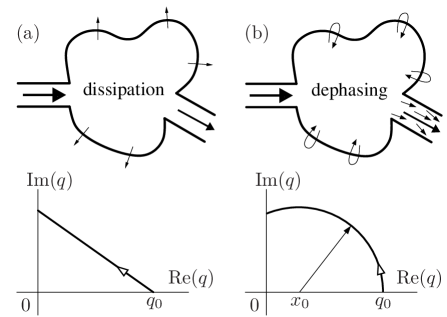
Figure 1: Dependence of the complex Fano asymmetry parameter $q$ on the decoherence strength $\chi$. In the case of a uniformly dissipative system (a) an increase of $\chi$ shifts $q(\chi)$ in the complex plane along a straight line away from a real value $q_{0}$ while for a uniformly dephasing system (b) the trajectory $q(\chi)$ forms a circular arc. This arc is centered at $x_{0}$ on the real axis thus featuring a vertical tangent at $q_{0}$.

Fano line shapes in transport result from the interference between different channels in the transmission amplitude Fano (1961),

$$t(k)=z_{r}\,\frac{\Gamma/2}{k-k_{\rm res}+i\Gamma/2}+t_{d}\,,$$ (2)

with $t_{d}$ the amplitude of a (smoothly varying) direct (or background) channel and $z_{r}$ the strength, $k_{\rm res}$ the position, and $\Gamma$ the width of the resonant channel. The transmission probability in the vicinity of the resonance, $|t(k)|^{2}$ takes on the form of a Fano profile,

$$|t(k)|^{2}=|t_{d}|^{2}\frac{|\,\varepsilon+q\,|^{2}}{1+\varepsilon^{2}},$$ (3)

in terms of the reduced wavenumber (or energy) $\varepsilon=(k-k_{\rm res})/(\Gamma/2)$. The asymmetry parameter $q$ determines the shape of the Fano resonance. In the limit $q\!\to\!\pm\infty$, the symmetric Breit-Wigner shape is recovered while for $q\!\to\!0$ window (or “anti”) resonances appear. For single-channel scattering through systems with time-reversal symmetry (TRS) $q$ is strictly real footnote ; lewenkopf . When TRS is broken, Eq. (3) still holds, but $q$ may take on complex values Clerk et al. (2001). The generalization of the Fano $q$ parameter is therefore ideally suited as a sensitive probe of TRS-breaking processes. An Aharonov-Bohm ring exposed to a TRS-breaking magnetic field was recently shown to exhibit $q$ parameters performing periodic oscillations in the complex plane Kobayashi et al. (2003). Decoherence, being a prime example for breaking TRS, should leave distinct signatures in the behavior of $q$ as well Kobayashi et al. (2003); Johnson et al. (2004); Clerk et al. (2001); Rotter et al. (2005); Zhang and Chandrasekhar (2006); gong . In the present letter we provide experimental and theoretical evidence that the complex $q$-trajectory reveals details on the underlying decoherence process that are characteristically different for dissipation and irreversible dephasing.

We first consider ballistic transport through a scattering cavity in the presence of uniform dissipation, the strength of which is independent of the wavelength or position inside the cavity [Fig. 1(a)]. For the corresponding open quantum system this corresponds to the reduction of the coupling to the environment [Eq. (1)] to sink terms $(\sim L^{\dagger}_{j}L^{\phantom{\dagger}}_{j}\rho+\rho L^{\dagger}_{j}L^{\phantom{\dagger}}_{j})$ only. Physical realizations of pure dissipation in quantum dots include electron-hole recombination and currents leaking into the substrate. For classical wave scattering Jackson (1998) the presence of dissipation in a resonant device shifts the resonance positions $k_{\rm res}\rightarrow\overline{k}_{\rm res}=$ $k_{\rm res}-\Delta k-i\kappa$. Since, in relative terms, the broadening of the resonance width $\kappa$ usually dominantes over $\Delta k$, Eq. (2) is modified as follows,

$$t(k)\approx z_{r}\,\frac{\Gamma/2}{k-k_{\rm res}+i\Gamma/2+i\kappa}+t_{d}\,,$$ (4)

with a broadened resonance width ($\Gamma+2\kappa$).

As convenient measure for the strength of decoherence we use the ratio $\chi=2\kappa/(\Gamma+2\kappa)$, with the limiting cases $\chi=0$ in the absence of decoherence and $\chi=1$ for dissipation-dominated broadening. With Eq. (4) the generalized $q$ parameter in Eq. (3) now becomes,

$$q(\chi)=q_{0}+\chi(i-q_{0})\,,$$ (5)

where $q_{0}$ is the real $q$ parameter in the absence of dissipation. For increasing dissipation strength the complex Fano $q$ parameter follows a straight line trajectory in the complex plane [see Fig. 1(a)] which, for large dissipation strength ($\chi\rightarrow 1$), approaches the limit $q=i$. The linear form of $q(\chi)$ follows from the assumption entering Eq. (4) that only the resonant but not the direct amplitude ($t_{d}$) is affected by decoherence—an assumption which generally holds well for resonant scattering devices (including microwave cavities).

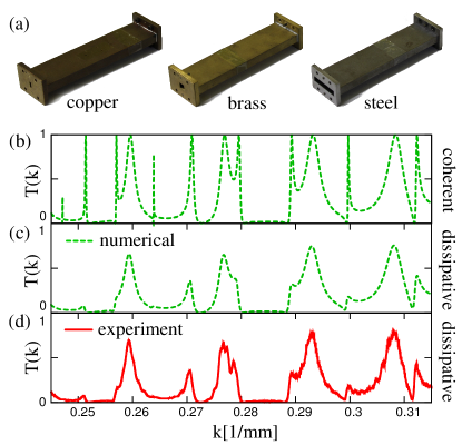
Figure 2: (Color online) (a) Rectangular microwave cavities of identical dimensions but out of different materials. The left two cavities are shown with a shutter at the opening as used for tuning the Fano parameter. (b)-(d) Wavenumber dependence of transmission $T(k)$ through a cavity. In (b) the fully coherent limit is shown. (c) and (d) display the transmission with the dissipative decoherence as present in the steel cavity at room temperature. Theoretical MRGM (c) and experimental data (d) show excellent agreement on an absolute scale.

The analytical dependence of $q$ on the decoherence strength has previously been studied in the case of dephasing [Fig. 1(b)] as the main source of decoherence Clerk et al. (2001). Here, in contrast to the dissipative case, the flux in the system is conserved even at finite coherence lengths. A simple realization of flux-conserving decoherent dephasing for ballistic transport is given by the Büttiker dephasing probe Büttiker (1986): By attaching a fictitious voltage probe, the coherent scattering paths from source to drain are accompanied by incoherent paths via the voltage probe which randomize the phase information. To convert the dissipative voltage probe into a flux-conserving dephasing probe, the potential of the probe is chosen such that the flux leaving through the probe is incoherently injected back into the cavity. This corresponds to the presence of both sink and source terms in the Liouvillian operator [Eq. (1)] with an infinite number ($j=1,\ldots,\infty$) of coupling terms with random phases. Such an incoherent reinjection of flux is fully accounted for by an additional Breit-Wigner shaped term in the Fano profile,

$$|t(k)|^{2}=|t_{d}|^{2}\left[\frac{\left\{\,\varepsilon^{\prime}+{\rm Re}[q(\chi)]\,\right\}^{2}}{1+\varepsilon^{\prime 2}}+\frac{{\rm Im}[q(\chi)]^{2}}{1+\varepsilon^{\prime 2}}\right]\,,$$ (6)

with the reduced wavenumber now rescaled to the increased resonance width $\varepsilon^{\prime}=(k-k_{\rm res})/(\Gamma/2+\kappa)$ as well as ${\rm Re}[q(\chi)]=q_{0}(1-\chi)$ and ${\rm Im}[q(\chi)]^{2}=\chi\left[1+q_{0}^{2}(1-\right.$ $\left.\chi)\right]$. By eliminating $\chi$ from these expressions, one finds

$$\left\{{\rm Re}[q(\chi)]-x_{0}\right\}^{2}+{\rm Im}[q(\chi)]^{2}=r^{2}_{0}\,,$$ (7)

where $x_{0}=[q_{0}-1/q_{0}]/2$ and $r^{2}_{0}=1+x_{0}^{2}$ are independent of $\chi$. Thus $q(\chi)$ describes a circle in the complex plane centered at $(x_{0},0)$ on the real axis and converging to $q(\chi\!\to\!1)=i$ [see Fig. 1(b)]. We find circular trajectories in the complex $q$-plane also for a different (more general) scenario of dephasing modeled by gradually suppressing the interference term between the direct and the resonant transmission in Eq. (2) as $\chi\!\to\!1$ (for details see appendix). Also here the circle is centered on the real axis, but imaginary values for $q(\chi\!\to\!1)$ may differ from $i$.

We conclude that for the same Fano resonance as determined by the $q(\chi\!\to\!0)=q_{0}$ limit, the complex generalization of $q$ evolves along different trajectories for finite $\chi$ for purely dissipative (on a straight line) and dephasing (on a circular arc) decoherence. Even for small $\chi$ where $q$ is close to the real axis characteristic differences appear: the dephasing trajectory has a tangent parallel to the imaginary axis while the dissipative trajectory takes off at an angle $\arctan(1/q_{0})$ relative to the $x$-axis. This finding suggests that by following the $q(\chi)$ trajectory for a given Fano resonance, the underlying decoherence process can be unambiguously identified.

An ideal system for the controlled experimental verification of the above theoretical results are microwave cavities which have been successfully employed in the past as analog simulators of a wide variety of quantum transport phenomena stoeckmannbook . As was shown recently, well-separated Fano resonances can be measured with high accuracy in such systems Rotter et al. (2005). The transport of microwaves into and out of the cavity can be controlled via shutters at both ends, which in turn determine the $q_{0}$ values of resonances. Due to the finite conductivity of the cavity and the resulting dissipation of flux in the cavity walls, decoherence is naturally present. Furthermore, we can control the degree of dissipation by cooling the cavities to lower temperatures or by fabricating cavities with identical geometry out of different materials. To a good degree of approximation, the power loss can be assumed to be uniform and mode-independent [as in Eq. (4)].

For the experiment we used rectangular microwave cavities (length $L=176\,$mm, width $D=39\,$mm) [see Fig. 2(a)] made out of copper, brass and steel with different conductivities $\sigma$ [at room temperature: $\sigma=54.22\,\mathrm{m}/(\Omega\,\mathrm{mm}^{2})$ for copper, $\sigma=12.20\,\mathrm{m}/(\Omega\,\mathrm{mm}^{2})$ for brass, and $\sigma=1.37\,\mathrm{m}/(\Omega\,\mathrm{mm}^{2})$ for steel]. The cavities were terminated by two metallic shutters each with opening width $s=8.8\,$mm and a thickness of $1\,$mm. Two aluminum leads with length $l=200\,$mm and width $d=15.8\,$mm were attached to the openings. The measurements were carried out using a microwave vector analyzer connected via coaxial cables and adapters at the end of each lead. We note that the measuring device is thus “part of the semi-infinite lead” and not an additional measurement channel gurvitz . Measurements were performed in the frequency range with exactly one transverse mode in each lead thus coupling to the first and third transverse modes of the cavity (see Ref. Rotter et al. (2005) for details).

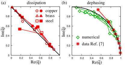
Figure 3: (Color online) (a) Complex Fano $q$ parameter extracted from microwave experiments on copper, brass and steel cavities. For each material, measurements were performed at room temperature (filled symbols) and liquid nitrogen temperature (open symbols). (b) Fano parameter corresponding to the theoretical MRGM data for a dephasing cavity (diamond symbols) and the experimental data from Ref. goeres2000 (asterisk symbols). Data points for the same resonance at different decoherence strengths are connected by colored lines and rescaled, $q\!\to\!\tilde{q}$, to reach $\tilde{q}=1$ $(\tilde{q}=i)$ in the fully coherent (incoherent) limit. The straight [circular] black curve in (a) [(b)] displays the theoretical prediction following Eq. (5) [Eq. (7)] for the case of uniform dissipation [dephasing].

The experimental transmission data $T(k)=|t(k)|^{2}$ recorded for the steel cavity display well-separated Fano resonances [see Fig. 2(d)]. For comparison we also show the corresponding numerical results including dissipation [see Fig. 2(c)] and without dissipation [see Fig. 2(b)]. The numerical data was obtained with the modular recursive Green’s function method (MRGM) Rotter et al. (2000), where uniform microwave attenuation by dissipation following Jackson (1998) was taken into account. Even though the effect of dissipation is quite sizeable, we find excellent agreement between theory and experiment [see Figs. 2(c),(d)]. The small oscillations in the experimental data not reproduced by the numerical calculations can be attributed to standing waves induced by the minimal reflection from the adapters (less than 1%). The influence on the Fano resonances is, however, negligible as compared to the dominant decoherence process, i.e., the ohmic losses in the cavity walls. Accordingly, Eq. (5) predicts the $q$ parameters of Fano resonances to display linear decoherence trajectories in the complex plane. To verify this prediction, we now extract the complex Fano $q$ parameter from resonances at different decoherence strengths as determined by the different cavity materials and their temperature dependence (on each cavity one measurement was performed at ambient temperature and at liquid nitrogen cooling). Since the Fano resonance formulas Eqs. (2),(3) are strictly only valid for a direct amplitude $t_{d}$ which is $k$-independent, we exclude resonances from our analysis for which this requirement is not satisfied. For resonances satisfying this requirement we extract the $q$ parameters by selecting the minimum, maximum and one intermediate value as fitting points in the experimental transmission probabilities [as, e.g., in Fig. 2(d)]. Following each resonance for different degrees of dissipation thus allows us to obtain the desired decoherence trajectories in the complex $q$ plane. To facilitate the comparison of the behavior of different members of the ensemble of resonances we rescale all data [$q\!\to\!\tilde{q}={\rm Re}(q)\,q^{-1}_{0}+i\,{\rm Im}(q)$] onto a single “universal” trajectory which connects the points $\tilde{q}=1$ and $\tilde{q}=i$. The data shown in Fig. 3(a) demonstrates that the expected linear behavior is, indeed, observed.

Such a linear trajectory due to pure dissipation can now be contrasted with the circular trajectory for flux-conserving dephasing. For open quantum systems this corresponds to the presence of an infinite number of source $(\sim L^{\phantom{\dagger}}_{j}\rho L^{\dagger}_{j})$ and sink terms $(\sim L^{\dagger}_{j}L^{\phantom{\dagger}}_{j}\rho+\rho L^{\dagger}_{j}L^{\phantom{\dagger}}_{j})$ in Eq. (1) as induced, e.g., by wave number independent electron-phonon coupling. In the classical electromagnetic cavity such a flux-restoring incoherent source is difficult to realize. However, in our simulation we can numerically reinject the dissipated power into the rectangular cavity, leaving the scattering system otherwise unchanged. The dissipated flux to be symmetrically reinjected is determined as the difference between transmission plus reflection and the unitary limit, $1-|t(k)|^{2}-|r(k)|^{2}$. The $q$ values extracted from the numerically determined Fano profiles are also mapped onto a “universal” circular arc with radius 1 centered at $x_{0}=0$. The data obtained for several Fano resonances closely follow the circular trajectory [Fig. 3(b)] confirming the dependence of the $q(\chi)$ trajectory on the underlying decoherence mechanism.

To test our predictions also for a true quantum scattering system, we reanalyzed published experimental data on Fano resonances in transport through resonant quantum dots goeres2000 . For these conductance measurements in the temperature range 100mK $\leq T\leq$ 800mK, we find the evolution of $q(T)$ in the complex plane to be very well described by a circular arc (see Fig. 3b)—as predicted for flux-preserving dephasing. Details of this analysis as well as a comparison between the experimental and the theoretical Fano resonance curves are provided in the appendix.

In conclusion, we have demonstrated that Fano resonances may serve as sensitive probes of decoherence in wave transport. We find that for increasing dephasing or dissipation strength the Fano asymmetry parameter $q$ evolves on circular arcs or on straight lines in the complex plane. As confirmed by measurements on microwave cavities and on quantum dots, these characteristic signatures provide a means to determine not only the degree but also the specific type of decoherence present in the experiment. It is hoped that the present findings will stimulate future experimental investigations of the influence of decoherence on the Fano $q$-parameter in resonant quantum transport.

Appendix with supplementary material

Appendix A Complex $q$-trajectories: the case of dephasing

Following previous analysis Clerk et al. (2001) based on the Büttiker dephasing probe model, we show in the main text of our article that for this specific model the Fano $q$-parameter follows a circular trajectory in the complex plane. It is now instructive to inquire whether this result can also be found for a more general scenario of dephasing. One such generic approach is the ensemble average over a random phase $\phi$ between the resonant ($\propto z_{r}$) and the background amplitude $t_{d}$,

$$t=t_{d}+\frac{z_{r}}{i+\varepsilon}\,e^{i\phi}\,,$$

where the reduced wavenumber $\varepsilon=(k-k_{\rm res})/(\Gamma/2)$, see Eq. (3). With the random phase $\phi$ featuring a zero mean and a standard deviation $\sigma$ the interference term in the ensemble average of the total transmission $\langle|t|^{2}\rangle_{\phi}$ will be gradually suppressed for increasing $\sigma$. This behavior can be conveniently described by a prefactor $(1-\chi)\in[0,1]$, containing the dephasing strength $\chi(\sigma)$,

$$\begin{split}\langle|t|^{2}\rangle_{\phi}&=|t_{d}|^{2}+\frac{|z_{r}|^{2}}{1+\varepsilon^{2}}+(1-\chi)\,2\mathrm{Re}\left(t_{d}^{*}\,\frac{z_{r}}{i+\varepsilon}\right)\\ &=|t_{d}|^{2}\,\frac{|z_{r}/t_{d}|^{2}+(1-\chi)\,2\mathrm{Re}\left[\frac{z_{r}}{t_{d}}(-i+\varepsilon)\right]+(1+\varepsilon^{2})}{1+\varepsilon^{2}}\,.\end{split}$$

The limit of complete dephasing ($\chi\rightarrow 1$) corresponds to the incoherent addition of resonant and background contribution. With the real value of the Fano parameter $q_{0}$ in the absence of decoherence given as $q_{0}=i+z_{r}/t_{d}$ Clerk et al. (2001), we further obtain,

$$\begin{split}\langle|t|^{2}\rangle_{\phi}=|t_{d}|^{2}\,\frac{\left[\varepsilon+(1-\chi)q_{0}\right]^{2}-(1-\chi)^{2}q_{0}^{2}+q_{0}^{2}+2\chi}{1+\varepsilon^{2}}\,.\end{split}$$

Comparing this expression with the general form of a Fano resonance as in Eq. (6) reveals the evolution of the complex Fano parameter $q(\chi)$ as a function of the decoherence strength $\chi$,

$$\mathrm{Re}[q(\chi)] =(1-\chi)\,q_{0}\,,$$

$$\mathrm{Im}[q(\chi)]^{2} =2\chi+q_{0}^{2}\,(2\chi-\chi^{2})\,.$$

Eliminating $\chi$ from the above two equations finally yields,

$$\mathrm{Im}[q(\chi)]^{2}+\{\mathrm{Re}[q(\chi)]+1/q_{0}\}^{2}=2+\frac{1}{q_{0}^{2}}+q_{0}^{2}\,,$$

which describes a circle in the complex plane with radius $r_{0}=\sqrt{2+1/q_{0}^{2}+q_{0}^{2}}$, centered at $x_{0}=-1/q_{0}$ on the real axis. Note that in the limit of complete dephasing ($\chi\to 1$) the above trajectory $q(\chi)$ converges to a value on the imaginary axis which, in contrast to the result obtained with the Büttiker dephasing probe model Clerk et al. (2001), is not necessarily given by $q=i$.

We thus arrive at the interesting conclusion that different models of dephasing may yield a similar circular behavior of $q(\chi)$ where, however, the radius of the circular arc and its corresponding end point depend on the specific dephasing scenario.

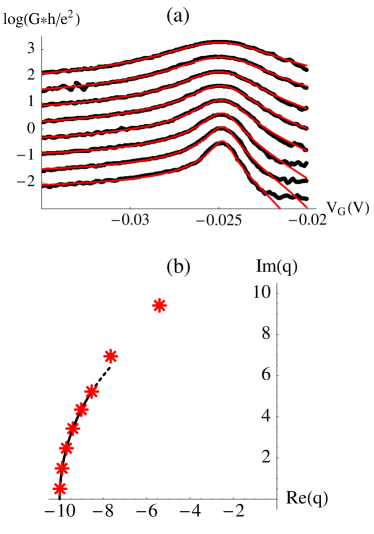
Figure 4: (a) Voltage dependence of the conductance through a resonant quantum dot as measured in the experiment by Zacharia et al. goeres2000 . The black dots show the values extracted from goeres2000 in steps of 100 mK between 100mK (lowest curve) and 800mK (highest curve). For better visibility the data sets with $T>$ 100 mK are each multiplied by a factor of $\sqrt{10}$ from one temperature value to the next. The red curves show the analytical curves resulting from restricted parameter fits (see text) with the corresponding complex $q$-values being displayed in (b) by the red asterisk symbols. The black curve in (b) shows a circular arc as prescribed for the dephasing model of decoherence.

Appendix B Details on the employed fitting procedures

When extracting the complex value of $q$ from a resonance profile, the imaginary part of $q$ is highly sensitive to the minimum value of the profile. General automated fitting routines, however, do typically not account for this specific dependence appropriately. To overcome this difficulty we used the minimum, maximum, and an intermediate point of the resonance as interpolation points in our procedure. Furthermore, we took advantage of the knowledge that the minimum and maximum points are extreme values of the Fano resonance, resulting in altogether five equations. Their solution yields the resonance amplitude, the resonance position $k_{\rm res}$, the resonance width $\Gamma$ and the real and imaginary part of $q$. All the $q$-values in Fig. 3 corresponding to the microwave experiment and to the numerical dephasing data were extracted in this way. Resonances with a non-uniform background were excluded from our analysis.

As outlined in the main text, we also tested our predictions against experimental data previously published in goeres2000 . In that publication the resonant conductance through a quantum dot was studied as a function of temperature $T$ (100mK $\leq T\leq$ 800mK). The corresponding experimental data extracted directly from goeres2000 are shown in Fig. 4(a) (black dots), right above. Unfortunately, for all the resonance curves provided in goeres2000 the background transmission is very small, such that the corresponding Fano resonance lineshapes in the conductance are very near the symmetric Breit-Wigner limit (with $|q|\gg 1$). In this limit we find rigorous multi-parameter fits with a complex-valued $q$-parameter as performed on the more asymmetric Fano resonances (with $|q|\lesssim 1$ as in the microwave data) to be unfeasible. This is because for $|q|\gg 1$ the symmetry-restoring effect of decoherence is hard to quantify. To test if the quantum dot data can be described by our theoretical predictions, we instead performed a consistency check whether a trajectory $q(\chi)$ can be found that features good agreement with both the experimental data and a circular form of $q(\chi)$. For this purpose we carried out restricted parameter fits which, in line with goeres2000 , were performed on a logarithmic conductance scale with thermal broadening being included separately and the data for the fit being restricted to the range where the conductance is at least twice as large as the measured conductance minimum (to reduce the influence of neighboring peaks). The best curves which we found in this way are shown in Fig. 4(a) (red lines) with the corresponding $q$-values shown in Fig. 4(b) (red symbols) and in Fig. 3(b) (after rescaling to the unit circle). The overall very good agreement demonstrates that the arc-like behavior of $q(\chi)$ can very well describe the experimental data. To cross-check this result we also mapped the measurement data on a linear $q(\chi)$-trajectory (not shown) as prescribed by the dissipation-dominated decoherence in Eq. (5) and found much larger discrepancies. We hope future quantum transport experiments will make more asymmetric Fano resonances (with $|q|\lesssim 1$) available for rigorous analysis.

References

- Zurek (2006) W. H. Zurek, Rev. Mod. Phys. 75, 715 (2003).
- Bouwmeester et al. (2000) D. Bouwmeester, A. Ekert, and A. Zeilinger, The physics of quantum information (Springer, 2000).
- (3) J. J. Lin and J. P. Bird, J. Phys.: Condens. Matter 14, R501 (2002).
- Simmonds et al. (2004) R. Simmonds et al., Phys. Rev. Lett. 93, 077003 (2004).
- (5) B. Elattari and S. A. Gurvitz, Phys. Rev. Lett. 84, 2047 (2000); J. Z. Bernád, A. Bodor, T. Geszti, and L. Diósi, Phys. Rev. B 77, 073311 (2008).
- (6) G. Lindblad, Commun. Math. Phys. 48 119 (1976).
- (7) I. G. Zacharia et al., Phys. Rev. B 64, 155311 (2001).
- Kobayashi et al. (2003) K. Kobayashi, H. Aikawa, S. Katsumoto, and Y. Iye, Phys. Rev. Lett. 88, 256806 (2002); Phys. Rev. B 68, 235304 (2003).
- Johnson et al. (2004) A. C. Johnson, C. M. Marcus, M. P. Hanson, and A. C. Gossard, Phys. Rev. Lett. 93, 106803 (2004).
- (10) W. Gong and Y. Zheng and J. Wang and T. Lü, Phys. Status Solidi B 245, 1175 (2008).
- (11) A. E. Miroshnichenko, S. Flach, and Y. S. Kivshar, arXiv:0902.3014.
- Fano (1961) U. Fano, Phys. Rev. 124, 1866 (1961).
- (13) Note that the -parameter is complex for multi-channel scattering with TRS lewenkopf (a case not considered here).
- (14) M. Mendoza et al., Phys. Rev. B 77, 155307 (2008).
- Clerk et al. (2001) A. A. Clerk, X. Waintal, and P. W. Brouwer, Phys. Rev. Lett. 86, 4636 (2001).
- Zhang and Chandrasekhar (2006) Z. Zhang and V. Chandrasekhar, Phys. Rev. B 73, 075421 (2006).
- Rotter et al. (2005) S. Rotter et al., Phys. Rev. E 69, 046208 (2004); Physica E 29, 325 (2005).
- Jackson (1998) J. D. Jackson, Classical Electrodynamics (Wiley, 1998).
- Büttiker (1986) M. Büttiker, Phys. Rev. B 33, 3020 (1986); IBM J. Res. Dev. 32, 63 (1988).
- (20) H. J. Stöckmann Quantum Chaos: An Introduction (Cambridge University Press, Cambridge, 1999).
- Rotter et al. (2000) S. Rotter et al., Phys. Rev. B 62, 1950 (2000); ibid. 68, 165302 (2003).