Automatic analysis of distance bounding protocols

Abstract

Distance bounding protocols are used by nodes in wireless networks for the crucial purpose of estimating their distances to other nodes. This typically involves sending a request by one node to another node, receiving a response, and then calculating an upper bound on the distance by multiplying the round-trip time with the velocity of the signal. However, dishonest nodes in the network can turn the calculations both illegitimate and inaccurate when they participate in protocol executions. Therefore, it is important to analyze protocols for the possibility of such violations. Past efforts to analyze distance bounding protocols have only been manual. However, automated approaches are important since they are quite likely to find flaws that manual approaches cannot, as witnessed many times in the literature of key establishment protocols.

In this paper, we use the constraint solver tool to automatically analyze distance bounding protocols: We first formulate a new trace property called   Secure Distance Bounding (SDB)   that protocol executions must satisfy. We then classify the scenarios in which these protocols can operate considering the (dis)honesty of nodes and location of the attacker in the network. Finally, we extend the constraint solver tool so that it can be used to test protocols for violations of SDB in those scenarios and illustrate our technique on several examples that include new attacks on published protocols. We also hosted an on-line demo for the reader to check out our implementation.

Sreekanth Malladi, Bezawada Bruhadeshwar^†, Kishore Kothapalli

1 Introduction

A   distance bounding (DB) protocol   is used by a   “verifier”   node in wireless networks to calculate an upper bound on the distance to a   “prover”   node in the network. Distance bounding helps in crucial applications such as localization, location discovery and time synchronization. Hence, the security of DB protocols is an important and critical problem.

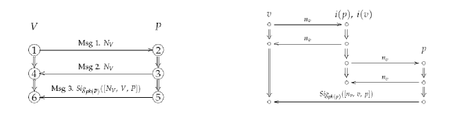
Figure 1:   (a)   Extended Echo protocol P1        (b)   Man-in-the-Middle Attack on P1

As an example of a DB protocol, consider a simple extension of the Echo protocol (Fig. 1.a) presented in [11]. In the figure,   ${\mathit{{\mathbf{missing}}}}{V}$   is the verifier,   ${P}$   is the prover;   $N_{V}$   is a nonce;   ${\mathit{Sig}}_{{\mathit{pk}}(P)}([N_{V},~{}V,~{}P])$   is the signature of   $P$   to be verified with it’s public-key, denoted   ${\mathit{pk}}(P)$. Let   $t_{i}$   be the time on the clock when event   $i$   occurs. Then,   $V$   can calculate the bound   ‘$d$’   on the distance to   $P$   as:   $d=\frac{(t_{4}-t_{1})~{}-~{}(t_{3}-t_{2})}{2}~{}~{}\times~{}~{}s$,   where   ‘$s$’   is the speed of the signal.

In the presence of attackers, DB protocols can fail to achieve their main goal of establishing a valid distance bound. For instance, the above protocol has a possible attack wherein an attacker   ${i}$   plays Man-In-The-Middle and succeeds in showing   ${p}$   as being closer to   ${v}$   than it really is (Fig. 1.b).

Analysis of DB protocols involves examining whether it is possible to make a party appear closer than it really is, to an honest verifier. The problem is different and difficult compared to standard Dolev-Yao analysis of protocols that only consider whether an attacker can generate messages required to violate some security property. Here, we need to factor in the time required for message generation as well, which can vary based on the input size and cryptographic parameters. Automated analysis is much desired, given the problems and distrust in manual analysis of protocols that have been reported in literature [5]. There have been numerous instances when automated techniques found attacks on protocols that manual, hand-based techniques could not (e.g. [6, 7, 9]).

Past work.

The few published efforts to analyze DB protocols have been largely incomplete: The classical work of Brands and Chaum [2] is mostly informal and specific to the protocols introduced in that paper. Sastry et al. [11] show that in their “Echo” protocol, the prover cannot respond before receiving the verifier’s nonce but the protocol is used only for “in-range” verification and also too simple without any authentication. Meadows et al. [8] give a method to analyze both distance bounding and authentication aspects, but the method like the previous two, is manual, not automated.

Our contribution.

To address these concerns, we will show a method to automatically analyze DB protocols using the constraint solving technique of Millen-Shmatikov. Our method is based on formal modeling of timed protocols and distance bounding properties. Further, it is fully automated with minor changes to the existing constraint solver. Some highlights of our contribution are:

1. Like many past strand space extensions, our formal modeling and framework give a simple, clean and useful geometric flavor to the study of DB protocols that could be used or extended to many other studies such as localization algorithms;

2. Some properties we prove about DB protocols allow the use of conventional Dolev-Yao style analysis, completely eliminating the need to consider the more complicated timing aspects. This is useful when it is difficult to extend existing methods for conventional key establishment protocols to analyze or verify DB protocols (e.g. ProVerif [1]).

Organization.

We will first develop a timed protocol model extending strand spaces in Section 2. We will then explain how constraint solving can be used to generate timed protocol executions in Section 3. We will formalize secure distance bounding and explain our technique to detect violations for it in Section 4. We will identify the scenarios under which DB protocols need to be analyzed in Section 5. We will illustrate our analysis approach on some examples in Section 6, and conclude with a discussion of future and related works.

2 Protocol model - Timed strand spaces

Our protocol model is based on the strand space model of [14] extended with the introduction of a new field,   “time”   for labels on nodes. This field is used to represent the current time on the clock at the node for an agent.

Definition 2.1.

[Node]   A   node   is a 3-tuple with fields   time,   sign,   and   term.   Time is the current time on the clock, sign can be   $+$   or   $-$   denoting   “send”   and   “receive”   respectively and term to be defined next.

We will describe how to populate the times on nodes partly in this section and partly in the next section. We consider protocols in which messages are constructed using a free term algebra:

Definition 2.2.

[Term]   A   term   is one of the following:   Variable   (can be of types   ${\mathit{Agent}}$,   ${\mathit{Nonce}}$   etc.);   Constant   (numbers   1, 2, $\ldots$; name of the attacker   $\epsilon$   etc.);   Atom;   Pair   denoted   $[t_{1},~{}t_{2}]$   if   $t_{1}$   and   $t_{2}$   are terms;   Public-Key   denoted   ${\mathit{pk}}(A)$   with   $A$   of type   ${\mathit{Agent}}$;   Shared-Key   denoted   ${\mathit{sh}}(A,B)$   with   $A$   and   $B$   of type   ${\mathit{Agent}}$;   Asymmetric encryption   denoted   $[t]^{\to}_{k}$   where   $t$   and   $k$   are terms;   Symmetric encryption   denoted   $[t]^{\leftrightarrow}_{k}$   where   $t$   and   $k$   are terms;   Hash   denoted   $h(t)$   where   $t$   is a term;   Signature   of a term   $t$   denoted   ${\mathit{Sig}}_{{\mathit{pk}}(A)}(t)$   to be validated using   ${\mathit{pk}}(A)$.

A   “ground”   term is any term with no variables in it. We will drop the superscript   $\to$   or   $\leftrightarrow$   if the mode of encryption is contextually either obvious or irrelevant.

Definition 2.3.

[Subterm]   Term   $t$   is a   subterm   of   $t^{\prime}$   (i.e.   $t\sqsubset t^{\prime})$   if   $t=t^{\prime}$,   or   if $t^{\prime}=[t_{1},t_{2}]$   with   $t\sqsubset t_{1}\vee t\sqsubset t_{2}$,   or   if $t^{\prime}=[t^{{}^{\prime\prime}}]_{k^{\prime}}$   with   $t\sqsubset t^{{}^{\prime\prime}}$,   or if   $t^{\prime}=h(t^{{}^{\prime\prime}})$   with   $t\sqsubset t^{{}^{\prime\prime}}$,   or if   $t^{\prime}={\mathit{Sig}}_{{\mathit{pk(A)}}}(t^{{}^{\prime\prime}})$   with   $t\sqsubset t^{{}^{\prime\prime}}$.   Term   $t$   is a   proper subterm   of   $t^{\prime}$   if   $(t\sqsubset t^{\prime})\wedge(t\neq t^{\prime})$.

Strands capture roles of a protocol.

Definition 2.4.

[Strand]   A   strand   is a sequence of nodes. For instance   $s=\langle n_{1},\ldots,n_{m}\rangle$   is a strand with $m$ nodes. Nodes in a strand are related by the edge   $\Rightarrow$   defined such that if   $n_{i}$   and   $n_{i+1}$   belong to the same strand, then   $n_{i}\Rightarrow n_{i+1}$.   A   parametric strand   is a strand with no atoms in the terms on its nodes.

Protocol roles are modeled as partially instantiated parametric strands that we name   semi-strands   where messages contain variables and atoms depending on the knowledge of agents concerning message subparts. For instance, the verifier strand of the protocol presented in the Introduction is represented as

$$\langle~{}~{}+[0,~{}n_{v}],~{}~{}-[T_{4},~{}n_{v}],~{}~{}-[T_{6},~{}{\mathit{Sig}}_{{\mathit{pk}}(P)}([n_{v},~{}v,~{}P])]~{}~{}\rangle$$

Notice that the first node starts at time   ‘0’   which is not a universal   ‘0’   but a local start time for the agent who dons this strand. Also notice that the times on the other two nodes   $T_{4}$   and   $T_{6}$   are not fixed. The rationale for this is to be explained shortly.

A set of semi-strands is called a   semi-bundle.   We will say that term $t$ belongs to a semi-bundle   $S$   (i.e.   $t\in S$)   if   $(t=\mathrm{term}(n))$   for some   $(n\in s)$   and   $(s\in S)$.

A   bundle   is a possible protocol execution obtained by consistently instantiating all the variables in the semi-bundle and using   $\to$   edges between nodes on different strands.

Definition 2.5.

[Bundle]   A   bundle   is a collection of strands and an acyclic digraph defined on a mapping of nodes to edges   $\to$   and   $\Rightarrow$   such that if node   $n_{i}$   sends a message that   $n_{j}$   receives, then   $n_{i},~{}~{}n_{j}$   are related by the edge   $\to$   (denoted   $n_{i}\to n_{j}$).   Further, if there is a node   $n$   in the bundle that receives a term   $t$,   then there is another node   $m$   in the bundle, that sends   $t$   such that   $m\to n$.

Note that this bundle is a 3-dimensional graph with strands located vertically anywhere in the cube. Nodes in a bundle are also related by precedence relation denoted   $\preceq$   which is a partial order:

Definition 2.6.

[Precedes]   The relation   $\preceq$   is defined such that if nodes   $n_{i},~{}~{}n_{j}$   exist in a bundle   $\mathcal{C}$,   then   $n_{i}\preceq n_{j}$   if they are on the same strand with   $i\leq j$;   further,   $n_{i}\prec n_{j}$   if   $n_{i}\to n_{j}$.

We will use   $\preceq$   on stand-alone strands in semi-bundles as well: Let   $s$   be a strand in a semi-bundle   $S$.   Then,   $(\forall n_{i},n_{j}\in s)(s\in S)(i\leq j\Rightarrow n_{i}\preceq n_{j})$.

We do not include the notion of penetrator strands as in the classical strand spaces formalism of [14]. Rather, we consider a single penetrator also modeled as a single strand that captures all the   “penetrator actions”   in the bundle defined as below:

Definition 2.7.

[Penetrator action]   A   penetrator action   is a sequence of edges   $t_{1}\to t_{2}\Rightarrow t_{3}\to t_{4}$   where   $t_{2}\Rightarrow t_{3}$   is an edge on the penetrator strand.

The idea is that the single   $\Rightarrow$   edge in a penetrator action represents all the penetrator strands in the classical model of [14] to generate the term to be sent. Multiple penetrators could be added in the 3-dimensional cube if desired, although we only consider a single “Machiavellian” attacker with full control of the network in the spirit of [13].

Next we define the   “elapsed time”   between any two nodes   $n_{i},~{}~{}n_{j}$   in a bundle   $C$   with   $n_{i}\preceq n_{j}$   using the notion of   weights   and   paths:

Definition 2.8.

[Weight or Elapsed time]   The   weight   of an edge is the (absolute) difference in times between the nodes that are connected by the edge. A   path   is a sequence of nodes such that every node in the sequence is related to the subsequent node by a   $\to$   or a   $\Rightarrow$.   The weight of a path is the sum of the weights of all the edges in the path.

We will denote the path between   $n_{i}$   and   $n_{j}$   as   $(n_{i},~{}n_{j})$   when there is only one route between   $n_{i}$,   and   $n_{j}$.

The weight of a   $\pm t\Rightarrow+t^{\prime}$   edge should be preset and constant for each semi-strand. In the case of penetrator strand, those weights should be calculated using penetrator actions required to generate the   $+$   node. On the other hand, the weight of a   $\pm t\Rightarrow-t^{\prime}$   edge cannot be fixed since an agent can only know the length of time after which it sends a message, but cannot always predict when it might receive a message from another agent, accurately.

Weights of   $\to$   edges indicate the time of traversal for messages which depends on the message length, distance and the velocity of the signal. We assume that there is an appropriate formula for an environment to calculate the weight of these edges, using those parameters.

Definition 2.9.

[Relay,   Simple relay]   A   relay   is a penetrator action   $+t\to-t\Rightarrow+t\to-t$.   A   simple relay   is a relay with the weight of the   $\Rightarrow$   edge being zero.

We develop the notion of   “ideal”   and   “real”   bundles to distinguish protocol executions where the penetrator plays a passive role of merely observing message exchanges between agents with those where she plays an active role of faking and changing messages.

Definition 2.10.

[Ideal and Real bundles]   An   ideal bundle   $B$   for a protocol   $P$   is a bundle formed from a semi-bundle   $S$   with exactly one semi-strand per parametric strand of   $P$   where every penetrator action is a simple relay   $+\sigma t\to-\sigma t\Rightarrow+\sigma t\to-\sigma t$   for some substitution   $\sigma$   such that   $(\forall s\in S)((\exists s^{\prime}\in B)(s^{\prime}=\sigma s))$.   A   real bundle   is any bundle from any other semi-bundle from   $P$.

3 Extending constraint solving to find elapsed time

We will now extend the constraint solving technique of [9] to give a “recipe” to produce the timed bundles defined in Section 2 including honest strands and the single penetrator strand with all the penetrator actions.

The previous section only noted that weights of   $\pm\Rightarrow+$   edges should be preset; this section will complete labeling of nodes since weights on   $\pm\Rightarrow-$   edges are calculated dynamically setting the times on   ‘$-$’   nodes during protocol executions. The elapsed time between any two nodes in such bundles can then be calculated by summing up the weights on all the edges in the path between the nodes.

Constraint solving is a procedure to determine if a semi-bundle is completable to a bundle using a substitution to variables. A constraint sequence is first drawn from node interleavings of the semi-bundle indicating that   ‘$-$’   nodes should be derivable by the attacker with his actions and terms on all prior   ‘$+$’   nodes.

Definition 3.1.

[Constraint sequence]   A   constraint sequence   $C=\langle~{}\mathrm{term}(n_{1})~{}:~{}T_{1},~{}\ldots,$ $~{}\mathrm{term}(n_{k})~{}:~{}T_{k}~{}\rangle$   is from a semi-bundle   $S$   with   $k$   ‘$-$’   nodes if   $(\forall~{}n,~{}n^{\prime})(~{}((\mathrm{term}(n^{\prime})~{}:~{}T\in C)$ $\wedge(\mathrm{term}(n)\in T))\Rightarrow(n\preceq n^{\prime})~{})$.   Further, if   $i<j$   and   $n_{i}$,   $n_{j}$   belong to the same strand, then   $n_{i}\preceq n_{j}$   and   $(\forall i)(T_{i}\subseteq T_{i+1})$.

We consider a set of attacker operators   $\Phi$   and an infinite set of terms that can built using   $\Phi$   on a finite set of terms   $T$,   denoted   $\mathcal{F}(T)$.   Although our techniques in this paper are largely independent of the kind of operators in   $\Phi$,   we will consider that they represent the standard Dolev-Yao attacker as defined in [9].

The possibility of forming bundles from a given semi-bundle can be determined by testing if constraint sequences from it are satisfiable:

Definition 3.2.

[Satisfiability,   Realizability]   A constraint is   $m:T$   is   satisfiable   under a substitution   $\sigma$   if   $\sigma m\in\mathcal{F}(T)$.   A constraint sequence is   satisfiable   with   $\sigma$,   denoted   $\sigma\vdash C$   if   $(\forall m:T\in C)(\sigma m\in\mathcal{F}(\sigma T))$.   A   ‘$-$’   node is   realizable   if the corresponding constraint is satisfiable.   A semi-bundle is   completable   to a bundle if a constraint sequence from it is satisfiable.

Millen-Shmatikov have shown a constraint satisfaction procedure, denoted   P   that is terminating, sound and complete wrt   $\Phi$   and   $\mathcal{F}$.   P   applies a set of symbolic reduction rules   $R$   to each constraint, in order to reduce it them to   “simple constraints”   (with only a variable each on the left side). We provide both   P   and   $R$   in Appendix A.

We will consider that each reduction rule in   $R$   corresponds to an attacker action and we will calculate the weights of   $\Rightarrow$   edges of a bundle to be the sum of the times taken by each rule.

In Appendix A we also give an algorithm denoted   PB   that produces timed bundles as defined in Section 2, using   P   to calculate the weights of   $\Rightarrow$   edges. An example bundle generated for the Lowe’s attack on the NSPK protocol [5] is also given in Appendix A.4. Further, we show in Appendix B, Theorem B.1 that   PB   terminates and is sound and complete.

4 Analyzing DB protocols

We will now formalize secure distance bounding using the concept of ideal and real bundles defined in Section 2.

4.1 Formalizing Secure Distance Bounding

A DB protocol is used by a verifier   $v$   to establish an upper bound on the distance to a prover   $p$.   Ideally, if the following assumptions hold:     (a)   The positions of   $v$   and   $p$   are fixed,   (b)   The intervals between creating and sending messages are fixed,   (c)   $v$,   $p$   are honest and   (d)   There is no attacker;    then there indeed exists an upper bound on the distance that can be calculated by calculating the elapsed time between two nodes   ${\mathit{Request}}$   and   ${\mathit{Response}}$   on   $v$   with   ${\mathit{Request}}$   a send node,   ${\mathit{Response}}$   a receive node and   ${\mathit{Request}}\prec{\mathit{Response}}$   as explained in Section 2.

We will call the nodes between   ${\mathit{Request}}$   and   ${\mathit{Response}}$   in the verifier strand of a DB protocol as the   “DB part”   and the other nodes as the   “authentication part”.   Further, we will use the term   “Time of Flight”   or its abbreviation as   ToF   to refer to the elapsed time between   ${\mathit{Request}}$   and   ${\mathit{Response}}$.

Now the upper bound that is calculated by   $v$   can be lowered compared to the one obtained under ideal conditions, if    (a)   the ToF between its   ${\mathit{Request}}$   and   ${\mathit{Response}}$   is lowered   and    (b)   if $v$ is sent all the messages in the protocol that it expects to receive from   $p$.

This is the main insight in defining secure distance bounding as a trace property: We first calculate the   ToF   under ideal conditions and check whether a   “real”   execution of the protocol in the presence of the penetrator can result in a calculation of ToF that is lower than the ideal value. Note that we assume weights of   $\pm m\Rightarrow+m^{\prime}$   edges are set for strands in semi-bundles, by following the same measures to calculate time taken for message construction outlined in Section 3.

Definition 4.1.

[Secure Distance Bounding (SDB)]   Let   $t$   and   $t^{\prime}$   be the elapsed times in the verifier strand of an ideal and real bundle   ($B$   and   $B^{\prime}$)   respectively from a semi-bundle   $S$,   between the   ${\mathit{Request}}$   and   ${\mathit{Response}}$   nodes. Then   Secure Distance Bounding (SDB)   is satisfied in   $B^{\prime}$,   whenever   $t<t^{\prime}$.   Conversely,   SDB   is violated in   $B^{\prime}$   if   $t>t^{\prime}$.

This definition is dependent on what we consider an ideal bundle to be. In Section 2, we defined it to be one with no penetrator actions, but when the penetrator is further from   $v$ than $p$ is, we would need to make the bundle between the penetrator and $v$ as the ideal. More on this is explained in Section 5.2.

5 Protocol execution scenarios

Before explaining our technique to test protocols for violations of SDB, we will consider the scenarios under which a DB protocol can operate.

5.1 Scenarios based on honesty of the prover

We first consider scenarios in which the prover is honest or dishonest.

Scenario A (honest prover).

With the verifier, honest prover and an attacker, this scenario captures MITM/Mafia attacks [3]. The attack described in the Introduction is one such attack.

Scenario B (dishonest, colluding prover).

With the verifier, dishonest prover and attacker, this scenario captures terrorist/collusion attacks [3]. Here, the prover colludes with an attacker who is presumably closer to the verifier, by passing some or all of its information including secret keys and messages (partial or full collusion). The protocol in Section  1 is vulnerable to such an attack (Fig. 2.a).

Figure 2: (a) Scenario B — colluding attacker      (b) Scenario 2 — further attacker

5.2 Scenarios based on location of attacker

Independent of the honesty of agents, we should also categorize protocol execution scenarios based on the location of the attacker in the network with respect to the verifier and the prover.

Scenario 1 (closer attacker).

Attacker   $i$   physically closer to the verifier   $v$   than the prover   $p$   is. The first attack on   P1   described previously is an example for this scenario.

In this situation, we can show that     (a)    if an attacker can generate all the messages expected by the verifier from the   ${\mathit{Request}}$ to the   ${\mathit{Response}}$   without those messages being sent by the prover   and     (b)    if all other messages expected by the verifier can also be generated by the attacker (with or without those messages emanating from the prover),    then SDB is violated:

Theorem 5.1.

Suppose   $t_{0},~{}t_{1},~{}\ldots,~{}t_{m}$   are terms on   $m$   nodes on the verifier strand   $v$   with time of flight measured in between   $t_{0}$   and   $t_{m}$.   Then, there exists a bundle with a violation of SDB if

• the constraints   $\langle~{}t_{1}~{}:~{}T_{0},~{}\ldots~{},~{}t_{m}:T_{m}~{}\rangle$ are satisfiable where for   $i=0$ to $m$,   every   $t\in T_{i}$   either belongs to   $T_{0}$   or a   $+$   node on   $v$   and every   $t_{i}$   is a term on a   $-$   node on   $v$;

• all other   $-$   nodes in   $v$   are realizable.

Proof 5.2.

Please see Appendix B, Theorem B.3.

Scenario 2 (farther attacker).

Attacker   $i$   is physically farther from   $v$   than   $p$.   Here,   $i$   tries to show itself closer to   $v$   by using the responses from   $p$   to   $v$   in the DB part, and then inserts its own messages for the authentication part.   P1   is vulnerable in this scenario as well (Fig. 2.b).

This scenario is exactly opposite of Scenario 1: we just have to assume that the ideal bundle now is in between   $v$   and   $i$   instead of   $v$   and   $p$.   We should then analyze protocols for potential executions with   $p$   sending all the messages in the DB part and attacker sending the remaining messages. We prove this below:

Theorem 5.3.

Consider   $v,~{}p_{1},~{}p_{2}$   where   $d(v,p_{1})<d(v,p_{2})$.   Let   $\langle~{}t_{0},~{}\ldots,~{}t_{m}~{}\rangle$   be nodes on   $v$   between which time of flight is measured. Then, there is a violation of SDB if

• the constraints   $\langle~{}t_{1}~{}:~{}T_{1},~{}\ldots,~{}t_{m}~{}:~{}T_{m}~{}\rangle$   are satisfiable where for all   $i=1$ to $m$,   every   $t_{i}$   is unified with some   $t^{\prime}_{1}\in T_{i}$   where   $t^{\prime}_{i}$   is a term on   $p_{1}$.

• All other   ‘$-$’   nodes of   $v$   are realizable without unifying with any subterms of   $p_{1}$.

Proof 5.4.

Please see Appendix B, Theorem B.5.

6 Implementation and Examples

We now present some example protocols and their analyses using our technique. We tested all the protocols in the Constraint Solver tool with the scenarios and results in Section 5. We hosted all the protocols and scenarios in our on-line demo which can be tested with the click of a button. Here, we will present only the most interesting attacks and at least one per type of scenario.

It is worth mentioning that we made a simple change to the solver: we restricted it to consider only those node interleavings wherein the   ${\mathit{Request}}$   and   ${\mathit{Response}}$   nodes in the verifier strand immediately follow each other. We show in Appendix C that this is required to ensure soundness and that it preserves completeness wrt Def 4.1.

In all the protocols below, distance bound,   $d=\frac{\delta_{1}~{}-~{}\delta_{2}}{2}\times s$   verifier fixes   $\delta_{2}$   as a constant for a given protocol. Further to save space, we simplified some bundles by removing simple and insignificant relays.

6.1 P2 - Brands and Chaum [2]

The original Brands-Chaum protocol is a bit tricky with commit, rapid bit-level exchange and authentication/sign phases, and XOR operator that is not modeled by the solver. Hence, we analyzed an approximate version (Fig. 3.a).

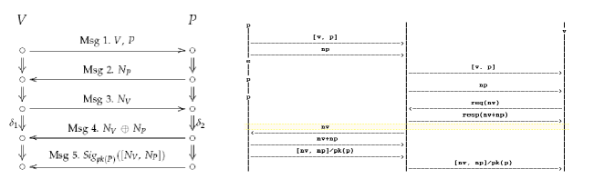
Figure 3: (a) Brands-Chaum protocol P2     (b) Actual solver trace of the MITM Attack on P2 (NOTE:   nv+np = $[n_{v}]^{\leftrightarrow}_{n_{p}}$, [nv,np]/pk(p) = ${\mathit{Sig}}_{{\mathit{pk}}(p)}[n_{v},~{}n_{p}]$;   ${\mathit{Request}}$   and   ${\mathit{Response}}$   nodes were coded as   req(nv)   and   resp(nv+np) )

Notice that there is a pre-commitment of nonce   $N_{P}$   by   $P$.   Brands and Chaum specify that messages 3 and 4 should be bit-by-bit exchanges with the round-trip time calculated as the average of all the bit exchanges. Since the exchange is rapid and no other messages can interfere during the exchange, we felt it safe to model the protocol with just one of those message exchanges. Also,   $N_{V}\oplus N_{P}$   was modeled as   $[N_{V}]^{\leftrightarrow}_{N_{P}}$.

Honest prover, Closer attacker.

Following our results in Section 5, we removed the nodes in the DB part in the prover strand and found an MITM attack on   P2   which was similar to the MITM attack on   P1   shown in the Introduction: Attacker simply sends all the messages except the signature to the verifier and later sends all of them to the prover. Finally, she relays the signature from the prover to the verifier. The solver found three different attack traces with three different node interleavings all essentially the same attack (Fig. 3.b).

The original Brands-Chaum protocol actually requires that the commitment   $N_{P}$   be secretly exchanged between   $V$   and   $P$.   With this requirement, the protocol forms a nice counter-example to Theorem 5.1: not all constraints corresponding to messages between Request (Msg 2) and Response (Msg 4) are satisfiable. When we made this change in the solver, it did not report an attack.

Dishonest prover, closer attacker.

Obviously, revealing the nonce   $N_{P}$   (the commitment) to the attacker before hand allowed the attack (partial collusion) and of course, full collusion worked too. In any case, Brands-Chaum seems stronger against collusion than   P1   since it requires sharing of   $N_{P}$   for the attack to succeed.

Farther attacker.

This protocol also forms a nice example to test under Scenario 2. Assuming that the attacker is further away from the verifier, we followed our guidelines in Section 5 and removed the nodes in the DB part in one strand, while removing the signature (Msg 5) in another strand. The solver then output an attack where the agent whose DB part was removed looks closer than it is to the verifier (see Appendix D).

6.2 P3 - Meadows et al. [8]

P3 below was recently proposed in [8] (Fig. 4.a).

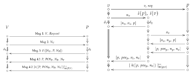
Figure 4:     (a)   Meadows et al. protocol P3                   (b)   MITM Attack

Honest prover, closer attacker.

P3   is actually quite similar to   P2   and Brands-Chaum but with some crucial changes. Even without any commitment step, it was not vulnerable to the MITM attack that we presented in Section 6.1 even though the nonce   $N_{P}$   is sent in plain in Msg 3 unlike Brands-Chaum that does not disclose it. This shows that sending   $N_{P}$   before   the   ${\mathit{Response}}$ (Msg 3)   was the fatal mistake in   P2.

In any case, thus we believe that   P3   is stronger than   P2   and also the Brands-Chaum protocol since it does not require a previous set up to enable secure commit.

Dishonest prover, closer attacker.

P3   is vulnerable with partial collusion when   $i$   responds with Msg 2 and forwards   $n_{v}$,   and   $n_{i}$   to   $p$   later so that it can send the signature in Msg 5 to   $v$   with   $n_{v}$,   $n_{i}$,   and other elements. However,   $p$   does not share any secrets with   $i$   to enable this attack. Hence, this protocol seems weaker than Brands-Chaum in this aspect.

Farther attacker.

P3   is also vulnerable to the   “nearest-neighbor”   attack that   P2   was, if we assume verifier does not know who it is talking to before receiving the signature in the final message. However, it would be unreasonable to make this assumption since the prover identity is explicitly included in the prior messages. Hence, we instantiated the prover variable   $P$   to a ground atomic value in the verifier strand when we tested this protocol, whence we could not reproduce the “nearest-neighbor” attack.

Tweaking P3.

Since the protocol was resistant to all other scenarios except collusion, we tweaked with the protocol to appreciate the significance of individual elements and their placement in messages. We could not find the use or purpose of the field ${\mathit{POS_{P}}}$ described anywhere in [8] but removing it did not reveal any new attack. It is interesting to ask if the nonce   $N_{P}$   inside Msg 4.2 is necessary. Removing it revealed an attack (Fig. 4.b).

6.3 P4 - Guttman et al. [4]

P4 differs from all others in having more than one encrypted message in the authentication part, seemingly extending the NSPK/NSL protocols (Fig. 5.a).

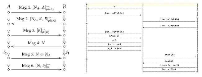
Figure 5:   (a)  Guttman et al. protocol P4         (b)   Screen-shot of attack trace from the solver on the new Guttman et al.’s protocol. Note:   v_1,   v_2 are variables;   [t]*k   =   $[t]^{\to}_{k}$,                 [t]+k   =   $[t]^{\leftrightarrow}_{k}$.

We analyzed this protocol with one strand per role in Scenarios A and 1; i.e. we considered an honest verifier   $B$   and an honest prover   $A$   with a MITM attacker who is physically in between them. Further, as usual, we tied the   ${\mathit{Request}}$ (Msg 4)   and   ${\mathit{Response}}$ (Msg 5)   together in the node interleaving. Without   ‘$B$’   in Msg 2, the solver reported the trace with a MITM attack termed “Lowe style” attack in [4] (Fig. 5.b).

In the trace, the attacker plays MITM between   $a$   and   $b$   and learns   $k$.   Then, the   ${\mathit{Response}}$   $[n,~{}n_{a}]$   is sent from the attacker’s location, which is physically closer to the verifier   $b$,   violating SDB and also follows it up with an authentication of the challenge   $n$   in the last message   ($[n,~{}\delta_{2}]^{\leftrightarrow}_{k}$).

The crux of this attack is the attacker’s ability to satisfy both the conditions in Theorem 5.1. Satisfying the DB Part is trivial, but satisfying the authentication part is possible only by breaking the secrecy of   $k$   since it is required to construct the last message,   $[n,~{}\delta_{2}]^{\leftrightarrow}_{k}$.

With larger semi-bundles/runs, more attacks could be possible by failing authentication even after the inclusion of   ‘$B$’   in Msg 2; E.g., see attacks on NSL given in [9].

7 Conclusion

In this paper, we described a method to automatically analyze distance bounding protocols. We formalized the main property of secure distance bounding and explained how violations of it can be tested using the constraint solver. We also illustrated our technique by presenting analyses of some published protocols.

A natural extension to our work is to extend it to unbounded analysis since the constraint solver only considers bounded number of protocol processes. Unbounded verification tools such as   ProVerif   could be extended by tying the Request and Rapid Response together in the node interleavings as explained in Section 6, to produce attacks or to prove the absence of. In the case of   ProVerif,   this is as simple as adding four events in the protocol, two each for the verifier and prover in the protocol, corresponding to sending and receiving the Request and Rapid Response respectively. No other change in the tool is required.

Other areas for future work include extending our framework with multiple penetrators in the 3D space, analyzing other properties in this model such as denial of service, obtaining decidability results for distance bounding, and testing protocols with a more powerful solver that considers message operators with algebraic properties such as Exclusive-OR.

Recent related work.

While the work in this paper was in progress, a related approach to verifying DB protocols using Isabelle/HOL was also in progress and is about to appear in [12]. Being a verification effort, that approach differs from ours in the classical way that model checkers differ from theorem provers: the former tests for attacks while the latter proves the absence of. However, our approach can also be extended easily to unbounded verification with   ProVerif,   as explained above.   ProVerif   usually verifies protocols in a fraction of a second, faster than most theorem provers. But to be fair to the authors of [12], they consider other protocols used in wireless networks, not merely distance bounding as we did. In that sense, their work can be considered more elaborate than ours.

Appendix A Constraint solving [9]

A.1 Reduction Procedure P

$C:=$ initial constraint sequence
$\sigma:=0$
repeat
let $c^{*}=m:T$ be	the constraint in $C$
	s.t. $m$ is not a variable
if $c^{*}$	not found
	output Satisfiable!
apply rule (elim) to $c^{*}$ until no longer applicable
$\forall r\in R$
if $r$	is applicable to $C$
	$\langle C^{\prime};\sigma^{\prime}\rangle:=r(C;\sigma)$
	create node with $C^{\prime}$; add $C\to C^{\prime}$ edge
	push $\langle C^{\prime};\sigma^{\prime}\rangle$
$\langle C;\sigma\rangle:=$ pop
until emptystack

Reduction Procedure P [9]

A.2 Set of reduction rules, $R$

$$\frac{C_{<},~{}m:T,~{}C_{>};~{}\sigma}{\tau C_{<},~{}\tau C_{>};~{}\tau~{}\cup~{}\sigma}~{}~{}\mathrm{where}~{}\tau=\mathrm{mgu}(m,t)\wedge t\in T~{}~{}~{}({\mathit{un}})$$

$$\frac{C_{<},~{}[m_{1},m_{2}]~{}:~{}T,~{}C_{>};~{}\sigma}{C_{<},~{}m_{1}~{}:~{}T,~{}m_{2}~{}:~{}T,~{}C_{>};~{}\sigma}~{}~{}~{}({\mathit{pair}})$$

$$\frac{C_{<},~{}h(m)~{}:~{}T,~{}C_{>};~{}\sigma}{C_{<},~{}m~{}:~{}T,~{}C_{>};~{}\sigma}~{}~{}~{}({\mathit{hash}})$$

$$\frac{C_{<},~{}[m]^{\to}_{k}~{}:~{}T,~{}C_{>};~{}\sigma}{C_{<},~{}k~{}:~{}T,~{}m~{}:~{}T,~{}C_{>};~{}\sigma}~{}~{}~{}({\mathit{penc}})$$

$$\frac{C_{<},~{}[m]^{\leftrightarrow}_{k}~{}:~{}T,~{}C_{>};~{}\sigma}{C_{<},~{}k~{}:~{}T,~{}m~{}:~{}T,~{}C_{>};~{}\sigma}~{}~{}~{}({\mathit{senc}})$$

$$\frac{C_{<},~{}\mathrm{sig}_{{\mathit{pk}}(\epsilon)}(m)~{}:~{}T,~{}C_{>};~{}\sigma}{C_{<},~{}m~{}:~{}T,~{}C_{>};~{}\sigma}~{}~{}~{}({\mathit{sig}})$$

$$\frac{C_{<},~{}m~{}:~{}[t_{1},t_{2}]~{}\cup~{}T,~{}C_{>};~{}\sigma}{C_{<},~{}m~{}:~{}t_{1}~{}\cup~{}t_{2}~{}\cup~{}T,~{}C_{>};~{}\sigma}~{}~{}~{}({\mathit{split}})$$

$$\frac{C_{<},~{}m~{}:~{}[t]^{\to}_{{\mathit{pk}}(\epsilon)}~{}\cup~{}T,~{}C_{>};~{}\sigma}{C_{<},~{}m~{}:~{}t~{}\cup~{}T,~{}C_{>};~{}\sigma}~{}~{}~{}({\mathit{pdec}})$$

$$\frac{C_{<},~{}m~{}:~{}[t]^{\to}_{k}~{}\cup~{}T,~{}C_{>};~{}\sigma}{\tau~{}C_{<},~{}\tau~{}m~{}:~{}\tau~{}[t]^{\to}_{k}~{}\cup~{}\tau~{}T,~{}\tau~{}C_{>};~{}\tau~{}\cup~{}\sigma},$$

$\mathrm{where}~{}\tau=\mathrm{mgu}(k,{\mathit{pk}}(\epsilon)),k\neq{\mathit{pk}}(\epsilon)~{}~{}~{}({\mathit{ksub}})$

$$\frac{C_{<},~{}m~{}:~{}[t]^{\leftrightarrow}_{k}~{}\cup~{}T,~{}C_{>};~{}\sigma}{C_{<},~{}k~{}:~{}T,~{}m~{}:~{}T~{}\cup~{}t~{}\cup~{}k,~{}C_{>};~{}\sigma}~{}~{}~{}({\mathit{sdec}})$$

A.3 Algorithm PB

We describe a simple extension to P to generate bundles from satisfiable constraint sequences which in turn were generated from strands in a semi-bundle. Further, a single penetrator strand with the number of nodes equal to the sum of the nodes in the semi-bundle that captures all the reduction rules applied to generate terms on $-$ nodes or solve constraints. We name this new algorithm, PB.

In PB, we will assume a look-up table such as below to find out the weights corresponding to each attacker action.

Action	Parameters	Time taken
$\mathsf{pair}$	$m_{1},m_{2}$	($m_{1}$.len + $m_{2}$.len)
$\mathsf{split}$	$[m_{1},m_{2}]$	$(m_{1}+m_{2})$.len
$\mathsf{senc,sdec}$	$\{m,k\}$	$m.{\rm len}\times k.{\rm len}$
$\mathsf{penc,pdec}$	$\{m,k\}$	$\mathrm{1000}\times m.{\rm len}\times k.{\rm len}$
$\mathsf{hash}$	$m$	$m.{\rm len}\times 10$
$\mathsf{sig}$	$\{m,k\}$	$\mathrm{1000}\times m.{\rm len}\times k.{\rm len}$

Note: $m$.len denotes the number of bytes in $m$.

As is obvious from the above table, we adopt the well known fact that asymmetric key encryption /decryption is about thousand times slower than its symmetric counterpart. Note that rules $\mathsf{un}$ and $\mathsf{ksub}$ do not correspond to any penetrator action but only generate the substitution required to complete the semi-bundle to a bundle.

The time of traversal for a message depends on the message length, distance and the velocity of the signal. We assume that there is an appropriate formula for an environment to calculate that time, using those parameters.

 

Algorithm ProduceBundle

 

Input: Semi-bundle $S$, Constraint solving procedure P
Output: Bundle.
	1	Draw all the strands in $S$ (with $\Rightarrow$ edges)
	2	Label nodes on each strand with (time, sign, term)
	3	fo	r each node merge $\mathcal{N}$ from $S$
	4		Generate a constraint sequence $C$ and solve $C$ with P
	5		if $C$ not satisfiable, continue;
	6		fo	r each successive node $m$ in $\mathcal{N}$
	7			draw a penetrator node $n$ connecting it to the
	8			previous node on the same strand using a $\Rightarrow$;
	9			if	sign($m$)=‘$+$’ then
	10				draw an edge $\to$ between $m,n$;
	11				update time on $n$ as time($m$) + weight($m,n$);
	12			if	sign($m$)=‘$-$’ then
	13				mark the weight of $\Rightarrow$ edge as the sum of weights
	14				of all the rules applied to satisfy the constraint;
	15				draw an edge $\to$ between $n,m$;
	16				update time on $m$ as time($n$) + weight($n,m$);

 

A.4 Algorithm PB - An example

Consider the Needham-Schroeder Public-Key (NSPK) protocol [10]:

Following our procedure PB, we first draw the semi-strands $a$ for $A$ and $b$ for $B$. We then consider the node merge $\langle 11,21,22,$ $12,13,23\rangle$ and from it the constraint sequence, $\langle 21~{}:~{}11,12~{}:~{}\{11,22\},$ $23~{}:~{}\{11,22,13\}\rangle$. This sequence will reveal Lowe’s attack on NSPK [5].

Following our algorithm,

1. we first add a penetrator node $e1$ and to it a $\to$ edge from $11$,

2. send $[n_{a},a]_{{\mathit{pk}}(e)}$ with it’s weight as the product of the distance between $a$ and the penetrator $e$, the length of the message $[n_{a},a]_{{\mathit{pk}}(e)}$ and the velocity of the signal,

3. update the time on $e1$ with that weight counting the time on node $11$ as zero,

4. add a $\Rightarrow$ edge from $e1$ to a second penetrator node $e2$, it’s weight $\delta_{1}$ being the sum of all the rules to solve the first constraint and generate the term on node $21$; i.e, $\delta_{1}$ = time taken to apply ${\mathsf{pdec}}$, ${\mathsf{split}}$, ${\mathsf{pair}}$ and ${\mathsf{penc}}$ after appropriately parameterizing with message and key lengths,

5. update the node’s time as the weights of edges $11\to e1$ and $e1\Rightarrow e2$ and add a $\to$ edge from $e2$ to $21$.

Similarly, we can finish the other nodes following their order in the node merge:

Appendix B Proofs

Theorem B.1.

[Termination, Soundness and Completeness]

Algorithm PB terminates and is sound and complete.

Proof B.2.

Consider the steps in the algorithm PB sequentially:

1. PB draws finitely many strands each with finitely many nodes from a given semi-bundle $S$;

2. Next, it generates finitely many node merges $\mathcal{N}$ and solves each of them using P which is proven to be terminating, sound and complete [9];

3. Finally, it loops for all the finitely many nodes in $\mathcal{N}$. In each iteration, it performs all atomic actions, namely drawing a node or an edge and updating times on node labels; The only non-atomic action is the adding of weights of all the finitely many reduction rules to solve a constraint.

Since all the above are finitely many actions, PB terminates. Further, its soundness and completeness follow directly from those properties of P and since every node in the semi-bundle is handled.

As promised in Section 5.2, below we prove that in Scenario 1, if an attacker can generate all the messages expected by the verifier from the ${\mathit{Request}}$ to the ${\mathit{Response}}$ without those messages being sent by the prover, then SDB is violated if all other messages expected by the verifier can also be generated by the attacker with or with out those messages emanating from the prover.

Theorem B.3.

Suppose $t_{0},t_{1},\ldots,t_{m}$ are terms on $m$ nodes on the verifier strand $v$ with time of flight measured in between $t_{0}$ and $t_{m}$. Then, there exists a bundle with a violation of SDB if

• the constraints $\langle t_{1}:T_{0},\ldots,t_{m}:T_{m}\rangle$ are satisfiable where for $i=0$ to $m$, every $t\in T_{i}$ either belongs to $T_{0}$ or a $+$ node on $v$ and every $t_{i}$ is a term on a $-$ node on $v$;

• all other $-$ nodes in $v$ are realizable.

Proof B.4.

Let the ideal bundle in between $v$ and a prover $p$ be denoted $B$. Let the distance between $v$ and $p$ be $d(v,p)$. Let the distance between $v$ and $i$ be $d(v,i)$ and let $d(v,i)<d(v,p)$; i.e., any edge between a node on $v$ to a node on $i$ will have lesser weight than the edge from $v$ to $p$ when the same number of bits are transmitted on the edges.

Say the path between $t_{0}$ and $t_{m}$ is $w$ in $B$. Now consider a real bundle $B^{\prime}$ where every $+$ node on $v$ between $t_{0}$ and $t_{m}$ is connected to a $-$ node on $i$ and vice-versa (which is possible since every $-$ node on $v$ is satisfiable without terms from $p$). Since the weights of $\pm\Rightarrow+$ are preset in the strands $v$ and $p$, the weights of those edges will be equal in both $i$ and $p$. Hence, the weight of the path between $t_{0}$ and $t_{m}$ in $B^{\prime}$ will be lesser since the weight of the only remaining $\to$ edges are lesser as explained above.

Hence, by Def. 4.1, there is a violation of SDB in $B^{\prime}$.

We also prove that we can find attacks in Scenario 2 of Section 5.2, by analyzing protocols for potential executions with $p$ sending all the messages in the DB part and attacker sending the remaining messages, as promised in Section 5.2.

Theorem B.5.

Consider $v,p_{1},p_{2}$ where $d(v,p_{1})<d(v,p_{2})$. Let $\langle t_{0},\ldots,t_{m}\rangle$ be nodes on $v$ between which time of flight is measured. Then, there is a violation of SDB if

• the constraints $\langle t_{1}~{}:~{}T_{1},\ldots,t_{m}~{}:~{}T_{m}\rangle$ are satisfiable where for all $i=1$ to $m$, every $t_{i}$ is unified with some $t^{\prime}_{1}\in T_{i}$ where $t^{\prime}_{i}$ is a term on $p_{1}$.

• All other ‘$-$’ nodes of $v$ are realizable without unifying with any subterms of $p_{1}$.

Proof B.6.

Consider the ideal bundle to be between $v$ and $p_{2}$ denoted as $B$ and let the time of flight in $B$ be $w$.

Now consider another bundle $B^{\prime}$ produced by PB wherein every $m\to n$ edge is such that $m$ has one of $t_{0},\ldots,t_{m}$ as a term and $n$ is a node on $p_{1}$.

This is possible since every constraint $\langle t_{1}~{}:~{}T_{1},\ldots,t_{m}~{}:~{}T_{m}\rangle$ is satisfiable by unifying with a term in $p_{1}$ resulting in the attacker edge $\Rightarrow$ having a weight $0$. In this situation, an equivalent bundle can be produced where the attacker action $m\to e_{i}\Rightarrow e_{j}\to n$ (for some nodes $e_{i}$ and $e_{j}$ on the attacker strand) is replaced with a straight edge $m\to n$. Since $d(v,p_{1})<d(v,p_{2})$, the sum of weights of those edges in $B^{\prime}$ will be lesser than $B$. Further, the weights of $\pm\Rightarrow+$ edges for $p_{1}$ in $B$ or $p_{2}$ in $B^{\prime}$ will be equal since they are preset and constant from assumptions in the protocol model.

Thus, by Def. 4.1, there is an attack on SDB in $B^{\prime}$.

We supplement these results with some general results on collusion. These results will show that collusion is in general impossible to prevent. However, while in some cases it works without any shared secrets between the prover and attacker, in some other cases it necessarily requires at least some shared secrets.

Corollary B.7.

[Full collusion]

It can be easily seen from the proof of Theorems B.3 and B.5 that if $p$ colludes with $i$ and shares all its secrets with $i$, then it results in a direct violation of SDB since $i$ can send all the messages expected by $v$ without any involvement from $p$; i.e., all the constraints from $v$’s strand are satisfiable without the prover strand $p$ at all and due to $i$’s closer proximity, the weight of the path from the Request to Response used to calculate ToF will be lesser.

Corollary B.8.

[Partial Collusion]

This collusion attack can work even under partial collusion; i.e., if $p$ initially shares with $i$ only those subterms that are needed to satisfy all the constraints between Request and Response, then from the proofs it can be easily seen that this is sufficient for an attack on SDB by simply relaying all the other messages from $p$ to $v$ that are not used to calculate the ToF.

Corollary B.9.

[Preventing collusion]

A simple way to prevent collusion is by measuring time of flight between encrypted messages, some of which must be decrypted with a private key known only to the legitimate but dishonest and colluding prover. In such a situation, violation of SDB is possible only when the prover shares its private keys or secrets with the attacker so that all the constraints in the DB part are satisfiable without the nodes from the prover strand.

There might be situations where provers collude with others, but do not want to share all their information, especially long-term keys or private keys. In those cases, collusion attacks can be prevented by measuring ToF between encrypted messages as explained above.

Corollary B.10.

[Collusion possible in both scenarios]

These observations are true whether $i$ is close to $v$ than $p$ or otherwise. In the case of $i$ being further from $v$ than $p$, under collusion, $p$ attempts to deliberately make $i$ appear closer.

Appendix C Soundness and Completeness of implementation

We will now prove soundness and completeness of our implementation wrt Def. 4.1. We make two assumptions about DB protocols for these results:

Assumption 1

${\mathit{Request}}$ and ${\mathit{RapidResponse}}$ are the only two consecutive nodes between which ToF is measured.

Assumption 2

The elapsed time between the prover receiving the ${\mathit{Request}}$ and sending the ${\mathit{RapidResponse}}$ is lower than the weight of $\Rightarrow+$ edges in the verifier or the prover strands.

DB protocols for networks with stringent time and resource constraints such as sensor networks, must satisfy both these assumptions [2, 8].

C.1 Soundness

The implementation can be considered sound wrt Def. 4.1 if all the real bundles produced by the tool necessarily violate SDB. In other words, every bundle that is produced should have the ToF lesser than the ideal bundle.

We made a minor change to the original constraint solver by Millen-Shmatikov to achieve soundness: we restricted it to consider only those node interleavings wherein the   Request   and   Rapid Response   nodes in the verifier strand immediately follow each other. We then tested protocols by following the results of Theorems 5.1 and B.5 in Section 5.

To see why we restricted the interleavings, consider the following two bundles output by the solver for the extended-Echo protocol P1 introduced in Section 1 (below $m=[n_{v},~{}v,~{}p]$):

These bundles were produced in an honest prover scenario with attacker closer to the verifier. Now the conditions of Theorem B.3 are satisfied in both the bundles; i.e., the messages in the DB part are satisfiable without the send node in the prover strand to send the   Rapid Response,   and the signature is realizable as well. Yet, only the bundle on the left obviously has a violation of SDB since its ToF  ( $\delta_{1}$)   is lesser compared to the ideal case. On the other hand, the one on the right has its   $\delta_{1}$   larger than the ideal case.

The reason is that the bundle on the right was found on an interleaving where   Request   and   Rapid Response   do not immediately follow each other. In this case, output of algorithm   PB   produces a path   (Request,  Rapid Response)   that is heavier than a path between the same nodes in the ideal bundle, since it has to draw the edges corresponding to other realizable nodes before it draws the edges for the   Rapid Response   node.

Theorem B.3 merely states that an attack bundle exists but does not point to it precisely. Restricting interleavings in this fashion restricts the solver so that every bundle it produces is necessarily an attack bundle, thereby achieving soundness.

C.2 Completeness

By restricting interleavings do we lose any attacks? We can easily prove that we do not.

Firstly, let us note that every bundle produced by the solver after restricting interleavings is similar to the bundle on the left given in Section C.1. i.e., bundles where the attacker receives the   Request   and immediately sends the   Rapid Response   back to the verifier, without sending or receiving any other messages in between. To prove completeness, we will show that these are the   only   bundles where there is a violation of SDB.

To achieve a contradiction, consider the bundle below, which is not produced by the solver when we restrict interleavings (the attacker does not send the   Rapid Response   immediately after receiving the   Request):

Call this bundle   $B$.   Say there is a violation of SDB in   $B$   when the ideal bundle is between   $v$   and   $p$.   That means, the weight of the path   $(2,~{}7)$   is lower than the weight of edge   $(2,~{}3)$   in the ideal bundle   $B^{\prime}$   below between   $v$   and   $p$   (note that the weight of   $\to$   edges in the path   $(1,~{}8)$   in   $B$   is equal to the weight of   $\to$   edges between   $(1,~{}4)$   in   $B^{\prime}$):

Now the weight of   $(2,~{}3)+(3,~{}6)+(6,~{}7)$   in   $B$   is obviously more than the weight of edge   $(4,~{}5)$   in   $B$.   From above, since there is an attack in   $B$,   the weight of   $(2,~{}3)+(3,~{}6)+(6,~{}7)$   must be lesser than   $(2,~{}3)$   in   $B^{\prime}$.   However, the weight of   $(4,~{}5)$   in   $B$   itself is greater than or equal to the weight of   $(2,~{}3)$   in   $B^{\prime}$   from Assumption 2, a contradiction.

If   $B$   depicts a violation of SDB in the farther attacker scenario (i.e.,   $p^{\prime}$   is a prover strand), then by Assumption 2, the weight of   $(2,~{}3)+(3,~{}6)+(6,~{}7)$   in   $B$   will be heavier than   $(2,~{}3)$   in   $B^{\prime}$,   again a contradiction.

Finally, if there is a bundle with ToF lighter than   $(1,4)$   in   $B^{\prime}$   that is not produced by the solver,   then it must be from a node interleaving with a maximum of one send or receive node per strand in between   Request   and   Rapid Response.   For instance, bundle   $B{{}^{\prime\prime}}$   below:

However, an attack on bundles such as these also implies an attack on a bundle where node   3   occurs before node   2   or after node   4,   which are indeed produced by the solver.

Thus, by restricting interleavings to just those with $({\mathit{Request}},{\mathit{Response}})$ tied together, we do not lose any attack.

Appendix D More attacks

D.1 P2 - Brands & Chaum

Farther attacker.

This protocol forms a nice example to test under Scenario 2. Assuming attacker is further away from the verifier, we followed our results in Section 5 and removed the nodes in the DB part in one strand while removing the signature (Msg 5) in another strand. The solver then output the following attack simplified by removing some relays:

Here,   $i$   is further away from   $v$   than   $p$   and possibly out of a range that   $v$   wishes to include nodes.   $i$   then lets   $p$   respond to   $v$’s   request, obstruct its authenticated response (Msg 5) and substitutes its own message signed with its own private key.

Obviously, this attack cannot work with the prover identity inside the signature, but only when the verifier uses the protocol to find its nearest neighbor.

References

- [1] Bruno Blanchet. A computationally sound mechanized prover for security protocols. In IEEE Symposium on Security and Privacy, pages 140–154, Oakland, California, May 2006.
- [2] S. Brands and D. Chaum. Distance-bounding protocols. In Advances in Cryptology - EuroCrypt ’93, LNCS 765. Springer-Verlag, 1995.
- [3] Y. Desmedt. Major security problems with the ùnforgeable(́feige)-fiat-shamir proofs of identity and how to overcome them. In SecureComm, pages 15–17, SEDEP Paris, 1988.
- [4] J. D. Guttman, J. C. Herzog, V. Swarup, and F. J. Thayer. Strand spaces: From key exchange to secure location. In Workshop on Event-based Semantics, April 2008.
- [5] G. Lowe. Breaking and fixing the Needham-Schroeder public-key protocol using FDR. In Proceedings of TACAS, volume 1055, pages 147–166. Springer-Verlag, 1996. Also in Software Concepts and Tools, 17:93-102, 1996.
- [6] Gavin Lowe. Some new attacks on cryptographic protocols. In Proceedings of 9th Computer Security Foundations Workshop. IEEE, 1996.
- [7] C. Meadows. Analyzing the Needham-Schroeder public-key protocol: A comparison of two approaches. In E. Bertino, H. Kurth, G. Martella, and E. Montolivo, editors, ESORICS 96, LNCS 1146, pages 351–364, 1996.
- [8] C. Meadows, R. Poovendran, D. Pavlovic, L. Chang, and P. Syverson. Distance bounding protocols: Authentication logic analysis and collusion attacks. In Secure Localization and Time Synchronization for Wireless Sensor and Ad Hoc Networks. Springer-Verlag, 2007.
- [9] J. Millen and V. Shmatikov. Constraint solving for bounded-process cryptographic protocol analysis. In Proc. ACM Conference on Computer and Communication Security, pages 166–175. ACM press, 2001.
- [10] R. Needham and M. Schroeder. Using Encryption for Authentication in Large Networks of Computers. Communications of the ACM, 21(12):993–999, December 1978.
- [11] N. Sastry, U. Shankar, and D. Wagner. Secure verification of location claims. In ACM Workshop on Wireless security (WiSe 2003), pages 48–61. ACM, 2003.
- [12] Patrick Schaller, Benedikt Schmidt, David Basin, and Srdjan Capkun. Modeling and verifying physical properties of security protocols for wireless networks. In To Appear, Proc. 22nd Computer Security Foundations Workshop. IEEE Computer Society Press, July 2009.
- [13] P. Syverson and C. Meadows. Dolev-Yao is no better than Machiavelli. In Workshop in the Issues of Theory of Security, Poland, Warsaw, 2000.
- [14] F. J. Thayer, J. C. Herzog, and J. D. Guttman. Strand spaces: Why is a security protocol correct? In Proc. IEEE Symposium on Research in Security and Privacy, pages 160–171. IEEE Computer Society Press, 1998.