Neutrino Mixing Angles in Sequential Dominance to NLO and NNLO

Abstract

Neutrinos with hierarchical masses and two large mixing angles may naturally originate from sequential dominance (SD). Within this framework we present analytic expressions for the neutrino mixing angles including the next-to-leading order (NLO) and next-to-next-to-leading order (NNLO) corrections arising from the second lightest and lightest neutrino masses. The analytic results for neutrino mixing angles in SD presented here, including the NLO and NNLO corrections, are applicable to a wide class of models and may provide useful insights when confronting the models with data from high precision neutrino experiments. We also point out that for special cases of SD corresponding to form dominance (FD) the NLO and NNLO corrections both vanish. For example we study tri-bimaximal (TB) mixing via constrained sequential dominance (CSD) which involves only a NNLO correction and tri-bimaximal-reactor (TBR) mixing via partially constrained sequential dominance (PCSD) which involves a NLO correction suppressed by the small reactor angle and show that the analytic results have good agreement with the numerical results for these cases.

1 Introduction

The flavour problem of the Standard Model (SM), i.e. the origin of the observed fermion masses and mixings, is one of the greatest unsolved puzzles in particle physics. The discovery of neutrino masses and large lepton mixing angles has added another piece to this puzzle. A successful theory of flavour has to explain why neutrino masses are small and why the mixing in the lepton sector is large whereas the mixing in the quark sector is small.

A promising approach to both issues is provided by the type i@ see-saw mechanism [1] with right-handed neutrino dominance [2]. In particular in this paper we shall focus on the sequential dominance (SD) of three right-handed neutrinos [3, 4, 5, 6, 7, 8]. While the seesaw mechanism is generically realised in left-right symmetric Grand Unified Theories (GUTs) and can explain the smallness of neutrino masses, SD, i.e. the concept that the right-handed neutrinos contribute to the neutrino mass matrix via the see-saw mechanism with sequential strength, provides insight into how large neutrino mixing can arise in a natural way for a hierarchical neutrino mass spectrum $|m_{3}|>|m_{2}|\gg|m_{1}|$ where experimentally $|m_{3}|\sim 5|m_{2}|\sim 0.05$ eV [9]. According to SD, the leading order (LO) contribution to the neutrino mass matrix comes from one single right- handed neutrino resulting in a single neutrino mass, namely the heaviest neutrino mass $m_{3}$, and the “atmospheric” mixing angle $\theta_{23}$ [2]. The second largest next-to-leading order (NLO) contribution to the neutrino mass matrix in SD, arising from a second right-handed neutrino, induces the second heaviest neutrino mass $m_{2}$ as well as the “solar” and “reactor” mixing angles $\theta_{12}$ and $\theta_{13}$, respectively [3]. The third largest next-to-next-to-leading order (NNLO) contribution to the neutrino mass matrix in SD, arising from a third right-handed neutrino is responsible for the lightest neutrino mass $m_{1}$ and this is usually considered to be sufficiently small so that the NNLO corrections do not perturb too much the determination of neutrino mixing angles in SD [3, 4, 5, 6, 7].

The analytic estimates of the mixing angles in SD have so far only been presented to LO [3, 4, 5, 6, 7]. However the NLO corrections of order $m_{2}/m_{3}$ might be expected to introduce mass dependent corrections of order 20% to the analytic expressions for the neutrino mixing angles. Given the present and planned program of neutrino experiments, it is apparent that neutrino physics is now entering the precision era, with all mixing angles being measured in the forseeable future to an accuracy of a few per cent [9]. Against such experimental progress it is clear that theoretical errors of order 20% are no longer acceptable. This motivates a study of NLO corrections to SD.

Typically unified models predict a third right-handed neutrino which contributes to the seesaw mechanism at NNLO and provides a mass $m_{1}$ to the lightest neutrino which will also give some corrections to the analytic expressions for the neutrino mixing angles at NNLO. The importance of NNLO corrections to the neutrino mixing angles of order $m_{1}/m_{3}$ clearly depends on the size of $m_{1}$. However, in unified models with SD, the value of $m_{1}$ is governed by a rather large third family Yukawa coupling to the third right-handed neutrino of order unity, and in such models the NNLO corrections could be significant. This motivates studying NNLO corrections to SD in addition to the NLO corrections.

We shall refer to the NNLO corrections as “soft” since they vanish in the strongly hierarchical vanishing $m_{1}$ limit. By contrast we call the NLO corrections “hard” since it is not possible to decouple these corrections by taking the vanishing limit of $m_{2}$. However there is a class of SD theories in which the NLO and NNLO corrections both vanish namely those which satisfy form dominance (FD) [10] (see also [11]). FD [10] is a criterion whereby the columns of the Dirac matrix are proportional to the respective columns of the neutrino mixing matrix in a basis where the charged lepton and heavy Majorana mass matrix are diagonal. FD implies that the neutrino mass matrix resulting from the type I see-saw mechanism is form diagonalizable with the neutrino mixing angles being independent of the neutrino masses. This observation helps to explain why the LO results for SD are often observed to work better than expected in particular cases. For example there are special cases where FD is only violated by soft corrections leading to NNLO corrections but not NLO corrections, namely those which satisfy constrained sequential dominance (CSD) [12] where a strong hierarchy is assumed and terms proportional to $m_{1}$ violate FD.

As the precision of the neutrino data has improved, it has become apparent that lepton mixing is consistent with the so called tri-bimaximal (TB) mixing pattern [13]

$$U_{TB}=\left(\begin{array}[]{rrr}\sqrt{\frac{2}{3}}&\frac{1}{\sqrt{3}}&0\\ -\frac{1}{\sqrt{6}}&\frac{1}{\sqrt{3}}&\frac{1}{\sqrt{2}}\\ \frac{1}{\sqrt{6}}&-\frac{1}{\sqrt{3}}&\frac{1}{\sqrt{2}}\end{array}\right).$$ (1.4)

TB lepton mixing in particular hints at a spontaneously broken family symmetry $G_{f}$ which might underpin a flavour theory of all quarks and leptons, but which might only reveal itself in the neutrino sector. What is the nature of such a family symmetry? In the (diagonal) charged lepton mass basis, it has been shown that the neutrino mass matrix leading to TB mixing is invariant under the Klein group[14]. The observed neutrino flavour symmetry of the Klein group may arise either directly or indirectly from certain classes of discrete family symmetries [15]. Several models have been constructed that account for the structure of leptonic mixings, e.g. [16, 17, 18, 19, 20], while other models extend the underlying family symmetry to provide a description of the complete fermionic structure [21, 22, 23, 24, 30, 25, 26, 27, 28, 31, 32, 33, 29, 34, 35, 36, 37, 38]. Most of these models satisfy the conditions of either FD [10] or CSD [12]. In particular those in [24, 30, 26, 27, 28, 31, 29] satisfy FD while those in [25, 32, 33, 34, 36, 37, 38] satisfy CSD. We emphasise that FD and CSD are not only compatible with symmetry but are actually enforced by symmetry in these models. For example the texture zeros elements of the Dirac mass matrix that we shall encounter in Section 6 are all enforced by symmetries in realistic models.

On the other hand there are many other models in the literature too numerous to mention that do not yield very precise TB mixing as a result of a symmetry for example, see [39] for review papers with more extensive references. Many of these other models will satisfy the looser conditions of SD [2, 3, 5, 6, 7] but not those of CSD or FD. Such general SD models would become necessary if significant deviations from TB mixing are observed. For example, while TB mixing implies zero mixing angle $\theta_{13}$, the most recent experimental results hint at a non-zero (and in fact comparatively large) reactor mixing in the one sigma range $s_{13}^{2}=\sin^{2}\theta_{13}\approx 0.02\pm 0.01$ [40] corresponding to a reactor angle of $\theta_{13}\approx 8^{\circ}\pm 2^{\circ}$. Assuming TB mixing of the neutrino mass matrix via CSD, various effects can generate deviations from $\theta_{13}=0$, for example charged lepton corrections [41], RG running effects [42, 43, 44] or corrections from canonical normalisation [45, 46]. However, by appealing to these effects, it is difficult to understand why the reactor angle should be much larger than the deviation of the solar angle from its tri-bimaximal value. The simplest possibility for allowing a sizeable non-zero reactor angle (e.g. $\theta_{13}\approx 8^{\circ}$) while maintaining accurately the TB predictions for the solar and atmospheric angles, $\theta_{12}\approx 35^{\circ}$ and $\theta_{23}\approx 45^{\circ}$, is called tri-bimaximal-reactor (TBR) mixing [47] corresponding to the mixing matrix,

$$U_{TBR}=\left(\begin{array}[]{ccc}\sqrt{\frac{2}{3}}&\frac{1}{\sqrt{3}}&\frac{1}{\sqrt{2}}re^{-i\delta}\\ -\frac{1}{\sqrt{6}}(1+re^{i\delta})&\frac{1}{\sqrt{3}}(1-\frac{1}{2}re^{i\delta})&\frac{1}{\sqrt{2}}\\ \frac{1}{\sqrt{6}}(1-re^{i\delta})&-\frac{1}{\sqrt{3}}(1+\frac{1}{2}re^{i\delta})&\frac{1}{\sqrt{2}}\end{array}\right),$$ (1.8)

where we have introduced the reactor parameter $r$ defined by $s_{13}=\frac{r}{\sqrt{2}}$ [48] where $s_{13}^{2}\approx 0.02$ corresponds to $r\approx 0.2$. TBR mixing can arise from type i@ see-saw mechanism via a very simple modification to CSD called partially constrained sequential dominance (PCSD) [47]. Estimates suggest that PCSD is capable of accommodating a sizeable reactor angle while the atmospheric and solar angles are predicted to remain close to their TB values [47]. However, as in the case of CSD, the analytic results for the mixing angles have only been presented to LO, and once again the NLO corrections of order $m_{2}/m_{3}$ might be expected to introduce mass dependent corrections of order 20%. However we shall show that for the case of PCSD such NLO corrections become suppressed by $r$ leading to small corrections, for example 4% correction for $r\approx 0.2$. We shall drop such corrections in our analytic results, though they are apparent in the numerical results.

In this paper, then, within the general framework of the type I see-saw mechanism with SD, we derive approximate analytic formulae of the neutrino mixing angles including both the hard NLO and the soft NNLO corrections. These results may be applied in a model independent way to a very large class of theories which satisfy SD away from the FD limit. The derivation of these analytic expressions builds on the results presented in [5] where the NLO and NNLO corrections were not considered . We apply these analytic results to the cases of CSD and PCSD, as examples where soft and hard violations of FD are expected, respectively. However in PCSD the hard NLO corrections are suppressed by the small reactor angle and we drop such corrections in our analytic formulae. We compare the analytic results to an exact numerical diagonalization of the neutrino mass matrix, for the examples of two numerical GUT models previously studied [44] with CSD and PCSD, and obtain good agreement which support our conclusions based on the analytic formulae.

The paper is organised as follows. In Section 2, we discuss lepton mixing from the special types of SD corresponding to CSD and PCSD as examples of soft and hard violations of FD leading to NNLO and NLO corrections respectively. In Section 3, we briefly review general SD and the LO analytic expressions for neutrino mixing angles from [5] away from the FD limit. Section 4 extends these results to include NLO and NNLO corrections in terms of the NLO parameters $\epsilon_{i}$ and the NNLO parameters $\eta_{i}$. In Section 5 we apply the analytic results to the cases of CSD and PCSD and show that the corrections correspond to soft NNLO corrections and hard NLO corrections suppressed by the reactor angle, respectively. In Section 6, we present numerical results for the mixing angles and the neutrino masses using the Mathematica package MPT/REAP [49] for some examples of CSD and PCSD which support our conclusions based on the analytic formulae. Section 7 concludes the paper. The detailed procedure for the diagonalisation of the left-handed neutrino mass matrix as well as details of the derivations of the analytic results are given in the Appendices.

Given the large number of acronyms introduced, it may be convenient to summarise them:

SM = Standard Model

GUT = Grand Unified Theory

LO = Leading Order

NLO = Next-to Leading Order

NNLO = Next-to-Next-to Leading Order

TB = Tri-Bimaximal

TBR = Tri-Bimaximal-Reactor

SD = Sequential Dominance

LSD = Light Sequential Dominance

HSD = Heavy Sequential Dominance

FD = Form Dominance

CSD = Constrained Sequential Dominance

PCSD = Partially Constrained Sequential Dominance

REAP = Renormalisation group Evolution of Angles and Phases

MPT = Mixing Parameter Tools

2 Lepton mixing in special cases of sequential dominance

The mixing matrix in the lepton sector, the MNS matrix $U_{\mathrm{MNS}}$, is defined as the matrix which appears in the electroweak coupling to the $W$ bosons expressed in terms of lepton mass eigenstates. With the masses of charged leptons $M_{\mathrm{e}}$ and neutrinos $m_{\nu}$ written as

$${\cal L}=-\bar{e}_{L}M_{\mathrm{e}}e_{R}-\tfrac{1}{2}\bar{\nu}_{L}m_{LL}\nu_{\mathrm{L}}^{c}+\text{H.c.}\;,$$ (2.1)

and performing the transformation from flavour to mass basis by

$$V_{\mathrm{e}_{\mathrm{L}}}\,M_{\mathrm{e}}\,V^{\dagger}_{\mathrm{e}_{\mathrm{R}}}=\mbox{diag}(m_{e},m_{\mu},m_{\tau}),\quad V_{\nu_{\mathrm{L}}}\,m_{LL}\,V^{T}_{\nu_{\mathrm{L}}}=\mbox{diag}(m_{1},m_{2},m_{3}),$$ (2.2)

the MNS matrix is given by

$$U_{\mathrm{MNS}}=V_{e_{\mathrm{L}}}V^{\dagger}_{\nu_{\mathrm{L}}}\;.$$ (2.3)

In this paper we shall choose a flavour basis in which the charged lepton mass matrix is diagonal. In this basis the MNS matrix arises from the neutrino sector, and the effective neutrino mass matrix $m_{LL}$ is given in terms of the neutrino masses $m_{1},m_{2},m_{3}$ by,

$$m_{LL} = U_{\mbox{\scriptsize MNS}}{\rm diag}(m_{1},\;m_{2},\;m_{3})U_{\mbox{\scriptsize MNS}}^{T}$$ (2.4)

$$= m_{1}\Phi_{1}\Phi_{1}^{T}+m_{2}\Phi_{2}\Phi_{2}^{T}+m_{3}\Phi_{3}\Phi_{3}^{T},$$

where we have written the mixing matrix in terms of three column vectors

$$U_{\mbox{\scriptsize MNS}}=(\Phi_{1},\Phi_{2},\Phi_{3}).$$ (2.5)

Turning to the type I see-saw mechanism, the starting point is a heavy right-handed Majorana neutrino mass matrix $M_{RR}$ and a Dirac neutrino mass matrix (in the left-right convention) $M_{LR}$, with the light effective left-handed Majorana neutrino mass matrix $m_{LL}$ given by the type I see-saw formula (up to an irrelevant minus sign which henceforth is dropped),

$$m_{LL}=M_{LR}M_{RR}^{-1}M_{LR}^{T}.$$ (2.6)

In a basis in which $M_{RR}$ is diagonal, we may write,

$$M_{RR}=\mbox{diag}(Y,X,X^{\prime})$$ (2.7)

and $M_{LR}$ may be written in terms of three general column vectors $A,B,C$,

$$M_{LR}=(A,B,C).$$ (2.8)

The see-saw formula then gives,

$$m_{LL}=\frac{AA^{T}}{Y}+\frac{BB^{T}}{X}+\frac{CC^{T}}{X^{\prime}}.$$ (2.9)

By comparing Eq. (2.9) to (2.4) it is clear that the neutrino mass matrix is form diagonalizable if we assume that the columns of the mixing matrix $\Phi_{1},\Phi_{2},\Phi_{3}$ are proportional to the columns of the Dirac mass matrix $A=e\Phi_{3},B=b\Phi_{2},C=c^{\prime}\Phi_{1}$, where $e,b,c^{\prime}$ are real parameters, an assumption known as form dominance (FD) [10] (see also [11]). In this case the physical neutrino masses are given by $m_{3}=e^{2}/Y$, $m_{2}=b^{2}/X$, $m_{1}={c^{\prime}}^{2}/X^{\prime}$ and the neutrino mass matrix is diagonalized precisely by $U_{MNS}$ due to the unitarity relation $\Phi_{i}^{\dagger}\Phi_{j}=\delta_{ij}$. There are no NLO or NNLO corrections in FD since the mixing matrix is determined by the column vectors $\Phi_{i}$ which are independent of the parameters which determine the neutrino masses $m_{i}$. This conclusion is independent of the choice of mixing matrix $U_{MNS}$, however the usual assumption is that it is of the TB form.

For example, TB mixing in Eq. (1.4) results from

$$A=\frac{\tilde{e}}{\sqrt{2}}\left(\begin{array}[]{r}0\\ 1\\ 1\end{array}\right),\ \ B=\frac{\tilde{b}}{\sqrt{3}}\left(\begin{array}[]{r}1\\ 1\\ -1\end{array}\right),\ \ C=\frac{\tilde{c}^{\prime}}{\sqrt{6}}\left(\begin{array}[]{r}2\\ -1\\ 1\end{array}\right),$$ (2.10)

where we have written $A=\tilde{e}\Phi^{TB}_{3}$, $B=\tilde{b}\Phi^{TB}_{2}$, $C=\tilde{c}^{\prime}\Phi^{TB}_{1}$, with $U_{\mbox{\scriptsize TB}}=(\Phi^{TB}_{1},\Phi^{TB}_{2},\Phi^{TB}_{3})$ and we identify the physical neutrino mass eigenvalues as $m_{3}=\tilde{e}^{2}/Y$, $m_{2}=\tilde{b}^{2}/X$, $m_{1}=\tilde{c}^{\prime 2}/X^{\prime}$.

It is interesting to compare FD to Constrained Sequential Dominance (CSD) defined in [12]. In CSD a strong hierarchy $|m_{1}|\ll|m_{2}|<|m_{3}|$ is assumed which enables $m_{1}$ to be effectively ignored (typically this is achieved by taking the third right-handed neutrino mass $X^{\prime}$ to be very heavy leading to a very light $m_{1}$). Thus CSD is seen to be just a special case of FD corresponding to a strong neutrino mass hierarchy. FD on the other hand is more general and allows any choice of neutrino masses including a mild hierarchy, an inverted hierarchy or a quasi-degenerate mass pattern.

In practice, CSD is defined by only assuming the first and second conditions in Eq. (2.10) [12], with the third condition approximated as follows,

$$A=\frac{\tilde{e}}{\sqrt{2}}\left(\begin{array}[]{r}0\\ 1\\ 1\end{array}\right),\ \ B=\frac{\tilde{b}}{\sqrt{3}}\left(\begin{array}[]{r}1\\ 1\\ -1\end{array}\right),\ \ C\approx\frac{\tilde{c}^{\prime}}{\sqrt{6}}\left(\begin{array}[]{r}0\\ 0\\ 1\end{array}\right),$$ (2.11)

since the Dirac neutrino mass matrix is given by $M_{LR}=(A,B,C)$ and in hierarchical unified models the third column is dominated by the large 3-3 Yukawa coupling, compared to which the other elements in the third column are approximately negligible. In the limit $m_{1}\rightarrow 0$ the entire third column $C$ plays no role and may be neglected, so the fact that $C$ does not satisfy the FD conditions is irrelevant, and in this limit the CSD conditions for $A,B$ above lead precisely to the TB mixing angles. In particular we note that in this limit of CSD there are no NLO corrections to the TB neutrino mixing angles. However, in practice, the large 3-3 Yukawa coupling may be expected to lead to a non-zero $m_{1}$, and in this case the TB mixing angles would be expected to be subject to NNLO corrections. CSD is therefore an example where FD is only violated by soft NNLO corrections. The neutrino mass $m_{1}$ can be written approximately at CSD, in terms of the 3-3 Yukawa coupling, as

$$m_{1}\approx\frac{|c^{\prime}|^{2}}{6X^{\prime}}.$$ (2.12)

Assuming a strong neutrino mass hierarchy $|m_{1}|\ll|m_{2}|<|m_{3}|$, TBR mixing in Eq. (1.8) results from a simple modification to CSD, corresponding to allowing a non-zero 1-1 element of the Dirac neutrino mass matrix,

$$A=\frac{\tilde{e}}{\sqrt{2}}\left(\begin{array}[]{c}re^{-i\delta}\\ 1\\ 1\end{array}\right),\ \ B=\frac{\tilde{b}}{\sqrt{3}}\left(\begin{array}[]{r}1\\ 1\\ -1\end{array}\right),\ \ C\approx\frac{\tilde{c}^{\prime}}{\sqrt{6}}\left(\begin{array}[]{r}0\\ 0\\ 1\end{array}\right),$$ (2.13)

where we have written $A=\tilde{e}\Phi_{3}$, where $\Phi_{3}$ is the third column of the TBR matrix in Eq. (1.8). This is referred to as Partially Constrained Sequential Dominance (PCSD) [47], since one of the conditions of CSD is maintained, while another one is violated. We emphasise that $B$ is unchanged from the case of CSD, and in particular $B$ is not proportional to the second column of the TBR matrix in Eq. (1.8), and thus, as noted in [47], PCSD violates FD since $A$ and $B$ are not orthogonal if $\theta_{13}$ is non-zero. Thus, one might expect that the TBR form of mixing matrix in Eq. (1.8) will result only to LO with NLO corrections of order $|m_{2}|/|m_{3}|$ generally expected. However the unitarity of the columns $A,B$ which, if exact, would imply no NLO corrections, is only spoiled by the first element of $A$ proportional to the reactor angle. Therefore we expect the NLO corrections to PCSD to be suppressed by $\theta_{13}$, and our numerical results confirm this.

We note that the special cases of SD considered here, namely CSD and PCSD, have a certain theoretical elegance since the columns of the Dirac neutrino mass matrix $A,B$ take very simple forms in these cases. As discussed in the Introduction these simple forms may be achieved in flavour models based on non-Abelian discrete family symmetry (containing triplet representations) and vacuum alignment of the flavons which break the family symmetry. In particular the CSD and PCSD approaches considered here correspond to flavour models in which the neutrino flavour symmetry inherent in TB and TBR mixing is achieved in an indirect way [15] from the family symmetry as an accidental symmetry. In such indirect models [25, 32, 33, 34, 36, 37, 38] the flavon vacuum alignment responsible for the simple forms of the columns $A,B$ of the Dirac neutrino mass matrix arises in supersymmetric models from the so called D-term vacuum alignment mechanism [50].

In general, the MNS matrix may not be as simple as either the TB or the TBR patterns suggest and thus the special cases of SD such as CSD or PCSD may be regarded as being too restrictive. Indeed it is quite possible that the actual lepton mixing angles deviate significantly from those predicted by these special cases, and thus the hierarchical neutrinos satisfy more general SD conditions (specified more precisely in the next section) than the CSD or PCSD ones. In such cases it is useful to have analytic expressions for the neutrino mixing angles for the general case of SD, including the NLO and NNLO corrections, due to arbitrary violations of FD in which the columns $A,B,C$ do not satisfy complex orthogonality, not even approximately, and these will be given in subsequent sections.

3 Neutrino mixing angles in general SD to LO

We consider the case of see-saw mechanism with general SD, involving a right-handed neutrino mass matrix $M_{RR}$ and a Dirac neutrino matrix $M_{LR}$. We take $M_{RR}$ to have a diagonal form with real eigenvalues as follows,

$$M_{RR}=\left(\begin{array}[]{ccc}Y&0&0\\ 0&X&0\\ 0&0&X^{\prime}\end{array}\right).$$ (3.1)

We also write the complex Dirac neutrino mass matrix $M_{LR}$ in terms of the general (unconstrained) mass matrix elements $a,b,c,d,e,f,a^{\prime},b^{\prime},c^{\prime}$ as,

$$M_{LR}=(A,B,C)=\left(\begin{array}[]{ccc}d&a&a^{\prime}\\ e&b&b^{\prime}\\ f&c&c^{\prime}\end{array}\right).$$ (3.2)

In this paper, motivated by unified models where the 3-3 element of the hierarchical mass matrix is very large, we take the two complex elements $a^{\prime},b^{\prime}$ to be negligible in comparison to $c^{\prime}$. The effective neutrino mass matrix can be derived using the see-saw formula [1],

$$m_{LL}=M_{LR}M^{-1}_{RR}M^{T}_{LR}=\frac{AA^{T}}{Y}+\frac{BB^{T}}{X}+\frac{CC^{T}}{X^{\prime}},$$ (3.3)

which gives the following complex symmetric matrix,

$$m_{LL}=\left(\begin{array}[]{ccc}\frac{a^{2}}{X}+\frac{d^{2}}{Y}&\frac{ab}{X}+\frac{de}{Y}&\frac{ac}{X}+\frac{df}{Y}\\ \frac{ab}{X}+\frac{de}{Y}&\frac{b^{2}}{X}+\frac{e^{2}}{Y}&\frac{bc}{X}+\frac{ef}{Y}\\ \frac{ac}{X}+\frac{df}{Y}&\frac{bc}{X}+\frac{ef}{Y}&\frac{c^{\prime 2}}{X^{\prime}}+\frac{c^{2}}{X}+\frac{f^{2}}{Y}\end{array}\right).$$ (3.4)

This mass matrix can be diagonalised, for the case of hierarchical neutrino mass matrix, as presented in Appendix A.

Sequential dominance corresponds to the following condition, ignoring $d$ to start with,

$$|m_{3}|=O\left(\frac{|e^{2}|,|f^{2}|,|ef|}{Y}\right)\gg|m_{2}|=O\left(\frac{|xy|}{X}\right)\gg|m_{1}|=O\left(\frac{|{c^{\prime}}|^{2}}{X^{\prime}}\right)$$ (3.5)

where $x,y\in a,b,c$ and all Dirac mass matrix elements are assumed to be complex. Diagonalising the neutrino mass matrix, the mixing angles can be derived to leading order (LO), in the framework of the seesaw mechanism, as presented in [5, 6] ,

$$t_{23} \approx \frac{|e|}{|f|}\equiv t_{23}^{0},$$ (3.6)

$$t_{12} \approx \frac{|a|}{c_{23}|b|\cos(\phi^{\prime}_{b})-s_{23}|c|\cos(\phi^{\prime}_{c})}\equiv t_{12}^{0},$$ (3.7)

$$\theta_{13} \approx e^{i(\phi_{2}+\phi_{a}-\phi_{e})}\frac{|a|(e^{*}b+f^{*}c)}{(|e|^{2}+|f|^{2})^{3/2}}\frac{Y}{X}\equiv\theta_{13}^{0},\$$ (3.8)

where some of the Dirac masses were written as $x=|x|e^{i\phi_{x}}$. The phases $\chi$ and $\phi_{2}$ are fixed, to give real $\theta_{12}$ and $\theta_{13}$ angles, by:

$$c_{23}|b|\sin(\phi^{\prime}_{b}) \approx s_{23}|c|\sin(\phi^{\prime}_{c}),$$ (3.9)

$$\phi_{2} \approx \phi_{e}-\phi_{a}-\phi^{*},$$ (3.10)

where

$$\phi^{\prime}_{b} \equiv \phi_{b}-\phi_{a}-\phi_{2}-\chi,$$ (3.11)

$$\phi^{\prime}_{c} \equiv \phi_{c}-\phi_{a}+\phi_{e}-\phi_{f}-\phi_{2}-\chi,$$ (3.12)

$$\phi^{*} = arg(e^{*}b+f^{*}c).$$ (3.13)

In the large $d$ limit, the angle $\theta_{13}$ can be expressed as follows [5]:

$$\theta_{13}\approx\frac{|d|}{\sqrt{|e|^{2}+|f|^{2}}}\equiv\theta_{13}^{0}.$$ (3.14)

Note that $\theta_{13}$ and $\theta_{13}^{0}$ are given differently in the small $d$ and large $d$ cases so we must be careful to distinguish the two limiting cases. The phases $\phi_{2}$ and $\phi_{3}$ appearing in Eq. (A.27) are fixed by:

$$\phi_{2} = \phi_{e}-\phi_{d}$$ (3.15)

$$\phi_{3} = \phi_{f}-\phi_{d}.$$ (3.16)

As a simple application of these results, it is clear that TB neutrino mixing ($\tan\theta_{23}=1$, $\tan\theta_{12}=1/\sqrt{2}$ and $\theta_{13}=0$) can be achieved by considering CSD which corresponds to the following set of conditions for the Yukawa couplings [12],

$$|a| = |b|=|c|,$$ (3.17)

$$|d| = 0,$$ (3.18)

$$|e| = |f|,$$ (3.19)

$$e^{*}b+f^{*}c = 0.$$ (3.20)

These conditions are also in accordance with Eq. (2.11).

The results in this section were derived in [5, 6] at LO, neglecting the NLO and NNLO corrections. For the remainder of the paper, we will refer to the LO mixing angles as $t^{0}_{23},t^{0}_{12}$ and $\theta^{0}_{13}$ respectively, as indicated in Eqs. (3.6), (3.7), (3.8) or (3.14). Note that the LO atmospheric and solar neutrino mixing angles do not depend on the neutrino masses, while the reactor angle (in the small $d$ case) does. However there are expected to be mass dependent corrections to all angles at order NLO and NNLO. As mentioned, near to the CSD limit, the NLO corrections cancel, leaving only the NNLO corrections arising from the 3-3 Dirac neutrino mass matrix element $c^{\prime}$. This implies that, providing that the NNLO corrections are not too large (i.e. $m_{1}$ is not too large) the simple LO approximations to the neutrino mixing angles presented in this section are more accurate than might be expected in the case of CSD. More generally the LO results may be sufficient for examples of SD close to the FD limit where NLO and NNLO corrections vanish. However, for many other cases of SD away from the FD limit, the LO results are not sufficient and the NLO and NNLO corrections need to be considered. This is done in the next section.

4 Neutrino mixing angles in general SD to NLO and NNLO

In this section, we derive approximate analytic expressions for neutrino mixing angles in the case of neutrino mass hierarchy in general SD including NLO and NNLO corections. The derivations make use of the diagonalisation procedure outlined in Appendix A. Note that this procedure relies on the fact that the 1-3 reactor angle is small which enables the diagonalization to be performed in three stages: first diagonalize the 2-3 block, then the 1-3 outer block, and finally the 1-2 block. Such a method cannot take into account subleading corrections resulting from changes to the 2-3 mixing angle as a result of 1-3 rotations and therefore NLO corrections to the 2-3 angle suppressed by the 1-3 angle are not present in the analytic results.

4.1 The atmospheric angle

As discussed in Appendix A, the diagonalisation of the mass matrix involves applying the real rotation $R_{23}$ after re-phasing the matrix. This rotation gives rise to two new mass terms $\tilde{m}^{\nu}_{22}$ and $m^{\prime}_{3}$ given by Eqs. (B.5),(B.3) respectively. We consider the 23 block as presented in Eq. (A.28) which gives rise to an expression for $\tan(2\theta_{23})$ in terms of the lower block masses $m_{23},m_{22}$ and $m_{33}$. Using Eq. (3.4), we can substitute for these masses in terms of the Yukawa couplings to get the following expression,

$$\tan(2\theta_{23})\approx\frac{2\frac{ef}{Y}(1+\epsilon_{1})e^{i(-\phi_{2}-\phi_{3})}}{\frac{f^{2}}{Y}(1+\epsilon_{2}+\eta_{1})e^{i(-2\phi_{3})}-\frac{e^{2}}{Y}(1+\epsilon_{3})e^{i(-2\phi_{2})}},$$ (4.1)

where we have introduced new parameters $\epsilon_{1},\epsilon_{2},\epsilon_{3}$ and $\eta_{1}$, which are given as follows,

$$\epsilon_{1}=\frac{\frac{bc}{X}}{\frac{ef}{Y}},~{}~{}\epsilon_{2}=\frac{\frac{c^{2}}{X}}{\frac{f^{2}}{Y}},~{}~{}\epsilon_{3}=\frac{\frac{b^{2}}{X}}{\frac{e^{2}}{Y}},~{}~{}\eta_{1}=\frac{\frac{c^{\prime 2}}{X^{\prime}}}{\frac{f^{2}}{Y}}.$$ (4.2)

Note that $\epsilon_{i},\eta_{i}$ are of order $m_{2}/m_{3},m_{1}/m_{3}$ respectively, so that $\epsilon_{i}$ parametrize the NLO corrections while $\eta_{i}$ parametrize the NNLO corrections.

Introducing the small parameter $\delta$ such that $|f|=|e|(1-\delta)$, we get our final result for the atmospheric angle in SD:

$$t_{23}\approx t^{0}_{23}(1+\,{\rm Re}\,(\gamma)),$$ (4.3)

where the complex couplings $e,f$ are written in terms of their absolute values and phases as $e=|e|e^{i\phi_{e}}$, $f=|f|e^{i\phi_{f}}$, respectively, $t^{0}_{23}\equiv\tan(\theta_{23})|_{\epsilon_{i}=0,\eta_{i}=0}$ is given by Eq. (3.6) and the complex parameter $\gamma$ is written as:

$$\gamma\approx\frac{1}{2}(\epsilon_{3}-\epsilon_{2}-\eta_{1})+\frac{\delta}{2}(\epsilon_{3}+\epsilon_{2}-2\epsilon_{1}+\eta_{1}).$$ (4.4)

4.2 The reactor angle

We apply the $R_{13}$ rotation, as outlined in the Appendix, in order to modify the outer block of the mass matrix. We consider the reduced matrix that only involves the 13 elements and this gives rise to two zeros in the $13,31$ positions as presented in Eq. (A.29). The neutrino angle $\theta_{13}$ can then be written as,

$$\theta_{13}\approx\frac{1}{m^{\prime 0}_{3}}(\tilde{m}_{13}^{0}(1-\gamma(s_{23}^{0})^{2})+e^{-i\phi_{2}}\gamma s_{23}^{0}(\frac{ab}{X}+\frac{de}{Y}))(1-\beta),$$ (4.5)

where the masses $m^{\prime 0}_{3},m^{0}_{13},$ are given by Eqs. (B.4), (B.10) respectively. The complex parameter $\beta$ is given by:

$$\beta\approx(s^{0}_{23})^{2}\epsilon_{3}+(c^{0}_{23})^{2}(\epsilon_{2}+\eta_{1})-\epsilon_{4}e^{-2i\phi_{e}},$$ (4.6)

where the NLO correction parameter $\epsilon_{4}$ is defined as,

$$\epsilon_{4}=\frac{(bc^{0}_{23}-cs^{0}_{23}e^{i(\phi_{e}-\phi_{f})})^{2}}{X}\left(\frac{|e|^{2}+|f|^{2}}{Y}\right)^{-1}.$$

We can simplify Eq. (4.5) further, after expressing the masses in terms of the complex couplings, by considering two different limits, namelyt the large $d$ limit and the small $d$ limit, as follows:

• In the large d limit, $\frac{|de|}{Y},\frac{|df|}{Y}>>\frac{|ab|}{X},\frac{|ac|}{X}$, the angle $\theta_{13}$ can be expressed as,

  $$\theta_{13}\approx\theta^{0}_{13}(1-\,{\rm Re}\,(\beta)),$$ (4.7)

  where the angle $\theta^{0}_{13}\equiv\theta_{13}|_{\eta_{i}=0,\epsilon_{i}=0}$ is given by Eq. (3.14).

• In the small $d$ limit, $\frac{|de|}{Y},\frac{|df|}{Y}<<\frac{|ab|}{X},\frac{|ac|}{X}$, which is usually the case in CSD, $\theta_{13}$ can be expressed as,

  $$\theta_{13} \approx \theta^{0}_{13}\left(1-\,{\rm Re}\,(\gamma)(s^{0}_{23})^{2}-\,{\rm Re}\,(\beta)\right)$$ (4.8)

  $$+ s^{0}_{23}|\epsilon_{5}|\left((\,{\rm Re}\,\gamma\cos(\phi^{\prime})-\,{\rm Im}\,\gamma\sin(\phi^{\prime}))^{2}+(\,{\rm Re}\,\gamma\sin(\phi^{\prime})+\,{\rm Im}\,\gamma\cos(\phi^{\prime}))^{2}\right)^{\frac{1}{2}},$$

  where $\phi^{\prime}=\phi_{2}-2\phi_{e}$ and $\theta^{0}_{13}$, in this limit, is derived in [6] and given by Eq. (3.8) and the NLO correction parameter $\epsilon_{5}$ is defined as,

  $$\epsilon_{5}=\frac{ab}{X}\left(\frac{|e|^{2}+|f|^{2}}{Y}\right)^{-1}.$$ (4.9)

• In the PCSD case with non-zero $d$, we can write the leading result for $\theta_{13}$ as,

  $$\theta_{13} \approx \left(\theta^{0}_{13}+\frac{|d|}{\sqrt{|e|^{2}+|f|^{2}}}\right)\left(1-\,{\rm Re}\,(\gamma)(s^{0}_{23})^{2}-\,{\rm Re}\,(\beta)\right)+s^{0}_{23}\,{\rm Re}\,(\gamma)\frac{|d||e|}{|e|^{2}+|f|^{2}}$$ (4.10)

  $$+ s^{0}_{23}|\epsilon_{5}|\left((\,{\rm Re}\,\gamma\cos(\phi^{\prime})-\,{\rm Im}\,\gamma\sin(\phi^{\prime}))^{2}+(\,{\rm Re}\,\gamma\sin(\phi^{\prime})+\,{\rm Im}\,\gamma\cos(\phi^{\prime}))^{2}\right)^{\frac{1}{2}},~{}~{}~{}$$

  where $\theta^{0}_{13}$ and the parameter $\epsilon_{5}$ are given by Eqs. (3.8), (4.9) respectively.

4.3 The solar angle

As shown in Eq. (A.18), applying the phase matrix $P_{1}$ introduces a new phase $\chi$ to the mass matrix. We can then apply the real rotation $R_{12}$, as presented in Eq. (A.30), which modifies the matrix by putting zeros in the $12,21$ positions. Using Eqs. (B.5), (B.7) and (B.11), we get the following expression for $\tan(2\theta_{12})$,

$$\tan(2\theta_{12})\approx\frac{2AB}{B^{2}-A^{2}}\left(1-\gamma(s^{0}_{23})^{2}-\zeta_{1}-\zeta_{2}\left(1-\zeta_{1}-\gamma(s^{0}_{23})^{2}\right)\right),$$ (4.11)

where, similarly to [5], $A,B$ are expressed in terms of the complex Yukawa couplings as,

$$A=\frac{a}{\sqrt{X}},$$ (4.12)

$$B=e^{-i(\phi_{2}-\chi)}\frac{c^{0}_{23}b-s^{0}_{23}ce^{i(\phi_{e}-\phi_{f})}}{\sqrt{X}},$$ (4.13)

and the new parameters $\zeta_{1}$ and $\zeta_{2}$ are given, in the small $d$ limit, to first order in $\gamma$ and $\beta$ as,

$$\zeta_{1} \approx e^{-i(\phi_{3}+\chi)}\left(\frac{acs^{0}_{23}}{ABX}\right)\gamma,$$ (4.14)

$$\zeta_{2} \approx \frac{1}{B^{2}-A^{2}}\left(\eta_{2}\left(\frac{b^{2}}{X}+\frac{e^{2}}{Y}\right)e^{-2i\chi}-B^{2}\beta\right),$$ (4.15)

where $\eta_{2}$ is given by,

$$\eta_{2}=\frac{c^{\prime 2}}{X^{\prime}}\left(\frac{|e|^{2}+|f|^{2}}{Y}\right)^{-1}.$$ (4.16)

Using Eq. (4.11) we obtain our final result for the solar mixing angle in SD:

$$t_{12}\approx t^{0}_{12}(1-\,{\rm Re}\,(\zeta^{\prime})).$$ (4.17)

where $t^{0}_{12}\equiv\tan(\theta_{12})|_{\eta_{i}=0,\epsilon_{i}=0}$ is given by Eq. (3.7). The new parameter $\zeta^{\prime}$ is given as,

$$\zeta^{\prime}\approx\frac{B^{2}-A^{2}}{B^{2}+A^{2}}\left(\gamma(s^{0}_{23})^{2}+\zeta_{1}+\zeta_{2}(1-\zeta_{1}-\gamma(s^{0}_{23})^{2})\right).$$ (4.18)

5 Neutrino mixing angles in special cases of SD

In this section, we will look at how the rather complicated analytic results for the mixing angles in SD, derived in the previous section to NLO and NNLO, can be simplified in the special cases of SD corresponding to CSD and PCSD. For simplicity, we shall take $\phi_{e}=\pi$ and all the remaining Yukawa phases are taken to be zero except $\phi_{c^{\prime}}$ which is left general.

5.1 CSD

CSD corresponds to SD with the constraints defined in Eq. (3.17). A particular example of CSD was discussed in Eq. (2.11) below which we presented an argument for why we expect the NLO corrections to vanish for CSD leaving only the NNLO corrections dependent on $m_{1}$ whose magnitude is governed by the 3-3 element of the Dirac neutrino mass matrix $c^{\prime}$. Using the analytic results for neutrino mixing angles in SD derived to NLO and NNLO we can explicitly verify that the NLO corrections vanish for CSD.

5.1.1 The atmospheric angle

The atmospheric angle in Eq. (4.3) becomes, in CSD,

$$t^{CSD}_{23}\approx 1+\,{\rm Re}\,(\gamma^{CSD}),$$ (5.1)

which involves a correction $\gamma$ in Eq. (4.4) which depends on the NLO parameters $\epsilon_{i}$ and the NNLO parameters $\eta_{i}$ in Eq. (4.2). In CSD the conditions in Eq. (3.17) imply that the $\epsilon_{i}$ are all equal and $\delta=0$. From Eq. (4.4) it is clear that the NLO contributions to $\gamma$ described by the $\epsilon_{i}$ cancel. This implies that the atmospheric angle is corrected by $\gamma$ which only involves NNLO corrections given by,

$$\gamma^{CSD}\approx-\frac{\eta_{1}}{2}\approx-\frac{1}{2}\frac{|c^{\prime}|^{2}Y}{|e|^{2}X^{\prime}}e^{i2\phi_{c^{\prime}}}.$$ (5.2)

5.1.2 The reactor angle

Turning to the reactor angle $\theta_{13}$, we only need to consider the expression valid in the small $d$ limit given by Eq. (4.8). Imposing the CSD conditions in Eq. (3.17), the angle $\theta^{0}_{13}$ becomes exactly zero as can seen from Eq. (3.8). As a result, the first term of Eq. (4.8) vanishes. Also the third term vanishes for CSD. We are only left with the second term of order $\eta\epsilon$,

$$\theta_{13}^{CSD}\approx s_{23}^{0}\epsilon_{5}Re(\gamma^{CSD})=\frac{1}{4\sqrt{2}}\frac{|b|^{2}Y^{2}|c^{\prime}|^{2}}{|e|^{4}XX^{\prime}}\cos(2\phi_{c^{\prime}}).$$ (5.3)

This implies that the reactor angle is given by a term proportional to NNLO $\cdot$ NLO corrections.

5.1.3 The solar angle

The solar angle in Eq. (4.17) becomes, in CSD,

$$t_{12}^{CSD}\approx\frac{1}{\sqrt{2}}(1-\,{\rm Re}\,(\zeta^{\prime CSD}))\>,$$ (5.4)

which involves a correction $\zeta^{\prime}$ in Eq. (4.18) which we approximate here to,

$$\zeta^{\prime CSD}\approx\frac{1}{3}\left(\frac{\gamma^{CSD}}{2}+\zeta_{1}^{CSD}+\zeta_{2}^{CSD}\right).$$ (5.5)

which depends on $\gamma^{CSD}$ as well as the parameters $\zeta_{1},\zeta_{2}$ in Eqs. (4.14), (4.15), which also depend on $\beta$ in Eq. (4.6). The parameter $\gamma^{CSD}$ takes the simplified form above in Eq. (5.2). The parameters $\beta,\zeta_{1},\zeta_{2}$, given by Eqs. (4.6), (4.14), (4.15), can also be simplified in CSD as,

$$\beta^{CSD} \approx -\gamma^{CSD},$$ (5.6)

$$\zeta_{1}^{CSD} \approx -\frac{\gamma^{CSD}}{2},$$ (5.7)

$$\zeta_{2}^{CSD} \approx \frac{1}{2}\frac{|c^{\prime}|^{2}X}{|a|^{2}X^{\prime}}e^{i2\phi_{c^{\prime}}}.$$ (5.8)

The important point to note is that the solar angle is corrected only by NNLO corrections. Indeed all corrections to neutrino mixing angles in CSD vanish at NLO, and first occur only at NNLO, as anticipated.

We have compared the analytical results in CSD with the numerical results calculated using the MPT/REAP software package [49] and found good agreement. The numerical results are shown in Fig. 1 (left panel). While $\theta_{13}$ is rather stable and remains close to zero, the plot in Fig. 1 illustrates that the deviation of $\theta_{12}$ from the tri-bimaximal value is about twice the deviation of $\theta_{23}$ from $\pi/4$. It also illustrates the above-derived dependence of the results on the phase $\phi_{c^{\prime}}$.

5.2 PCSD

PCSD is similar to CSD defined in Eq. (3.17), but with a non-zero value of $d$. A particular example of PCSD was discussed in Eq. (2.13). In this example the NLO corrections do not vanish but are suppressed by the reactor angle. However, in deriving the analytic results for neutrino mixing angles in SD to NLO and NNLO, such corrections are beyond the scope of our approximations. However the results below have the simple property that, as in the case of CSD, they only depend on NNLO corrections. This demonstrates that the NLO corrections vanish for PCSD, neglecting NLO terms suppressed by the reactor angle.

5.2.1 The atmospheric angle

The atmospheric angle in Eq. (4.3) becomes, in PCSD,

$$t^{PCSD}_{23}\approx 1+\,{\rm Re}\,(\gamma^{PCSD}),$$ (5.9)

where it is easy to see that the result is identical to the case of CSD,

$$\gamma^{PCSD}=\gamma^{CSD}.$$ (5.10)

This implies that the atmospheric angle correction only involves NNLO corrections, as in the case of CSD.

5.2.2 The reactor angle

Turning to the reactor angle $\theta_{13}$, we find for PCSD, using Eq. (4.5),

$$\theta_{13}^{PCSD}\approx\theta_{13}^{0}(1+\,{\rm Re}\,(\gamma^{PCSD}))-\frac{\,{\rm Re}\,(\gamma^{PCSD})}{2}\frac{|b|^{2}Y}{\sqrt{2}|e|^{2}X},$$ (5.11)

where the LO expression is given by the large $d$ approximation in Eq. (3.14),

$$\theta_{13}^{0}\approx\frac{|d|}{\sqrt{2}|e|}.$$ (5.12)

The reactor angle therefore only receives NNLO corrections proportional to $\gamma^{PCSD}=\gamma^{CSD}$.

5.2.3 The solar angle

The solar angle in Eq. (4.17) becomes, in PCSD,

$$t_{12}^{PCSD}\approx\frac{1}{\sqrt{2}}(1-\,{\rm Re}\,(\zeta^{\prime PCSD}))\>,$$ (5.13)

which involves a correction $\zeta^{\prime}$ in Eq. (4.18) which we approximate here to,

$$\zeta^{\prime PCSD}\approx\frac{1}{3}\left(\frac{\gamma^{PCSD}}{2}+\zeta_{1}^{PCSD}+\zeta_{2}^{PCSD}\right)\>,$$ (5.14)

where

$$\zeta_{1}^{PCSD} \approx \gamma^{PCSD}(1+\theta_{13}^{0}\frac{\sqrt{2}|e|^{2}X}{|b|^{2}Y})\>,$$ (5.15)

$$\zeta_{2}^{PCSD} \approx \zeta_{2}^{CSD}+\sqrt{2}\theta_{13}^{0}\gamma^{PCSD}+(\theta_{13}^{0})^{2}\>,$$ (5.16)

and where $\theta_{13}^{0}$ is given in Eq. (5.12. The important point to note is that the solar angle has no NLO corrections. However there is a correction of order $(\theta_{13}^{0})^{2}$. This can be understood if one thinks of the diagonalization procedure since the 2-3 diagonalization in PCSD is the same as in CSD (since the 2-3 blocks are identical), while the subsequent 1-3 diagonalizaton will correct the 1-1 element at order $(\theta_{13}^{0})^{2}$, and this will lead to the above correction to the solar angle at order $(\theta_{13}^{0})^{2}$. However the results show that the corrections to neutrino mixing angles in PCSD vanish at NLO, neglecting NLO terms suppressed by the reactor angle, with only the NNLO corrections remaining to this approximation.

The analytical results in PCSD agree well with the numerical results calculated using the MPT/REAP software package [49]. For the special case of zero $c^{\prime}$ the numerical results are displayed in Fig. 1 (right panel). In accordance with the analytical results, $\theta_{12}$ and $\theta_{23}$ are nearly unchanged and only $\theta_{13}$ increases with increasing $|d|/|e|=|d|/|f|$.

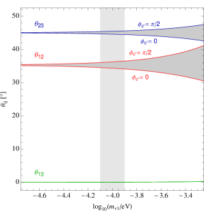
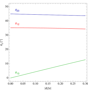
Figure 1: Numerical results using the MPT/REAP package [49] for the corrections to the lepton mixing angles in CSD (left panel) and PCSD (right panel), where in the latter case $c^{\prime}$ has been set to zero. In CSD (left panel), the NNLO correction depends on the mass of the lightest neutrino, $m_{\nu_{1}}$, and the light-grey vertical band shows the typical expectation for $m_{\nu_{1}}$ in some classes of GUT models. While $\theta_{13}$ is rather stable and remains close to zero, the deviation of $\theta_{12}$ from the tri-bimaximal value is about twice the deviation of $\theta_{23}$ from $\pi/4$. The two extreme cases with $\phi_{c^{\prime}}=0,\pi/2$ (note that the change of both, $\theta_{12}$ and $\theta_{23}$ is approximately proportional to $\cos(2\phi_{c^{\prime}})$) are displayed and the grey area between the curves corresponds to other values of $\phi_{c^{\prime}}$. In PCSD (right panel) with zero $c^{\prime}$, $\theta_{12}$ and $\theta_{23}$ are nearly unchanged and only $\theta_{13}$ increases with increasing $|d|/|e|=|d|/|f|$. The results agree well with the analytic results, and confirm that in the case of PCSD there there are small NLO corrections to $\theta_{23}$ and $\theta_{12}$ proportional to $\theta_{13}$ which are not seen in the analytic results.

6 Analytical vs. numerical results in two example models

In the previous section, analytic expressions of the mixing angles, involving NLO and NNLO corrections, were derived. Approximate results in the case of CSD and PCSD were also presented and the NLO corrections vanished in both cases. In this section, we evaluate the analytic results for two different numerical GUT inspired models. These are models of light sequential dominance (LSD) and heavy sequential dominance (HSD) [2, 7] previously studied in [44]. We also present numerical results for the neutrino masses, presented in Appendix B, as well as the difference in neutrino masses squared for both models.

6.1 Results for the LSD model

6.1.1 The CSD case

We consider a simple numerical example with a diagonal right-handed neutrino Majorana mass matrix $M_{RR}$ given by,

$$M_{RR}=\left(\begin{array}[]{ccc}5.1\times 10^{-9}&0&0\\ 0&7.05\times 10^{-9}&0\\ 0&0&1\end{array}\right)M_{3},$$ (6.1)

where $M_{3}=10^{16}GeV$. We also consider a neutrino Yukawa matrix of the form,

$$Y^{\nu}_{LR}=\left(\begin{array}[]{ccc}0&a&0\\ e&b&0\\ f&c&c^{\prime}\end{array}\right),$$ (6.2)

where we have taken the complex coupling $d$ to be zero. As required by CSD, we take $|a|=|b|=|c|=8.125\times 10^{-5}$ and $|e|=|f|=2.125\times 10^{-4}$. The value of the third family coupling $c^{\prime}$ is taken to be $|c^{\prime}|=0.5809$. We choose all the phases of the Yukawa couplings to be zero except $\phi_{e}$ ($\phi_{e}=\pi$).

Parameter	$|d|$	$|c^{\prime}|$	$\theta_{23}(\,^{\circ})$	$\theta_{13}(\,^{\circ})$	$\theta_{12}(\,^{\circ})$	$m_{1}$ (eV)	$m_{2}$ (eV)	$m_{3}$ (eV)
Analytic	$0$	$0.5809$	44.44	0.04	33.75	$1.52\times 10^{-4}$	$8.8\times 10^{-3}$	$0.055$
MPT/REAP	$0$	$0.5809$	44.38	0.05	33.69	$1.61\times 10^{-4}$	$8.8\times 10^{-3}$	$0.054$

Table 1: Analytical vs. numerical results for the mixing angles and masses, evaluated in the CSD case with $c^{\prime}\not=0$, for a model with light sequential dominance.

Numerical results for the mixing angles, evaluated in CSD using the analytic formulae, are presented in Tab. 1. This table also shows numerical results obtained using MPT/REAP package [49], which appear to be very close to the ones obtained through the analytic approach. We note that here and in the remainder of the paper, the MPT/REAP results were evaluated using the MPT package without considering RG running. As can be seen from Tab. 1, all the values of the mixing angles are slightly deviated from their TB values and this is mainly due to the presence of the non-zero 3-3 Yukawa coupling $c^{\prime}$. In addition, we present numerical results for the neutrino masses $m_{1},m_{2}$ and $m_{3}$ given by Eqs. (B.13), (B.14), (B.15), using both MPT/REAP and the analytic formulae. As presented in Tab. 1, we can see that the MPT/REAP and the analytic results are very close particularly in the case of $m_{2}$.

6.1.2 The PCSD case

We consider the previous LSD model in the case of PCSD with non-zero Yukawa coupling $d=0.2|e|$, $|e|=2.125\times 10^{-4}$ and $|c^{\prime}|=0$. Keeping all the other conditions of CSD satisfied as outlined in Section 6.1.1, we found that the numerical values of all the mixing angles are deviated from their TB values particularly the reactor angle $\theta_{13}$ which becomes larger than zero and takes a value of $8.22^{\circ}$ as shown in Tab. 2. This large value satisfies the predictions of TBR mixing and it is in good agreement with the most recent experimental results [40].

MPT/REAP results for the neutrino mixing angles in this case are slightly different than the analytic results as presented in Tab. 2. This is mainly due to the approximate nature of the diagonalisation procedure that we followed in this paper. Tab. 2 also shows numerical results for the neutrino masses $m_{1},m_{2}$ and $m_{3}$ evaluated in PCSD using both MPT/REAP and the analytic expressions. As expected, the neutrino mass $m_{1}$ is exactly zero in this case due to the vanishing NNLO corrections. We note that the results for the masses $m_{2},m_{3}$ in the analytic case are slightly different than the MPT/REAP case. This is also due to the difference in the diagonalisation approaches considered in the two cases.

Parameter	$|d|$	$|c^{\prime}|$	$\theta_{23}(\,^{\circ})$	$\theta_{13}(\,^{\circ})$	$\theta_{12}(\,^{\circ})$	$m_{1}$ (eV)	$m_{2}$ (eV)	$m_{3}$ (eV)
Analytic	$0.2|e|$	$0$	45.00	8.10	35.08	$0$	$8.5\times 10^{-3}$	$5.38\times 10^{-2}$
MPT/REAP	$0.2|e|$	$0$	44.29	8.53	34.89	0	$8.4\times 10^{-3}$	$5.4\times 10^{-2}$

Table 2: Analytical vs. numerical results for the neutrino mixing angles and masses, evaluated in the PCSD case for a model with light sequential dominance, with $c^{\prime}=0$ and $|d|=0.2|e|$.

In order to compare our numerical values to experimental data, we present numerical results for the difference in the squares of neutrino masses $\Delta m^{2}_{sol}$ and $\Delta m^{2}_{atm}$, evaluated for the LSD model in CSD and PCSD, as shown in Tab. 3. These results are evaluated at the SD cases using both the analytic results as well as MPT/REAP. The numerical results, as shown in Tab. 3, are within the most recent experimental ranges presented in [40] particularly for the value of $\Delta m^{2}_{sol}$ in CSD which is very close to the best fit value of $7.6\times 10^{-5}eV^{2}$.

Parameter	Analytic	MPT/REAP	Analytic	MPT/REAP
SD limit	CSD	CSD	PCSD	PCSD
$\Delta m^{2}_{sol}$ ($eV^{2}$)	$7.5\times 10^{-5}$	$7.5\times 10^{-5}$	$7.3\times 10^{-5}$	$7.1\times 10^{-5}$
$\Delta m^{2}_{atm}$ ($eV^{2}$)	$2.11\times 10^{-3}$	$2.04\times 10^{-3}$	$2.05\times 10^{-3}$	$2.1\times 10^{-3}$

Table 3: Analytical vs. numerical results of the difference in the squares of neutrino masses ($\Delta m^{2}_{sol}$ and $\Delta m^{2}_{atm}$) evaluated for the LSD model. The results are presented at CSD with non-zero $c^{\prime}$ as well as the PCSD case with zero $c^{\prime}$ and non- zero coupling $|d|=0.2|e|$.

6.2 Results for the HSD model

To check the generality of our numerical results, we consider another model with heavy sequential dominance (HSD). The right-handed neutrino Majorana mass matrix $M_{RR}$, in this case, is given by,

$$M_{RR}=\left(\begin{array}[]{ccc}3.991\times 10^{8}&0&0\\ 0&5.8\times 10^{10}&0\\ 0&0&5.021\times 10^{14}\end{array}\right).$$ (6.3)

This model satisfies HSD where the dominant contribution to the neutrino mass is coming from the heaviest right-handed neutrino. The neutrino Yukawa matrix is of the form given in Eq. (6.2) with the following values of the Yukawa couplings: $|a|=|b|=|c|=2.401\times 10^{-3}$, $|e|=|f|=0.677$ and $|c^{\prime}|=2.992\times 10^{-5}$. Similarly to the LSD model, we take all the phases of the Yukawa couplings to be zero except the coupling $e$ ($\phi_{e}=\pi$).

Analytic and MPT/REAP results of the mixing angles and masses, in CSD, are presented and compared as shown in Tab. 4. We note that, for this model, the values of the mixing angles are much closer to their TB values compared to the LSD model, which is mainly due to the smallness of the 3-3 Yukawa coupling $c^{\prime}$ in this case. We also present results for the PCSD case with non-zero 1-1 Yukawa coupling ($d$), as shown in Tab. 5. Analogously to the LSD model, the reactor angle for the HSD model, is found to be large and within the recent experimental range presented in [40]. The neutrino mass $m_{1}$ is exactly zero at the PCSD case with $c^{\prime}=0$ as expected.

Parameter	$|d|$	$|c^{\prime}|$	$\theta_{23}(\,^{\circ})$	$\theta_{13}(\,^{\circ})$	$\theta_{12}(\,^{\circ})$	$m_{1}$ (eV)	$m_{2}$ (eV)	$m_{3}$ (eV)
Analytic	$0$	$2.99\times 10^{-5}$	44.96	$0.003$	35.18	$1.01\times 10^{-5}$	$9\times 10^{-3}$	$0.055$
MPT/REAP	$0$	$2.99\times 10^{-5}$	44.96	$0.003$	35.16	$1.1\times 10^{-5}$	$9\times 10^{-3}$	$0.055$

Table 4: Analytical vs. numerical results for the neutrino mixing angles and masses, evaluated in CSD with $c^{\prime}\not=0$, for a model with heavy sequential dominance.

Parameter	$|d|$	$|c^{\prime}|$	$\theta_{23}(\,^{\circ})$	$\theta_{13}(\,^{\circ})$	$\theta_{12}(\,^{\circ})$	$m_{1}$ (eV)	$m_{2}$ (eV)	$m_{3}$ (eV)
Analytic	$0.2|e|$	$0$	45.00	$8.10$	35.08	$0$	$9\times 10^{-3}$	$0.055$
MPT/REAP	$0.2|e|$	$0$	$44.27$	$8.55$	$34.89$	$0$	$8.9\times 10^{-3}$	$0.056$

Table 5: Analytical vs. numerical results for the neutrino mixing angles and masses, evaluated in the PCSD case for a model with heavy sequential dominance, with $c^{\prime}=0$ and $|d|=0.2|e|$.

Similarly to the LSD model, we present numerical results for the difference in the squares of neutrino masses $\Delta m^{2}_{sol}$ and $\Delta m^{2}_{atm}$, evaluated for the HSD model, as shown in Tab. 6. The results for this model, which are also presented at both SD cases using analytic results as well as MPT/REAP, are within the most recent experimental ranges presented in [40]. We note that the values of $\Delta m^{2}_{sol}$, in all cases presented in Tab. 6, are closer to the upper limit of the $3\sigma$ experimental range [40].

Parameter	Analytic	MPT/REAP	Analytic	MPT/REAP
SD limit	CSD	CSD	PCSD	PCSD
$\Delta m^{2}_{sol}$ ($eV^{2}$)	$8.2\times 10^{-5}$	$8.15\times 10^{-5}$	$8.2\times 10^{-5}$	$8\times 10^{-5}$
$\Delta m^{2}_{atm}$ ($eV^{2}$)	$2.16\times 10^{-3}$	$2.13\times 10^{-3}$	$2.16\times 10^{-3}$	$2.2\times 10^{-3}$

Table 6: Analytical vs. numerical results of the difference in the squares of neutrino masses ($\Delta m^{2}_{sol}$ and $\Delta m^{2}_{atm}$) evaluated for the HSD model. The results are presented at CSD with non-zero $c^{\prime}$ as well as the PCSD case with zero $c^{\prime}$ and non- zero coupling $|d|=0.2|e|$.

To summarize, the comparison between the analytical results and the numerical values using MPT/REAP has shown small differences, which are however within the expected range due to the approximate nature of the diagonalisation procedure followed in this paper. Explicitly, $\theta_{12}$ from the analytical results has been larger by about $0.2^{\circ}$ than the MPT/REAP value, $\theta_{23}$ is larger by $0.7^{\circ}$ while the reactor angle $\theta_{13}$ is smaller by about $0.4^{\circ}$ than the MPT/REAP value for both models. We have also presented numerical results for the neutrino masses as well as the difference in the squares of neutrino masses ($\Delta m^{2}_{sol}$ and $\Delta m^{2}_{atm}$), in the SD cases, using MPT/REAP and the analytic formulae. The numerical results for $\Delta m^{2}_{sol}$ and $\Delta m^{2}_{atm}$ are within the most recent experimental ranges [40].

7 Summary and Conclusions

SD provides a natural way of having large mixing angles together with hierarchical neutrino masses from the type I see-saw mechanism. In this paper we have derived analytic expressions for the neutrino mixing angles including the NLO and NNLO corrections arising from the second lightest and lightest neutrino masses. We have pointed out that for special cases of SD corresponding to form dominance the NLO and NNLO corrections both vanish. This observation helps to explain why the LO results for SD are sometimes observed to work better than expected in particular cases. For example, we have studied tri-bimaximal mixing via constrained sequential dominance which involves only a NNLO correction as an example of softly broken FD where the corrections vanish in the strong hierarchical limit. We have also considered tri-bimaximal-reactor mixing via partially constrained sequential dominance and shown that this involves NLO corrections to neutrino mixing angles suppressed by the small reactor angle which renders such corrections negligible. This supports the PCSD proposal as a robust way of obtaining a significant non-zero reactor angle with the atmospheric and solar angles remaining close to their tri-bimaximal values to an accuracy of a few per cent.

We have evaluated these analytic results for two explicit GUT inspired models of so-called LSD type and HSD type including, in the case of CSD, the deviations from exact TB mixing due to the presence of a non-zero third family Yukawa coupling. For both models the analytic results agree well with the numerical results obtained from extracting the mixing angles using the MPT tool provided with MPT/REAP. In the CSD case the absence of NLO corrections is confirmed numerically while the soft NNLO corrections are observed. We have also seen that the analytic expressions in the case of PCSD with zero third family Yukawa coupling involves no NLO corrections in the approximation that NLO corrections multiplied by the reactor angle are dropped. The numerical results for PCSD confirm that the atmospheric and solar angles remain very close to their TB values while the reactor angle, $\theta_{13}$, is much larger than zero, and confirm that the NLO corrections are suppressed by the reactor angle. If a sizeable reactor angle is measured it may therefore be possible to retain the tri-bimaximal predictions for the atmospheric and solar angles to a few per cent accuracy using PCSD. We note, however, that this neglects other model dependent charged lepton, RG and canonical normalization corrections which have been considered elsewhere.

To conclude, we have derived approximate analytic results which allow to extract the neutrino mixing angles in the framework of see-saw mechanism with sequential dominance including NLO and NNLO corrections from $m_{2}$ and $m_{1}$. We have shown that, for the special case of FD, the NLO and NNLO corrections vanish. CSD is an example where FD is only violated softly leading to NNLO corrections only, a result supported by numerical evaluation. Such NNLO corrections are typical in many classes of GUT models with hierarchical Yukawa matrices which lead to LSD with $m_{1}$ arising from the large third family Yukawa coupling. We emphasise that in realistic models, FD and CSD are enforced by family symmetry and so in testing these schemes one is really testing particular models based on family symmetry. It is possible for FD to yield either a normal mass ordering or an inverted one, while CSD always corresponds to a normal mass hierarchy. We have also shown that, in the case of PCSD, the NLO corrections are suppressed by the reactor angle, and have again verified this result numerically. In other special cases of SD which are close to the FD limit, one can similarly expect the NLO and NNLO corrections to neutrino mixing angles to be suppressed. However, if significant deviations from TB mixing are observed, then the more general cases of SD away from the FD limit, as considered in this paper, would become relevant. The analytic results for neutrino mixing angles in SD presented here, including the NLO and NNLO corrections, are therefore applicable to a wider class of models and may be reliably used when confronting such models with high precision neutrino data, providing useful insights beyond a purely numerical analysis.

Appendix A Diagonalisation of left-handed neutrino matrix

In this Appendix, we will briefly review the procedure of diagonalising the neutrino mass matrix following [5] closely. We start by writing the left-handed neutrino mass matrix as,

$$m_{LL}^{\nu}=\left(\begin{array}[]{ccc}m_{11}&m_{12}&m_{13}\\ m_{12}&m_{22}&m_{23}\\ m_{13}&m_{23}&m_{33}\end{array}\right)\equiv\left(\begin{array}[]{ccc}|m_{11}|e^{i\phi_{11}}&|m_{12}|e^{i\phi_{12}}&|m_{13}|e^{i\phi_{13}}\\ |m_{12}|e^{i\phi_{12}}&|m_{22}|e^{i\phi_{22}}&|m_{23}|e^{i\phi_{23}}\\ |m_{13}|e^{i\phi_{13}}&|m_{23}|e^{i\phi_{23}}&|m_{33}|e^{i\phi_{33}}\end{array}\right)$$ (A.1)

In general, we diagonalise a complex, hierarchical, neutrino matrix by following a sequence of transformations [5],

$${P_{3}^{\nu_{L}}}^{*}{R_{12}}^{T}{P_{1}^{\nu_{L}}}^{*}{R_{13}^{\nu_{L}}}^{T}{R_{23}^{\nu_{L}}}^{T}{P_{2}^{\nu_{L}}}^{*}m_{LL}^{\nu}P_{2}^{\nu_{L}}R_{23}^{\nu_{L}}R_{13}^{\nu_{L}}P_{1}^{\nu_{L}}R_{12}^{\nu_{L}}P_{3}^{\nu_{L}}=\left(\begin{array}[]{ccc}m_{1}&0&0\\ 0&m_{2}&0\\ 0&0&m_{3}\end{array}\right),$$ (A.2)

where the resulting matrix includes the three different neutrino masses $m_{1},m_{2}$ and $m_{3}$. $R_{ij},~{}i,j=\{1,2,3\}$ are a set of real rotations, involving the Euler angles $\theta_{ij}$, which can be written as,

$$R_{23} = \left(\begin{array}[]{ccc}1&0&0\\ 0&c_{23}&s_{23}\\ 0&-s_{23}&c_{23}\\ \end{array}\right)$$ (A.6)

$$R_{13} = \left(\begin{array}[]{ccc}c_{13}&0&s_{13}\\ 0&1&0\\ -s_{13}&0&c_{13}\\ \end{array}\right)$$ (A.10)

$$R_{12} = \left(\begin{array}[]{ccc}c_{12}&s_{12}&0\\ -s_{12}&c_{12}&0\\ 0&0&1\\ \end{array}\right).$$ (A.14)

The matrices $P_{i}$ in Eq. (A.2) are the phase matrices, involving the phases $\phi_{2},\phi_{3},\chi$ and $\omega_{i}$, which we write as,

$$P_{1} = \left(\begin{array}[]{ccc}1&0&0\\ 0&e^{i\chi}&0\\ 0&0&1\\ \end{array}\right)$$ (A.18)

$$P_{2} = \left(\begin{array}[]{ccc}1&0&0\\ 0&e^{i\phi_{2}}&0\\ 0&0&e^{i\phi_{3}}\\ \end{array}\right)$$ (A.22)

$$P_{3} = \left(\begin{array}[]{ccc}e^{i\omega_{1}}&0&0\\ 0&e^{i\omega_{2}}&0\\ 0&0&e^{i\omega_{3}}\\ \end{array}\right)$$ (A.26)

We briefly summarise the different steps of diagonalisation following [5]. We start by multiplying the mass matrix, given by Eq. (A.1), by the inner complex phase matrices $P_{2}$, which helps in performing the diagonalisation procedure. This process modifies the phases of the matrix as follows,

$$m_{LL}=\left(\begin{array}[]{ccc}|m_{11}|e^{i\phi_{11}}&|m_{12}|e^{i(\phi_{12}-\phi_{2})}&|m_{13}|e^{i(\phi_{13}-\phi_{3})}\\ |m_{12}|e^{i(\phi_{12}-\phi_{2})}&|m_{22}|e^{i(\phi_{22}-2\phi_{2})}&|m_{23}|e^{i(\phi_{23}-\phi_{2}-\phi_{3})}\\ |m_{13}|e^{i(\phi_{13}-\phi_{3})}&|m_{23}|e^{i(\phi_{23}-\phi_{2}-\phi_{3})}&|m_{33}|e^{i(\phi_{33}-2\phi_{3})}\end{array}\right)$$ (A.27)

After re-phasing the matrix, we proceed by applying the real rotation $R_{23}$, defined in Eq. (A.6). This step modifies the lower 23 block of the mass matrix by putting zeroes in the 23, 32 elements of the matrix [5],

$$\left(\begin{array}[]{cc}\tilde{m}_{22}&0\\ 0&m_{3}^{\prime}\end{array}\right)\equiv{R^{\nu_{L}}_{23}}^{T}\left(\begin{array}[]{cc}|m_{22}|e^{i(\phi_{22}-2\phi_{2})}&|m_{23}|e^{i(\phi_{23}-\phi_{2}-\phi_{3})}\\ |m_{23}|e^{i(\phi_{23}-\phi_{2}-\phi_{3})}&|m_{33}|e^{i(\phi_{33}-2\phi_{3})}\end{array}\right)R^{\nu_{L}}_{23}$$ (A.28)

This diagonalisation not only modifies the masses $m_{22}$ and $m_{33}$ but also all the other mass entries except $m_{11}$. Substituting for these masses in terms of the Yukawa couplings, we get an analytic formula for $\tan(\theta_{23})$. The phases $\phi_{2},\phi_{3}$, appearing in Eqs.(A.27,A.28), are fixed in order to have real $\tan(\theta_{23})$. The next step, as shown in Eq. (A.2), is to apply the rotation $R_{13}$ which diagonalises the outer 13 block. Similar to the previous step, this rotation modifies the matrix by putting zeros in the 13, 31 entries.

After applying the 13 rotation, the neutrino mass matrix can be written as,

$${R_{13}^{\nu_{L}}}^{T}{R_{23}^{\nu_{L}}}^{T}{P_{2}^{\nu_{L}}}^{*}m_{LL}P_{2}^{\nu_{L}}R_{23}^{\nu_{L}}R_{13}^{\nu_{L}}=\left(\begin{array}[]{ccc}\tilde{m}_{11}&\tilde{m}_{12}&0\\ \tilde{m}_{12}&\tilde{m}_{22}&0\\ 0&0&m^{\prime}_{3}\end{array}\right)$$ (A.29)

The last step of the diagonalisation involves modifying the upper 12 block of the matrix. To do this, we first multiply the result of the last step by the phase matrix ${P_{1}}$, which introduces the phase $\chi$. We then apply the real rotation $R_{12}$. The neutrino mass matrix can then be written as follows,

$${R^{\nu}_{12}}^{T}\left(\begin{array}[]{ccc}\tilde{m}_{11}&\tilde{m}^{\prime}_{12}&0\\ \tilde{m}^{\prime}_{12}&\tilde{m}^{\prime}_{22}&0\\ 0&0&m^{\prime}_{3}\end{array}\right)R^{\nu}_{12}=\left(\begin{array}[]{ccc}m^{\prime}_{1}&0&0\\ 0&m^{\prime}_{2}&0\\ 0&0&m^{\prime}_{3}\end{array}\right),$$ (A.30)

where the new masses $\tilde{m}^{\prime}_{12},\tilde{m}^{\prime}_{22}$ are written as,

$$\tilde{m}^{\prime}_{12}=\tilde{m}_{12}~{}e^{i\chi},~{}~{}\tilde{m}^{\prime}_{22}=\tilde{m}_{22}~{}e^{i2\chi}.$$

From Eq. (A.30), we can see that the neutrino matrix is successfully diagonalised, however, we still need to multiply the result by the phase matrix $P_{3}$ in order to make all the diagonal elements real. To proceed, we write the resulting mass matrix by substituting for the diagonal mass terms as $m^{\prime}_{i}\equiv m_{i}e^{i\phi^{\prime}_{i}},~{}i=\{1,2,3\}$. We then apply the phase matrix and write the phases $\omega_{i}$ as $\omega_{i}=\phi^{\prime}_{i}/2$. These phases cancel with the phases of the neutrino mass matrix which gives a real, diagonal, neutrino matrix as required.

Appendix B Derivation of mass terms

In this Appendix, we present the derivations of the mass terms resulting from the diagonalisation of the mass matrix. After applying the rotation $R_{23}$ (c.f. Eq. (A.6)), we can derive expressions for the masses $m^{\prime}_{3}$ and $\tilde{m}_{22}$ which are necessary for deriving expressions for $\theta_{13}$ and $\tan(\theta_{12})$. To find these masses, we first take the trace of both sides of Eq. (A.28) which gives,

$$\tilde{m}_{22}+m^{\prime}_{3} \approx m_{22}e^{-i2\phi_{2}}+m_{33}e^{-i2\phi_{3}}$$ (B.1)

$$\approx e^{i(2\phi_{e}-2\phi_{2})}\frac{|e|^{2}+|f|^{2}}{Y}\left(1+\epsilon_{3}(s^{0}_{23})^{2}+(c^{0}_{23})^{2}(\epsilon_{2}+\eta_{1})\right),$$

We can also express the determinant of both sides of Eq. (A.28). This reads,

$$\tilde{m}_{22}m^{\prime}_{3} = m_{22}e^{-2i\phi_{2}}m_{33}e^{-2i\phi_{3}}-(m_{23})^{2}e^{-2i(\phi_{2}+\phi_{3})}$$ (B.2)

$$= e^{-2i(\phi_{2}+\phi_{3})}\left(\frac{c^{\prime 2}}{X^{\prime}}(\frac{b^{2}}{X}+\frac{e^{2}}{Y})+\frac{(bf-ec)^{2}}{XY}\right)$$

We take the mass term $m^{\prime}_{3}$ to have the following form,

$$m^{\prime}_{3}\approx m^{\prime 0}_{3}(1+\beta),$$ (B.3)

where the parameter $\beta$ is given by Eq. (4.6) and the mass term $m^{\prime 0}_{3}\equiv m^{\prime}_{3}|_{\epsilon_{i}=0,\eta_{i}=0}$ is given by,

$$m^{\prime 0}_{3}\approx e^{i(2\phi_{e}-2\phi_{2})}\frac{|e|^{2}+|f|^{2}}{Y},$$ (B.4)

Using Eqs.(B.1), (B.2), (B.4), $\tilde{m}_{22}$ can be written as,

$$\tilde{m}_{22}\approx\left(\tilde{m}_{22}^{0}+\eta_{2}\left(\frac{b^{2}}{X}+\frac{e^{2}}{Y}\right)\right)(1-\beta),$$ (B.5)

where

$$\tilde{m}_{22}^{0}\equiv\tilde{m}_{22}|_{c^{\prime}=0,\epsilon_{i}=0}\approx e^{-2i\phi_{2}}\frac{(bc_{23}^{0}-cs_{23}^{0}e^{i(\phi_{e}-\phi_{f})})^{2}}{X},$$ (B.6)

and the parameter $\eta_{2}$ is given by Eq. (4.16).

In addition to the derivation of the masses $\tilde{m}_{22},m^{\prime}_{3}$, applying the rotation $R_{23}$, modifies the masses $m_{12},m_{13}$. These become $\tilde{m}_{12},\tilde{m}_{13}$, after diagonalising the 23 block, and can be derived to leading order as follows

$$\tilde{m}_{12} = c_{23}m_{12}e^{-i\phi_{2}}-s_{23}m_{13}e^{-i\phi_{3}},$$ (B.7)

$$\approx \tilde{m}_{12}^{0}(1-\gamma(s_{23}^{0})^{2})-e^{-i\phi_{3}}\gamma s_{23}^{0}(\frac{ac}{X}+\frac{df}{Y}),$$

$$\tilde{m}_{13} = s_{23}m_{12}e^{-i\phi_{2}}+c_{23}m_{13}e^{-i\phi_{3}}$$ (B.8)

$$\approx \tilde{m}_{13}^{0}(1-\gamma(s_{23}^{0})^{2})+e^{-i\phi_{2}}\gamma s_{23}^{0}(\frac{ab}{X}+\frac{de}{Y}),$$

where the parameter $\gamma$ is given by Eq. (4.4), the masses $\tilde{m}_{12}^{0}\equiv\tilde{m}_{12}|_{c^{\prime}=0,\epsilon_{i}=0}$ and $\tilde{m}_{13}^{0}\equiv\tilde{m}_{13}|_{c^{\prime}=0,\epsilon_{i}=0}$ are given to leading order, as presented in [5], by

$$\tilde{m}_{12}^{0} \approx e^{-i\phi_{2}}\frac{a(c_{23}^{0}b-s_{23}^{0}ce^{i(\phi_{e}-\phi_{f})})}{X},$$ (B.9)

$$\tilde{m}_{13}^{0} \approx e^{-i\phi_{2}}\left(\frac{a}{X}(s^{0}_{23}b+c^{0}_{23}ce^{i(\phi_{e}-\phi_{f})})+e^{i\phi_{e}}\frac{d\sqrt{|e|^{2}+|f|^{2}}}{Y}\right).$$ (B.10)

After applying the $R_{13}$ rotation, we obtain another mass term, $\tilde{m}_{11}$, which can be presented to leading order as

$$\tilde{m}_{11} \approx m_{11}-\frac{\tilde{m}_{13}^{2}}{m^{\prime}_{3}}$$ (B.11)

$$\approx \tilde{m}^{0}_{11}(1-2\gamma(s^{0}_{23})^{2}-\beta)+\frac{a^{2}}{X}(2\gamma(s^{0}_{23})^{2}+\beta)+\frac{d^{2}}{Y}(2\gamma(s^{0}_{23})^{2}+\beta)$$

$$- 2e^{-2i\phi_{e}}\epsilon_{6}(s^{0}_{23}b+c^{0}_{23}ce^{i(\phi_{e}-\phi_{f})})\gamma s^{0}_{23}\left(\frac{ab}{X}+\frac{de}{Y}\right)$$

where the leading order form of $\tilde{m}^{0}_{11}\equiv\tilde{m}_{11}|_{\eta_{i}=0,\epsilon_{i}=0}$ is given in [5],

$${m}^{0}_{11}\approx\frac{a^{2}}{X}-e^{-i\phi_{e}}\frac{2d}{\sqrt{|e|^{2}+|f|^{2}}}\frac{a(s^{0}_{23}b+c^{0}_{23}ce^{i(\phi_{e}-\phi_{f})})}{X},$$ (B.12)

The small parameter $\epsilon_{6}$ is written as,

$$\epsilon_{6}=\frac{a}{X}\left(\frac{|e|^{2}+|f|^{2}}{Y}\right)^{-1}.$$

Similar to the derivation of the masses $\tilde{m}_{22},m^{\prime}_{3}$, the neutrino masses $m^{\prime}_{1}$ and $m^{\prime}_{2}$ can be written using the trace and the determinant of the upper 12 block of Eq. (A.30). The real neutrino masses $m_{1},m_{2}$ can then be written, in the SD cases, as

$$m_{1} \approx \frac{|c^{\prime}|^{2}}{6X^{\prime}}\left(1-\frac{Y}{X}\frac{|b|^{2}}{|e|^{2}}+\frac{2|d|}{|e|}\right),$$ (B.13)

$$m_{2} \approx \left(\frac{3|b|^{2}}{X}+\frac{|c^{\prime}|^{2}}{3X^{\prime}}\left(1-\frac{Y}{X}\frac{|b|^{2}}{|e|^{2}}-\frac{|d|}{|e|}\right)\cos(2\phi_{c^{\prime}})\right),$$ (B.14)

The neutrino mass $m_{3}$ can be written in the SD cases, using Eqs.(B.3), (B.4), as

$$m_{3}\approx\left(\frac{2|e|^{2}}{Y}+\frac{|c^{\prime}|^{2}}{X^{\prime}}\cos(2\phi_{c^{\prime}})\right).$$ (B.15)

References

- [1] P. Minkowski, Phys. Lett. B 67 (1977) 421; M. Gell-Mann, P. Ramond and R. Slansky in Sanibel Talk, CALT-68-709, Feb 1979, and in Supergravity (North Holland, Amsterdam 1979); T. Yanagida in Proc. of the Workshop on Unified Theory and Baryon Number of the Universe, KEK, Japan, 1979; S.L.Glashow, Cargese Lectures (1979); R. N. Mohapatra and G. Senjanovic, Phys. Rev. Lett. 44 (1980) 912; J. Schechter and J. W. Valle, Phys. Rev. D 25 (1982) 774.
- [2] S. F. King, Phys. Lett. B 439 (1998) 350 [arXiv:hep-ph/9806440]; S. F. King, Nucl. Phys. B 562 (1999) 57 [arXiv:hep-ph/9904210]; G. Altarelli, F. Feruglio and I. Masina, Phys. Lett. B 472 (2000) 382 [arXiv:hep-ph/9907532].
- [3] S. F. King, Nucl. Phys. B 576 (2000) 85 [arXiv:hep-ph/9912492].
- [4] S. Lavignac, I. Masina and C. A. Savoy, Nucl. Phys. B 633 (2002) 139 [arXiv:hep-ph/0202086].
- [5] S. F. King, JHEP 0209 (2002) 011 [arXiv:hep-ph/0204360].
- [6] S. F. King, Phys. Rev. D 67 (2003) 113010 [arXiv:hep-ph/0211228].
- [7] For a review of sequential dominance, see: S. Antusch and S. F. King, New J. Phys. 6 (2004) 110 [arXiv:hep-ph/0405272];
- [8] N. Haba, R. Takahashi, M. Tanimoto and K. Yoshioka, Phys. Rev. D 78 (2008) 113002 [arXiv:0804.4055 [hep-ph]].
- [9] A. Bandyopadhyay et al. [ISS Physics Working Group], Rept. Prog. Phys. 72 (2009) 106201 [arXiv:0710.4947 [hep-ph]].
- [10] M. C. Chen and S. F. King, arXiv:0903.0125 [hep-ph].
- [11] S. Antusch, L. E. Ibanez and T. Macri, JHEP 0709 (2007) 087 [arXiv:0706.2132 [hep-ph]].
- [12] S. F. King, JHEP 0508 (2005) 105 [arXiv:hep-ph/0506297].
- [13] P. F. Harrison, D. H. Perkins and W. G. Scott, Phys. Lett. B 530 (2002) 167 [arXiv:hep-ph/0202074]; P. F. Harrison and W. G. Scott, Phys. Lett. B 535 (2002) 163 [arXiv:hep-ph/0203209]; P. F. Harrison and W. G. Scott, Phys. Lett. B 557 (2003) 76 [arXiv:hep-ph/0302025]; see also L. Wolfenstein, Phys. Rev. D 18 (1978) 958.
-
[14]
C. S. Lam,
Phys. Lett. B 656 (2007) 193 [arXiv:0708.3665];
C. S. Lam, Phys. Rev. Lett. 101 (2008) 121602 [arXiv:0804.2622];
C. S. Lam, Phys. Rev. D 78 (2008) 073015 [arXiv:0809.1185]. - [15] S. F. King and C. Luhn, JHEP 0910 (2009) 093 [arXiv:0908.1897 [hep-ph]].
-
[16]
W. Grimus and L. Lavoura,
JHEP 0508 (2005) 013 [hep-ph/0504153];
W. Grimus and L. Lavoura, JHEP 0601 (2006) 018 [hep-ph/0509239];
R. N. Mohapatra, S. Nasri and H. B. Yu, Phys. Lett. B 639 (2006) 318 [hep-ph/0605020];
Y. Koide, Eur. Phys. J. C 50 (2007) 809 [hep-ph/0612058];
M. Mitra and S. Choubey, Phys. Rev. D 78 (2008) 115014 [arXiv:0806.3254]. -
[17]
W. Grimus and L. Lavoura,
Phys. Lett. B 572 (2003) 189
[hep-ph/0305046];
A. Adulpravitchai, A. Blum and C. Hagedorn, JHEP 0903 (2009) 046 [arXiv:0812.3799]; H. Ishimori, T. Kobayashi, H. Ohki, Y. Omura, R. Takahashi and M. Tanimoto, Phys. Lett. B 662 (2008) 178 [arXiv:0802.2310 [hep-ph]]; H. Ishimori, T. Kobayashi, H. Ohki, Y. Omura, R. Takahashi and M. Tanimoto, Phys. Rev. D 77 (2008) 115005 [arXiv:0803.0796 [hep-ph]]. -
[18]
E. Ma and G. Rajasekaran,
Phys. Rev. D 64 (2001) 113012 [hep-ph/0106291];
E. Ma, Phys. Rev. D 73 (2006) 057304 [hep-ph/0511133];
G. Altarelli and F. Feruglio, Nucl. Phys. B 720 (2005) 64 [hep-ph/0504165];
K. S. Babu and X. G. He, hep-ph/0507217;
G. Altarelli and F. Feruglio, Nucl. Phys. B 741 (2006) 215 [hep-ph/0512103];
G. Altarelli, F. Feruglio and Y. Lin, Nucl. Phys. B 775 (2007) 31 [hep-ph/0610165];
M. Hirsch, A. S. Joshipura, S. Kaneko and J. W. F. Valle, Phys. Rev. Lett. 99 (2007) 151802 [hep-ph/0703046];
M. Honda and M. Tanimoto, Prog. Theor. Phys. 119 (2008) 583 [arXiv:0801.0181];
Y. Lin, Nucl. Phys. B 813 (2009) 91 [arXiv:0804.2867];
M. C. Chen and S. F. King, JHEP 0906 (2009) 072 [arXiv:0903.0125];
G. Altarelli and D. Meloni, J. Phys. G 36 (2009) 085005 [arXiv:0905.0620]. - [19] Y. Koide, JHEP 0708 (2007) 086 [arXiv:0705.2275].
- [20] H. Ishimori, T. Kobayashi, H. Okada, Y. Shimizu and M. Tanimoto, JHEP 0904 (2009) 011 [arXiv:0811.4683].
-
[21]
J. Kubo, A. Mondragon, M. Mondragon and E. Rodriguez-Jauregui,
Prog. Theor. Phys. 109 (2003) 795,
Erratum-ibid. 114 (2005) 287 [hep-ph/0302196];
S. L. Chen, M. Frigerio and E. Ma, Phys. Rev. D 70 (2004) 073008 [Erratum-ibid. D 70 (2004) 079905] [hep-ph/0404084];
F. Feruglio and Y. Lin, Nucl. Phys. B 800 (2008) 77 [arXiv:0712.1528]. -
[22]
A. Blum, C. Hagedorn and M. Lindner,
Phys. Rev. D 77 (2008) 076004 [arXiv:0709.3450];
A. Blum, C. Hagedorn and A. Hohenegger, JHEP 0803 (2008) 070 [arXiv:0710.5061];
A. Blum and C. Hagedorn, Nucl. Phys. B 821 (2009) 327 [arXiv:0902.4885]. -
[23]
M. Frigerio, S. Kaneko, E. Ma and M. Tanimoto,
Phys. Rev. D 71 (2005) 011901 [hep-ph/0409187];
K. S. Babu and J. Kubo, Phys. Rev. D 71 (2005) 056006 [hep-ph/0411226];
Y. Kajiyama, E. Itou and J. Kubo, Nucl. Phys. B 743 (2006) 74 [hep-ph/0511268]. -
[24]
K. S. Babu, E. Ma and J. W. F. Valle,
Phys. Lett. B 552 (2003) 207 [hep-ph/0206292];
F. Bazzocchi, S. Morisi and M. Picariello, Phys. Lett. B 659 (2008) 628 [arXiv:0710.2928]. - [25] S. F. King and M. Malinsky, Phys. Lett. B 645 (2007) 351 [hep-ph/0610250].
-
[26]
A. Aranda, C. D. Carone and R. F. Lebed,
Phys. Rev. D 62 (2000) 016009 [hep-ph/0002044];
F. Feruglio, C. Hagedorn, Y. Lin and L. Merlo, Nucl. Phys. B 775 (2007) 120 [hep-ph/0702194];
M. C. Chen and K. T. Mahanthappa, Phys. Lett. B 652 (2007) 34 [arXiv:0705.0714];
P. H. Frampton and T. W. Kephart, JHEP 0709 (2007) 110 [arXiv:0706.1186];
A. Aranda, Phys. Rev. D 76 (2007) 111301 [arXiv:0707.3661];
P. H. Frampton and S. Matsuzaki, Phys. Lett. B 679 (2009) 347 [arXiv:0902.1140]. -
[27]
C. Hagedorn, M. Lindner and R. N. Mohapatra,
JHEP 0606 (2006) 042 [hep-ph/0602244];
G. J. Ding, Nucl. Phys. B 827 (2010) 82 [arXiv:0909.2210];
D. Meloni, arXiv:0911.3591 [hep-ph]. - [28] F. Bazzocchi, L. Merlo and S. Morisi, Nucl. Phys. B 816 (2009) 204 [arXiv:0901.2086].
-
[29]
G. Altarelli, F. Feruglio and C. Hagedorn,
JHEP 0803 (2008) 052
[arXiv:0802.0090];
P. Ciafaloni, M. Picariello, E. Torrente-Lujan and A. Urbano, Phys. Rev. D 79 (2009) 116010 [arXiv:0901.2236];
T. J. Burrows and S. F. King, arXiv:0909.1433. -
[30]
S. Morisi, M. Picariello and E. Torrente-Lujan,
Phys. Rev. D 75 (2007) 075015 [hep-ph/0702034];
F. Bazzocchi, M. Frigerio and S. Morisi, Phys. Rev. D 78 (2008) 116018 [arXiv:0809.3573]. -
[31]
H. Ishimori, Y. Shimizu and M. Tanimoto,
Prog. Theor. Phys. 121 (2009) 769
[arXiv:0812.5031];
H. Ishimori, T. Kobayashi, H. Ohki, H. Okada, Y. Shimizu and M. Tanimoto, arXiv:1003.3552;
C. Hagedorn, S. F. King and C. Luhn, arXiv:1003.4249 [Unknown]. -
[32]
D. G. Lee and R. N. Mohapatra,
Phys. Lett. B 329 (1994) 463
[hep-ph/9403201];
R. N. Mohapatra, M. K. Parida and G. Rajasekaran, Phys. Rev. D 69 (2004) 053007 [hep-ph/0301234];
Y. Cai and H. B. Yu, Phys. Rev. D 74 (2006) 115005 [hep-ph/0608022];
M. K. Parida, Phys. Rev. D 78 (2008) 053004 [arXiv:0804.4571];
B. Dutta, Y. Mimura and R. N. Mohapatra, arXiv:0911.2242. -
[33]
S. F. King and C. Luhn,
Nucl. Phys. B 820 (2009) 269
[arXiv:0905.1686];
S. F. King and C. Luhn, Nucl. Phys. B 832 (2010) 414 [arXiv:0912.1344]. - [34] C. Luhn, S. Nasri and P. Ramond, Phys. Lett. B 652 (2007) 27 [arXiv:0706.2341].
- [35] C. Hagedorn, M. A. Schmidt and A. Y. Smirnov, Phys. Rev. D 79 (2009) 036002 [arXiv:0811.2955].
-
[36]
I. de Medeiros Varzielas, S. F. King and G. G. Ross,
Phys. Lett. B 644 (2007) 153
[hep-ph/0512313];
I. de Medeiros Varzielas, S. F. King and G. G. Ross, Phys. Lett. B 648 (2007) 201 [hep-ph/0607045];
F. Bazzocchi and I. de Medeiros Varzielas, Phys. Rev. D 79 (2009) 093001 [arXiv:0902.3250]. - [37] S. F. King and M. Malinsky, JHEP 0611 (2006) 071 [hep-ph/0608021].
-
[38]
S. F. King and G. G. Ross,
Phys. Lett. B 520 (2001) 243 [hep-ph/0108112];
S. F. King and G. G. Ross, Phys. Lett. B 574 (2003) 239 [hep-ph/0307190];
I. de Medeiros Varzielas and G. G. Ross, Nucl. Phys. B 733 (2006) 31 [hep-ph/0507176]. -
[39]
S. F. King,
Rept. Prog. Phys. 67 (2004) 107 [hep-ph/0310204];
R. N. Mohapatra et al., Rept. Prog. Phys. 70 (2007) 1757 [hep-ph/0510213];
R. N. Mohapatra and A. Y. Smirnov, Ann. Rev. Nucl. Part. Sci. 56 (2006) 569 [hep-ph/0603118];
C. H. Albright, arXiv:0905.0146;
G. Altarelli and F. Feruglio, arXiv:1002.0211. - [40] G. L. Fogli, E. Lisi, A. Marrone, A. Palazzo and A. M. Rotunno, arXiv:0905.3549 [hep-ph]; G. L. Fogli, E. Lisi, A. Marrone, A. Palazzo and A. M. Rotunno, arXiv:0809.2936 [hep-ph].
- [41] S. F. King, JHEP 0508 (2005) 105; I. Masina, Phys. Lett. B 633 (2006) 134; S. Antusch and S. F. King, Phys. Lett. B 631 (2005) 42; S. Antusch, P. Huber, S. F. King and T. Schwetz, JHEP 0704 (2007) 060.
- [42] S. Antusch, J. Kersten, M. Lindner and M. Ratz, Nucl. Phys. B 674 (2003) 401;
- [43] A. Dighe, S. Goswami and W. Rodejohann, Phys. Rev. D 75 (2007) 073023 [arXiv:hep-ph/0612328].
- [44] S. Boudjemaa and S. F. King, Phys. Rev. D 79 (2009) 033001 [arXiv:0808.2782 [hep-ph]].
- [45] S. Antusch, S. F. King and M. Malinsky, Phys. Lett. B 671 (2009) 263 [arXiv:0711.4727 [hep-ph]];
- [46] S. Antusch, S. F. King and M. Malinsky, JHEP 0805 (2008) 066 [arXiv:0712.3759 [hep-ph]].
- [47] S. F. King, arXiv:0903.3199 [hep-ph].
- [48] S. F. King, Phys. Lett. B 659 (2008) 244 [arXiv:0710.0530 [hep-ph]].
- [49] S. Antusch, J. Kersten, M. Lindner, M. Ratz and M. A. Schmidt, JHEP 0503 (2005) 024 [arXiv:hep-ph/0501272].
- [50] R. Howl and S. F. King, arXiv:0908.2067 [hep-ph].