Wave impedance matrices for cylindrically anisotropic
radially inhomogeneous elastic solids

Abstract

Impedance matrices are obtained for radially inhomogeneous structures using the Stroh-like system of six first order differential equations for the time harmonic displacement-traction 6-vector. Particular attention is paid to the newly identified solid-cylinder impedance matrix ${\mathbf{Z}}(r)$ appropriate to cylinders with material at $r=0$, and its limiting value at that point, the solid-cylinder impedance matrix ${\mathbf{Z}}_{0}$. We show that ${\mathbf{Z}}_{0}$ is a fundamental material property depending only on the elastic moduli and the azimuthal order $n$, that ${\mathbf{Z}}(r)$ is Hermitian and ${\mathbf{Z}}_{0}$ is negative semi-definite. Explicit solutions for ${\mathbf{Z}}_{0}$ are presented for monoclinic and higher material symmetry, and the special cases of $n=0$ and $1$ are treated in detail. Two methods are proposed for finding ${\mathbf{Z}}(r)$, one based on the Frobenius series solution and the other using a differential Riccati equation with ${\mathbf{Z}}_{0}$ as initial value. The radiation impedance matrix is defined and shown to be non-Hermitian. These impedance matrices enable concise and efficient formulations of dispersion equations for wave guides, and solutions of scattering and related wave problems in cylinders.

Introduction

Impedance provides a useful tool for solving dynamic problems in acoustics and elasticity. A single scalar impedance is usually sufficient in acoustics, whereas a matrix of impedance elements is required to handle the vector nature of elastic wave motion, particularly in the presence of anisotropy. The use of impedance matrices can offer new insight because their properties are intimately related to the fundamental physics of the problem, as, for instance, the Hermitian property of the impedance matrix which is directly linked to energy considerations. A classical example is Lothe & Barnett’s surface impedance matrix [1, 2] which proved to be crucial for understanding surface waves in anisotropic homogeneous half-spaces, with the result that it provides perhaps the simplest method for finding the Rayleigh wave speed. Biryukov [3, 4] has developed a general impedance approach for surface waves in inhomogeneous half-spaces based on the differential Riccati equation, see also [5]. Direct use of the impedance rather than the full displacement-traction wave field provides an efficient and stable procedure for computing high-frequency dispersion spectra. Several numerical schemes for guided waves and scattering in multilayered structures have been developed on this basis, e.g. [6, 7, 8]. These involve the 3$\times$3 impedance matrix often called the ‘surface impedance’, although it actually differs from the 3$\times$3 surface impedance of a half-space. It is useful to further distinguish the familiar 3$\times$3 (‘conditional’) impedance from a 6$\times$6 (‘two-point’) matrix more closely related to the matricant of the system equations. The nature of these impedances have been analyzed using the Stroh framework for homogeneous and functionally graded plates [9, 10]. It is noteworthy that both impedances are Hermitian under appropriate physical assumptions; however, their Hermiticity implies a somewhat different energy-flux property than the Hermiticity of the half-space impedance. A bibliography on the impedance matrices for piezoelectric media may be found in [4, 11].

The above review concerns rectangularly anisotropic materials and planar structures. The objective of this paper is to provide an equally comprehensive impedance formalism for time-harmonic modes of $n$th azimuthal order in radially inhomogeneous cylindrically anisotropic materials of infinite axial extent and various circular configurations. An important element in this task is the Stroh-like state-vector formalism developed for such materials in [12]. The results of [12], which are based on the matricant in a Peano-series form (particularly the definition of the ‘two-point’ impedances similar to the case of planar structures) are however only relevant to a cylindrical annulus with no material around the central point $r=0.$ The intrinsic singularity of elastodynamic solutions at the origin of the cylindrical coordinate system, which rules out the Peano series, is an essential distinguishing feature as compared to the Cartesian setup. The problem can be readily handled in (transversely) isotropic homogeneous media with explicit Bessel solutions; however, it becomes considerably more intricate for cylindrically anisotropic and for radially inhomogeneous solid cylinders. The main analytical tool in this case is the Frobenius series solution. The milestone results on its application to homogeneous and layered cylinders of various classes of cylindrical anisotropy include [13, 14, 15, 16, 17, 18] (see also the review [19]). The state-vector formalism based on the Frobenius solution for the general case of unrestricted cylindrical anisotropy and arbitrary radial variation of material properties [20] is of crucial importance to the present study. Another vital ingredient is the differential matrix Riccati equation for an impedance [4]. To the best of the authors’ knowledge, this equation has only recently been used for the first time in elasticity of cylinders by Destrade et al. [21] who numerically solved it for an elastostatic problem in tubes.

The presence of the special point $r=0$ distinguishes the solid-cylinder case from its Cartesian counterpart in many ways. Apart from the usual radiation condition at infinity, a similar kind of condition has to be applied at $r=0$. The Riccati equation simultaneously determines the central-impedance at $r=0$ in a consistent manner while requiring it as the initial value for obtaining the solid-cylinder impedance. No other auxiliary (boundary) condition applies at $r=0,$ which is (again) unlike the surface or conditional impedance for, say, a traction-free plane $y=0$. These observations point to the fundamental role of the impedance formalism in cylindrically anisotropic elastodynamics and actually call for a new type of the impedance matrix appropriate for solid cylinders. The concept, properties and calculation of the solid-cylinder impedance are among the main results of this paper.

The outline is as follows. Background material on the matricant, impedance matrices and Riccati equations is presented in §1 in a general context not specific to cylindrical configurations. In §2 the governing equations for cylindrically anisotropic elastic solids are reviewed and the first order differential system for the displacement-traction vector is described. Some examples of the use of impedance matrices are discussed in §3, and in the process the solid cylinder and the radiation impedance matrices are introduced. Methods for determining the solid cylinder impedance are developed in §4. This section provides a detailed description of the Frobenius solution and its properties, and also discusses the Riccati solution. Both methods involve the crucial central impedance matrix, to which §5 is devoted, where explicit solutions are presented and general attributes delineated, including the important Hermitian property. The radiation impedance matrix is analyzed in §6. Explicit examples are presented in §7 for the central impedance matrix in different types of anisotropy, and the solid cylinder impedance is explicitly presented for transverse isotropy. Numerical results illustrating the Riccati equation solution method are also discussed. Concluding remarks can be found in §8.

1 The matricant, impedance matrices and Riccati equations

For the moment the development is independent of the physical dimension and the underlying coordinates. Consider a system of $2m$ linear ordinary differential equations

$$\frac{\mathrm{d}\boldsymbol{\eta}}{\mathrm{d}y}=\mathbf{Q}\boldsymbol{\eta}\ \quad\mathrm{with}\ \mathbf{Q=}\left(\begin{array}[]{cc}\mathbf{Q}_{1}&\mathbf{Q}_{2}\\ \mathbf{Q}_{3}&\mathbf{Q}_{4}\end{array}\right),\ \boldsymbol{\eta=}\left(\begin{array}[]{c}\mathbf{U}\\ \mathbf{V}\end{array}\right).$$ (1)

The $m-$dimensional vectors $\mathbf{U}$, $\mathbf{V}$ and the $m\times m$ submatrices $\mathbf{Q}_{j}$, $j=1,2,3,4$ all possess uni-dimensional spatial dependence on $y$, which may be a Cartesian or radial coordinate. The system matrix $\mathbf{Q}$ displays an important algebraic symmetry which is a consequence of a general flux continuity condition. The derivative of the scalar quantity $\boldsymbol{\eta}^{+}\mathbf{T}\boldsymbol{\eta}$, where superscript ‘+’ means the adjoint (complex conjugate transpose) and $\mathbf{T}$ has block structure with zero submatrices on the diagonal and off-diagonal $m\times m$ identity matrices, can be identified with the divergence of the flux vector $\mathbf{P}$ (to be defined more specifically later). Thus, $\frac{\mathrm{d}}{\mathrm{d}y}\big{(}\boldsymbol{\eta}^{+}\mathbf{T}\boldsymbol{\eta}\big{)}\sim\mathrm{div}{\mathbf{P}}$, and hence, (1) implies the connection between flux continuity and symmetry of the system matrix [10]

$$\mathbf{Q}=-\mathbf{TQ}^{+}\mathbf{T}\quad\Leftrightarrow\quad\mathrm{div}{\mathbf{P}}=0.$$ (2)

The vanishing of $\mathrm{div}{\mathbf{P}}=0$ assumes certain physical restrictions which will be described when the elasticity problem is considered in Section 2.

The $2m\times 2m$ matricant $\mathbf{M}(y,y_{0})$ is a function of two coordinates defined as the solution of the initial value problem

$$\frac{\mathrm{d}\mathbf{M}}{\mathrm{d}y}(y,y_{0})=\mathbf{Q}(y)\mathbf{M}(y,y_{0}),\qquad\mathbf{M}(y_{0},y_{0})=\mathbf{I}_{(2m)}.$$ (3)

The matricant may be represented formally as a Volterra or multiplicative integral evaluated by means of a Peano series [22], alternatively it may be expanded in a Frobenius series [23]. Let $\boldsymbol{\eta}_{\alpha}(y)$ $(\alpha=1,2,\ldots,2m)$ be a set of partial solutions, that is, a complete set of independent solutions of the homogeneous system (1), then $\mathbf{M}(y,y_{0})=\boldsymbol{\mathcal{N}}(y)\boldsymbol{\mathcal{N}}^{-1}(y_{0})$, where $\boldsymbol{\mathcal{N}}$ is the integral matrix (a first-rank tensor) $\boldsymbol{\mathcal{N}}\left(y\right)=\left\|\boldsymbol{\eta}_{1},...,\boldsymbol{\eta}_{2m}\right\|$. The propagator nature of the matricant is apparent from the property $\mathbf{M}(y,y_{1})\mathbf{M}(y_{1},y_{0})=\mathbf{M}(y,y_{0})$, and in particular $\mathbf{M}(y,y_{0})=\mathbf{M}(y_{0},y)^{-1}$, while the symmetry (2)₁ implies

$$\mathbf{M}(y,y_{0})=\mathbf{T}\mathbf{M}^{+}(y_{0},y)\mathbf{T}.$$ (4)

Hence,

$$\mathbf{M}^{-1}(y,y_{0})=\mathbf{T}\mathbf{M}^{+}(y,y_{0})\mathbf{T},$$ (5)

that is, $\mathbf{M}$ is $\mathbf{T}$-unitary [22].

In solving problems one is often not interested in the individual fields ${\mathbf{U}}(y)$ and ${\mathbf{V}}(y)$, but rather in their relationship to one another, and perhaps only at one or two positions such as boundary values of $y$. Accordingly we introduce the $m\times m$ conditional impedance matrix ${\mathbf{z}}$ defined such that

$${\mathbf{V}}(y)=-i{\mathbf{z}}(y){\mathbf{U}}(y).$$ (6)

The conditional nature of this impedance arises from an auxiliary condition at another coordinate $y_{0}$ [9, 10], and may be understood from an equivalent definition of the matricant

$$\begin{pmatrix}\mathbf{U}\left(y\right)\\ \mathbf{V}\left(y\right)\end{pmatrix}=\begin{pmatrix}\mathbf{M}_{1}&\mathbf{M}_{2}\\ \mathbf{M}_{3}&\mathbf{M}_{4}\end{pmatrix}\begin{pmatrix}\mathbf{U}\left(y_{0}\right)\\ \mathbf{V}\left(y_{0}\right)\end{pmatrix},\quad\text{where }\mathbf{M}(y,y_{0})=\begin{pmatrix}\mathbf{M}_{1}&\mathbf{M}_{2}\\ \mathbf{M}_{3}&\mathbf{M}_{4}\end{pmatrix}.$$ (7)

Now suppose ${\mathbf{z}}(y_{0})$ is the conditional impedance at $y_{0}$, then

$$\begin{split}&\mathbf{U}\left(y\right)=\left(\mathbf{M}_{1}-i\mathbf{M}_{2}{\mathbf{z}}(y_{0})\right)\mathbf{U}\left(y_{0}\right),\\ &\mathbf{V}\left(y\right)=\left(\mathbf{M}_{3}-i\mathbf{M}_{4}{\mathbf{z}}(y_{0})\right)\mathbf{U}\left(y_{0}\right),\end{split}$$

and the conditional impedance at $y$ is therefore

$${\mathbf{z}}(y)=i\big{(}\mathbf{M}_{3}-i\mathbf{M}_{4}{\mathbf{z}}(y_{0})\big{)}\big{(}\mathbf{M}_{1}-i\mathbf{M}_{2}{\mathbf{z}}(y_{0})\big{)}^{-1}.$$ (8)

In practice, ${\mathbf{z}}(y_{0})$ is often associated with boundary conditions on the level surface $y=y_{0}$. For instance, ‘zero traction’ and ‘rigid boundary’ conditions are specified by vanishing $\mathbf{V}$ and $\mathbf{U}$, respectively, with conditional impedances

$${\mathbf{z}}(y)=\begin{cases}i\mathbf{M}_{3}\mathbf{M}_{1}^{-1}&\text{zero traction }(\mathbf{V}\left(y_{0}\right)={\mathbf{0}}),\\ i\mathbf{M}_{4}\mathbf{M}_{2}^{-1}&\text{rigid boundary }(\mathbf{U}\left(y_{0}\right)={\mathbf{0}}),\end{cases}$$ (9)

where $\mathbf{M}_{j}=\mathbf{M}_{j}\left(y,y_{0}\right)$ in eqs. (7)-(9).

While it is possible to define the conditional impedance in terms of solutions of the $2m\times 2m$ linear system (1), the same system leads through a process of elimination to a quadratically nonlinear equation for the $m\times m$ matrix ${\mathbf{z}}$: the differential Riccati equation [4]

$$\frac{\mathrm{d}{\mathbf{z}}}{\mathrm{d}y}+{\mathbf{z}}{\mathbf{Q}}_{1}-\mathbf{Q}_{4}{\mathbf{z}}-i{\mathbf{z}}\mathbf{Q}_{2}{\mathbf{z}}-i\mathbf{Q}_{3}=\mathbf{0}.$$ (10)

In this context the auxiliary impedance ${\mathbf{z}}(y_{0})$ serves as an initial condition at $y=y_{0}$ which once specified uniquely determines ${\mathbf{z}}(y)$ at other positions. The symmetry (2)₁ renders eq. (10) self-adjoint in the sense that if ${\mathbf{z}}$ is a solution then so is ${\mathbf{z}}^{+}$, which does not imply their equality. It does however imply that the differential Riccati equation (10) produces an Hermitian impedance, ${\mathbf{z}}(r)={\mathbf{z}}^{+}(r)$, as long as the initial condition is Hermitian, $\mathbf{z}(y_{0})=\mathbf{z}^{+}(y_{0})$. We will also find useful the algebraic Riccati equation associated with eq. (10),

$${\mathbf{z}}{\mathbf{Q}}_{1}-\mathbf{Q}_{4}{\mathbf{z}}-i{\mathbf{z}}\mathbf{Q}_{2}{\mathbf{z}}-i\mathbf{Q}_{3}=\mathbf{0},$$ (11)

the solution of which determines limiting values of the impedance, e.g. as $|y|\rightarrow\infty$, and can serve as the initial value for the differential equation (10).

We also introduce a ‘two-point’ impedance $\mathbf{Z}\left(y,y_{0}\right)$ distinguished from the conditional impedance by its explicit dependence upon two arguments, and defined such that it relates the constituent parts of the $2m$-vector at $y$ and $y_{0}$ according to [9, 10]

$$\left(\begin{array}[]{c}\mathbf{V}\left(y_{0}\right)\\ -\mathbf{V}\left(y\right)\end{array}\right)=-i\mathbf{Z}\left(y,y_{0}\right)\left(\begin{array}[]{c}\mathbf{U}\left(y_{0}\right)\\ \mathbf{U}\left(y\right)\end{array}\right).$$ (12)

Comparing (6) and (12) one might be tempted to surmise that the two-point impedance is composed simply of block diagonal elements $\mathbf{Z}_{1}(y,y_{0})$ and $\mathbf{Z}_{4}(y,y_{0})$ identified as ${\mathbf{z}}(y_{0})$ and $-{\mathbf{z}}(y)$, respectively, where ${\mathbf{z}}$ is the conditional impedance, and with zero off-diagonal blocks ($\mathbf{Z}_{3}$ and $\mathbf{Z}_{2}$). But the two-point impedance is more fundamental and thereby richer, as one can see by comparing (7) and (12), implying

$$\begin{pmatrix}\mathbf{Z}_{1}&\mathbf{Z}_{2}\\ &\\ \mathbf{Z}_{3}&\mathbf{Z}_{4}\end{pmatrix} =i\begin{pmatrix}-\mathbf{M}_{2}^{-1}\mathbf{M}_{1}&\mathbf{M}_{2}^{-1}\\ &\\ \mathbf{M}_{4}\mathbf{M}_{2}^{-1}\mathbf{M}_{1}-\mathbf{M}_{3}&\quad-\mathbf{M}_{4}\mathbf{M}_{2}^{-1}\end{pmatrix}, \det\mathbf{Z}=\frac{\det(-\mathbf{M}_{3})}{\det\mathbf{M}_{2}},$$

$$\begin{pmatrix}\mathbf{M}_{1}&\mathbf{M}_{2}\\ &\\ \mathbf{M}_{3}&\mathbf{M}_{4}\end{pmatrix} =\begin{pmatrix}-\mathbf{Z}_{2}^{-1}\mathbf{Z}_{1}&i\mathbf{Z}_{2}^{-1}\\ &\\ i\mathbf{Z}_{3}-i\mathbf{Z}_{4}\mathbf{Z}_{2}^{-1}\mathbf{Z}_{1}&\quad-\mathbf{Z}_{4}\mathbf{Z}_{2}^{-1}\end{pmatrix}, \det\mathbf{M}=\frac{\det\mathbf{Z}_{3}}{\det\mathbf{Z}_{2}},$$

where $\mathbf{M}_{j}=\mathbf{M}_{j}\left(y,y_{0}\right)$, $\mathbf{Z}_{j}=\mathbf{Z}_{j}\left(y,y_{0}\right)$. The identity (4) then implies the important properties that the two-point impedance is Hermitian, and that the matricant determinant is of unit magnitude, i.e.,

$$\text{Eq. }\eqref{91}_{1}\quad\Rightarrow\quad\mathbf{Z}=\mathbf{Z}^{+},\qquad\det{\mathbf{M}}=e^{i\phi}\quad\text{where }\phi=\arg\det({\mathbf{M}}_{1}{\mathbf{M}}_{4}).$$ (14)

It follows directly from $\eqref{32}_{1}$ and Jacobi’s formula that the phase satisfies the differential equation $\frac{\mathrm{d}\phi}{\mathrm{d}y}=-i\mathrm{tr}\mathbf{Q}$ with initial condition $\phi(y_{0})=0$. The matricant is therefore unimodular $(\det{\mathbf{M}}=1)$ if $\mathrm{tr}\mathbf{Q}$ vanishes. Further properties of the impedance may be deduced by swapping the ‘running’ and ’reference’ points $y$ and $y_{0}$ in (12) (i.e. in both $\mathbf{U}$, $\mathbf{V}$ and $\mathbf{Z}$), implying the reciprocal form

$$\left(\begin{array}[]{c}\mathbf{V}\left(y\right)\\ -\mathbf{V}\left(y_{0}\right)\end{array}\right)=-i\mathbf{Z}\left(y_{0},y\right)\left(\begin{array}[]{c}\mathbf{U}\left(y\right)\\ \mathbf{U}\left(y_{0}\right)\end{array}\right),$$

whence follows an obvious relation

$$\mathbf{Z}\left(y_{0},y\right)=-\mathbf{TZ}\left(y,y_{0}\right)\mathbf{T}.$$ (15)

The two-point impedance therefore has the structure

$${\mathbf{Z}}(y,y_{0})=\begin{pmatrix}{\mathbf{Z}}_{1}&{\mathbf{Z}}_{2}\\ &\\ {\mathbf{Z}}_{3}&{\mathbf{Z}}_{4}\end{pmatrix},\quad\text{with}\quad\begin{matrix}{\mathbf{Z}}_{1}(y,y_{0})=-{\mathbf{Z}}_{4}(y_{0},y),\\ {\mathbf{Z}}_{2}(y,y_{0})=-{\mathbf{Z}}_{3}(y_{0},y).\end{matrix}$$ (16)

As an alternative to eq. (8) the conditional impedance at $y$ may be expressed in terms of the impedance at $y_{0}$ by using the two-point impedance,

$${\mathbf{z}}(y)=-\mathbf{Z}_{4}-\mathbf{Z}_{3}\big{(}{\mathbf{z}}(y_{0})-\mathbf{Z}_{1}\big{)}^{-1}\mathbf{Z}_{2},$$ (17)

where $\mathbf{Z}_{j}=\mathbf{Z}_{j}\left(y,y_{0}\right)$. Note that ${\mathbf{z}}(y)$ is Hermitian if ${\mathbf{z}}(y_{0})$ is.

In the same way that the matricant $\mathbf{M}(y,y_{0})$ satisfies an ordinary differential equation in $y$, viz. $\eqref{32}$, it is possible to express the dependence of $\mathbf{Z}(y,y_{0})$ on $y$ in differential form. Differentiating (12) with respect to $y$ and using (1) to eliminate the traction vectors yields an equation for the two-point impedance,

$$\frac{\mathrm{d}\mathbf{Z}}{\mathrm{d}y}+\mathbf{ZJ}_{1}-\mathbf{J}_{4}\mathbf{Z}+i\mathbf{ZJ}_{2}\mathbf{Z}+i\mathbf{J}_{3}=\mathbf{0,\ }\mathrm{where\ }\mathbf{J}_{j}=\left(\begin{array}[]{cc}\mathbf{0}&\mathbf{0}\\ \mathbf{0}&\mathbf{Q}_{j}(y)\end{array}\right).$$ (18)

The self-adjoint property of this equation is obvious because the two-point impedance is itself self-adjoint (Hermitian). Direct integration of the differential system (18) subject to initial conditions at $y=y_{0}$ is problematic because of the fact that all submatrices of $\mathbf{Z}(y,y_{0})$ are of the form $\pm i(\int_{y_{0}}^{y}\mathrm{d}y\,{\mathbf{Q}}_{2})^{-1}$ as $|y-y_{0}|\rightarrow 0$, and hence undefined. Differential equations with well defined (finite) initial value conditions can be obtained for the block matrices $\mathbf{Z}_{j}^{-1}$ $(j=1,2,3,4)$ by simple manipulation of eq. (18), but we do not discuss this further here. It is interesting to note, however, that inspection of the block structure of (18) shows that the equation for $\mathbf{Z}_{4}$ decouples from the other submatrices and it is the same as the differential Riccati equation (10) for the conditional impedance (under the interchange ${\mathbf{Z}}_{4}\leftrightarrow-{\mathbf{z}}$). Furthermore, since $\mathbf{Z}_{4}$ becomes unbounded as $y\rightarrow y_{0}$, eq. (18) implies that the submatrix $-\mathbf{Z}_{4}$ is the conditional impedance with the auxiliary condition of rigid (infinite) impedance at $y=y_{0}$, an observation that is verified by eqs. (9)₂ and (1)₁.

2 Cylindrically anisotropic elastic solids

2.1 Equations in cylindrical coordinates

The dynamic equilibrium equations for a linearly elastic material when expressed in cylindrical coordinates are [24]

$$r^{-1}(r\mathbf{t}_{r})_{,\,r}+r^{-1}(\mathbf{t}_{\theta,\,\theta}+\mathbf{K}\,\mathbf{t}_{\theta})+\mathbf{t}_{z,\,z}=\rho\ddot{\mathbf{u}}\quad\text{with }\mathbf{K}\,=\begin{pmatrix}{0}&-1&0\\ 1&0&0\\ 0&0&0\end{pmatrix}.$$ (19)

Here $\rho=\rho({\mathbf{x}})$ is the mass density, ${\mathbf{u}}={\mathbf{u}}({\mathbf{x}},t)$ the displacement, and the traction vectors $\mathbf{t}_{i}=\mathbf{t}_{i}({\mathbf{x}},t)$, $i=r,\theta,z$, are defined by the orthonormal basis vectors $\{\mathbf{e}_{r},\mathbf{e}_{\theta},\mathbf{e}_{z}\}$ of the cylindrical coordinates $\{r,\theta,z\}$ according to $\mathbf{t}_{i}=\mathbf{e}_{i}\boldsymbol{\sigma}$ $(i=r,\theta,z)$, where $\boldsymbol{\sigma}({\mathbf{x}},t)$ is the stress, and a comma denotes partial differentiation. With the same basis vectors, and assuming the summation convention on repeated indices, the elements of stress are $\sigma_{ij}=c_{ijkl}\varepsilon_{kl}$ where $\boldsymbol{\varepsilon}=\frac{1}{2}(\nabla{\mathbf{u}}+\nabla{\mathbf{u}}^{T})$ is the strain, $c_{ijkl}=c_{ijkl}({\mathbf{x}})$ are elements of the fourth order (anisotropic) elastic stiffness tensor, and $T$ denotes transpose. The traction vectors are [12]

$$\begin{pmatrix}\mathbf{t}_{r}\\ \\ \mathbf{t}_{\theta}\\ \\ \mathbf{t}_{z}\end{pmatrix}=\begin{pmatrix}\mathbf{\widehat{Q}}&\mathbf{R}&\mathbf{P}\\ &&\\ \mathbf{R}^{T}&\mathbf{\widehat{T}}&\mathbf{S}\\ &&\\ \mathbf{P}^{T}&\mathbf{S}^{T}&\mathbf{\widehat{M}}\end{pmatrix}\begin{pmatrix}\mathbf{u}_{,\,r}\\ \\ \frac{1}{r}(\mathbf{u},_{\,\theta}+\mathbf{K}\,\mathbf{u})\\ \\ \mathbf{u}_{,\,z}\end{pmatrix},\quad\begin{pmatrix}\mathbf{\widehat{Q}}&\mathbf{R}&\mathbf{P}\\ &&\\ \mathbf{R}^{T}&\mathbf{\widehat{T}}&\mathbf{S}\\ &&\\ \mathbf{P}^{T}&\mathbf{S}^{T}&\mathbf{\widehat{M}}\end{pmatrix}=\begin{pmatrix}(e_{r}e_{r})&(e_{r}e_{\theta})&(e_{r}e_{z})\\ &&\\ &(e_{\theta}e_{\theta})&(e_{\theta}e_{z})\\ &&\\ &&(e_{z}e_{z})\end{pmatrix},$$

where, in the notation of [1], the matrix $\left(ab\right)$ has components $\left(ab\right)_{jk}=a_{i}c_{ijkl}b_{l}$ for arbitrary vectors $\mathbf{a}$ and $\mathbf{b}$. The explicit form of the various matrices is apparent with the use of Voigt’s notation $c_{ijkl}\rightarrow c_{\alpha\beta}$ $(\alpha,\beta\in\{1,2,\ldots,6\})$

$$\mathbf{\widehat{Q}}=\begin{pmatrix}c_{11}&c_{16}&c_{15}\\ c_{16}&c_{66}&c_{56}\\ c_{15}&c_{56}&c_{55}\end{pmatrix},\quad \mathbf{\widehat{T}}=\begin{pmatrix}c_{66}&c_{26}&c_{46}\\ c_{26}&c_{22}&c_{24}\\ c_{46}&c_{24}&c_{44}\end{pmatrix},\quad\mathbf{\widehat{M}}=\begin{pmatrix}c_{55}&c_{45}&c_{35}\\ c_{45}&c_{44}&c_{34}\\ c_{35}&c_{34}&c_{33}\end{pmatrix},$$

$$\mathbf{S}=\begin{pmatrix}c_{56}&c_{46}&c_{36}\\ c_{25}&c_{24}&c_{23}\\ c_{45}&c_{44}&c_{34}\end{pmatrix},\quad \mathbf{P}=\begin{pmatrix}c_{15}&c_{14}&c_{13}\\ c_{56}&c_{46}&c_{36}\\ c_{55}&c_{45}&c_{35}\end{pmatrix},\quad\mathbf{R}=\begin{pmatrix}c_{16}&c_{12}&c_{14}\\ c_{66}&c_{26}&c_{46}\\ c_{56}&c_{25}&c_{45}\end{pmatrix}.$$

2.2 Cylindrically anisotropic materials

The concept of cylindrical anisotropy, which apparently originated with Jean Claude Saint-Venant, and has been elaborated by Lekhnitskii [25], demands the angular independence of material constants in the cylindrical coordinates, but admits their dependence on $r$ and as well on $z$. We consider materials with no axial dependence whose density and the elasticity tensor may depend upon $r$, i.e. $\rho=\rho(r)$ and $c_{ijkl}=c_{ijkl}(r)$ $\forall\,i,j,k,l\in{r,\theta,z}$. We seek solutions in the form of time-harmonic cylindrical waves as

$$\mathbf{u}=\mathbf{U}^{(n)}(r)\mathrm{e}^{i(n\theta+k_{z}z-\omega t)},\quad\mathbf{t}_{r}=\mathbf{\Upsilon}^{(n)}(r)\mathrm{e}^{i(n\theta+k_{z}z-\omega t)},$$ (21)

where $n=0,1,2,\ldots$ is the circumferential number.

The dependence of the displacement and traction on the single spatial coordinate $r$ allows the elastodynamic equations to be reduced to the canonical form of eq. (1) [12]:

$$\frac{\mathrm{d}}{\mathrm{d}r}\boldsymbol{\eta}^{(n)}(r)=\frac{i}{r}\,\mathbf{G}(r)\boldsymbol{\eta}^{(n)}(r),$$ (22)

where $\boldsymbol{\eta}^{(n)}$ is a $6\times 1$ vector

$$\boldsymbol{\eta}^{(n)}(r)=\begin{pmatrix}{\mathbf{U}^{(n)}(r)}\\ {\mathbf{V}^{(n)}(r)}\end{pmatrix},\quad\text{with }{\mathbf{V}^{(n)}(r)}={ir\mathbf{\Upsilon}^{(n)}(r)},$$ (23)

and the $6\times 6$ system matrix $\mathbf{G}$ is defined by

$$i\mathbf{G}(r)=\mathbf{g}_{0}(r)+r\mathbf{g}_{1}(r)+r^{2}\mathbf{g}_{2}(r)=\begin{pmatrix}{\mathbf{g}^{\{1\}}}(r)&{i\mathbf{g}^{\{2\}}}(r)\\ {i\mathbf{g}^{\{3\}}}(r)&{-\mathbf{g}^{\{1\}+}}(r)\end{pmatrix}.$$

The individual $6\times 6$ matrices are

$$\mathbf{g}_{0}=\begin{pmatrix}{\mathbf{g}_{0}^{\{1\}}}&{i\mathbf{g}_{0}^{\{2\}}}\\ {i\mathbf{g}_{0}^{\{3\}}}&{-\mathbf{g}_{0}^{\{1\}+}}\end{pmatrix},\quad\mathbf{g}_{1}=ik_{z}\begin{pmatrix}{\mathbf{g}_{1}^{\{1\}}}&{\mathbf{0}}\\ {i\mathbf{g}_{1}^{\{3\}}}&{\mathbf{g}_{1}^{\{1\}T}}\end{pmatrix},\quad\mathbf{g}_{2}=\begin{pmatrix}{\mathbf{0}}&{\mathbf{0}}\\ {i\mathbf{g}_{2}^{\{3\}}}&{\mathbf{0}}\end{pmatrix},$$

with the $3\times 3$ matrices

$$\mathbf{g}^{\{1\}}=\mathbf{g}_{0}^{\{1\}}+ik_{z}r\mathbf{g}_{1}^{\{1\}},\quad\mathbf{g}^{\{2\}}=\mathbf{g}_{0}^{\{2\}},\quad\mathbf{g}^{\{3\}}=\mathbf{g}_{0}^{\{3\}}+ik_{z}r\mathbf{g}_{1}^{\{3\}}+r^{2}\mathbf{g}_{2}^{\{3\}}.$$

The constituent $3\times 3$ matrices are

$$\mathbf{g}_{0}^{\{1\}} =-\mathbf{\widehat{Q}}^{-1}\widetilde{\mathbf{R}}, \mathbf{g}_{1}^{\{1\}} =-\mathbf{\widehat{Q}}^{-1}\mathbf{P},$$

$$\mathbf{g}_{0}^{\{2\}} =-\mathbf{\widehat{Q}}^{-1}=\mathbf{g}_{0}^{\{2\}T}, \mathbf{g}_{1}^{\{3\}} =\mathbf{P}^{T}\mathbf{\widehat{Q}}^{-1}\widetilde{\mathbf{R}}-\widetilde{\mathbf{S}}-\big{(}\mathbf{P}^{T}\mathbf{\widehat{Q}}^{-1}\widetilde{\mathbf{R}}-\widetilde{\mathbf{S}}\big{)}^{+}=-\mathbf{g}_{1}^{\{3\}+},\quad$$

$$\mathbf{g}_{0}^{\{3\}} =\widetilde{\mathbf{T}}-\widetilde{\mathbf{R}}^{+}\mathbf{\widehat{Q}}^{-1}\widetilde{\mathbf{R}}=\mathbf{g}_{0}^{\{3\}+}, \mathbf{g}_{2}^{\{3\}} =k_{z}^{2}(\widehat{\mathbf{M}}-\mathbf{P}^{T}\mathbf{\widehat{Q}}^{-1}\mathbf{P})-\rho\omega^{2}\mathbf{I}=\mathbf{g}_{2}^{\{3\}T},$$

where

$$\widetilde{\mathbf{R}}={\mathbf{R}}\boldsymbol{\kappa},\qquad\widetilde{\mathbf{S}}=\boldsymbol{\kappa}{\mathbf{S}},\qquad\widetilde{\mathbf{T}}=\boldsymbol{\kappa}^{+}\widehat{\mathbf{T}}\boldsymbol{\kappa}=\widetilde{\mathbf{T}}^{+},\qquad\boldsymbol{\kappa}=\mathbf{K}+in\mathbf{I}=-\boldsymbol{\kappa}^{+}.$$

The matrices $\mathbf{g}_{0}^{\{2\}}$ and $\mathbf{g}_{0}^{\{3\}}$ are negative definite and positive semi-definite, respectively, for real-valued and positive definite elastic moduli. Note that the $n$th order modal solution $\boldsymbol{\eta}^{(n)}(r)$ is a function of the radial coordinate, but it is also an implicit function of the frequency $\omega$ and the axial wavenumber $k_{z}$, which dependence is here kept tacit. In the same manner, the dependence of $\mathbf{G}(r)$ upon $n$, $\omega$ and $k_{z}$ is understood.

The superscript ⁽ⁿ⁾ is omitted henceforth, with the exception of the specific cases $n=0$, $1$, as required.

2.3 Cylindrical elasticity in the general context

The results of the previous subsection, particularly eqs. (22) and (23), show that the cylindrically anisotropic system of azimuthal order $n$ is a special case of the formulation of Section 1 generally with $m=3$, and $\{y,\mathbf{U},\mathbf{V},\mathbf{Q}\}\rightarrow\{r,\,\mathbf{U}\,,ir\mathbf{\Upsilon},\,ir^{-1}\mathbf{G}\}$. The physical restrictions required for the Hermiticity condition (2) are real-valued $\omega$, $k_{z}$ and material constants (more precisely, Hermitian elastic moduli $c_{\alpha\beta}=c_{\beta\alpha}^{*}$ suffice [11]). Under these conditions the $6\times 6$ matrix $\mathbf{G}(r)$ displays the symmetry

$$\mathbf{G}=\mathbf{T}\mathbf{G}^{+}\mathbf{T}.$$ (24)

The 6$\times$6 matricant $\mathbf{M}(r,r_{0})$ is the solution of the initial value problem

$$\bigg{(}\frac{i}{r}\,\mathbf{G}(r)-\frac{\mathrm{d}}{\mathrm{d}r}\bigg{)}\mathbf{M}(r,r_{0})=\mathbf{0},\qquad\mathbf{M}(r_{0},r_{0})=\mathbf{I}_{(6)},\quad r,\,r_{0}\neq 0.$$ (25)

The condition that $r$ and $r_{0}$ are strictly positive is important since the case of zero radial coordinate needs to be handled separately, which is discussed at length below. Note that we do not specify whether $r$ or $r_{0}$ is the greater or lesser of the two radii. The matricant allows us to express the state vector $\boldsymbol{\eta}\left(r\right)$ of partial modes in a cylinder as

$$\boldsymbol{\eta}(r)=\mathbf{M}\left(r,r_{0}\right)\boldsymbol{\eta}(r_{0}),\quad r,\,r_{0}\neq 0.$$ (26)

The pointwise elastodynamic energy balance is ${\mathrm{d}\cal E}/{\mathrm{d}t}+\mathrm{div}{\cal P}=0$ where ${\cal E}$ is the energy density per unit volume and ${\cal P}$ the energy flux vector. The pertinent form of $\eqref{91}_{2}$ for cylindrical elasticity is $\mathrm{div}{\mathbf{P}}=r^{-1}\mathrm{d}(rP_{r})/\mathrm{d}r=0$ where $P_{r}=\langle{\cal P}\rangle_{t}\cdot{\mathbf{e}}_{r}$ is the time averaged radial component for azimuthal mode $n$,

$$P_{r}(r)=-\frac{\omega}{4r}\,{\boldsymbol{\eta}}^{+}(r)\mathbf{T}\boldsymbol{\eta}(r),$$ (27)

which together with the system equation (22) implies the symmetry (24) for $\mathbf{G}$ (see also [12]).

The conditional impedance matrix $\mathbf{z}$ relates traction and displacement at a particular value of $r$, but specifically $r\neq 0$, according to eq. (6). The point $r=0$ requires a separate discussion, and indeed a newly defined impedance, introduced in the next section. For the moment we note that $\mathbf{z}(r)$ is contingent upon the definition of the (one-point) impedance at some radial coordinate, say $\mathbf{z}(r_{0})=\mathbf{z}_{0}$. The traction at other values of $r$ is then unambiguously related to the local displacement by either the matricant or the two-point impedance matrices, using equation (8) or (17). By rewriting eq. (27) we see that the conditional impedance determines the pointwise flux,

$$P_{r}(r)=-\frac{\omega}{2r}\,\mathrm{Im}\,\big{\{}\mathbf{U}^{+}(r)\mathbf{z}(r)\mathbf{U}(r)\big{\}},$$ (28)

which is zero for all $\mathbf{U}(r)$ only if $\mathbf{z}$ is Hermitian. This in turn is the case only if $\mathbf{z}(r_{0})=\mathbf{z}_{0}$ is Hermitian, i.e., if there is no flux across the surface $r=r_{0}$. On the other hand, the 6$\times$6 two-point impedance matrix $\mathbf{Z}(r_{2},r_{1})$ of eq. (12) defines the global energy flow into or out of the finite region between the two radial coordinates $r_{1}<r_{2}$. Let $E(t)$ be the total energy in the shell cross-section per unit length of the cylinder for azimuthal mode $n$. Its increment over one period of time harmonic motion is

$$\Delta E=-2\pi\frac{2\pi}{\omega}\left.\big{(}rP_{r}\big{)}\right|_{r_{1}}^{r_{2}}=-2\pi^{2}\mathrm{Im}\,\bigg{\{}\begin{pmatrix}\mathbf{U}(r_{1})\\ \mathbf{U}(r_{2})\end{pmatrix}^{+}\mathbf{Z}(r_{2},r_{1})\begin{pmatrix}\mathbf{U}(r_{1})\\ \mathbf{U}(r_{2})\end{pmatrix}\bigg{\}},$$ (29)

which is identically zero for real $\omega$, $k_{z}$ and Hermitian parameters, i.e., when $\mathbf{Z}$ is Hermitian. If the material in the slab is lossy then $\mathrm{Im}(\mathbf{Z}-\mathbf{Z}^{+})$ should be positive definite in order that $E$ is not increasing with time.

The differential Riccati equation satisfied by the one-point impedance matrix follows from (10) as

$$r\frac{\mathrm{d}{\mathbf{z}}}{\mathrm{d}r}+{\mathbf{z}}{\mathbf{g}}^{\{1\}}+{\mathbf{g}}^{\{1\}+}{\mathbf{z}}+{\mathbf{z}}{\mathbf{g}}^{\{2\}}{\mathbf{z}}+{\mathbf{g}}^{\{3\}}=\mathbf{0}.$$ (30)

The initial value problem for $\mathbf{z}(r)$ is therefore

$$r\frac{\mathrm{d}{\mathbf{z}}}{\mathrm{d}r}-\big{[}{\mathbf{z}}+\big{(}\widetilde{\mathbf{R}}+ik_{z}r{\mathbf{P}}\big{)}^{+}\big{]}{\mathbf{\widehat{Q}}}^{-1}\big{[}{\mathbf{z}}+\widetilde{\mathbf{R}}+ik_{z}r{\mathbf{P}}\big{]}+{\mathbf{B}}(r)={\mathbf{0}},\quad r>0,\quad\mathbf{z}(r_{0})=\mathbf{z}_{0},$$ (31)

where

$${\mathbf{B}}(r)=\widetilde{\mathbf{T}}+ik_{z}r(\widetilde{\mathbf{S}}^{+}-\widetilde{\mathbf{S}})+r^{2}(k_{z}^{2}\widehat{\mathbf{M}}-\rho\omega^{2}{\mathbf{I}})={\mathbf{B}}^{+}(r).$$ (32)

Equation (31) shows the explicit dependence upon $\omega$, $k_{z}$ and the elastic moduli. The exclusion of the distinguished point $r=0$ at the cylinder centre is addressed next.

Figure 1: Three types of cylindrical structures defined by $r_{1}\leq r\leq r_{2}$: the annulus $(0<r_{1}<r_{2}<\infty)$, the solid $(r_{1}=0)$, and the exterior region $(r_{2}=\infty)$.

3 Wave impedance matrices for cylinders

In this section we describe typical uses of impedance matrices, and in the process introduce the solid-cylinder impedance ${\mathbf{Z}}(r)$ and the radiation impedance ${\mathbf{Z}}_{\mathrm{rad}}(r)$. We consider the three distinct configurations depicted schematically in Figure 1.

3.1 Solid-cylinder impedance matrix ${\mathbf{Z}}(r)$

A solid cylinder, by definition, is one that includes the axis $r=0$. A new impedance matrix is introduced to handle this situation. The solid-cylinder impedance ${\mathbf{Z}}(r)$ is defined in the usual manner by its property of relating the traction and displacement $3-$vectors of (21) according to

$$\mathbf{V}(r)=-i{\mathbf{Z}}(r){\mathbf{U}}(r),\quad r\geq 0,$$ (33)

although this is not a conditional impedance matrix because of the absence of an auxiliary impedance condition at some other coordinate. Instead, the solidity of the cylinder at $r=0$ dictates the character of ${\mathbf{Z}}(r)$ (and one could argue that it is ‘conditional’ in that sense). The limiting value of the solid impedance at $r=0$ plays a crucial role, and we accordingly define the central-impedance matrix:

$$\mathbf{Z}_{0}\equiv\mathbf{Z}(0).$$ (34)

The properties of the central impedance are discussed in detail in §5 after we develop methods for finding the solid-cylinder impedance matrix in §4.

As an example application consider the task of finding the dispersion equation for guided waves of frequency $\omega$ and wavenumber $k_{z}$. We suppose, quite generally, an interface condition on the level surface $r=r_{2}$ of the form

$$\mathbf{V}(r_{2})=-i\mathbf{z}_{2}\mathbf{U}(r_{2}),$$ (35)

where $\mathbf{z}_{2}$ is considered as given. It could be zero (traction free condition), infinite (rigid boundary), or it could be defined by some surrounding material, whether finite or infinite in extent. For instance, if the solid cylinder is surrounded by a shell of cylindrically anisotropic material in lubricated contact at $r=r_{2}$ and free at $r=r_{3}>r_{2}$, then $\mathbf{z}_{2}=z_{11}(r_{2})\mathbf{e}_{r}\mathbf{e}_{r}^{T}$ where $\mathbf{z}(r_{2})$ is the conditional impedance with the auxiliary condition $\mathbf{z}(r_{3})=\mathbf{0}$. Assuming (35) describes the condition at the outer surface, the desired dispersion equation is

$$\det\big{(}{\mathbf{Z}}(r_{2})-\mathbf{z}_{2}\big{)}=0.$$ (36)

It is instructive to compare (36) with the dispersion equation for a (possibly functionally graded) layer $y\in\left[0,y_{2}\right]$ with the traction-free surface $y=0$ on a homogeneous substrate $y>y_{2}$ which may be written in the form [26]

$$\det\big{(}\mathbf{z}\left(y_{2}\right)-\mathbf{Z}_{2}\big{)}=0,$$

where $\mathbf{Z}_{2}$ is a (constant) impedance of the substrate and $\mathbf{z}\left(y_{2}\right)$ is the conditional impedance of the layer satisfying the reference condition $\mathbf{z}\left(0\right)=0.$ If the surrounding material beyond a rigid (say) interface $r=r_{2}$ is infinite, then there are Stoneley-like waves defined by the dispersion equation (35) with $\mathbf{z}_{2}=\mathbf{Z}_{\mathrm{rad}}\left(r_{2}\right),$ where $\mathbf{Z}_{\mathrm{rad}}\left(r\right)$ is the radiation impedance discussed in §6.

The solid-cylinder impedance also provides a means to compute the modal displacement vector ${\mathbf{U}}(r)$ for all $0\leq r\leq r_{2}$ if the dispersion equation (36) is satisfied. By analogy with the case of an annulus [21], the unnormalized displacement follows from the system equation (22) and the definition of ${\mathbf{Z}}(r)$ in (33) as the solution of the initial value problem

$$r\frac{\mathrm{d}{\mathbf{U}}}{\mathrm{d}r}+\mathbf{\widehat{Q}}^{-1}\big{(}\widetilde{\mathbf{R}}+ik_{z}{\mathbf{P}}+{\mathbf{Z}}\big{)}{\mathbf{U}}(r)={\mathbf{0}},\,\,\,0\leq r\leq r_{2};\quad{\mathbf{U}}(r_{2})={\mathbf{U}}_{0},$$ (37)

where ${\mathbf{U}}_{0}$ is the null vector of the surface impedance condition, $\big{(}{\mathbf{Z}}(r_{2})-\mathbf{z}_{2}\big{)}{\mathbf{U}}_{0}=0$. Note that the solution of (37) remains well behaved even as the matricant solution ${\mathbf{U}}(r)=\big{(}{\mathbf{M}}_{1}(r,r_{2})-i{\mathbf{M}}_{2}(r,r_{2}){\mathbf{Z}}(r_{2})\big{)}{\mathbf{U}}(r_{2})$ is numerically unstable, see §4.2.2.

3.2 Impedance matrices for cylinders of infinite radius

Consider a cylinder extending to infinity in the radial direction, with inner surface at $r=r_{1}$, see Figure 1. A wave incident from $r>r_{1}$ results in a total field that can be expanded in terms of partial waves of the form (21). The amplitude of the $n^{\text{th}}$ azimuthal mode is

$${\mathbf{U}}(r)={\mathbf{U}}_{\mathrm{inc}}(r)+{\mathbf{U}}_{\mathrm{scat}}(r),\quad r\geq r_{1},$$ (38)

where the scattered amplitude ${\mathbf{U}}_{\mathrm{scat}}(r)$ satisfies a radiation condition at $r\rightarrow\infty$. This in turn requires that the following condition prevails on the interface:

$$\mathbf{V}_{\mathrm{scat}}(r)=-i\mathbf{Z}_{\mathrm{rad}}(r)\mathbf{U}_{\mathrm{scat}}(r),\quad r=r_{1},$$ (39)

where the radiation impedance matrix $\mathbf{Z}_{\mathrm{rad}}(r)$ is defined by the radiation conditions, see §6. The scattered field is then uniquely determined by the condition at $r=r_{1}$, which we assume is of the generalized form (35) with prescribed interface impedance $\mathbf{z}_{1}$. Then,

$$-\mathbf{Z}_{\mathrm{inc}}(r_{1}){\mathbf{U}}_{\mathrm{inc}}(r_{1})-\mathbf{Z}_{\mathrm{rad}}(r_{1}){\mathbf{U}}_{\mathrm{scat}}(r_{1})=-\mathbf{z}_{1}\big{(}{\mathbf{U}}_{\mathrm{inc}}(r_{1})+{\mathbf{U}}_{\mathrm{scat}}(r_{1})\big{)},$$

where $\mathbf{Z}_{\mathrm{inc}}(r)$ is the impedance of the incident wave, which follows directly from the equations of motion. The scattered amplitude on the interface is therefore

$${\mathbf{U}}_{\mathrm{scat}}(r_{1})=\big{(}\mathbf{z}_{1}-\mathbf{Z}_{\mathrm{rad}}(r_{1})\big{)}^{-1}\big{(}\mathbf{z}_{1}-\mathbf{Z}_{\mathrm{inc}}(r_{1})\big{)}\,{\mathbf{U}}_{\mathrm{inc}}(r_{1}),$$ (40)

which provides the initial condition to determine the entire scattered field in $r\geq r_{1}$. Further details on the radiation impedance matrix are provided in §6, including its asymptotic properties for large $r$.

3.3 An annulus of finite thickness

The case of the annulus $0<r_{1}\leq r\leq r_{2}$ fits readily into the general theory. Again consider the task of finding the dispersion equation for guided waves, which may be found by simultaneous satisfaction of the conditions on the two radial surfaces. Suppose the conditions are both of the generalized form $\mathbf{V}(r_{j})=-i\mathbf{z}_{j}\mathbf{U}(r_{j})$ $(j=1,2)$ where $\mathbf{z}_{j}$ $(j=1,2)$ are known quantities. The conditional impedance $\mathbf{z}(r)$ is determined (numerically) by integrating (25) from (say) $r=r_{1}$ with initial condition $\mathbf{z}(r_{1})={\mathbf{z}}_{1}$ to give

$$\mathbf{z}(r)=i\big{(}\mathbf{M}_{3}(r,r_{1})-i\mathbf{M}_{4}(r,r_{1}){\mathbf{z}}_{1}\big{)}\big{(}\mathbf{M}_{1}(r,r_{1})-i\mathbf{M}_{2}(r,r_{1}){\mathbf{z}}_{1}\big{)}^{-1}.$$ (41)

The interface condition at $r=r_{2}$ requires that

$$-\mathbf{z}_{2}\mathbf{U}(r_{2})=-\mathbf{z}(r_{2})\mathbf{U}(r_{2}),$$

which implies the dispersion equation

$$\det\big{\{}i\big{(}\mathbf{M}_{3}(r_{2},r_{1})-i\mathbf{M}_{4}(r_{2},r_{1}){\mathbf{z}}_{1}\big{)}\big{(}\mathbf{M}_{1}(r_{2},r_{1})-i\mathbf{M}_{2}(r_{2},r_{1}){\mathbf{z}}_{1}\big{)}^{-1}-\mathbf{z}_{2}\big{\}}=0.$$ (42)

Variants on this equation may be obtained using the two-point impedance instead of the matricant. Thus, from eq. (16) we have the equivalent condition

$$\det\big{\{}\mathbf{z}_{2}+\mathbf{Z}_{4}(r_{2},r_{1})+\mathbf{Z}_{3}(r_{2},r_{1})\big{(}{\mathbf{z}}_{1}-\mathbf{Z}_{1}(r_{2},r_{1})\big{)}^{-1}\mathbf{Z}_{2}(r_{2},r_{1})\big{\}}=0.$$

The examples considered in this section illustrate the usefulness of wave impedance matrices for cylinders of finite and infinite radial extent. Solutions to problems of practical concern can be formulated concisely in terms of impedance matrices, such as the dispersion equation for guided waves, and the scattering of waves from a cylindrical region. Calculation of the impedance matrices is relatively straightforward using the matricant or two-point impedance matrices (see [12]), but only as long as the points $r=0$ or $r=\infty$ are not involved; otherwise the solid cylinder impedance and/or radiation impedance matrices are required. Determination of the solid-cylinder impedance matrix $\mathbf{Z}(r)$ is discussed next.

4 The solid impedance matrix

In this section we develop methods to calculate the solid-cylinder impedance matrix for a radially inhomogeneous cylindrically anisotropic cylinder with material at $r=0$. Two principle approaches are considered: a semi-explicit solution as a Frobenius series, and an implicit solution in terms of a differential Riccati equation.

Unlike the conditional impedance which can be determined directly from the matricant $\mathbf{M}$ along with the prescribed reference value, the matricant is not of direct use here because of its divergence at $r=0$. This introduces the need to identify ‘physical’ and ‘nonphysical’ constituents of the solution near $r=0$, which is performed explicitly for the Frobenius solution. In the Riccati approach the displacement and traction fields are not considered explicitly and the divergence at $r=0$ is taken care of by the initial value of the impedance. The Frobenius solution is considered first.

4.1 Frobenius expansion

We take advantage of the fact that the fundamental solution can formally be written in terms of a Frobenius series, which is an explicit one-point solution valid at any $r$ (including $r=0$). As a result, the Frobenius-series approach provides a constructive definition of ${\mathbf{Z}}(r)$. The Frobenius series solution can be obtained via a recursive procedure with the number of numerically required terms increasing with $r$. Before we present the formal solution for ${\mathbf{Z}}(r)$ we review and develop some properties of the Frobenius series for cylindrically anisotropic materials, following the analysis in [20].

4.1.1 Background material

The Frobenius solution is based on the integral matrix solution $\boldsymbol{\mathcal{N}}\left(y\right)=\left\|\boldsymbol{\eta}_{1},...,\boldsymbol{\eta}_{6}\right\|$ of Eq. (22), which can always be defined through the Frobenius series for any $r\geq 0$. The pivotal role in constructing this series belongs to the eigenspectrum of the $6\times 6$ matrix $\mathbf{g}_{0}\left(0\right)$ with the symmetry

$$\mathbf{g}_{0}=-\mathbf{Tg}_{0}^{+}\mathbf{T},$$ (43)

which follows from (24). Denote the eigenvalues and eigenvectors of $\mathbf{g}_{0}\left(0\right)$ by $\lambda_{\alpha}$ and $\boldsymbol{\gamma}_{0\alpha}=\left(\mathbf{a}_{\alpha},\mathbf{l}_{\alpha}\right)^{\mathrm{T}}$ ($\alpha=1,...,6$), and introduce the matrix $\mathbf{\Gamma}_{0}=\left\|\boldsymbol{\gamma}_{01},...,\boldsymbol{\gamma}_{06}\right\|$. Barring extraordinary exceptions, if $n>1$ then (i) no two eigenvalues $\lambda_{\alpha}$ of $\mathbf{g}_{0}\left(0\right)$ differ by an integer, and (ii) all $\lambda_{\alpha}$ normally are distinct (and nonzero). Let us first consider this case $n>1$, otherwise see §4.1.2. By virtue of (i), the integral matrix may be formulated as

$$\boldsymbol{\mathcal{N}}\left(r\right)=\mathbf{D}\left(r\right)\mathbf{\mathbf{\Gamma}}_{0}\mathbf{C},\quad\mathbf{D}\left(r\right)=\mathbf{I}+\sum\limits_{m=1}^{\infty}\mathbf{D}_{m}r^{m},$$ (44)

where $\mathbf{C}$ is the Jordan form of the matrix $r^{\mathbf{g}_{0}\left(0\right)}$ which is diagonal when (ii) holds, and $\mathbf{D}\left(r\right)$ is defined recursively through $\mathbf{G}\left(r\right)$ [20, Eqs. (9)-(13)].

The arguments underlying eq. (2) imply that the matrix $\boldsymbol{\mathcal{N}}^{+}\left(r\right)\mathbf{T}\boldsymbol{\mathcal{N}}\left(r\right)$ is a constant independent of $r$, and according to eq. (27) this matrix defines the flux properties of the constituents $\boldsymbol{\eta}_{1}$, $\ldots$ , $\boldsymbol{\eta}_{6}$, of $\boldsymbol{\mathcal{N}}\left(r\right)$. For the present purposes we wish to split them into a pair of triplets: a physical set $(\alpha=1,2,3)$ and a nonphysical triplet $(\alpha=4,5,6)$, where the only non-zero flux interactions occur between $\alpha$ and $\alpha+3$ $(\alpha=1,2,3)$, thus ensuring the crucial property that $\boldsymbol{\mathcal{N}}^{+}\left(r\right)\mathbf{T}\boldsymbol{\mathcal{N}}\left(r\right)$ has nonzero elements confined to the main diagonal of the off-diagonal blocks. The partitioning is accomplished through appropriate arrangement of the eigenspectrum of $\mathbf{g}_{0}\left(0\right)$ as

$$\lambda_{\alpha}=-\lambda_{\alpha+3}^{\ast},\quad\mathrm{Re}\lambda_{\alpha}>0,\quad\alpha=1,2,3,$$ (45)

[20, Eq. (44)]. Combining Eqs. (43) and (45) and adopting the normalization $\boldsymbol{\gamma}_{0\alpha}^{+}{\mathbf{T}}\boldsymbol{\gamma}_{0\alpha+3}=1$ yields the orthogonality/completeness relation for the eigenvectors in the form

$$\mathbf{\Gamma}_{0}^{+}\mathbf{T\mathbf{\Gamma}}_{0}=\mathbf{T}.$$ (46)

It follows from Eqs. (43) through (46) that $\boldsymbol{\mathcal{N}}^{+}\left(0\right)\mathbf{T}\boldsymbol{\mathcal{N}}\left(0\right)=\mathbf{T}$ and hence the flux matrix at $r$ is $\mathbf{T}$,

$$\boldsymbol{\mathcal{N}}^{+}\left(r\right)\mathbf{T}\boldsymbol{\mathcal{N}}\left(r\right)=\mathbf{T}\quad\big{(}\Rightarrow\,\boldsymbol{\mathcal{N}}\left(r\right)\mathbf{T}\boldsymbol{\mathcal{N}}^{+}\left(r\right)=\mathbf{T}\big{)}.$$ (47)

Note that (46) yields $\mathbf{D}^{+}\mathbf{TD}=\mathbf{T}$.

In order to further clarify the structure of $\boldsymbol{\mathcal{N}}$ we represent the 6$\times$6 matrices $\mathbf{D}$, $\mathbf{\Gamma}_{0}$ and $\mathbf{C}$ in terms of $3\times 3$ submatrices,

$$\mathbf{D}\left(r\right)=\begin{pmatrix}\mathbf{D}_{1}&\mathbf{D}_{2}\\ &\\ \mathbf{D}_{3}&\mathbf{D}_{4}\end{pmatrix},\ \mathbf{\Gamma}_{0}=\begin{pmatrix}\mathbf{A}_{1}&\mathbf{A}_{2}\\ &\\ \mathbf{L}_{1}&\mathbf{L}_{2}\end{pmatrix},\ \mathbf{C}=\begin{pmatrix}\mathrm{diag}\left(r^{\lambda_{\alpha}}\right)&{\mathbf{0}}\\ &\\ {\mathbf{0}}&\mathrm{diag}\left(r^{-\lambda_{\alpha}^{\ast}}\right)\end{pmatrix},$$ (48)

where $\alpha=1,2,3$ and $\mathbf{C}$ is diagonal for $n>1$. The integral matrix consequently has block structure

$$\boldsymbol{\mathcal{N}}\left(r\right)=\begin{pmatrix}\widehat{\mathbf{U}}_{1}&\widehat{\mathbf{U}}_{2}\\ &\\ \widehat{\mathbf{V}}_{1}&\widehat{\mathbf{V}}_{2}\end{pmatrix}=\begin{pmatrix}\mathbf{D}_{1}&\mathbf{D}_{2}\\ &\\ \mathbf{D}_{3}&\mathbf{D}_{4}\end{pmatrix}\begin{pmatrix}\mathbf{A}_{1}\mathrm{diag}\left(r^{\lambda_{\alpha}}\right)&\mathbf{A}_{2}\mathrm{diag}\left(r^{-\lambda_{\alpha}^{\ast}}\right)\\ &\\ \mathbf{L}_{1}\mathrm{diag}\left(r^{\lambda_{\alpha}}\right)&\mathbf{L}_{2}\mathrm{diag}\left(r^{-\lambda_{\alpha}^{\ast}}\right)\end{pmatrix}.$$ (49)

Note in particular that the integral matrix $\boldsymbol{\mathcal{N}}\left(r\right)$ consists of two distinct 6$\times$3 matrices,

$$\begin{split}&\begin{pmatrix}\widehat{\mathbf{U}}_{1}\left(r\right)\\ \widehat{\mathbf{V}}_{1}\left(r\right)\end{pmatrix}=\left\|\boldsymbol{\eta}_{1},\boldsymbol{\eta}_{2},\boldsymbol{\eta}_{3}\right\|=\mathbf{D}\left\|\boldsymbol{\gamma}_{01},\boldsymbol{\gamma}_{02},\boldsymbol{\gamma}_{03}\right\|\mathrm{diag}\left(r^{\lambda_{\alpha}}\right),\\ &\begin{pmatrix}\widehat{\mathbf{U}}_{2}\left(r\right)\\ \widehat{\mathbf{V}}_{2}\left(r\right)\end{pmatrix}=\left\|\boldsymbol{\eta}_{4},\boldsymbol{\eta}_{5},\boldsymbol{\eta}_{6}\right\|=\mathbf{D}\left\|\boldsymbol{\gamma}_{04},\boldsymbol{\gamma}_{05},\boldsymbol{\gamma}_{06}\right\|\mathrm{diag}\left(r^{-\lambda_{\alpha}^{\ast}}\right),\end{split}$$ (50)

the former with the columns $\boldsymbol{\eta}_{\alpha}\left(r\right)$ tending to zero at $r\rightarrow 0,$ and the latter with columns $\mathbf{\eta}_{\alpha+3}\left(r\right)$ diverging at $r\rightarrow 0$. The block structure of eqs. (46) and (47) is

$$\mathbf{\Gamma}_{0}^{+}\mathbf{T\mathbf{\Gamma}}_{0} =\begin{pmatrix}\mathbf{A}_{1}^{+}&\mathbf{L}_{1}^{+}\\ &\\ \mathbf{A}_{2}^{+}&\mathbf{L}_{2}^{+}\end{pmatrix}\begin{pmatrix}\mathbf{L}_{1}&\mathbf{L}_{2}\\ &\\ \mathbf{A}_{1}&\mathbf{A}_{2}\end{pmatrix}=\begin{pmatrix}{\mathbf{0}}&\mathbf{I}\\ &\\ \mathbf{I}&{\mathbf{0}}\end{pmatrix},$$

$$\mathbf{\boldsymbol{\mathcal{N}}^{+}}\left(r\right)\mathbf{T}\boldsymbol{\mathcal{N}}\left(r\right) =\begin{pmatrix}\widehat{\mathbf{U}}_{1}^{+}&\widehat{\mathbf{V}}_{1}^{+}\\ &\\ \widehat{\mathbf{U}}_{2}^{+}&\widehat{\mathbf{V}}_{2}^{+}\end{pmatrix}\begin{pmatrix}\widehat{\mathbf{V}}_{1}&\widehat{\mathbf{V}}_{2}\\ &\\ \widehat{\mathbf{U}}_{1}&\widehat{\mathbf{U}}_{2}\end{pmatrix}=\begin{pmatrix}{\mathbf{0}}&\mathbf{I}\\ &\\ \mathbf{I}&{\mathbf{0}}\end{pmatrix}.$$

The latter explicitly shows that the normal energy flux of the displacement-traction wave field $\boldsymbol{\eta}\left(r\right)$ comprising an arbitrary superposition of either the three modes $\mathbf{\eta}_{\alpha}\left(r\right)$ or three modes $\boldsymbol{\eta}_{\alpha+3}\left(r\right)$ with $\alpha=1,2,3$ is zero at any $r$. This specific arrangement of $\boldsymbol{\mathcal{N}}$ may be interpreted as the generalization of the isotropic case with solutions cast in terms of the cylinder functions $J_{n}$ and $-iY_{n}$, corresponding to the physical and nonphysical triplets respectively, each of which yields zero flux individually. This partitioning will be crucial in developing an explicit solution for the solid impedance matrix.

4.1.2 Overview of the cases $n=0$ and $n=1$

Let us return to the two assumptions made above which are that (i) no two eigenvalues $\lambda_{\alpha}$ of $\mathbf{g}_{0}\left(0\right)$ differ by an integer and (ii) all $\lambda_{\alpha}$ are distinct, hence $\mathbf{g}_{0}\left(0\right)$ is semisimple (diagonalizable). Violating (i) invalidates the relatively simple form (44) of the Frobenius fundamental solution to the governing equation, see [23]. Violation of (ii), or more precisely, the occurrence of degenerate $\lambda_{\alpha}$ that makes $\mathbf{g}_{0}\left(0\right)$ non-semisimple, alters the orthogonality/completeness relations and the composition of $\boldsymbol{\mathcal{N}}$ given above for $n>1$. The cases affected are $n=0$ (axisymmetric modes) and $n=1$ (lowest-order flexural modes): specifically, the property (i) does not hold for $n=0,$ and the property (ii) does not hold for both $n=0$ and $n=1$. From a physical point of view, the cases $n=0,~{}1$ stand out because they are related to the rigid-body motions producing zero stresses [20, Eq. (19)]. Note also that $\mathbf{g}_{0}\left(0\right)$ admits a zero eigenvalue iff $n=0$, $1$ [20, Eq. (30)₃] and that $\lambda^{\left(0,1\right)}=0$ is always a double eigenvalue rendering $\mathbf{g}_{0}^{\left(0,1\right)}\left(0\right)$ non-semisimple.

Consider the axisymmetric case $n=0.$ The six eigenvalues $\lambda_{\alpha}^{(0)}$ of $\mathbf{g}_{0}^{(0)}\left(0\right)$ are $\lambda_{\alpha}^{(0)}=\left\{0,0,\pm 1,\pm\kappa\right\},$ where $\kappa=1$ for trigonal or tetragonal symmetry with $c_{16}=0$ [24, Eqs. (3.12), (3.13)]. It is seen that, whatever the symmetry, the set of $\lambda_{\alpha}^{\left(0\right)}$ includes pairs different by an integer. As a result, the integral matrix $\boldsymbol{\mathcal{N}}\left(r\right)$ is now defined through $\mathbf{g}_{0}^{(0)}\left(0\right)$ in a rather intricate form elucidated in [20, Eqs. (A2), (A.4)]. This observation is essential for treating inhomogeneous and low-symmetry homogeneous cylinders. At the same time, if the cylinder is homogeneous and has orthorhombic or higher symmetry with the exception of trigonal and tetragonal with $c_{16}=0$, then $\boldsymbol{\mathcal{N}}\left(r\right)$ decouples into the solutions described by Bessel functions and/or by a simple Frobenius form (44).

Consider the case $n=1.$ The matrix $\mathbf{g}_{0}^{\left(1\right)}\left(0\right)$ has a doubly degenerate eigenvalue $\lambda^{\left(1\right)}=0$ which makes $\mathbf{g}_{0}^{\left(1\right)}$ non-semisimple [20, Eq. (36)]. This does not preclude taking $\boldsymbol{\mathcal{N}}\left(r\right)$ in the form (44) but the matrix $\mathbf{C}$ is now not diagonal. As a result, the triplet $\alpha=1,2,3$ of physical modes (with one of the modes $\boldsymbol{\eta}_{\alpha}^{\left(1\right)}$ associated with $\lambda^{\left(1\right)}=0$) retains its form (50)₁, whereas the nonphysical triplet $\alpha=4,5,6$ is no longer of the form (50)₂ due to one of its modes involving both eigenvectors, the proper and the generalized ones $\boldsymbol{\gamma}^{(1)}$ and $\boldsymbol{\widetilde{\gamma}}^{(1)}$, associated with $\lambda^{\left(1\right)}=0$ [20, Eqs. (51), (61)]. It is thus evident that the physical modes satisfy the same orthogonality/completeness relations as for $n>1$; moreover, subject to the optional condition $\boldsymbol{\widetilde{\gamma}}^{(1)+}\mathbf{T}\boldsymbol{\gamma}^{(1)}=0$, the nonphysical modes may be shown to do so as well. The relations (46) and (47) for the case $n=1$ are accordingly modified into a slightly different form

$$\mathbf{\Gamma}_{0}^{+}\mathbf{T\Gamma}_{0}=\mathbf{E},\qquad{\boldsymbol{\mathcal{N}}^{+}}\left(r\right)\boldsymbol{T\mathcal{N}}\left(r\right)=\mathbf{E}\qquad\left(n=1\right),$$ (52)

which differs from (46) and (47) only in the replacement of the right-hand matrix $\mathbf{T}$ by $\mathbf{E}$, whose nonzero elements are also confined to the main diagonal of the off-diagonal blocks but they cannot now be all normalized to 1 [20, Eq. (49)].

The overall conclusion is that both cases $n=0$ and $n=1$ preserve the partitioning of the six linear independent Frobenius solutions $\boldsymbol{\eta}_{\alpha}\left(r\right)=\left(\mathbf{U}_{\alpha},\mathbf{V}_{\alpha}\right)^{\mathrm{T}}$ within $\boldsymbol{\mathcal{N}}\left(r\right)$ ($\alpha=1,...,6$) into the physical and nonphysical triplets $\alpha=1,2,3$ and $\alpha=4,5,6.$ The partitioning is based on (45) supplemented by including the (double) eigenvalue $\lambda^{\left(0,1\right)}=0$. The vectors $\mathbf{U}_{\alpha}\left(r\right)$ and $\mathbf{V}_{\alpha}\left(r\right)$ are certainly regular at $r\rightarrow 0$ for both $n=0$, $1$, although the limiting trend for $n=0$ is not of the form that results from (44), see [20, Eq. (A4)]. Equations (50) and (4.1.1), which are valid for any $n>0$, enable treating the solid cylinder impedance $\mathbf{Z}\left(r\right)$ for $n=1$ on the same grounds as for the ‘ordinary’ case $n>1$. The impedance $\mathbf{Z}\left(r\right)$ for $n=0$ needs special attention because the case $n=0$ may not satisfy (44). We are now ready to derive the explicit form of the solid-cylinder impedance for all $n$.

4.2 Explicit solution of the solid-cylinder impedance

4.2.1 The solid-cylinder impedance for arbitrary $n$

The definition (33) of the solid-cylinder impedance $\mathbf{Z}\left(r\right)$ tacitly assumes ${\mathbf{U}}(r)$ and ${\mathbf{V}}(r)$ are regular function of $r$. This is always so for $\boldsymbol{\eta}\left(r\right)=\left(\mathbf{U},\mathbf{V}\right)^{\mathrm{T}}$ comprising an arbitrary superposition of, specifically, the physical Frobenius modes $\boldsymbol{\eta}_{\alpha}\left(r\right)=\left(\mathbf{U}_{\alpha},\mathbf{V}_{\alpha}\right)^{\mathrm{T}}$ which satisfy eq. (45) supplemented by the option $\lambda^{\left(0,1\right)}=0$ for $n=0$, $1$ (see §4.1.2). Thus the solid-cylinder impedance may be defined by any of the equivalent expressions

$$\mathbf{V}_{\alpha}\left(r\right)=-i\mathbf{Z}\left(r\right)\mathbf{U}_{\alpha}\left(r\right)\ \ \ \left(\alpha=1,2,3\right)\,\,\Leftrightarrow\,\,\ \mathbf{V}\left(r\right)=-i\mathbf{Z}\left(r\right)\mathbf{U}\left(r\right)\,\,\Leftrightarrow\,\,\mathbf{Z}\left(r\right)=i\widehat{\mathbf{V}}_{1}\left(r\right)\widehat{\mathbf{U}}_{1}^{-1}\left(r\right).$$ (53)

This yields a finite value if $\det\widehat{\mathbf{U}}_{1}\left(r\right)\neq 0$, otherwise the impedance is associated with a ‘rigid’ condition at $r$ (conversely, the determinant of its inverse - the admittance matrix - is zero). The occurrence of infinities is in no way anomalous but rather a natural consequence of the definition of the impedance matrix.

Consider first $n>0$. Based on the definition (53) and the representation (50)₁ for the $3\times 3$ matrices $\widehat{\mathbf{U}}_{1}$ and $\widehat{\mathbf{V}}_{1}$, we obtain an alternative form for the solid-cylinder impedance,

$$\mathbf{Z}\left(r\right)=i\big{(}{\mathbf{D}}_{3}(r)-i{\mathbf{D}}_{4}(r){\mathbf{Z}}_{0}\big{)}\big{(}{\mathbf{D}}_{1}(r)-i{\mathbf{D}}_{2}(r){\mathbf{Z}}_{0}\big{)}^{-1}\quad\text{where }{\mathbf{Z}}_{0}=i{\mathbf{L}}_{1}{\mathbf{A}}_{1}^{-1}.$$ (54)

Hermiticity of the solid-cylinder impedance follows from (4.1.1)₂ and (52)₂ which imply that $\widehat{\mathbf{U}}_{1}^{+}\widehat{\mathbf{V}}_{1}+\widehat{\mathbf{V}}_{1}^{+}\widehat{\mathbf{U}}_{1}=-i\widehat{\mathbf{U}}_{1}^{+}\left(\mathbf{Z-Z}^{+}\right)\widehat{\mathbf{U}}_{1}={\mathbf{0}}$, whence

$$\mathbf{Z}\left(r\right)={\mathbf{Z}}^{+}\left(r\right).$$ (55)

The expression (54) is reminiscent of the representation of the conditional impedance, e.g. eq. (41), except that the role of the two-point matricant ${\mathbf{M}}(r,r_{0})$ is replaced by ${\mathbf{D}}(r)$. Note that $\det\mathbf{A}_{1}\neq 0$ may be deduced from the integral representation of ${\mathbf{Z}}_{0}$, see eq. (79)₁, by reasoning similar to [2]: that if two of the eigenvectors are parallel, say $\mathbf{a}_{1}$ and $\mathbf{a}_{2}$, then so are the traction vectors $\mathbf{l}_{\alpha}=-i\mathbf{Z}_{0}\mathbf{a}_{\alpha}$ counter to the assumed linear independence of $\boldsymbol{\gamma}_{1}$ and $\boldsymbol{\gamma}_{2}$.

Now consider $n=0$. Violation of eq. (44) for $\mathbf{\mathcal{N}}^{\left(0\right)}\left(r\right)$ invalidates the definition (54)₂ for the central impedance $\mathbf{Z}_{0}^{\left(0\right)}.$ At the same time, $\mathbf{Z}_{0}^{\left(0\right)}$ can readily be found by means of a direct derivation given in §5.4.2, specifically eq. (90), which is clearly Hermitian regardless of anisotropy. Consequently $\mathbf{Z}^{\left(0\right)}\left(r\right)$ is Hermitian for any $r$ due to the self-adjoint property of the differential Riccati equation of which $\mathbf{Z}^{\left(0\right)}\left(r\right)$ is the unique physical solution (see §4.3).

4.2.2 The link between the solid-cylinder and the conditional impedances

It should be evident from the previous discussion that $\mathbf{Z}\left(r\right)$ can formally be defined as the conditional impedance $\mathbf{z}\left(r\right)$ with initial value at $r_{0}\rightarrow 0$. Assume for brevity that $n>1$, then using the representation $\mathbf{M}(y,y_{0})=\boldsymbol{\mathcal{N}}(y)\boldsymbol{\mathcal{N}}^{-1}(y_{0})$ for the matricant and eqs.  (47), (49), we have

$$\mathbf{M}\left(r,r_{0}\right)\underset{r_{0}\rightarrow 0}{\rightarrow}\begin{pmatrix}\widehat{\mathbf{U}}_{1}(r)&\widehat{\mathbf{U}}_{2}\left(r\right)\\ \widehat{\mathbf{V}}_{1}(r)&\widehat{\mathbf{V}}_{2}\left(r\right)\end{pmatrix}\begin{pmatrix}\widehat{\mathbf{V}}_{2}^{+}\left(r_{0}\right)&\widehat{\mathbf{U}}_{2}^{+}\left(r_{0}\right)\\ {\mathbf{0}}&{\mathbf{0}}\end{pmatrix}=\begin{pmatrix}\widehat{\mathbf{U}}_{1}(r)\widehat{\mathbf{V}}_{2}^{+}\left(r_{0}\right)&\widehat{\mathbf{U}}_{1}(r)\widehat{\mathbf{U}}_{2}^{+}\left(r_{0}\right)\\ \widehat{\mathbf{V}}_{1}(r)\widehat{\mathbf{V}}_{2}^{+}\left(r_{0}\right)&\widehat{\mathbf{V}}_{1}(r)\widehat{\mathbf{U}}_{2}^{+}\left(r_{0}\right)\end{pmatrix}_{r_{0}\rightarrow 0}.$$

This illustrates that even though the matricant $\mathbf{M}\left(r,r_{0}\right)$ diverges at $r_{0}\rightarrow 0$, as expected, it provides the correct limit

$$\mathbf{z}\left(r\right)=i\left(\mathbf{M}_{3}-i\mathbf{M}_{4}\mathbf{z}\left(r_{0}\right)\right)\left(\mathbf{M}_{1}-i\mathbf{M}_{2}\mathbf{z}\left(r_{0}\right)\right)^{-1}\underset{r_{0}\rightarrow 0}{\rightarrow}i\widehat{\mathbf{V}}_{1}\left(r\right)\widehat{\mathbf{U}}_{1}^{-1}\left(r\right)=\mathbf{Z}\left(r\right).$$ (56)

Formal consistency requires the limiting value of $\mathbf{z}\left(r_{0}\right)$ at $r_{0}\rightarrow 0$ be set equal to $\mathbf{Z}_{0}$. However, the definition (56) of $\mathbf{Z}\left(r\right)$ is actually of no value for practical calculations because of the divergence of $\mathbf{M}\left(r,r_{0}\right)$ at $r_{0}\rightarrow 0$.

At the same time, in the limit as $r\rightarrow 0$ the conditional impedance $\mathbf{z}\left(r\right)$ with any initial value $\mathbf{z}\left(r_{0}\right)$ such that $|\mathbf{z}(r_{0})-\mathbf{Z}(r_{0})|>0$, should tend to the nonphysical central impedance $\mathbf{Z}_{\mathrm{np}}\left(0\right)=i\mathbf{L}_{2}\mathbf{A}_{2}^{-1}$. Similarly to (4.2.2),

$$\mathbf{M}\left(r,r_{0}\right)\underset{r\rightarrow 0}{\rightarrow}\begin{pmatrix}{\mathbf{0}}&\widehat{\mathbf{U}}_{2}\left(r\right)\\ {\mathbf{0}}&\widehat{\mathbf{V}}_{2}\left(r\right)\end{pmatrix}_{r\rightarrow 0}\begin{pmatrix}\widehat{\mathbf{V}}_{2}^{+}\left(r_{0}\right)&\widehat{\mathbf{U}}_{2}^{+}\left(r_{0}\right)\\ \widehat{\mathbf{V}}_{1}^{+}\left(r_{0}\right)&\widehat{\mathbf{U}}_{1}^{+}\left(r_{0}\right)\end{pmatrix}=\begin{pmatrix}\widehat{\mathbf{U}}_{2}\left(r\right)\widehat{\mathbf{V}}_{1}^{+}\left(r_{0}\right)&\widehat{\mathbf{U}}_{2}\left(r\right)\widehat{\mathbf{U}}_{1}^{+}\left(r_{0}\right)\\ \widehat{\mathbf{V}}_{2}\left(r\right)\widehat{\mathbf{V}}_{1}^{+}\left(r_{0}\right)&\widehat{\mathbf{V}}_{2}\left(r\right)\widehat{\mathbf{U}}_{1}^{+}\left(r_{0}\right)\end{pmatrix}_{r\rightarrow 0}.$$

Hence, from (41),

$$\mathbf{z}\left(r\right)=i\left(\mathbf{M}_{3}-i\mathbf{M}_{4}\mathbf{z}\left(r_{0}\right)\right)\left(\mathbf{M}_{1}-i\mathbf{M}_{2}\mathbf{z}\left(r_{0}\right)\right)^{-1}\underset{r\rightarrow 0}{\rightarrow}i\left[\widehat{\mathbf{V}}_{2}\left(r\right)\widehat{\mathbf{U}}_{2}^{-1}\left(r\right)\right]_{r\rightarrow 0}=i\mathbf{L}_{2}\mathbf{A}_{2}^{-1}.$$ (57)

If $\mathbf{z}(r_{0})$ is precisely the solid impedance at $r_{0}$ then (57)₁ reproduces the solid impedance, $\mathbf{z}\left(r\right)=\mathbf{Z}\left(r\right)$ for $r>0$. But the limit at $r=0$, formally $\mathbf{Z}\left(0\right)=\mathbf{Z}_{0}$, cannot be achieved in practice, a reflection of the fact that the matricant based solution (7) in cylindrical coordinates is uniquely ill-posed at this point (see also §4.4).

4.3 Riccati equation solution

An alternative to the Frobenius approach is to consider ${\mathbf{Z}}(r)$ as a solution of the differential Riccati equation with initial value ${\mathbf{Z}_{0}}$ extended to the case when the initial value occurs at $r=0$. The solid-cylinder impedance is then the solution of the initial value problem,

$$\begin{split}r\frac{\mathrm{d}{\mathbf{Z}}}{\mathrm{d}r}=\big{[}{\mathbf{Z}}+\big{(}\widetilde{\mathbf{R}}+ik_{z}r{\mathbf{P}}\big{)}^{+}\big{]}{\mathbf{\widehat{Q}}}^{-1}\big{[}{\mathbf{Z}}+\widetilde{\mathbf{R}}+ik_{z}r{\mathbf{P}}\big{]}-{\mathbf{B}}(r),\quad r\geq 0;\quad\mathbf{Z}(0)=\mathbf{Z}_{0},\end{split}$$ (58)

where ${\mathbf{B}}(r)$ is defined in eq.  (32). The central-impedance matrix ${\mathbf{Z}_{0}}$, as discussed in the previous subsection, is defined by the eigenvectors of ${\mathbf{g}}_{0}(0)$, see (54)₂. Alternatively, noting that a nonphysical singularity is introduced unless the right hand side of (58)₁ vanishes at $r=0$, we conclude that the central impedance must satisfy the algebraic Riccati equation

$$\big{(}{\mathbf{Z}}_{0}+\widetilde{\mathbf{R}}_{0}^{+}\big{)}{\mathbf{\widehat{Q}}}_{0}^{-1}\big{(}{\mathbf{Z}}_{0}+\widetilde{\mathbf{R}}_{0}\big{)}-\widetilde{\mathbf{T}}_{0}={\mathbf{0}}.$$ (59)

While it is expected that the solution ${\mathbf{Z}}(r)$ is well behaved in some finite neighbourhood of $r=0$, the Riccati solution will inevitably develop singularities. These are associated with guided waves of a cylinder of radius $r$ with clamped surface (zero displacement condition). For given $\omega$ and $k_{z}$, the singularities occur at values of $r$ such that $\det\widehat{\mathbf{U}}_{1}\left(r\right)=0$ (see eq. (53)). Thus, one can integrate the differential Riccati equation only as far as the first singularity at (say) $r=r_{*}$. The problem is evident from the example of the out-of-plane impedance derived in (119)₂, $Z_{z}(r,0)=-c_{44}\,k_{2}r{J_{n}^{\prime}(k_{2}r)}/{J_{n}(k_{2}r)}$, which blows up when $k_{2}r$ is a zero of the Bessel function $J_{n}$. The effect of singularities may be circumvented in practice by integrating the Riccati equation to some finite $r$ short of the first singularity and then to switch to some other solution method that is regular in the vicinity of $r=r_{*}$. One approach [3] is to consider the admittance (inverse of impedance) $\mathbf{Y}(r)=\mathbf{Z}^{-1}(r)$ which will be well behaved at $r=r_{*}$. Its differential Riccati equation, which is easily found from (58), can therefore be integrated without incident through the singularity at $r=r_{*}$, but the admittance then has its own singularities at positions different from those of the impedance, so in general this approach requires switching back and forth between two Riccati equations. While certainly feasible, the procedure is complicated by the fact that one does not know the singularities a priori. Note that the admittance Riccati equation is not suitable for starting at $r=0$ because as discussed in the next section $\det\mathbf{Z}_{0}=0$ and hence $\mathbf{Y}_{0}=\mathbf{Y}(0)$ is undefined for $n=0$, $1$.

A more practical approach to deal with the unavoidable singularity problem is to use the Riccati solution to generate initial conditions for the full $6\times 6$ system at $r=r_{1}<r_{*}$, with which one can integrate (again numerically) to arbitrary $r>r_{1}$ using (41). In practice one only needs to solve for a $6\times 3$ matrix ${\mathbf{\Omega}}(r)$, satisfying

$$\frac{\mathrm{d}}{\mathrm{d}r}{\mathbf{\Omega}}(r)=\frac{i}{r}\,\mathbf{G}(r){\mathbf{\Omega}}(r),\quad r\geq r_{1};\quad{\mathbf{\Omega}}(r_{1})=\begin{pmatrix}{\mathbf{I}}\\ -i{\mathbf{Z}}(r_{1})\end{pmatrix}.$$ (60)

Although ${\mathbf{\Omega}}(r)$ does not describe the complete wave field it is sufficient to determine the impedance, since

$${\mathbf{\Omega}}(r)=\begin{pmatrix}{\mathbf{\Omega}}_{1}\\ {\mathbf{\Omega}}_{2}\end{pmatrix}={\mathbf{M}}(r,r_{1})\begin{pmatrix}{\mathbf{I}}\\ -i{\mathbf{Z}}(r_{1})\end{pmatrix}\quad\Rightarrow\quad{\mathbf{Z}}(r)=i{\mathbf{\Omega}}_{2}(r){\mathbf{\Omega}}_{1}^{-1}(r),$$ (61)

for $r>r_{1}$. The value of $r$ at which one switches from the differential Riccati equation to the matricant based solution is a free parameter, and arbitrary as long as it is lies below the first singularity in the impedance. This can be estimated from the separable solutions in §7 as $r_{*}\big{(}\omega^{2}s_{max}^{2}-k_{z}^{2}\big{)}^{1/2}\sim 1$ where $s_{max}$ is the largest plane wave slowness at $r=0$.

4.4 Discussion

We have described two principal ways for finding the solid-cylinder impedance $\mathbf{Z}\left(r\right)$. The Frobenius series method is summarized in Eqs. (53) and (54). Taken together these equations provide a basis for calculating the solid-cylinder impedance for $n>0$ and arbitrary $r$ via the Frobenius series solution. The Riccati equation method determines $\mathbf{Z}\left(r\right)$ for arbitrary $n$ by integrating the differential Riccati equation (58) subject to an initial condition defined by the central impedance $\mathbf{Z}_{0}$. The Riccati approach is strictly valid only for $r$ less than the first singularity of the solid-cylinder impedance.

The initial value ${\mathbf{Z}}_{0}$ can be evaluated from (54)₂ or by other methods discussed in §5. For $n=0$ the form of ${\mathbf{Z}}_{0}^{(0)}$ is explicit (eq. (90) below) and $\mathbf{Z}^{\left(0\right)}\left(r\right)$ may be determined by, for instance, integration of the Riccati equation discussed in §4.3. The physical solution to the initial value Riccati equation can be continued through and beyond the first and subsequent singularities by using the matricant solution to generate ${\mathbf{Z}}(r)$ as a conditional impedance. Strictly speaking the practical value of the Riccati method is confined to the neighborhood of $r=0$. The differential Riccati equation provides a regularization of the system of equations (22) which are singular at $r=0$. Once this singularity has been taken care of, there is no need to use the Riccati equation, particularly since the Riccati equation has its own singularities - in fact an infinite number of them. Note that satisfaction of the algebraic Riccati equation (59) is essential to ensure regularization of the initial value problem (58) at $r=0$. The differential Riccati equation cannot generally recover the central impedance ${\mathbf{Z}}_{0}$ by ‘backward’ integration to $r=0$ from some initial $r_{0}>0$, because the system possesses the same ill-posed property observed with respect to eq. (57), in this case associated with the fact that the nonphysical central impedance $\mathbf{Z}_{\mathrm{np}}\left(0\right)\ (=i\mathbf{L}_{2}\mathbf{A}_{2}^{-1}$ for $n>1)$ also solves (59).

Both the Frobenius and Riccati methods generate an Hermitian solid cylinder impedance. Hermiticity of ${\mathbf{Z}}(r)$ is a consequence of the fact that it is built from the triplet of physical modes which produce zero normal fluxes both of their own and due to their cross-coupling. Note that the nonphysical impedance $\mathbf{Z}_{\mathrm{np}}\left(r\right)=i\widehat{\mathbf{V}}_{2}\widehat{\mathbf{U}}_{2}^{-1}$ is Hermitian as well, which is similar to the case of a half-space; however, the physical and nonphysical impedances of a cylinder are generally no longer negative transpose of each other as they are for a half-space. For $n>1$, the two impedances are related by

$$\mathbf{Z}\left(r\right)-\mathbf{Z}_{\mathrm{np}}\left(r\right)=i\big{(}\widehat{\mathbf{U}}_{1}\widehat{\mathbf{U}}_{2}^{+}\big{)}^{-1},$$

with normalized $\widehat{\mathbf{U}}_{1}$, $\widehat{\mathbf{U}}_{2}$ on the right hand side, as follows from (47)₂ and (4.1.1)₂. The Hermitian nature of ${\mathbf{Z}}(r)$, $r>0$ can also be viewed as a consequence of the fact that it solves the Riccati equation (58) with an Hermitian initial value, ${\mathbf{Z}}_{0}$. It is also noteworthy that neither the definition (53) of $\mathbf{Z}\left(r\right)$ nor its Hermitian property requires any specific normalization of the eigenvectors $\boldsymbol{\gamma}_{\alpha}$ of $\mathbf{g}_{0}\left(0\right)$ once they have been ordered into physical and nonphysical triplets.

While the solid-cylinder impedance is quite distinct in nature, it is in a certain sense, a conditional ‘one-point’ impedance, for it depends on the initial condition at $r=0$. However, there is another, more essential, aspect, which actually sets $\mathbf{Z}(r)$ apart from the two-point impedance $\mathbf{Z}\left(r,r_{0}\right)$ and the general conditional impedance ${\mathbf{z}}(r)$. It is that $\mathbf{Z}\left(r,r_{0}\right)$ and ${\mathbf{z}}(r)$ involve all 6 linear independent partial solutions, whereas ${\mathbf{Z}}(r)$ involves only half of them and discards the other half on the basis of certain partitioning at $r=0$ (physical/nonphysical). As a result, the Hermiticity of $\mathbf{Z}\left(r,r_{0}\right)$ and ${\mathbf{z}}(r)$ and the Hermiticity of ${\mathbf{Z}}(r)$ have different origins. Hermiticity of both $\mathbf{Z}\left(r,r_{0}\right)$ and ${\mathbf{z}}(r)$ (the latter subject to Hermiticity of the initial condition) follows from $\mathrm{div}{\mathbf{P}}=0$ while Hermiticity of $\mathbf{Z}\left(r\right)$ is a consequence of $P_{r}=0$.

5 Properties of the central impedance matrix $\mathbf{Z}_{0}$

The central-impedance matrix depends only on the elastic moduli (and $n$) and is simpler than the solid-cylinder impedance, its continuation away from $r=0$. At the same time, the value of the central-impedance is required a priori in order to calculate $\mathbf{Z}(r)$ using the Riccati equation (58). In this section we describe some properties of $\mathbf{Z}_{0}$, develop procedures for its determination, and consider its behavior for large $n$.

5.1 Integral formula for ${\mathbf{Z}}_{0}$ with $n>1$

5.1.1 The Lothe-Barnett integral method using the matrix sign function

The surface impedance matrix $\mathbf{Z}(v)$, $v$ =velocity, plays a central part in the theory of surface waves in an elastic homogeneous half-space. It was first identified in that context by Ingebrigtsen and Tonning [27] and subsequently developed as a crucial ingredient for proving the uniqueness and the existence conditions for surface waves [1, 2], see also [28, 29]. The central impedance matrix $\mathbf{Z}_{0}$ of a cylinder has a close relationship to the static ($v=0$) surface impedance matrix. The similarity allows us to use some of the considerable array of results for the latter. Here we draw directly on the integral formalism for the surface impedance of a half-space first outlined by Barnett and Lothe [30, 31] and then presented in full by Lothe and Barnett [1] and Chadwick and Smith [28]. In this subsection we show how this formalism can be modified to describe the cylinder central impedance ${\mathbf{Z}}_{0}$ for $n>1$, and we discuss the exceptional cases $n=0,1.$

Assume $n>1,$ so that the eigenspectrum of $\mathbf{g}_{0}(0)$ lies on either side of the imaginary axis in accordance with eq. (45). The restriction to $n>1$ will be clarified below. The matrix sign function is then uniquely defined

$$\operatorname{sign}\mathbf{g}_{0}(0)=\mathbf{g}_{0}(0)\,\big{(}\mathbf{g}_{0}^{2}(0)\big{)}^{-1/2},$$ (62)

where the principle branch of the square root function with branch cut on the negative real axis is understood; $z=(z^{2})^{1/2}\,\operatorname{sign}z$ with $\operatorname{sign}z=+1(-1)$ if $\mathrm{Re}z>0(<0)$. As a result the sign matrix satisfies

$$\big{(}\operatorname{sign}\mathbf{g}_{0}(0)\big{)}\boldsymbol{\gamma}_{\alpha}=\pm\boldsymbol{\gamma}_{\alpha}\ \mathrm{for}\ \mathrm{Re}\lambda_{\alpha}\gtrless 0.$$ (63)

The matrix sign function was first introduced by Roberts [32] as a means of solving algebraic Riccati equations, and has become a standard matrix function, see [33, 34] for reviews; the simple relation (62) was first noted in [35]. Using the spectral decomposition defined by the matrix of eigenvectors $\mathbf{\Gamma}_{0}$ yields

$$\mathbf{g}_{0}(0)=\mathbf{\Gamma}_{0}\mathbf{\Lambda}_{0}\mathbf{\Gamma}_{0}^{-1}\quad\Rightarrow\quad\operatorname{sign}\mathbf{g}_{0}(0)=\mathbf{\Gamma}_{0}\big{(}\operatorname{sign}\mathbf{\Lambda}_{0}\big{)}\mathbf{\Gamma}_{0}^{-1}\quad\text{with}$$

$$\mathbf{\Lambda}_{0}=\begin{pmatrix}\mathrm{diag}\big{(}\lambda_{\alpha}\big{)}&{\mathbf{0}}\\ &\\ {\mathbf{0}}&\mathrm{diag}\big{(}-\lambda_{\alpha}^{\ast}\big{)}\end{pmatrix}\quad\Rightarrow\quad\operatorname{sign}\mathbf{\Lambda}_{0}=\begin{pmatrix}\mathbf{I}&{\mathbf{0}}\\ &\\ {\mathbf{0}}&-\mathbf{I}\end{pmatrix}.$$ (64)

The explicit structure of the sign matrix follows from the normalization condition (46) and the submatrices defined in (48)₂,

$$\operatorname{sign}\mathbf{g}_{0}(0) =\mathbf{\Gamma}_{0}\big{(}\operatorname{sign}\mathbf{\Lambda}_{0}\big{)}\mathbf{T}\mathbf{\Gamma}_{0}^{+}\mathbf{T}=\begin{pmatrix}\mathbf{S}&i\mathbf{H}\\ i\mathbf{B}&-\mathbf{S}^{+}\end{pmatrix}\quad\text{with}$$

$$\mathbf{S}=2\mathbf{A}_{1}\mathbf{L}_{2}^{+}-\mathbf{I} =\mathbf{I}-2\mathbf{A}_{2}\mathbf{L}_{1}^{+},\quad\mathbf{H}=-2i\mathbf{A}_{1}\mathbf{A}_{2}^{+}=\mathbf{H}^{+},\quad\mathbf{B}=-2i\mathbf{L}_{1}\mathbf{L}_{2}^{+}=\mathbf{B}^{+}.$$ (65)

Additional relations are obtained from the involutory property of the sign matrix function,

$$\big{(}\operatorname{sign}\mathbf{g}_{0}(0)\big{)}^{2}=\mathbf{I}_{6}\quad\Rightarrow\quad\mathbf{S}^{2}-\mathbf{HB=I,\ SH}=\left(\mathbf{SH}\right)^{+},\ \mathbf{BS}=\left(\mathbf{BS}\right)^{+}.$$ (66)

The connection with Barnett and Lothe’s theory is established via the integral expression for the matrix sign function [32, 34]

$$\operatorname{sign}\mathbf{g}_{0}(0)=\frac{2}{\pi}\mathbf{g}_{0}(0)\int_{0}^{\infty}\mathrm{d}t\,\big{(}t^{2}\mathbf{I}+\mathbf{g}_{0}^{2}(0)\big{)}^{-1}.$$ (67)

A simple change of integration variable and separation into partial fractions yields $\operatorname{sign}\mathbf{g}_{0}(0)$ as an averaged matrix,

$$\operatorname{sign}\mathbf{g}_{0}(0)=\frac{1}{\pi}\int\limits_{0}^{\pi}\mathrm{d}\phi\,\mathbf{g}_{0}^{(\phi)}\equiv\big{\langle}\mathbf{g}_{0}^{(\phi)}\big{\rangle},$$ (68)

where

$$\mathbf{g}_{0}^{(\phi)}=\big{(}\cos\phi\,\mathbf{I}-i\sin\phi\,\mathbf{g}_{0}(0)\big{)}^{-1}\big{(}\cos\phi\,\mathbf{g}_{0}(0)-i\sin\phi\,\mathbf{I}\big{)}.$$ (69)

The latter can be simplified by noting

$$\mathbf{g}_{0}(0)=\big{(}\mathbf{A}_{0}-\mathbf{B}_{0}\big{)}^{-1}\widehat{\mathbf{J}}\big{(}\mathbf{A}_{0}+\mathbf{B}_{0}\big{)},$$ (70)

with

$$\widehat{\mathbf{J}}=i\begin{pmatrix}\mathbf{0}&\mathbf{I}\\ -\mathbf{I}&\mathbf{0}\end{pmatrix},\quad\mathbf{A}_{0}-\mathbf{B}_{0}=\begin{pmatrix}-\widehat{\mathbf{Q}}&\mathbf{0}\\ -i\widetilde{\mathbf{R}}^{+}&\mathbf{I}\end{pmatrix},\quad\mathbf{A}_{0}+\mathbf{B}_{0}=\begin{pmatrix}-\widetilde{\mathbf{T}}&\mathbf{0}\\ -i\widetilde{\mathbf{R}}&\mathbf{I}\end{pmatrix}.$$ (71)

Therefore,

$$\mathbf{g}_{0}^{(\phi)}=\big{(}\mathbf{A}_{0}-e^{i2\phi\widehat{\mathbf{J}}}\mathbf{B}_{0}\big{)}^{-1}\widehat{\mathbf{J}}\big{(}\mathbf{A}_{0}+e^{i2\phi\widehat{\mathbf{J}}}\mathbf{B}_{0}\big{)},$$ (72)

and defining, by analogy with (71),

$$\mathbf{A}_{0}-e^{i2\phi\widehat{\mathbf{J}}}\mathbf{B}_{0}=\begin{pmatrix}-\widehat{\mathbf{Q}}_{\phi}&\mathbf{0}\\ -i\widetilde{\mathbf{R}}^{+}_{\phi}&\mathbf{I}\end{pmatrix},\quad\mathbf{A}_{0}+e^{i2\phi\widehat{\mathbf{J}}}\mathbf{B}_{0}=\begin{pmatrix}-\widetilde{\mathbf{T}}_{\phi}&\mathbf{0}\\ -i\widetilde{\mathbf{R}}_{\phi}&\mathbf{I}\end{pmatrix},$$ (73)

then the matrix $\mathbf{g}_{0}^{(\phi)}$ can be expressed in exactly the same structural form as $\mathbf{g}_{0}(0)$ in terms of $3\times 3$ matrices, as

$$\mathbf{g}_{0}^{(\phi)}=\begin{pmatrix}-\widehat{\mathbf{Q}}_{\phi}^{-1}\widetilde{\mathbf{R}}_{\phi}&-i\widehat{\mathbf{Q}}_{\phi}^{-1}\ \\ i\big{(}\widetilde{\mathbf{T}}_{\phi}-\widetilde{\mathbf{R}}_{\phi}^{+}\widehat{\mathbf{Q}}_{\phi}^{-1}\widetilde{\mathbf{R}}_{\phi}\big{)}&\widetilde{\mathbf{R}}_{\phi}^{+}\widehat{\mathbf{Q}}_{\phi}^{-1}\end{pmatrix},$$ (74)

where the $\pi-$periodic submatrices are

$$\widehat{\mathbf{Q}}_{\phi}=\widehat{\mathbf{Q}}_{\phi}^{+} =\cos^{2}\phi\,\widehat{\mathbf{Q}}+\sin^{2}\phi\,\widetilde{\mathbf{T}}+i\sin\phi\cos\phi\big{(}\widetilde{\mathbf{R}}-\widetilde{\mathbf{R}}^{+}\big{)}=\widetilde{\mathbf{T}}_{\phi+\pi/2},$$

$$\widetilde{\mathbf{T}}_{\phi}=\widetilde{\mathbf{T}}_{\phi}^{+} =\cos^{2}\phi\,\widetilde{\mathbf{T}}+\sin^{2}\phi\,\widehat{\mathbf{Q}}-i\sin\phi\cos\phi\big{(}\widetilde{\mathbf{R}}-\widetilde{\mathbf{R}}^{+}\big{)}=\widehat{\mathbf{Q}}_{\phi+\pi/2},$$ (75)

$$\widetilde{\mathbf{R}}_{\phi} =\cos^{2}\phi\,\widetilde{\mathbf{R}}+\sin^{2}\phi\,\widetilde{\mathbf{R}}^{+}+i\sin\phi\cos\phi\big{(}\widehat{\mathbf{Q}}-\widetilde{\mathbf{T}}\big{)}=\widetilde{\mathbf{R}}_{\phi+\pi/2}^{+}.$$

The submatrices defined in eq. (5.1.1) therefore have alternative integral expressions, from (68) and (5.1.1),

$$\mathbf{S=}-\big{\langle}\widehat{\mathbf{Q}}_{\phi}^{-1}\widetilde{\mathbf{R}}_{\phi}\big{\rangle},\ \mathbf{H=}-\big{\langle}\widehat{\mathbf{Q}}_{\phi}^{-1}\big{\rangle}\ ,\ \mathbf{B}=\big{\langle}\widetilde{\mathbf{T}}_{\phi}-\widetilde{\mathbf{R}}_{\phi}^{+}\widehat{\mathbf{Q}}_{\phi}^{-1}\widetilde{\mathbf{R}}_{\phi}\big{\rangle}.$$

Crucially, $\widehat{\mathbf{Q}}_{\phi}$ is positive definite for $n>1$. In order to see this, first note the obvious positive definiteness $\widehat{\mathbf{Q}}_{\phi}>0$ if $\sin\phi=0$. For $\sin\phi\neq 0$ we have

$$\widehat{\mathbf{Q}}_{\phi}=-\sin^{2}\phi\mathbf{\Lambda}\big{(}-i\cot\phi\big{)}\quad\text{where}\quad{\mathbf{\Lambda}}(\lambda)\equiv\lambda^{2}{\mathbf{\widehat{Q}}}_{0}+\lambda(\widetilde{\mathbf{R}}_{0}-\widetilde{\mathbf{R}}_{0}^{+})-\widetilde{\mathbf{T}}_{0},$$ (76)

which is positive definite by virtue of the fact that $\det\mathbf{\Lambda}\left(\lambda\right)=0$ does not admit pure imaginary roots for $\lambda$ [20, §3.2.1]. By the above arguments, the matrices $\mathbf{H}$ and $\mathbf{B}$ are negative and positive definite, respectively. Consequently, $\mathbf{H}$ and $\mathbf{B}$ are invertible, and so the identity (66)₂ implies that the matrices $\mathbf{I-S}^{2}$ and hence $\mathbf{I-S}^{+2}$ are also invertible. Note that the positive definiteness of $\mathbf{B}$ confirms that $\det\mathbf{B}\neq 0$ for $n>1$, which is when there is no stress-free modes. The cases $n=0$, $1$ are discussed in §5.2.

5.1.2 The impedance matrices $\mathbf{Z}_{0}$ and $\mathbf{Z}_{0\mathrm{np}}$

We are now in a position to express the impedance matrices in terms of the integrals. As before, we set $\alpha=1,2,3$ and $\alpha=4,5,6$ for the physical and nonphysical triplets, respectively. Inserting $\mathbf{L}_{1}=-i\mathbf{Z}_{0}\mathbf{A}_{1},$ $\mathbf{L}_{2}=-i\mathbf{Z}_{0\mathrm{np}}\mathbf{A}_{2}$ in (48)₂ and using the same argument as in [1] to maintain that $\det\mathbf{A}_{1,2}\neq 0$ implies

$$\mathbf{\Gamma}_{0}=\begin{pmatrix}\mathbf{I}&\mathbf{I}\\ -i\mathbf{Z}_{0}&-i\mathbf{Z}_{0\mathrm{np}}\end{pmatrix}\begin{pmatrix}\mathbf{A}_{1}&\mathbf{0}\\ \mathbf{0}&\mathbf{A}_{2}\end{pmatrix},$$ (77)

which, together with eqs. (5.1.1) (5.1.1), yields the matrix identity

$$\begin{pmatrix}\mathbf{S}&i\mathbf{H}\\ i\mathbf{B}&-\mathbf{S}^{+}\end{pmatrix}\begin{pmatrix}\mathbf{I}&\mathbf{I}\\ -i\mathbf{Z}_{0}&-i\mathbf{Z}_{0\mathrm{np}}\end{pmatrix}=\begin{pmatrix}\mathbf{I}&-\mathbf{I}\\ -i\mathbf{Z}_{0}&i\mathbf{Z}_{0\mathrm{np}}\end{pmatrix}.$$ (78)

The first line yields explicit expressions for the impedances $\mathbf{Z}_{0}$ and $\mathbf{Z}_{0\mathrm{np}}$,

$$\mathbf{\mathbf{Z}}_{0}=\mathbf{H}^{-1}-\mathbf{H}^{-1}\mathbf{S,\qquad\mathbf{Z}}_{0\mathrm{np}}=-\mathbf{H}^{-1}-\mathbf{H}^{-1}\mathbf{S},$$ (79)

and the second line gives the equivalent expressions

$$\mathbf{\mathbf{\mathbf{Z}}}_{0}=\mathbf{-\left(\mathbf{I+S}^{+}\right)}^{-1}\mathbf{\mathbf{B=-B}\left(\mathbf{I+S}\right)}^{-1}\mathbf{,\ \mathbf{Z}}_{0\mathrm{np}}=\left(\mathbf{I-S}^{+}\right)^{-1}\mathbf{B=B}\left(\mathbf{I-S}\right)^{-1}\mathbf{.}$$ (80)

Hence, $\mathbf{Z}_{0}$ and $\mathbf{Z}_{0\mathrm{np}}$ are Hermitian by virtue of (79) and (66),

$$\mathbf{\mathbf{Z}}_{0}=\mathbf{\mathbf{Z}}_{0}^{+},\qquad\mathbf{Z}_{0\mathrm{np}}=\mathbf{Z}_{0\mathrm{np}}^{+}.$$ (81)

Using (79) and (5.1.1) implies

$$\mathbf{\mathbf{Z}}_{0}-\mathbf{Z}_{0\mathrm{np}}=2\mathbf{H}^{-1}=i\left(\mathbf{A}_{1}\mathbf{A}_{2}^{+}\right)^{-1}\left(=-i\left(\mathbf{A}_{2}\mathbf{A}_{1}^{+}\right)^{-1}\right)$$ (82)

in agreement with the formula in §4.4.

The representation (79) of the physical and non-physical central impedances is similar to that of, respectively, the non-physical and physical half-space impedance $\mathbf{\mathbf{Z}}\left(v\right)$ in [1]; however, the two addends in the right members of (79) are generally not the real and imaginary parts of the impedance as is the case in the expressions of [1]. Consequently, the non-physical central impedance is not minus transpose of the physical one, unlike the half-space impedance where $\mathbf{Z}\left(v\right)=-\mathbf{Z}_{\mathrm{np}}^{\mathrm{T}}\left(v\right)$ [1]. Another noteworthy difference is that the expressions similar to (80) are not unreservedly valid for the dynamical $\mathbf{Z}\left(v\right)$ because the analogue of $\mathbf{B}$ has zero determinant at the Rayleigh speed.

The above results can in the main be obtained by following the alternative method of deriving the Lothe-Barnett integral formalism which was proposed by Mielke and Fu in [36].

5.2 Remarks on $n=0$, $1$

Let us now discuss the implication of the special cases $n=0$, $1$ in the present context. Occurrence of a non-semisimple $\mathbf{g}_{0}\left(0\right)$ due to a pair of degenerate eigenvalues $\lambda^{\left(0,1\right)}=0$, which are split between physical and nonphysical triplets, makes the cases $n=0$, $1$ tantamount to the limiting state $v=\widehat{v}$ of the elastodynamic problem for a half-space [1, 2, 28] (more specifically, to the so-called exceptional limiting state in view of the zero-traction mode corresponding to $\lambda^{\left(0,1\right)}=0$). The Lothe-Barnett integral formalism on the whole is well-defined at $v<\widehat{v}.$ Any difficulties occurring at $v=\widehat{v}$ are due to the non-integrable divergence acquired at $v=\widehat{v}$ by the angularly varying Stroh matrix $\mathbf{N}\left(\widehat{v},\phi\right),$ which is a counterpart of $\mathbf{g}_{0}^{\left(\phi\right)}$. A similar exception arises with $\mathbf{g}_{0}^{\left(\phi\right)}$ for $n=0$, $1$ due to $\widehat{\mathbf{Q}}_{\phi}^{-1}.$ The argument underlying positive definiteness of $\widehat{\mathbf{Q}}_{\phi}$ for $n>1$ no longer applies for the cases $n=0$, $1$ which admit rigid-body motion. This can be ascribed to the fact that $\det\mathbf{\boldsymbol{\kappa}}^{\left(0,1\right)}=in\left(n^{2}-1\right)=0$ so that $\det\mathbf{\Lambda}\left(\lambda\right)=0$ has the root $\lambda^{\left(0,1\right)}=0$, where $\mathbf{\Lambda}\left(\lambda\right)$ is given by (76). Thus $\widehat{\mathbf{Q}}_{\phi}$ for $n=0$, $1$ is positive semi-definite, with $\det\widehat{\mathbf{Q}}_{\phi}=0$ at $\cos\phi=0.$ That is why the cylinder’s version of the integral formalism cannot generally be extended to the cases $n=0$, $1$. The exception when this is yet possible is the case $n=0$ for a cylindrically monoclinic material with the symmetry plane orthogonal to the $z$-axis. This case simplifies due to the simultaneous occurrence of $\mathbf{e}_{z}$ as the null vector of $\boldsymbol{\kappa}^{\left(0\right)}$ and of the uncoupling of the $zz$-components. Hence the upper 2$\times$2 blocks of the integral-formalism relations remain valid. Such a state of affairs also has a direct analogy with the theory of surface impedance in half-space, namely, with the case of a symmetrical sagittal plane, which is when the in-plane modes are unaffected by the limiting state $\widehat{v}_{SH}$ of the uncoupled shear-horizontal mode [37, 38]. A careful remark is in order regarding Eq. (80). For $n=0,$ the rigid-body displacement corresponding to $\lambda^{\left(0\right)}=1$ and parallel to $\mathbf{e}_{\theta}$ is the null vector of $\mathbf{B}$ and the eigenvector of $\mathbf{S}$ with the eigenvalue $\left\langle\lambda^{\left(\phi\right)}\right\rangle=1.$ Hence the upper 2$\times$2 blocks of $\mathbf{B}$ and $\mathbf{I-S,\ I-S}^{+}$ are singular, whereas those of $\mathbf{I+S,\ I+S}^{+}$ are not. Thus (80) is not valid for $\mathbf{Z}_{0\mathrm{np}}$ even for the monoclinic $n=0$ case.

Finally, it needs to be added that analysis of the half-space integral formalism as $v\rightarrow\widehat{v}$ [1, 28, 29, 39] shows that although the formalism diverges on the whole in this limit, the integral expressions for the surface impedance $\mathbf{Z}\left(v\right)$ remain well-defined at $v=\widehat{v}.$ This asymptotic property of $\mathbf{Z}\left(v\right)$ is not however directly relevant to the central impedance $\mathbf{Z}_{0}$ of a cylinder, since the diverging cases $n=0$, $1$ cannot be approached ’continuously in $n$’. A more appropriate treatment is either asymptotic analysis of $\mathbf{Z}\left(r\right)\rightarrow\mathbf{Z}_{0}$ as $r\rightarrow 0$ or else other, explicit, methods of deriving $\mathbf{Z}_{0}$ for $n=0$, $1$, see §5.4.

5.3 Definiteness of $\mathbf{Z}_{0}$ for $n>1$ and semi-definiteness for $n=0,1$

It has been noted above that the structure of the physical and non-physical central impedances (79) resembles that of, respectively, the non-physical and physical surface impedances [1] for a half-space. This suggests the inverse correspondence of their sign properties. We will outline a formal proof. Similarly to the Lothe-Barnett theory for a surface impedance, the insight does not follow from the integral formalism but relies instead on static energy considerations.

As before, assume first that $n>1$. The central impedance is related to $\mathbf{g}_{0}\left(0\right)$ independent of $\omega$ and $k_{z},$ therefore we can invoke the 2D static solution $\boldsymbol{\mathcal{N}}\left(r\right)=\mathbf{\Gamma}\,\mathrm{diag}\left(r^{\lambda_{\alpha}}\right)$ ($\omega=0,~{}k_{z}=0$ is tacit below). The time averaged energy associated with these solutions is [20, Eq. (21)]

$$W=-\frac{i}{8r}\frac{\mathrm{d}}{\mathrm{d}r}\left(\mathbf{U}^{+}\mathbf{V}-\mathbf{V}^{+}\mathbf{U}\right).$$ (83)

Inserting the physical solutions with eigenvalues $\mathrm{Re}\lambda_{\alpha}>0$ and eigenvectors $\boldsymbol{\gamma}_{0\alpha}=\left(\mathbf{a}_{\alpha},\mathbf{l}_{\alpha}\right)^{\mathrm{T}}$ ($\alpha=1,2,3$) of $\mathbf{g}_{0}\left(0\right)$ from §4.1.1 and using the central impedance $\mathbf{Z}_{0}=\mathbf{Z}_{0}^{+}$ leads to

$$\int_{r_{1}}^{r_{2}}Wr\mathrm{d}r=-\frac{1}{4}\sum\limits_{\alpha=1}^{3}\left(r_{2}^{2\mathrm{Re}\lambda_{\alpha}}-r_{1}^{2\mathrm{Re}\lambda_{\alpha}}\right)\mathbf{a}_{\alpha}^{\ast}\mathbf{Z}_{0}\mathbf{a}_{\alpha}>0,\ \forall\,r_{2}>r_{1}.$$ (84)

Hence $\mathbf{Z}_{0}$ for $n>1$ is negative definite. The same consideration using the non-physical solutions with $\mathrm{Re}\lambda_{\alpha}<0,$ $\alpha=4,5,6,$ implies that $\mathbf{Z}_{0\mathrm{np}}$ for $n>1$ is positive definite. As expected, this is opposite to the sign properties of the physical and non-physical surface impedances $\mathbf{Z}\left(v\right)$, $\mathbf{Z}_{\mathrm{np}}\left(v\right)$ for the static limit $v=0$.

In the case $n=1,$ the above proof applies unchanged for the physical $\mathbf{Z}_{0}^{\left(1\right)}$ except that it is negative semi-definite due to the presence of the rigid-body motion mode. In the case $n=0,$ the same conclusion of negative semi-definite $\mathbf{Z}_{0}^{\left(0\right)}$ follows from an explicit calculation of $\mathbf{Z}_{0}^{\left(0\right)}=\lim_{r\rightarrow 0}\mathbf{Z}^{\left(0\right)}\left(r\right)$ presented in §5.4.2. It is noted that the rigid-body displacements causing

$$\det\mathbf{Z}_{0}=0\quad\text{for }n=0,1,$$ (85)

are related to the existence of low frequency (long wavelength) guided waves in rods: longitudinal, torsional ($n=0$) and flexural ($n=1$), see §4.1.2 and [20].

5.4 Explicit expressions for the central impedance matrix

In this subsection we develop other procedures for determining ${\mathbf{Z}}_{0}$, including for the special cases $n=0$ and $n=1$.

5.4.1 $\mathbf{Z}_{0}$ for $n>0$

The central impedance $\mathbf{Z}_{0}$ for $n>0$ is defined by any of the optional relations (including (54)₂) that may be written similarly to (53) as

$$\mathbf{l}_{\alpha}=-i\mathbf{Z}_{0}\mathbf{a}_{\alpha}\ \ \ \left(\alpha=1,2,3\right)\quad\Leftrightarrow\quad\mathbf{l}=-i\mathbf{Z}_{0}\mathbf{a}\quad\Leftrightarrow\quad\mathbf{Z}_{0}=i\mathbf{L}_{1}\mathbf{A}_{1}^{-1},$$ (86)

where $\boldsymbol{\gamma}=\left(\mathbf{a},\mathbf{l}\right)^{\mathrm{T}}$ is an arbitrary superposition of the physical eigenvectors $\boldsymbol{\gamma}_{\alpha}=\left(\mathbf{a}_{\alpha},\mathbf{l}_{\alpha}\right)^{\mathrm{T}}$ of $\mathbf{g}_{0}\left(0\right)$ with $\alpha=1,2,3$. The matrices $\mathbf{A}_{1}=\left\|\mathbf{a}_{1},\mathbf{a}_{2},\mathbf{a}_{3}\right\|$ and $\mathbf{L}_{1}=\left\|\mathbf{l}_{1},\mathbf{l}_{2},\mathbf{l}_{3}\right\|$ may be related to one another using identities such as $(24)$ and $(26)$ of [20],

$${\mathbf{l}}_{\alpha}=i(\lambda_{\alpha}{\mathbf{\widehat{Q}}}_{0}+\widetilde{\mathbf{R}}_{0}){\mathbf{a}}_{\alpha}\quad(\alpha=1,2,3),$$

implying

$${\mathbf{L}}_{1}=i({\mathbf{\widehat{Q}}}_{0}{\mathbf{A}}_{1}{\boldsymbol{\lambda}}+\widetilde{\mathbf{R}}_{0}{\mathbf{A}}_{1}),\quad\text{ where}\quad{\boldsymbol{\lambda}}=\mathrm{diag}(\lambda_{1},\lambda_{2},\lambda_{3}).$$ (87)

The eigenvectors ${\mathbf{a}}_{\alpha}$ $(\alpha=1,2,3)$ are null vectors of ${\mathbf{\Lambda}}(\lambda_{\alpha})$, see. eq. (76), and consequently,

$${\mathbf{\widehat{Q}}}_{0}{\mathbf{A}}_{1}{\boldsymbol{\lambda}}^{2}+(\widetilde{\mathbf{R}}_{0}-\widetilde{\mathbf{R}}_{0}^{+}){\mathbf{A}}_{1}{\boldsymbol{\lambda}}-\widetilde{\mathbf{T}}_{0}{\mathbf{A}}_{1}={\mathbf{0}}.$$ (88)

Equations (87) and (88) provide a pair of expressions for the central impedance, each in terms of the displacement eigenvector matrix only,

$${\mathbf{Z}}_{0}=-\widetilde{\mathbf{R}}_{0}-{\mathbf{\widehat{Q}}}_{0}{\mathbf{A}}_{1}{\boldsymbol{\lambda}}{\mathbf{A}}_{1}^{-1}=-\widetilde{\mathbf{R}}_{0}^{+}-\widetilde{\mathbf{T}}_{0}{\mathbf{A}}_{1}{\boldsymbol{\lambda}}^{-1}{\mathbf{A}}_{1}^{-1}.$$ (89)

The freedom afforded by these simultaneous identities will prove to be useful when material symmetry reduces the matrix size to $2\times 2$, see §7.1.1.

5.4.2 The central impedance for $n=0$

The algebraic Riccati equation (59) for $n=0$ leads to a constructive solution for ${\mathbf{Z}}^{(0)}$, which must satisfy

$$\bigg{\{}{\mathbf{Z}}^{(0)}_{0}+\begin{pmatrix}c_{12}&c_{26}&c_{25}\\ -c_{16}&-c_{66}&-c_{56}\\ 0&0&0\end{pmatrix}\bigg{\}}{\mathbf{\widehat{Q}}}_{0}^{-1}\bigg{\{}{\mathbf{Z}}^{(0)}_{0}+\begin{pmatrix}c_{12}&-c_{16}&0\\ c_{26}&-c_{66}&0\\ c_{25}&-c_{56}&0\end{pmatrix}\bigg{\}}+\begin{pmatrix}-c_{22}&c_{26}&0\\ c_{26}&-c_{66}&0\\ 0&0&0\end{pmatrix}={\mathbf{0}}.$$

Noting that

$$\begin{pmatrix}0&0&0\\ c_{16}&c_{66}&c_{56}\\ 0&0&0\end{pmatrix}{\mathbf{\widehat{Q}}}_{0}^{-1}={\mathbf{\widehat{Q}}}_{0}^{-1}\begin{pmatrix}0&c_{16}&0\\ 0&c_{66}&0\\ 0&c_{56}&0\end{pmatrix}=\begin{pmatrix}0&0&0\\ 0&1&0\\ 0&0&0\end{pmatrix},$$

it is clear that the solution of the algebraic Riccati equation is of the form

$${\mathbf{Z}}^{(0)}_{0}=\begin{pmatrix}z^{(0)}&0&0\\ 0&0&0\\ 0&0&0\end{pmatrix},$$ (90)

where the scalar $z^{(0)}$ satisfies a quadratic equation

$$\big{(}z^{(0)}{\mathbf{e}}_{r}+{\mathbf{p}}\big{)}^{T}{\mathbf{\widehat{Q}}}_{0}^{-1}\big{(}z^{(0)}{\mathbf{e}}_{r}+{\mathbf{p}}\big{)}-c_{22}=0,\quad\text{with }{\mathbf{p}}^{T}=\big{(}c_{12},\,c_{26},\,c_{25}\big{)}.$$

The physical root must have negative real part in order to be consistent with eq. (92) below, implying

$$z^{(0)}=\frac{1}{\big{(}\widehat{Q}^{-1}_{0}\big{)}_{11}}\big{[}-q_{1}-\sqrt{q_{1}^{2}+\big{(}c_{22}-{\mathbf{p}}^{T}{\mathbf{q}}\big{)}\big{(}\widehat{Q}^{-1}_{0}\big{)}_{11}}\big{]},\quad\text{where }{\mathbf{q}}={\mathbf{\widehat{Q}}}_{0}^{-1}{\mathbf{p}}.$$ (91)

An alternative method is to take the limit $r\rightarrow 0$ of the solution for $\boldsymbol{\mathcal{N}}$ of [20, Eq. A4]. The result is again eq. (90) where, by definition, $z^{\left(0\right)}$ is $(i^{2}r)$ times the ratio of radial components of the traction and displacement of the eigenvector $\boldsymbol{\gamma}^{\left(0\right)}$ of $\mathbf{g}_{0}(0)$ corresponding to its eigenvalue $\lambda=\kappa$. These were found by Ting [24], from which $z^{\left(0\right)}$ follows as

$$\ z^{\left(0\right)}=-\,\frac{W+\sqrt{YQ}}{c_{55}c_{66}-c_{56}^{2}},$$ (92)

where $Q=\det\mathbf{\widehat{Q}}_{0}$ and, using the notation of [24],

$${W}=\det\begin{pmatrix}c_{12}&c_{26}&c_{25}\\ c_{16}&c_{66}&c_{56}\\ c_{15}&c_{56}&c_{55}\end{pmatrix},\qquad{Y}=\det\begin{pmatrix}c_{22}&c_{26}&c_{25}\\ c_{26}&c_{66}&c_{56}\\ c_{25}&c_{56}&c_{55}\end{pmatrix}.$$

Equivalence of the expressions (91) and (92) follow from identities such as $q_{1}=W/Q$ and $(c_{22}-{\mathbf{p}}^{T}{\mathbf{q}})\big{(}\widehat{Q}^{-1}_{0}\big{)}_{11}=(QY-W^{2})/Q^{2}$. Note that $QY>W^{2}$ [24, Eq. (B2)].

5.4.3 ${\mathbf{Z}}_{0}$ for $n=1$

The physical triplet of eigenvalues $\lambda_{\alpha}^{(1)}$ and eigenvectors $\boldsymbol{\gamma}_{\alpha}^{(1)}=\big{(}\mathbf{a}_{\alpha}^{\left(1\right)},\mathbf{l}_{\alpha}^{\left(1\right)}\big{)}^{\mathrm{T}}$ of $\mathbf{g}_{0}\left(0\right)$ ($\alpha=1,2,3$) includes $\lambda^{\left(1\right)}=0$. It corresponds to a rigid-body rotation about the $z-$axis with displacement vector $\mathbf{a}^{\left(1\right)}=\left(1,i,0\right)^{\mathrm{T}}$ and zero traction $\mathbf{l}^{\left(1\right)}=\mathbf{0}$, see [20, Eq. (52)]. Hence by (54)₂ $\mathbf{Z}_{0}^{\left(1\right)}\mathbf{a}^{\left(1\right)}=\mathbf{0,}$ i.e. $\mathbf{a}^{\left(1\right)}$ is the null vector of $\mathbf{Z}_{0}^{\left(1\right)}$ for any anisotropy. This property, combined with (85), implies that $\mathbf{Z}_{0}^{\left(1\right)}$ has the structure

$$\mathbf{Z}_{0}^{\left(1\right)}=\begin{pmatrix}a&ia&c\\ -ia&a&-ic\\ c^{*}&ic^{*}&b\end{pmatrix}\text{ with }\begin{pmatrix}a~{}&c\\ &\\ c^{*}&~{}b\end{pmatrix}\text{ negative definite}.$$ (93)

The $2\times 2$ matrix becomes diagonal $(c=0)$ for symmetry as low as monoclinic and an explicit form of $\mathbf{Z}_{0}^{\left(1\right)}$ can then be found, see §7.1.1.

5.5 The matrix ${\mathbf{Z}}_{0}$ at large azimuthal order $n$

For $n\gg 1$ we assume an asymptotic expansion of the impedance in inverse powers of $n$:

$${\mathbf{Z}}_{0}=n{\mathbf{z}}_{0}+{\mathbf{z}}_{1}+n^{-1}{\mathbf{z}}_{2}+\ldots,$$ (94)

where ${\mathbf{z}}_{0}$, ${\mathbf{z}}_{1}$, …, are independent of $n$. Substituting into (59) and comparing terms of like powers in $n$ yields a sequence of matrix equations, the first of which is

$$\big{(}{\mathbf{z}}_{0}-i{\mathbf{R}}_{0}^{T}\big{)}{\widehat{\mathbf{Q}}_{0}}^{-1}\big{(}{\mathbf{z}}_{0}+i{\mathbf{R}}_{0}\big{)}-\widehat{\mathbf{T}}_{0}={\mathbf{0}}.$$ (95)

This algebraic Riccati equation can be identified as eq.  (11) with system matrix ${\mathbf{Q}}=ik_{\theta}{\mathbf{N}}$ where $k_{\theta}=n/r$ and ${\mathbf{N}}$ is the (static) Stroh matrix for the sagittal plane defined by ${\mathbf{e}}_{r},\,{\mathbf{e}}_{\theta}={\mathbf{n}},\,{\mathbf{m}}$. The subsequent identities are inhomogeneous Lyapunov equations

$${\mathbf{E}}^{+}{\mathbf{z}}_{j}+{\mathbf{z}}_{j}{\mathbf{E}}+{\mathbf{f}}_{j}({\mathbf{z}}_{0},{\mathbf{z}}_{1},\ldots{\mathbf{z}}_{j-1}\big{)}={\mathbf{0}},\quad j=1,2,\ldots,$$ (96)

with the constant matrix operator

$${\mathbf{E}}={\widehat{\mathbf{Q}}_{0}}^{-1}\big{(}{\mathbf{z}}_{0}+i{\mathbf{R}}_{0}\big{)},$$ (97)

where

$${\mathbf{f}}_{1}=i\widehat{\mathbf{T}}_{0}{\mathbf{K}}+i{\mathbf{K}}\widehat{\mathbf{T}}_{0}+{\mathbf{E}}^{+}{\mathbf{R}}_{0}{\mathbf{K}}+{\mathbf{K}}{\mathbf{R}}_{0}^{T}{\mathbf{E}},\quad\text{etc.}$$ (98)

The leading order impedance ${\mathbf{z}}_{0}$ is the solution of the matrix algebraic Riccati equation (95), and may be determined by the methods discussed above (via the eigenvectors & eigenvalues, or the integral representation). Subsequent terms ${\mathbf{z}}_{j}$, $j=1,2,\ldots$, satisfy a Lyapunov equation (96) with different right hand sides but the matrix Lyapunov operator is the same in each case. The solution of the Lyapunov equation depends upon the spectrum of ${\mathbf{E}}$, and since the eigenvalues of ${\mathbf{E}}$ have negative real part, it follows that the unique solution is

$${\mathbf{z}}_{j}=\int\limits_{0}^{\infty}\mathrm{d}s\,\mathrm{e}^{s{\mathbf{E}}^{+}}{\mathbf{f}}_{j}\mathrm{e}^{s{\mathbf{E}}}.$$ (99)

The asymptotic sequence in inverse powers of $n$ can thus be evaluated to any desired order.

6 Radiation impedance matrix

The radiation impedance is relevant, for instance, in a configuration of infinite outer extent in which the cylinder is inhomogeneous in $r<r_{0}$ for finite $r_{0}$ and uniform otherwise. It is always possible to split the linear total field into incident and scattered components, such that the scattered solution in $r>r_{0}$ has only positive radial energy flux. The radiation impedance is defined by the subset of wave solutions with this radiation property.

6.1 Explicit form of ${\mathbf{Z}}_{\mathrm{rad}}(r)$

An alternative partitioning of the integral matrix is required to account for the separate radiating, i.e. non-zero flux, modes. This may be accomplished by a change of basis that brings about the diagonal form of the flux matrix $\boldsymbol{\mathcal{N}}^{+}\left(r\right)\mathbf{T}\boldsymbol{\mathcal{N}}\left(r\right)$ [12]. Proceeding from the integral matrix $\boldsymbol{\mathcal{N}}$ which satisfies (47), and hence composed of modes with zero radial flux, we first convert ${\mathbf{T}}$ to diagonal form by an orthogonal transformation,

$${\mathbf{T}}={\mathbf{W}}{\mathbf{J}}{\mathbf{W}}^{+},\quad{\mathbf{J}}=\begin{pmatrix}-{\mathbf{I}}&{\mathbf{0}}\\ {\mathbf{0}}&{\mathbf{I}}\end{pmatrix},\quad{\mathbf{W}}=\frac{1}{\sqrt{2}}\begin{pmatrix}{\mathbf{I}}&{\mathbf{I}}\\ -{\mathbf{I}}&{\mathbf{I}}\end{pmatrix}\quad({\mathbf{W}}^{+}{\mathbf{W}}={\mathbf{I}}).$$ (100)

Then referring to the notation (49)₁ for $\boldsymbol{\mathcal{N}}$ satisfying eq. (47), we are led to the following partitioning of the integral matrix,

$$\boldsymbol{\mathcal{N}}_{1}\left(r\right)=\boldsymbol{\mathcal{N}}\left(r\right){\mathbf{W}}=\begin{pmatrix}\widehat{\mathbf{U}}_{+}&\widehat{\mathbf{U}}_{-}\\ &\\ \widehat{\mathbf{V}}_{+}&\widehat{\mathbf{V}}_{-}\end{pmatrix}=\frac{1}{\sqrt{2}}\begin{pmatrix}\widehat{\mathbf{U}}_{1}-\widehat{\mathbf{U}}_{2}&\widehat{\mathbf{U}}_{1}+\widehat{\mathbf{U}}_{2}\\ &\\ \widehat{\mathbf{V}}_{1}-\widehat{\mathbf{V}}_{2}&\widehat{\mathbf{V}}_{1}+\widehat{\mathbf{V}}_{2}\end{pmatrix}.$$ (101)

The $+$ and $-$ suffices indicate modes that have positive and negative flux in the radial direction, which is evident from the sign of the flux defined by eq. (27), and the flux condition (47) which becomes

$$\boldsymbol{\mathcal{N}}^{+}_{1}\left(r\right)\mathbf{T}\boldsymbol{\mathcal{N}}_{1}\left(r\right)={\mathbf{J}}\quad\text{for }n>1\qquad\big{(}\Rightarrow\,\boldsymbol{\mathcal{N}}_{1}\left(r\right)\mathbf{J}\boldsymbol{\mathcal{N}}_{1}^{+}\left(r\right)={\mathbf{T}}\big{)}.$$ (102)

Extension of this identity to the special cases $n=0$, $1$, is contingent on the details of the Frobenius solutions, see §4.1.2. In the cases of transversely isotropy and isotropy, the $+$ and $-$ modes correspond to radiating (outgoing) and incoming Hankel function solutions, $H^{(1)}_{n}$ and $H^{(2)}_{n}$ respectively.

The wave-based partition (101) provides the required modes to express the radiation impedance, defined in (39), with $\mathbf{U}_{\mathrm{scat}},\mathbf{V}_{\mathrm{scat}}\rightarrow\widehat{\mathbf{U}}_{+},\widehat{\mathbf{V}}_{+}$,

$${\mathbf{Z}}_{\mathrm{rad}}(r)=i\widehat{\mathbf{V}}_{+}{\widehat{\mathbf{U}}_{+}}^{-1},\quad r>0.$$ (103)

It is important to note that the radiation impedance is not Hermitian, since according to (102)

$${\mathbf{Z}}_{\mathrm{rad}}-{\mathbf{Z}}_{\mathrm{rad}}^{+}=-i\,\big{(}{\widehat{\mathbf{U}}_{+}}{\widehat{\mathbf{U}}_{+}}^{+}\big{)}^{-1}\neq 0,$$ (104)

which implies in fact that $i({\mathbf{Z}}_{\mathrm{rad}}-{\mathbf{Z}}_{\mathrm{rad}}^{+})$ is Hermitian and positive definite.

As an example, consider SH wave motion in a uniform isotropic solid with $k_{z}=0$, for which the scalar radiation impedance is $Z_{\mathrm{rad}}(r)=-c_{44}\,kr{H^{(1)^{\prime}}_{n}(kr)}/{H^{(1)}_{n}(kr)}$ where $k=\omega\sqrt{\rho/c_{44}}$ and $H^{(1)}_{n}$ is the Hankel function of the first kind, see eq. (119). Using known properties of cylindrical functions yields for this case

$$i(Z_{\mathrm{rad}}-Z_{\mathrm{rad}}^{+})=4\pi^{-1}c_{44}|H^{(1)}_{n}(kr)|^{-2}>0.$$

Note that for large values of $kr$ the SH radiation impedance is $Z_{\mathrm{rad}}(r)=-ikrc_{44}+\frac{1}{2}c_{44}+$O$\big{(}(kr)^{-1}\big{)}$.

6.2 Asymptotic form of ${\mathbf{Z}}_{\mathrm{rad}}(r)$ as $r\rightarrow\infty$

Assume that the cylinder material is homogeneous for $r_{0}<r<\infty$, for some finite radius $r_{0}$. As $r\rightarrow\infty$ the impedance ${\mathbf{Z}}_{\mathrm{rad}}(r)$, which we recall is defined with generalized traction vector ${\mathbf{V}}=ir\mathbf{\Upsilon}(r)$, may grow without bound while $r^{-1}{\mathbf{Z}}_{\mathrm{rad}}(r)$ tends to a planar limit. This behaviour is evident for the SH radiation impedance considered in §6.1 which is proportional to $r$ as $r\rightarrow\infty$. We therefore assume that the radiation impedance has the form

$${\mathbf{Z}}_{\mathrm{rad}}(r)=k_{z}r\overline{\mathbf{Z}}_{\infty}+\text{O}(1),\quad r\rightarrow\infty,$$ (105)

where $k_{z}\overline{\mathbf{Z}}_{\infty}$ is a constant matrix. This can be found by considering the large $r$ limit of the differential system (22), which reduces to its plane wave asymptote with $r$ playing the role of a rectangular coordinate:

$$\frac{\mathrm{d}}{\mathrm{d}r}\boldsymbol{\phi}(r)=i\,\mathbf{f}_{0}\boldsymbol{\phi}(r),$$ (106)

where $\boldsymbol{\phi}(r)$ is a $6-$vector and $\mathbf{f}_{0}$ a matrix constant [12]

$$\boldsymbol{\phi}(r)=\begin{pmatrix}{\mathbf{U}(r)}\\ {\overline{\mathbf{V}}(r)}\end{pmatrix},\quad{\overline{\mathbf{V}}(r)}=ik_{z}^{-1}\mathbf{\Upsilon}(r),\qquad\mathbf{f}_{0}=k_{z}\begin{pmatrix}{\mathbf{g}_{1}^{\{1\}}}&{\mathbf{g}_{0}^{\{2\}}}\\ &\\ k_{z}^{-2}{\mathbf{g}_{2}^{\{3\}}}&{\mathbf{g}_{1}^{\{1\}+}}\end{pmatrix}.$$ (107)

The six independent solutions to (107) may be separated into triplets according to their flux properties, with $\mathbf{U}_{+},\overline{\mathbf{V}}_{+}$ signifying the outgoing, or radiating solutions. The limiting radiation impedance is then defined by analogy with (103) as

$$\overline{\mathbf{Z}}_{\infty}=i\overline{\mathbf{V}}_{+}\mathbf{U}_{+}^{-1}.$$ (108)

Properties of $\overline{\mathbf{Z}}_{\infty}$ can be deduced by noting that the system (106) is equivalent to that for a half-space with the identification $\mathbf{f}_{0}=k_{z}\mathbf{N}\left(v\right)$, where $v=\omega/k_{z}$ and $\mathbf{N}\left(v\right)$ is the elastodynamic Stroh matrix for the sagittal plane $\{{\mathbf{e}}_{r},\,{\mathbf{e}}_{z}\}=\{{\mathbf{n}},\,{\mathbf{m}}\}$. This enables us to equate the limiting radiation matrix $\overline{\mathbf{Z}}_{\infty}$ with the surface impedance matrix $\mathbf{Z}\left(v\right)$ for a homogeneous half-space [2]. Consequently, $\overline{\mathbf{Z}}_{\infty}=\overline{\mathbf{Z}}_{\infty}^{+}$ for subsonic $v$, i.e. $0\leq v\leq\hat{v}$. The possibility of $\overline{\mathbf{Z}}_{\infty}$ being Hermitian seems at odds with the conclusion (104); however, it should be borne in mind that $\overline{\mathbf{Z}}_{\infty}$ is only the leading order term in the asymptotic series implicit in (105). The subsonic situation may be understood in the context of the SH radiation impedance example above with the wavenumber $k$ formally taken as imaginary, in which case the Hankel function is replaced with the modified Bessel function of the second kind via the identity $H^{(1)}_{n}(x)=2\pi^{-1}(-i)^{n+1}K_{n}(-ix)$. Conversely, $\overline{\mathbf{Z}}_{\infty}$ is not Hermitian for $v>\hat{v}$ [2]. The equivalence with the half-space problem also implies that $\overline{\mathbf{Z}}_{\infty}$ is a solution of the algebraic matrix Riccati equation

$$\big{(}\overline{\mathbf{Z}}_{\infty}-i{\mathbf{P}}_{c}^{T}\big{)}{\mathbf{\widehat{Q}}}_{c}^{-1}\big{(}\overline{\mathbf{Z}}_{\infty}+i{\mathbf{P}}_{c}\big{)}-\widehat{\mathbf{M}}_{c}+\rho_{c}v^{2}{\mathbf{I}}={\mathbf{0}},$$ (109)

where the suffix $c$ indicates the constant values in $r>r_{0}$. Equation (109) can be deduced by analogy with eq. (95), noting the presence of the additional dynamic term $\rho_{c}v^{2}\mathbf{I}$ in $\mathbf{f}_{0}$ and hence in (109). The Riccati equation indicates that as $k_{z}\rightarrow 0$ the matrix $k_{z}\overline{\mathbf{Z}}_{\infty}\rightarrow\overline{\mathbf{Z}}_{\infty 0}$ where $\overline{\mathbf{Z}}_{\infty 0}{\mathbf{\widehat{Q}}}_{c}^{-1}\overline{\mathbf{Z}}_{\infty 0}=-\rho_{c}\omega^{2}{\mathbf{I}}$, with a unique solution satisfying (104), and hence

$$\lim_{r\rightarrow\infty}r^{-1}{\mathbf{Z}}_{\mathrm{rad}}(r)=-i\omega\rho_{c}^{1/2}{\mathbf{\widehat{Q}}}_{c}^{1/2}\quad\text{for }k_{z}=0.$$

Note that taking ${\mathbf{\widehat{Q}}}_{c}$ with $c_{15}$, $c_{56}=0$ and $c_{44}=c_{55}$ factors out the asymptotic form $Z_{\infty}=-ikrc_{44}$ of the above-mentioned scalar radiation impedance $Z_{\mathrm{rad}}$ for the SH waves in an isotropic solid.

Finally, it is emphasized that developments in this subsection are irrelevant to the solid-cylinder impedance $\mathbf{Z}\left(r\right)$ which, by construction, is Hermitian at any $r$ and for any $v(=\omega/k_{z})$. This in fact implies that $r^{-1}\mathbf{Z}\left(r\right)$ cannot become constant as $r\rightarrow\infty$ because otherwise the arguments subsequent to eq. (105) would violate the unconditional Hermiticity of $\mathbf{Z}\left(r\right)$. For instance, the out-of-plane impedance, $Z_{z}(r,0)=-c_{44}\,k_{2}r{J_{n}^{\prime}(k_{2}r)}/{J_{n}(k_{2}r)}$, see eq.  (119)₂, has no large-$r$ limit.

7 Explicit examples of the solid impedance

The central impedance ${\mathbf{Z}}_{0}$ is first presented for several cases of material symmetry, including monoclinic and orthorhombic. A semi-explicit form for ${\mathbf{Z}}(r)$ is possible if the material is transversely isotropic, providing a check on the numerical calculations in §7.3.

7.1 The central impedance ${\mathbf{Z}}_{0}$

It follows from its definition through ${\mathbf{g}}_{0}(0)$ that ${\mathbf{Z}}_{0}$ depends at most on 15 of the 21 possible elastic moduli. The six redundant moduli are those with suffix $3$ occurring in the Voigt notation.

7.1.1 Monoclinic symmetry

For monoclinic symmetry with the symmetry plane orthogonal to the $z-$axis the impedance has the structure

$${\mathbf{Z}}_{0}=\begin{pmatrix}\quad{\mathbf{Z}}_{\perp 0}\quad&\begin{matrix}0\\ 0\end{matrix}\\ 0\quad 0&Z_{z0}\end{pmatrix},$$ (110)

where ${\mathbf{Z}}_{\perp 0}$ and $Z_{z0}$ are the in-plane and out-of-plane impedances, respectively. The out-of-plane scalar impedance follows from [20, Eqs. (37), (38)] as

$$Z_{z0}=-n\sqrt{c_{44}c_{55}-c_{45}^{2}}.$$ (111)

For $n>1$ the in-plane impedance can be expressed in semi-explicit form in terms of the eigenvalues $\lambda_{j}$, $\mathrm{Re}\lambda_{j}>0$, $j=1,2,$ of the $2\times 2$ matrix ${\mathbf{g}}_{\perp 0}(0)$ formed from the upper left block of ${\mathbf{g}}_{0}(0)$. By use of the following identity for $2\times 2$ matrices,

$${\boldsymbol{\lambda}}+\lambda_{1}\lambda_{2}{\boldsymbol{\lambda}}^{-1}=(\lambda_{1}+\lambda_{2}){\mathbf{I}}\quad(\lambda_{1}\lambda_{2}\neq 0),$$

the formulae in (89) may be combined to eliminate the explicit dependence on the eigenvector matrix, with the result

$${\mathbf{Z}}_{\perp 0}=-\frac{1}{2}(\widetilde{\mathbf{R}}_{0}+\widetilde{\mathbf{R}}_{0}^{+})-\big{(}{\mathbf{\widehat{Q}}}_{0}^{-1}+\lambda_{1}\lambda_{2}\widetilde{\mathbf{T}}_{0}^{-1}\big{)}^{-1}\big{[}\big{(}{\mathbf{\widehat{Q}}}_{0}^{-1}-\lambda_{1}\lambda_{2}\widetilde{\mathbf{T}}_{0}^{-1}\big{)}\frac{1}{2}(\widetilde{\mathbf{R}}_{0}-\widetilde{\mathbf{R}}_{0}^{+})+(\lambda_{1}+\lambda_{2}){\mathbf{I}}\big{]}.$$

Note that the matrices on the right hand side are all $2\times 2$, i.e. $\widetilde{\mathbf{R}}_{0}=\widetilde{\mathbf{R}}_{\perp 0}$, etc., and the eigenvalues are the two roots of the quartic $\det{\mathbf{\Lambda}}_{\perp}=0$ from eq. (76) with positive real parts. The block impedance ${\mathbf{Z}}_{\perp 0}$ depends upon the six in-plane moduli. $c_{\mu\delta}$ $(\mu,\,\delta=1,2,6)$.

For $n=1$ the in-plane impedance possesses a null vector as described in §5.4.3, and based on the required Hermiticity, it must have the form

$${\mathbf{Z}}_{\perp 0}^{(1)}=z^{(1)}\begin{pmatrix}1&i\\ -i&1\end{pmatrix}=z^{(1)}\,{\mathbf{e}}^{+}{\mathbf{e}},\qquad{\mathbf{e}}=\big{(}1,\,i\big{)}.$$ (112)

The algebraic Riccati equation (59) then reduces to

$$\big{\{}\big{(}z^{(1)}{\mathbf{e}}-i{\mathbf{e}}{\mathbf{R}}_{0}^{T}\big{)}{\mathbf{\widehat{Q}}}_{0}^{-1}\big{(}z^{(1)}{\mathbf{e}}^{+}+i{\mathbf{R}}_{0}{\mathbf{e}}^{+}\big{)}-{\mathbf{e}}{\mathbf{\widehat{T}}}_{0}{\mathbf{e}}^{+}\big{\}}{\mathbf{e}}^{+}{\mathbf{e}}={\mathbf{0}},$$

implying a quadratic equation for $z^{(1)}$,

$$z^{\left(1\right)^{2}}\left(c_{11}+c_{66}\right)-2z^{\left(1\right)}\left(c_{11}c_{66}-c_{16}^{2}-c_{12}c_{66}+c_{16}c_{26}\right)$$

$$\qquad-\left(c_{11}c_{22}c_{66}+2c_{12}c_{16}c_{26}-c_{11}c_{26}^{2}-c_{22}c_{16}^{2}-c_{12}^{2}\allowbreak c_{66}\right)=0.$$

The unique physical $z^{(1)}$ is, according to §5.3, provided by the negative root. We note that the eigenvalues for the in-plane modes are $\lambda_{1}^{\left(1\right)}=0$ and $\lambda_{2}^{\left(1\right)}$ that is the physical (positive real part) root of

$$\lambda^{2}\left(c_{11}c_{66}-c_{16}^{2}\right)+2i\lambda\left(c_{11}c_{26}-c_{12}c_{16}\right)+\left(c_{16}-c_{26}\right)^{2}+c_{66}\left(2c_{12}-c_{11}-c_{22}\right)-c_{11}c_{22}+c_{12}^{2}=0.$$ (113)

For $n=0$ the general expression (91) reduces to

$$z^{\left(0\right)}=-c_{12}+\frac{c_{16}c_{26}}{c_{66}}-\sqrt{\left(c_{11}-\frac{c_{16}^{2}}{c_{66}}\right)\left(c_{22}-\frac{c_{26}^{2}}{c_{66}}\right)}.$$

7.1.2 Orthorhombic and tetragonal symmetry

For the orthorhombic symmetry and $n>1,$ the in-plane impedance $\mathbf{Z}_{\perp 0}^{\left(n\right)}$ is given by the upper 2$\times$2 block of (89):

$${\mathbf{Z}}_{\perp 0}=\begin{pmatrix}-c_{12}&-inc_{12}\\ -inc_{66}&c_{66}\end{pmatrix}-\begin{pmatrix}c_{11}&0\\ 0&c_{66}\end{pmatrix}{\mathbf{A}}_{\perp}\begin{pmatrix}\lambda_{1}&0\\ 0&\lambda_{2}\end{pmatrix}{\mathbf{A}}_{\perp}^{-1},\quad n>1,$$ (114)

where $\lambda_{1,2}$ are the physical roots of the equation

$$\lambda^{4}c_{11}c_{66}-\lambda^{2}\left[n^{2}\left(c_{11}c_{22}-c_{12}^{2}-2c_{12}c_{66}\right)+c_{66}\left(c_{11}+c_{22}\right)\right]+c_{22}c_{66}\left(n^{2}-1\right)^{2}=0,$$

and ${\mathbf{A}}_{\perp}=\left\|\mathbf{a}_{1\perp},\mathbf{a}_{2\perp}\right\|$ is composed of the null vectors of the matrix $\mathbf{\Lambda}_{\perp}\left(\lambda\right)$, and can be expressed

$${\mathbf{A}}_{\perp}=\begin{pmatrix}\lambda_{1}^{2}c_{66}-c_{66}-n^{2}c_{22}&-in[\lambda_{2}(c_{12}+c_{66})-c_{22}-c_{66}]\\ &\\ -in[\lambda_{1}(c_{12}+c_{66})+c_{22}+c_{66}]&\lambda_{2}^{2}c_{11}-c_{22}-n^{2}c_{66}\end{pmatrix}.$$

For $n=1$ the scalar in-plane impedance is

$$z^{\left(1\right)}=\frac{c_{66}}{c_{11}+c_{66}}\left(c_{11}-c_{12}-c_{11}\lambda_{2}^{\left(1\right)}\right),$$

where $\lambda_{2}^{\left(1\right)}=\sqrt{{(c_{11}c_{22}-c_{12}^{2}+c_{11}c_{66}+\allowbreak c_{66}c_{22}-2c_{12}c_{66})}/{(c_{11}c_{66})}}$ is the (physical) root of (113) simplified for the orthorhombic case.

For tetragonal symmetry with $c_{16}=c_{26}=0$ the in-plane impedance is unchanged from (114), and the out-of-plane impedance (111) further simplifies due to $c_{44}=c_{55}$ (on top of the orthorhombic condition $c_{45}=0)$.

7.1.3 Transverse isotropy and isotropy

The central-impedance matrix reduces for transversely isotropic symmetry to

$${\mathbf{Z}}_{0} =\begin{pmatrix}2c_{66}\big{(}\frac{c_{66}-nc_{11}}{c_{66}+c_{11}}\big{)}&i2c_{66}\big{(}\frac{nc_{66}-c_{11}}{c_{66}+c_{11}}\big{)}&0\\ &\\ -i2c_{66}\big{(}\frac{nc_{66}-c_{11}}{c_{66}+c_{11}}\big{)}&2c_{66}\big{(}\frac{c_{66}-nc_{11}}{c_{66}+c_{11}})&0\\ &&\\ 0&0&-nc_{44}\end{pmatrix},\quad n\neq 0,$$

$${\mathbf{Z}}_{0}^{(0)} =-2(c_{11}-c_{66})\begin{pmatrix}1&~{}0~{}&0\\ 0&0&0\\ 0&0&0\end{pmatrix},$$

which applies, of course, to isotropy $(c_{44}=c_{66})$. Equation (7.1.3) is also derived in the next subsection.

7.2 The solid-cylinder impedance ${\mathbf{Z}}(r)$ for transverse isotropy

7.2.1 General formulation

The constitutive relation for ${\mathbf{t}}_{r}$ combined with eqs. (21) and (53)₃, implies for any material anisotropy,

$${\mathbf{Z}}(r)=-\widetilde{\mathbf{R}}-ik_{z}r{\mathbf{P}}-{\mathbf{\widehat{Q}}}\big{(}r\frac{\mathrm{d}}{\mathrm{d}r}\widehat{\mathbf{U}}_{1}\big{)}\,\widehat{\mathbf{U}}_{1}^{-1},\quad r\geq 0,$$ (116)

where the matrix $\widehat{\mathbf{U}}_{1}(r)$ is any unnormalized triad of independent physical solutions. The radiation impedance is obtained if the matrix is replaced with $\widehat{\mathbf{U}}_{+}(r)$ comprising linearly independent radiating solutions. The difficulty in applying (116) is that explicit matrix solutions for $\widehat{\mathbf{U}}_{1}$ or $\widehat{\mathbf{U}}_{+}$ are not generally available except under certain restrictions on material symmetry, such as transverse isotropy.

Assuming transverse isotropy, solutions for the displacements that are either regular at $r=0$ or radiating to infinity can be constructed in terms of cylinder function by adopting the representation of Buchwald [40] (see also [41]). Thus,

$$\widehat{\mathbf{U}}(r)=\begin{pmatrix}C_{n}^{\prime}(k_{1}r)&C_{n}^{\prime}(k_{2}r)&-\frac{in}{k_{3}r}C_{n}(k_{3}r)\\ &&\\ \frac{in}{k_{1}r}C_{n}(k_{1}r)&\frac{in}{k_{2}r}C_{n}(k_{2}r)&C_{n}^{\prime}(k_{3}r)\\ &&\\ i\frac{\kappa_{1}}{k_{1}}C_{n}(k_{1}r)&i\frac{\kappa_{2}}{k_{2}}C_{n}(k_{2}r)&0\end{pmatrix},$$

where the principal wavenumbers $k_{1}$, $k_{2}$, $k_{3}$, and auxiliary wavenumbers $\kappa_{1}$, $\kappa_{2}$, are

$$k_{1,2}^{2} =\frac{a\mp\sqrt{a^{2}-b}}{2c_{11}c_{44}},\qquad k_{3}^{2}=\frac{\rho\omega^{2}-c_{44}k_{z}^{2}}{c_{66}},\quad\kappa_{i}=\frac{c_{66}k_{3}^{2}-c_{11}k_{i}^{2}}{k_{z}(c_{13}+c_{44})}\,\,\,\,(i=1,2),$$

$$a =(c_{11}+c_{44})\rho\omega^{2}+(c_{13}^{2}+2c_{13}c_{44}-c_{11}c_{33})k_{z}^{2},\quad b=4c_{11}c_{44}(\rho\omega^{2}-c_{33}k_{z}^{2})(\rho\omega^{2}-c_{44}k_{z}^{2}),$$

and $C_{n}=J_{n}$ for displacements regular at $r=0$ , $C_{n}=H_{n}^{(1)}$ for radiating solutions, where $J_{n}$ are Bessel functions and $H_{n}^{(1)}$ are Hankel functions of the first kind.

Evaluating (116) and simplifying terms using the identities $c_{44}\kappa_{1}\kappa_{2}+c_{66}k_{3}^{2}=0$, $c_{11}(\kappa_{1}k_{2}^{2}-\kappa_{2}k_{1}^{2})=c_{66}k_{3}^{2}(\kappa_{1}-\kappa_{2})$, we find that the solid cylinder impedance for transverse isotropy is

$${\mathbf{Z}}(r) =\begin{pmatrix}2c_{66}&in2c_{66}&ik_{z}rc_{44}\\ -in2c_{66}&2c_{66}&0\\ -ik_{z}rc_{44}&0&Z_{z}\end{pmatrix}+c_{0}\begin{pmatrix}\xi_{3}(y_{1}-y_{2})&in(y_{1}-y_{2})&i\xi_{3}(\xi_{1}-\xi_{2})\\ -in(y_{1}-y_{2})&\xi_{2}y_{1}-\xi_{1}y_{2}&n(\xi_{1}-\xi_{2})\\ -i\xi_{3}(\xi_{1}-\xi_{2})&n(\xi_{1}-\xi_{2})&0\end{pmatrix},$$ (117)

$$Z_{z} =c_{44}\bigg{(}\frac{n^{2}(\xi_{1}y_{1}-\xi_{2}y_{2})-\xi_{1}\xi_{2}\xi_{3}(y_{1}-y_{2})}{\xi_{3}(\xi_{2}y_{1}-\xi_{1}y_{2})-n^{2}(y_{1}-y_{2})}\bigg{)},\quad c_{0}=\frac{c_{66}k_{3}^{2}r^{2}}{\xi_{3}(\xi_{2}y_{1}-\xi_{1}y_{2})-n^{2}(y_{1}-y_{2})},$$

with the non-dimensional quantities

$$y_{i}=\kappa_{i}r\quad(i=1,2),\qquad\xi_{j}=k_{j}r\frac{C_{n}^{\prime}(k_{j}r)}{C_{n}(k_{j}r)}\quad(j=1,2,3).$$

The central-impedance limit may be extracted from (117) by writing it in block form

$${\mathbf{Z}}(r,k_{z}) =\begin{pmatrix}\quad{\mathbf{Z}}_{\perp}(r,k_{z})\quad&\begin{matrix}i(k_{z}rc_{44}+c\xi_{3})\\ nc\end{matrix}\\ -i(k_{z}rc_{44}+c\xi_{3})\quad nc&Z_{z}(r,k_{z})\end{pmatrix},\quad c=c_{0}(\xi_{1}-\xi_{2}),$$

$${\mathbf{Z}}_{\perp}(r,k_{z}) =2c_{66}\begin{pmatrix}1&in\\ &\\ -in&1\end{pmatrix}+c_{66}k_{3}^{2}r^{2}\begin{pmatrix}\frac{\xi_{2}y_{1}-\xi_{1}y_{2}}{y_{1}-y_{2}}&-in\\ &\\ in&\xi_{3}\end{pmatrix}^{-1},$$

where the dependence on both $r$ and $k_{z}$ is emphasized. For $k_{z}=0$ we have $k_{j}=\omega/c_{j}$ with $\rho c_{1}^{2}=c_{11}$, $\rho c_{2}^{2}=c_{44}$, $\rho c_{3}^{2}=c_{66}$, and the impedance reduces to

$$\begin{split}{\mathbf{Z}}(r,0)&=\begin{pmatrix}\quad{\mathbf{Z}}_{\perp}(r,0)\quad&\begin{matrix}0\\ 0\end{matrix}\\ 0\quad 0&Z_{z}(r,0)\end{pmatrix},\quad\text{with }Z_{z}(r,0)=-c_{44}\,k_{2}r\frac{C_{n}^{\prime}(k_{2}r)}{C_{n}(k_{2}r)},\\ {\mathbf{Z}}_{\perp}(r,0)&=2c_{66}\begin{pmatrix}1&in\\ &\\ -in&1\end{pmatrix}+c_{66}(k_{3}r)^{2}\begin{pmatrix}k_{1}r\frac{C_{n}^{\prime}(k_{1}r)}{C_{n}(k_{1}r)}&-in\\ &\\ in&k_{3}r\frac{C_{n}^{\prime}(k_{3}r)}{C_{n}(k_{3}r)}\end{pmatrix}^{-1}.\end{split}$$ (119)

Taking the limit $r\rightarrow 0$ of (119) with the interior cylinder functions $C_{n}=J_{n}$ gives eq. (7.1.3).

7.3 Numerical example

A procedure was outlined in §4.3 for calculating the solid-cylinder impedance using two separate numerical solutions. The Riccati equation (58) is first integrated starting from $r=0$ with the central impedance matrix ${\mathbf{Z}}_{0}$ as initial condition. The integration proceeds up to $r=r_{1}$ where $r_{1}$ lies below the first singularity of ${\mathbf{Z}}(r)$. For $r>r_{1}$ the impedance is obtained from (61)₂ as the solution of the the matricant-based system (60), with the Riccati solution at $r_{1}$ serving as the initial condition. As an illustration of its practicality, the two-stage algorithm was implemented with representative results plotted in Figure 2.

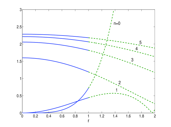
Figure 2: The curves show $(n^{3}+1)^{-1}|\det{\mathbf{Z}}(r)|$ for $n=0,1,\ldots,5$. The material is isotropic with $\{c_{11},c_{66},\rho\}=\{4,1,1\}$ and $\{\omega,k_{z}\}=\{1,0.2\}$. The Riccati equation (58) for ${\mathbf{Z}}(r)$ was integrated to obtain the curves for $0<r\leq 1$, starting from $r=0$ with the known ${\mathbf{Z}}_{0}$ of eq. (7.1.3). For $r>1$ the system equations (25) were integrated and eqs. (60) and (61) used to find ${\mathbf{Z}}(r)$, starting from the Riccati solution at $r=1$.

The initial step in the computation requires the value of the central impedance, which was calculated using eqs. (90) and (91) for $n=0$ and the formula ${\mathbf{Z}}_{0}=i{\mathbf{L}}_{1}{\mathbf{A}}_{1}^{-1}$ for $n>0$, see (54)₂, with ${\mathbf{A}}_{1}$, ${\mathbf{L}}_{1}$ defined by the numerical spectral decomposition of ${\mathbf{g}}_{0}(0)$ and the appropriate selection of its three eigenvalues with positive real part. It was confirmed that the computed ${\mathbf{Z}}_{0}$ satisfied the algebraic Riccati equation (59), with error always less than $10^{-12}$. Numerical integration of equations (58) and (60) was accomplished using the Runge-Kutta (4,5) routine in Matlab. In order to assess the accuracy of the numerical results the computed matrix ${\mathbf{Z}}_{comp}(r)$ and the analytical solution for ${\mathbf{Z}}(r)$ of (117) were compared. For the examples shown in Figure 2 it was found that the spectral norm of the difference satisfied $\|{\mathbf{Z}}_{comp}(r)-{\mathbf{Z}}(r)\|_{2}<10^{-4}$ at all points. The curves in Figure 2 use $r=1$ as the ‘cross-over’ coordinate, but similar accuracy was found for other values as long as they lie below the first singularity of ${\mathbf{Z}}(r)$, which for the parameters considered is $r_{*}>2$. In all cases the transition from the Riccati to the matricant based solution was found to be smooth.

This numerical procedure is designed to handle the coordinate-based singularity present in the system equations (22) at $r=0$, and can be continued, in principle, to any finite $r$. At the same time the computed impedance ${\mathbf{Z}}(r)$ will grow without bound at discrete values of $r>0$ associated with waveguide modes of the traction-free cylinder. The point of the algorithm is that it will continue to provide accurate solution regardless of the presence of two distinct types of singularity at $r=0$ and at finite values.

8 Conclusion

Impedance matrices appropriate to cylindrically anisotropic radially inhomogeneous elastic materials have been defined and procedures for their determination developed. In the process a new impedance matrix has been revealed as of central importance for wave motion in cylinders with on-axis material. The solid-cylinder impedance matrix is a characteristic property of the cylinder, with no free parameters apart from frequency and axial wavenumber. The impedance may be defined as the unique continuation of its on-axis limit, the central-impedance matrix, which is a simpler object dependent only on (a subset of) the elastic moduli. Two methods have been described for constructing the solid cylinder impedance at $r>0$, one based on a Frobenius series solution, the other using a differential Riccati equation. In addition to providing practical means for computation, as has been demonstrated for the latter approach, the methods shed light on the structural properties of the impedances. The Frobenius solution offers direct proof of uniqueness and Hermiticity, while the Riccati solution provides a stable method to integrate the otherwise singular system of equations at $r=0$. The radiation impedance matrix, suitable for infinite radial domains, has been defined and its properties delineated. We have found it instructive to compare the cylindrical impedance matrices with the surface wave impedance for a homogeneous half-space. The central-impedance matrix is the negative semi-definite counterpart of the static surface impedance, and the large $r$ limit of the radiation impedance is closely related to the surface wave impedance with $v=\omega/k_{z}$.

One purpose in developing these impedance matrices is the significant advantage offered by the impedance approach in solving boundary value problems. The solid-cylinder impedance matrix provides perhaps the simplest method to arrive at the dispersion equation of a radially inhomogeneous solid cylinder. In this regard we note that, by analogy with the conditional $(3\times 3)$ and two-point ($6\times 6$) impedances of an annulus [12], the eigenvalues of the solid-cylinder impedance should be monotonic in $\omega$ at any fixed $k_{z}$, which can be helpful for finding numerical solutions of the dispersion equation. In a wider context, the impedance matrix in conjunction with the radiation impedance, can serve in formulating scattering of acoustic and elastic waves from solid cylinders. Other applications that we envisage include the use of impedance matrices for solving problems with distributed forces within the cylinder, and applications involving 2D-inhomogeneous or laterally bounded planar and cylindrical waveguides [42, 43] where the algebraic impedance matrices discussed here become differential operators.

Another no less important reason for investigating the impedance matrix in the cylindrical context is that it affords new insights on the nature of elastodynamic solutions in anisotropic elasticity. It is remarkable, for instance, to find the Riccati equation appear as a natural method for solution in cylindrical elastodynamics. The Riccati equation, in fact, implies that the central-impedance solves an algebraic Riccati equation, which in turn leads to direct methods for its evaluation using analogies with the surface wave impedance. Differential Riccati equations have been found useful in few elastic wave settings, e.g. [3, 4, 5, 21, 42]. Its appearance here suggests it has wider potential application in computational elastodynamics.

Acknowledgment. ANN wishes to express his gratitude to the Laboratoire de Méchanique Physique (LMP) of the Université Bordeaux 1 for their hospitality.

References

- Lothe and Barnett [1976] J. Lothe and D. M. Barnett. On the existence of surface-wave solutions for anisotropic elastic half-spaces with free surface. J. Appl. Phys., 47(2):428–433, 1976.
- Barnett and Lothe [1985] D. M. Barnett and J. Lothe. Free surface (Rayleigh) waves in anisotropic elastic half-spaces: The surface impedance method. Proc. R. Soc. A, 402(1822):135–152, 1985. doi: 10.2307/2397800.
- Biryukov [1985] S. V. Biryukov. Impedance method in the theory of elastic surface waves. Sov. Phys. Acoust., 31:350–354, 1985.
- Biryukov et al. [1995] V. Biryukov, Yu. V. Gulyaev, V. V. Krylov, and V. P. Plessky. Surface Acoustic Waves in Inhomogeneous Media. Springer, Berlin, 1995.
- Caviglia and Morro [2002] G. Caviglia and A. Morro. Wave reflection and transmission from anisotropic layers through Riccati equations. Q. J. Mech. Appl. Math., 55:93–107, 2002.
- Honein et al. [1991] B. Honein, A. M. B. Braga, P. Barbone, and G. Herrmann. Wave propagation in piezoelectric layered media with some applications. J. Intell. Mater. Sys. Struct., 2(4):542–557, October 1991. doi: 10.1177/1045389X9100200408.
- Wang and Rokhlin [2002] L. Wang and S. I. Rokhlin. Recursive impedance matrix method for wave propagation in stratified media. Bull. Seism. Soc. Am., 92:1129–1135, 2002.
- Hosten and Castaings [2003] B. Hosten and M. Castaings. Surface impedance matrices to model the propagation in multilayered media. Ultrasonics, 41(7):501–507, September 2003. doi: 10.1016/S0041-624X(03)00167-7.
- Shuvalov [2000] A. L. Shuvalov. On the theory of wave propagation in anisotropic plates. Proc. R. Soc. A, 456(2001):2197–2222, 2000. doi: 10.1098/rspa.2000.0609.
- Shuvalov et al. [2004] A. Shuvalov, O. Poncelet, and M. Deschamps. General formalism for plane guided waves in transversely inhomogeneous anisotropic plates. Wave Motion, 40(4):413–426, October 2004. doi: 10.1016/j.wavemoti.2004.02.008.
- Shuvalov et al. [2008] A. Shuvalov, E. Le Clezio, and G. Feuillard. The state-vector formalism and the Peano-series solution for modelling guided waves in functionally graded anisotropic piezoelectric plates. Int. J. Engng. Sc., 46(9):929–947, September 2008. doi: 10.1016/j.ijengsci.2008.03.007.
- Shuvalov [2003a] A. L. Shuvalov. A sextic formalism for three-dimensional elastodynamics of cylindrically anisotropic radially inhomogeneous materials. Proc. R. Soc. A, 459(2035):1611–1639, 2003a. Note misprints: There is a on the r.h.s. of eq. (2.8); the left off-diagonal blocks mentioned below (2.16) are positive semi-definite; appearing below eqs. (4.1) and (4.4) must be replaced by .
- Mirsky [1966] I. Mirsky. Three-dimensional and shell-theory analysis for axisymmetric vibrations of orthotropic shells. J. Acoust. Soc. Am., 39(3):549–555, 1966.
- Ohnabe and Nowinski [1971] H. Ohnabe and J. L. Nowinski. On the propagation of flexural waves in anisotropic bars. Arch. Appl. Mech. (Ingenieur Archiv), 40(5):327–338, September 1971. doi: 10.1007/BF00533149.
- Chou and Achenbach [1972] F. H. Chou and J. D. Achenbach. Three-dimensional vibrations of orthotropic cylinders. J. Engng. Mech. ASCE, 98(4):813–823, 1972.
- Srinivas [1974] S. Srinivas. Analysis of laminated composite circular cylindrical shells with general boundary conditions. Technical report, NASA TR-R-412, 1974.
- Markus [1995] S. Markus. Wave motion in a three-layered, orthotropic-isotropic-orthotropic, composite shell. J. Sound. Vib., 181(1):149–167, March 1995. doi: 10.1006/jsvi.1995.0131.
- Martin and Berger [2001] P. A. Martin and J. R. Berger. Waves in wood: free vibrations of a wooden pole. J. Mech. Phys. Solids, 49(5):1155–1178, May 2001. doi: 10.1016/S0022-5096(00)00068-5.
- Soldatos [1994] K. P. Soldatos. Review of three dimensional dynamic analyses of circular cylinders and cylindrical shells. Appl. Mech. Rev., 47(10):501–516, 1994.
- Shuvalov [2003b] A. L. Shuvalov. The Frobenius power series solution for cylindrically anisotropic radially inhomogeneous elastic materials. Q. J. Mech. Appl. Math., 56(3):327–345, August 2003b. doi: 10.1093/qjmam/56.3.327. Note the misprints in eq. (5) (the lower off-diagonal block of ); on 1st line of p. 330 (should read ”If is semisimple…”), in the ordering below eq. (19); on 3rd line above eq. (35) (should read ”tetragonal with or higher…”); in eq. (39) (one of two successive entries should be ); in equation on p. 336 (the factor is missing); in eq. (43) (”” should be ””), and eq. (61) ( should be the same one line below); in eq. (52) (a common factor is missing), and in eq. (53) whose correct form is where , is real, and .
- Destrade et al. [2009] M. Destrade, A. Ní Annaidh, and C. Coman. Bending instabilities of soft biological tissues. Int. J. Solids Struct., 46(25-26):4322–4330, December 2009. doi: 10.1016/j.ijsolstr.2009.08.017.
- Pease [1965] M. C. Pease. Methods of Matrix Algebra. Academic Press, New York, 1965.
- Coddington and Carlson [1997] E. A. Coddington and R. Carlson. Linear Ordinary Differential Equations. SIAM, Philadelphia, 1997.
- Ting [1996a] T. C. T. Ting. Pressuring, shearing, torsion and extension of a circular tube or bar of cylindrically anisotropic material. Proc. R. Soc. A, 452(1954):2397–2421, November 1996a. doi: 10.1098/rspa.1996.0129.
- Lekhnitskii [1963] S. G. Lekhnitskii. Theory of Elasticity of an Anisotropic Elastic Body. Holden-Day, San Francisco, 1963.
- Shuvalov and Every [2002] A. V. Shuvalov and A. G. Every. Some properties of surface acoustic waves in anisotropic-coated solids, studied by the impedance method. Wave Motion, 36:257–253, 2002. doi: 10.1016/S0165-2125(02)00013-6.
- Ingebrigtsen and Tonning [1969] K. A. Ingebrigtsen and A. Tonning. Elastic surface waves in crystals. Phys. Rev., 184(3):942–951, Aug 1969. doi: 10.1103/PhysRev.184.942.
- Chadwick and Smith [1977] P. Chadwick and G. D. Smith. Foundations of the theory of surface waves in anisotropic elastic materials. Adv. Appl. Mech., 17:303–376, 1977.
- Ting [1996b] T. C. T. Ting. Anisotropic elasticity: Theory and Applications. Oxford University Press, 1996b.
- Barnett and Lothe [1973] D. M. Barnett and J. Lothe. Synthesis of the sextic and the integral formalism for dislocations, Greens functions, and surface waves in anisotropic elastic solids. Phys. Norv., 7:13–19, 1973.
- Barnett and Lothe [1974] D. M. Barnett and J. Lothe. Consideration of the existence of surface wave (Rayleigh wave) solutions in anisotropic elastic crystals. J. Phys. F: Met. Phys., 4(5):671–686, 1974. doi: 10.1088/0305-4608/4/5/009.
- Roberts [1980] J. D. Roberts. Linear model reduction and solution of the algebraic Riccati equation by use of the sign function. Internat. J. Control, 32(4):677–687, 1980.
- Kenney and Laub [1995] C. S. Kenney and A. J. Laub. The matrix sign function. IEEE Trans. Automat. Control, 40(8):1330–1348, 1995.
- Higham [2008] N. J. Higham. Functions of matrices: Theory and computation. 2008.
- Higham [1994] N. J. Higham. The matrix sign decomposition and its relation to the polar decomposition. Linear Algebra Appl., 212/213:3–20, 1994.
- Mielke and Fu [2004] A. Mielke and Y. B. Fu. Uniqueness of the surface-wave speed: A proof that is independent of the Stroh formalism. Math. Mech. Solids, 9(1):5–15, February 2004. doi: 10.1177/1081286503035196.
- Chadwick [1990] P. Chadwick. The behaviour of elastic surface waves polarized in a plane of material symmetry. I. General analysis. Proc. R. Soc. A, A430:213–240, 1990.
- Barnett et al. [1992] D. M. Barnett, P. Chadwick, and J. Lothe. The behaviour of elastic surface waves polarized in a plane of material symmetry. Addendum to part I. Proc. R. Soc. A, A433:699–710, 1992.
- Fu and Mielke [2002] Y. B. Fu and A. Mielke. A new identity for the surface-impedance matrix and its application to the determination of surface-wave speeds. Proc. R. Soc. A, 458(2026):2523–2543, 2002. doi: 10.2307/3067326.
- Buchwald [1959] V. T. Buchwald. Elastic waves in anisotropic media. Proc. R. Soc. A, 253:563–580, 1959.
- Rahman and Ahmad [1998] A. Rahman and F. Ahmad. Representation of the displacement in terms of scalar functions for use in transversely isotropic materials. J. Acoust. Soc. Am., 104(6):3675–3676, 1998.
- Pagneux and Maurel [2006] V. Pagneux and A. Maurel. Lamb wave propagation in elastic waveguides with variable thickness. Proc. R. Soc. A, 462(2068):1315–1339, April 2006. doi: 10.1098/rspa.2005.1612.
- Getman and Ustinov [1990] I. P. Getman and Yu. A. Ustinov. Wave propagation in an elastic longitudinally inhomogeneous cylinder. J. Appl. Math. Mech., 54:83–87, 1990.