Magnetic miniband and magnetotransport property of a graphene superlattice

Abstract

The eigen energy and the conductivity of a graphene sheet subject to a one-dimensional cosinusoidal potential and in the presence of a magnetic field are calculated. Such a graphene superlattice presents three distinct magnetic miniband structures as the magnetic field increases. They are, respectively, the triply degenerate Landau level spectrum, the nondegenerate minibands with finite dispersion and the same Landau level spectrum with the pristine graphene. The ratio of the magnetic length to the period of the potential function is the characteristic quantity to determine the electronic structure of the superlattice. Corresponding to these distinct electronic structures, the diagonal conductivity presents very strong anisotropy in the weak and moderate magnetic field cases. But the predominant magnetotransport orientation changes from the transverse to the longitudinal direction of the superlattice. More interestingly, in the weak magnetic field case, the superlattice exhibits half-integer quantum Hall effect, but with large jump between the Hall plateaux. Thus it is different from the one of the pristine graphene.

I introduction

Since or prior to the experimental acquirement of graphenenovoselov , an atomically thin graphitic sheet, its electronic properties and potential applications were widely investigated. It was experimentally demonstrated that graphene is a gapless semiconductor materialnovoselov ; novoselov2 . In the Brillouin zone of graphene, there are two inequivalent touching points between the valence and conduction bands, called the Dirac pointsZhang . In the low energy region relative to the Dirac points, the electron or hole follows a linear dispersion relationZhang ; zheng . Thus, two massless Dirac fermion systems form in the vicinity of two Dirac points. Such an electron structure is responsible for most interesting electronic properties unique to graphenenovoselov2 ; Zhang ; zheng ; Katsnelson . When a superlattice structure is established on a graphene sheet, the massless Dirac fermion is subject to a periodic modulation by the superlattice potential. Such a situation indicates that a graphene superlattice(GSL) perhaps exhibits unusual electronic characteristics, unlike both the pristine graphene and the ordinary semiconductor materialPark1 ; Park2 ; Brey ; Barbier ; Wang . Experimentally, many types of GSL have been fabricated and investigated. For example, electron-beam induced deposition of adsorbates on graphene membranes creates a dot array with a period of 5 nmMeyer ; Epitaxially growth of graphene on some metallic substrates can form periodic pattern of supercellPletikosi ; Diaye ; Vazquez ; Marchini . These experimental progresses certainly make the theoretical studies and device applications of GSLs realistic.

Accompanying the relevant experimental work, theoretical studies predicted many interesting electronic properties of GSLs. For example, some recent theoretical work focused on a simple GSL which is constructed by exerting a one-dimensional strip-like or cosinusoidal periodic potential on a graphene sheetPark1 ; Park2 ; Brey ; Park3 ; Barbier . It was found that such a one-dimensional GSL presents multiple Dirac points even in one valley of the pristine graphenePark1 ; Brey . The dependence of the number of the Dirac points on the strength and period of the superlattice potential was analyzed in detail. Furthermore, when a vertical magnetic field is applied, the low-lying Landau levels(LLs) become degeneratePark2 . Accordingly, it was mentioned that the degeneracy of the LL accounts for the large jump of the Hall conductivity plateaux of the GSLPark2 ; Park3 . Albeit these existent theoretical results, the electron structure of such a GSL in the presence of a magnetic field has not yet been comprehensively revealed. For example, magnetic mini-bands will be established in the GSL. But such a band structure and its dependence on the magnetic field strength are yet unknown. The magnetic transport properties, namely, the diagonal and Hall conductivity spectra of the GSL, have not been calculated, which may be different from those of the pristine graphene.

In the present work, by taking the LL states of the pristine graphene as the basis set, we calculate the energy spectrum of the GSL in the presence of a magnetic field. We find that the degenerate LL spectrum is only an electron structure of the GSL in the weak field limit, namely, in the case that the magnetic length is much longer than the period of the GSL. On the other hand, when the magnetic length is smaller than the period of the GSL, the flat LLs evolve into magnetic minibands with finite dispersion. Furthermore, if the magnetic length is much smaller than the period of the GSL, i.e. the strong field case, the superlattice will restore the LL spectrum of the pristine graphene. As for the magnetotransport properties, the diagonal conductivity shows notable anisotropy, especially in the weak magnetic field case. The Hall conductivity shows indeed the large jumps between the adjacent plateaux in the low energy region, reflecting the degeneracy of the low-lying LLs. However, such a quantum Hall effect is destroyed in a stronger magnetic field when the flat LL spectrum is replaced by the dispersive magnetic mini-bands.

The rest of the paper is organized as follows: In section II the theoretical method to solve the electronic eigen-equation of the GSL in the presence of a vertical magnetic field is briefly elucidated. Then starting from the Kubo formula the conductivities are formulated in terms of Green function(GF). In section III, the numerical results about the spectra of the eigen energy, the density of states(DOS), the diagonal and Hall conductivities for the GSL are shown and discussed. Finally, in section IV the main results are briefly summarized.

II Structure and Theory

When a magnetic field is applied perpendicular to the sheet of a pristine graphene, the low-energy electron structure in one valley, say the K valley, can be well described by an effective-mass Hamiltonian. It takes a form aszheng

$${\cal\hat{H}}_{0}=\frac{\gamma}{\hbar}\left[\begin{array}[]{cc}0&\hat{\pi}_{-}\\ \hat{\pi}_{+}&0\\ \end{array}\right],$$ (1)

where $\gamma$ is a band parameter, $\hat{\pi}_{\pm}=\hat{\pi}_{x}\pm i\hat{\pi}_{y}$ with $\hat{\pi}_{\alpha}$ ($\alpha=x,y$) being the gauged electron momentum. In Landau gauge, one has $\hat{\pi}_{x}=\hat{p}_{x}$ and $\hat{\pi}_{y}=\hat{p}_{y}+eBx/c$, with $B$ denoting the magnetic field strength and $\hat{p}_{\alpha}=-i\hbar\partial_{\alpha}$ being the momentum operator. Noting that K and K’ valleys give the same physical result, hereafter we only treat the electron behavior in K valley. The Dirac point is taken as the zero energy.

The eigen-equation ${\cal\hat{H}}_{0}|nk\rangle=\varepsilon_{n}|nk\rangle$ can be solved analytically, which gives the LL spectrum of the pristine graphenezheng . It is

$$\varepsilon_{n}=\textup{sgn}(n)\hbar\omega_{c}\sqrt{|n|},$$ (2)

and the corresponding wavefunction of the LL state is given by

$$|nk\rangle=\frac{C_{n}}{\sqrt{L_{0}}}e^{-iky}\left[\begin{array}[]{c}\textup{sgn}(n)(-i){\phi_{|n|-1}}\\ \phi_{|n|}\end{array}\right].$$ (3)

In the above two equations, $\hbar\omega_{c}={\sqrt{2}\gamma}/l$. It is defined as the electron cyclotron energy with $l=\sqrt{c\hbar/eB}$ being the magnetic length. $L_{0}$ stands for the linear size of the graphene sheet. And $k$ is electronic wave vector in the $y$ direction. In addition, the normalization constant is

$$C_{n}=\left\{\begin{array}[]{cccc}1&&(n=0),\\ 1/\sqrt{2}&&(n\neq 0).\end{array}\right.$$ (4)

The relevant functions are defined as

$$\textup{sgn}(n)=\left\{\begin{array}[]{cccc}1&&(n>0),\\ 0&&(n=0),\\ -1&&(n<0),\end{array}\right.$$ (5)

and

$$\phi_{|n|}=\frac{1}{\sqrt{2^{|n|}|n|!\sqrt{\pi}\hskip 2.0ptl}}\textup{exp}\left[-\frac{1}{2}\left(\frac{x-x_{0}}{l}\right)^{2}\right]H_{|n|}\left(\frac{x-x_{0}}{l}\right),$$ (6)

where $x_{0}=l^{2}k$, is the center of the electronic harmonic motion; And $H_{n}(\xi)$ is the Hermite polynomial.

When we consider the electronic and transport properties of a GSL, we need to define a one-dimensional periodic potential along $x$ direction, in addition to the Hamiltonian ${\cal\hat{H}}_{0}$. We choose the cosinusoidal potential function given by

$$\hat{V}(x)={V_{0}\over 2}\textup{cos}(2\pi x/L).$$ (7)

It can model the periodic gate voltages applied on the graphene sheet. Thus, the electronic Hamiltonian of such a GSL in the presence of a vertical magnetic field is given by ${\cal\hat{H}}={\cal\hat{H}}_{0}+\hat{V}(x)$. Due to the presence of the periodic potential, it is impossible to obtain an analytical solution to the eigen-equation ${\cal\hat{H}}|\lambda k\rangle=E_{\lambda}(k)|\lambda k\rangle$. However, we can obtain the numerical results about it by the exact diagonalization technique. In doing so, we choose the LL state of the pristine graphene described above by Eqs(2-6) as the basis set. Then, we can readily find that the Hamiltonian matrix element is diagonal with respect to the electron wave vector $k$

$$\langle n^{\prime}k^{\prime}|{\cal\hat{H}}|nk\rangle=\big{[}\varepsilon_{n}\delta_{nn^{\prime}}+\langle n^{\prime}k|\hat{V}(x)|nk\rangle\big{]}\delta_{kk^{\prime}}.$$ (8)

In the above equation, the matrix element of periodic potential can be worked out analytically. It is given byKubo

$$\langle n^{\prime}k|\hat{V}(x)|nk\rangle=\frac{V_{0}C_{n^{\prime}}C_{n}}{4}\left[\textup{sgn}(n^{\prime}n)\big{(}J^{+}_{|n^{\prime}|-1,|n|-1}+\right.$$ (9)

$$\left.J^{-}_{|n|-1,|n^{\prime}|-1}\big{)}+J^{+}_{|n^{\prime}|,|n|}+J^{-}_{|n|,|n^{\prime}|}\right],$$

where

$$J^{\pm}_{{\scriptscriptstyle NN^{\prime}}} = (\pm i\beta)^{N_{1}-N_{2}}\left[\frac{N_{2}!}{N_{1}!}\right]^{1\over 2}\times$$

$$\!\exp\!\!\Big{[}\pm i{2\pi x_{0}\over L}-{\beta^{2}\over 2}\Big{]}L^{{\scriptscriptstyle(N_{1}-N_{2})}}_{\scriptscriptstyle{N_{2}}}(\beta^{2}),$$

with $\beta=\sqrt{2}\pi l/L$, $N_{1}=\max(N,N^{\prime})$ and $N_{2}=\min(N,N^{\prime})$. $L_{n}^{(r)}(\xi)$ stands for the associated Laguerre polynomials. It is defined as

$$L_{n}^{(r)}(\xi)=\Big{(}{{e^{\xi}\xi^{-r}}\over{n!}}\Big{)}{{d^{n}}\over{d\xi^{n}}}(e^{-\xi}\xi^{n+r}).$$ (11)

The eigen wavefunction of the GSL can be formally written as

$$|\lambda k\rangle=\sum_{n=-{\scriptscriptstyle N}_{c}}^{{\scriptscriptstyle N}_{c}}d_{n}^{\lambda}|nk\rangle.$$ (12)

The expansion coefficients $d_{n}^{\lambda}$’s, along with the corresponding eigen energy $E_{\lambda}(k)$, can be obtained by solving the eigen-problem of the Hamiltonian matrix defined above. In the actual calculation, we need to choose an appropriate cutoff index $N_{c}$ which makes the matrix dimension finite. Of course, such a cutoff should guarantee the stationary results about the low-lying energy levels.

By defining the retarded GF $G_{\lambda}(\omega,x_{0})=[{\omega-E_{\lambda}(k)+i\eta}]^{-1}$ with $\eta$ being a positive infinitesimal, the DOS can be expressed as

$$\rho(\omega) = -\frac{1}{\pi L_{0}^{2}}\sum_{\lambda,k}\textup{Im}G_{\lambda}(\omega,x_{0})$$

$$= -\frac{1}{2\pi^{2}l^{2}L}\sum_{\lambda}\int_{0}^{L}dx_{0}\textup{Im}G_{\lambda}(\omega,x_{0}).$$

According to Kubo’s linear response theory, the diagonal and Hall conductivities of a two-dimensional electron system in the presence of a magnetic field can be formulated in terms of GF as

$$\sigma_{\alpha\alpha}(\varepsilon)=\frac{e^{2}\hbar}{\pi L_{0}^{2}}\textup{Tr}\big{[}\hat{v}_{\alpha}\textup{Im}\hat{G}(\varepsilon)\hat{v}_{\alpha}\textup{Im}\hat{G}(\varepsilon)\big{]},$$ (14)

and

$$\sigma_{xy}(\varepsilon)=\frac{ie^{2}\hbar}{\pi L_{0}^{2}}\int_{0}^{\varepsilon}d\omega\textup{Tr}\big{[}\hat{v}_{x}\textup{Im}\hat{G}(\omega)\hat{v}_{y}\frac{d}{d\omega}\textup{Re}\hat{G}(\omega)$$ (15)

$$-\hat{v}_{y}\textup{Im}\hat{G}(\omega)\hat{v}_{x}\frac{d}{d\omega}\textup{Re}\hat{G}(\omega)\big{]}.$$

In the above two formulae, the retarded GF operator is defined as $\hat{G}(\omega)=[\omega-\hat{\cal{H}}+i\eta]^{-1}$. $\varepsilon$ denotes the chemical potential. $\hat{v}_{\alpha}=(i/\hbar)[\hat{H},\hat{\alpha}]=(\gamma/\hbar)\hat{\sigma}_{\alpha}$ is the velocity operator which is associated with the Pauli matrix $\hat{\sigma}_{\alpha}$. When applying these formulae to the above GSL, by a straightforward derivation we can obtain the expressions of the conductivities, given by

$$\sigma_{\alpha\alpha}(\varepsilon) = (\frac{e^{2}}{h})\frac{\hbar^{2}}{\pi Ll^{2}}\int_{0}^{L}dx_{0}\sum_{\lambda,\lambda^{\prime}}$$

$$\text{Im}G_{\lambda}(\varepsilon,x_{0})\text{Im}G_{\lambda^{\prime}}(\varepsilon,x_{0})\left|\langle\lambda k|\hat{v}_{\alpha}|\lambda^{\prime}k\rangle\right|^{2},$$

and

$$\sigma_{xy}(\varepsilon) = (\frac{e^{2}}{h})\frac{2\hbar^{2}}{\pi Ll^{2}}\int_{0}^{\varepsilon}d\omega\int_{0}^{L}dx_{0}\sum_{\lambda,\lambda^{\prime}}\text{Im}G_{\lambda^{\prime}}(\omega,x_{0})$$

$$\text{Re}[G_{\lambda}(\omega,x_{0})]^{2}\text{Im}[\langle\lambda k|\hat{v}_{x}|\lambda^{\prime}k\rangle\langle\lambda k|\hat{v}_{y}|\lambda^{\prime}k\rangle].$$

The matrix elements of the velocity operators involved in the above two expressions are given by

$$\langle\lambda k|\hat{v}_{x}|\lambda^{\prime}k\rangle = -i{\gamma\over\hbar}\sum_{m,n}d_{m}^{\lambda^{\prime}}d_{n}^{\lambda}C_{m}C_{n}$$

$$\left[\text{sgn}(m)\delta_{|m|-1,|n|}-\text{sgn}(n)\delta_{|m|,|n|-1}\right],$$

and

$$\langle\lambda k|\hat{v}_{y}|\lambda^{\prime}k\rangle = {\gamma\over\hbar}\sum_{m,n}d_{m}^{\lambda^{\prime}}d_{n}^{\lambda}C_{m}C_{n}$$

$$\left[\text{sgn}(m)\delta_{|m|-1,|n|}+\text{sgn}(n)\delta_{|m|,|n|-1}\right].$$

We can readily prove that the two relations, $\langle\lambda k|\hat{v}_{x}|\lambda k\rangle=0$ and $\langle\lambda k|\hat{v}_{y}|\lambda k\rangle=(1/\hbar)\partial E(k)/\partial k$, always hold true for any state. These relations are useful for us to analyze the numerical results about the magnetotransport property.

III Numerical results

We are now in a position to perform the numerical calculations about the electronic and transport properties of the GSL in the presence of a magnetic field, according to the theoretical approach given above. First of all, we calculate the electronic eigen energy spectrum for the cases of different magnetic fields. We take the cutoff index $N_{c}=1200$ which ensures the reliable result about the low-lying eigen energies close to the Dirac point. These spectra of a GSL are shown in Fig.1. The relevant parameters of the GSL satisfy the relation $V_{0}=6\pi\varepsilon_{{}_{L}}$ with $\varepsilon_{{}_{L}}=\gamma/L$. According to previous workPark2 ; Park3 , such a GSL displays triple Dirac points in one valley of the pristine graphene in the case of zero magnetic field. We reproduce such a result by choosing the plane waves as the basis set to establish the Hamiltonian matrix of the GSL in the absence of a magnetic field. Such a dispersion relation is shown in Fig.1(a). In Fig.1(b) some low-lying eigen energies are shown as functions of the electron wavevector $k$(rescaled as $x_{0}$) for a relatively weak magnetic field. The corresponding magnetic length is larger than the period of the GSL. We can see that these eigen energies scarcely depend on $x_{0}$. This is a reasonable result, because that the matrix elements of the Hamiltonian hardly depend on the central position of the LL states when the magnetic length is much larger than the period of the GSL. Hence the eigen energies form the flat magnetic minibands. These flat minibands shown in Fig.1(b) can be viewed as the LL spectrum of the GSL. However, these levels are not exactly dispersionless, which can be clearly seen from the insets which blow up the weak dispersion. Besides, the level distribution in Fig.1(b) is different from the LL spectrum of the pristine graphene. We can see from this figure that the three energy levels at the Dirac point are nearly degenerate. So are the two groups of the levels near the Dirac points. These results verify the LL degeneracy in the GSL concluded in previous work by using a distinct theoretical approachPark2 ; Park3 . When the magnetic field increases, the flat LL spectrum changes into dispersive magnetic mini-bands. Such a situation is shown in Fig.1(c) where the magnetic length is smaller than the period of the GSL by one order of magnitude. Hereafter we call such a case, namely, the occurrence of the dispersive magnetic mini-bands, as the moderate field case. Fig.4(d) shows the eigen energy spectrum when the magnetic length is far smaller than the period of the GSL. We can see that such a strong magnetic field restores the eigen energy spectrum to the LL spectrum of the pristine graphene, described by Eq.(2). This is because that in such a strong field case the periodic potential of GSL can be viewed as a small perturbation which only gives a trivial correction to the LL spectrum of the pristine graphene.

Figure 1: Low-lying eigen energies versus electronic wavevector k (rescaled as $x_{0}$ when a magnetic field is present) of a GSL with $V_{0}=6\pi\varepsilon_{\scriptscriptstyle L}$ and $\varepsilon_{\scriptscriptstyle L}=\gamma/L$. (a) The dispersion relation in the zero magnetic field case. The electronic wavevector along $x$ direction is fixed at $k_{x}=0$. (b) The weak field case, i.e. $l=2.0L$. The insets show the weak dispersion of the nearly degenerate levels in detail.(c) The moderate field case with $l=0.1L$ and (d) the strong field case with $l=0.001L$.

In order to see the influence of the magnetic field on the eigen energy spectrum of the GSL more clearly, in Fig.2 we show the eigen energies as functions of the magnetic length for a specific wavevector at $x_{0}=0$. We can see that in the moderate field regime the eigen energies depend sensitively on the variation of the magnetic field. In addition, in the weak field limit all the LLs tend to triply degenerate, which follows the triple Dirac points of the GSL. In Fig.3 we show the calculated DOS for such a GSL. The weak field case is shown in Fig.3(a). The sharp peaks in such a DOS spectrum correspond to LLs as shown in Fig.1(b). Noting that the three high peaks near the Dirac point arise from the triple degeneracy of these LLs. In the moderate field case, as shown in Fig.3(b), the DOS spectrum exhibits a series of peaks. These peaks indicate the singularities in the DOS, which correspond to the minima and maxima of the magnetic mini-bands as shown in Fig.1(c). In the strong field case shown in Fig.3(c), the DOS spectrum is almost the same as that of the pristine graphene in the presence of a magnetic field.

Figure 2: Low-lying eigen energies versus the magnetic length of a GSL with $V_{0}=6\pi\varepsilon_{\scriptscriptstyle L}$ at $x_{0}=0$.

Figure 3: The DOS spectrum of the GSL for (a) the weak, (b) the moderate and (c) the strong magnetic field cases, respectively.

Now we turn to study the magnetotransport properties of the GSL. The diagonal conductivity is calculated as a function of the chemical potential. And the calculated results are shown in Fig.4. From Fig.4(a) we can see that in the weak field case $\sigma_{xx}$ is larger than $\sigma_{yy}$. It indicates that the diagonal conductivity shows a strong anisotropy. We have known that the average velocity $\langle\lambda k|\hat{v}_{x}|\lambda k\rangle=0$ for any eigen-state. Besides, in the weak field case the average velocity along $y$ direction is ignorably small, namely, $\langle\lambda k|\hat{v}_{y}|\lambda k\rangle=(1/\hbar)\partial E_{\lambda}(k)/\partial k\approx 0$, due to the flat band structure as shown in Fig.1(b). Therefore, the diagonal conductivity in the weak field case is determined by the interband contributions. From the numerical calculation we find that the matrix elements $\langle\lambda k|\hat{v}_{x}|\lambda^{\prime}k\rangle$ are notably larger than $\langle\lambda k|\hat{v}_{y}|\lambda^{\prime}k\rangle$ for any two distinct eigen-states. As a result, the conductivity in $x$ direction is larger than that in $y$ direction in the weak field case. In fact, the anisotropy of the diagonal conductivity arises from the anisotropic band structure around each Dirac points of the GSL. Previous work reported that the band structure of the GSL is notably anisotropic. Therefore, $\langle\hat{v}_{x}\rangle>\langle\hat{v}_{y}\rangle$ and $\sigma_{xx}>\sigma_{yy}$ holds true in zero magnetic field caseBarbier . We can infer that such an anisotropic band structure at each Dirac point of the GSL also controls the anisotropy in the electronic magnetotransport process presented here. The anisotropy in the diagonal conductivity remains in the moderate field case. However, opposite to the weak field case, the diagonal conductivity $\sigma_{xx}$ becomes the smaller one. In Fig.4(b) we can see that $\sigma_{yy}$ is nearly 10 times $\sigma_{xx}$. Moreover, the peaks of $\sigma_{xx}$ just correspond to the dips of $\sigma_{yy}$. We can explain these features in the following way. The magnetotransport properties of the GSL in the moderate field case are determined by the dispersive magnetic mini-bands. Then the average velocity along $y$ direction takes a nonzero value in any mini-band, except at the band-edges. Namely, $\langle\hat{v}_{y}\rangle=\langle\lambda k|\hat{v}_{y}|\lambda k\rangle=(1/\hbar)\partial E_{\lambda}(k)/\partial k\neq 0$. In contrast to it, the average value of the velocity along $x$ direction is always equal to zero, i.e. $\langle\lambda k|\hat{v}_{x}|\lambda k\rangle=0$ in any state. Such a result means that $\sigma_{yy}$ has an intraband contribution, but the $\sigma_{xx}$ does not. From Eq.(II), the formula about the diagonal conductivity, we can see that $\sigma_{yy}$ is mainly determined by the intraband term which is proportional to $|\langle\lambda k|\hat{v}_{y}|\lambda k\rangle|^{2}$. At the minimum and the maximum of a specific mini-band, one has $\langle\lambda k|\hat{v}_{y}|\lambda k\rangle=0$. This indicates that the dips in the $\sigma_{yy}$ spectrum occur at these positions. On the other hand, the conductivity $\sigma_{xx}$ lacks the intraband contribution. Furthermore, the interband terms depend on the DOS of the magnetic mini-bands involved. This means that the conductivity peaks in the $\sigma_{xx}$ spectrum occur at the singularities of the DOS. And these singularities just correspond to the minimum or the maximum of a mini-band. Fig.4(c) shows the diagonal conductivity spectra in the strong field case. We can see that the anisotropy disappears. And the conductivity spectrum is very similar to that of pristine graphene.

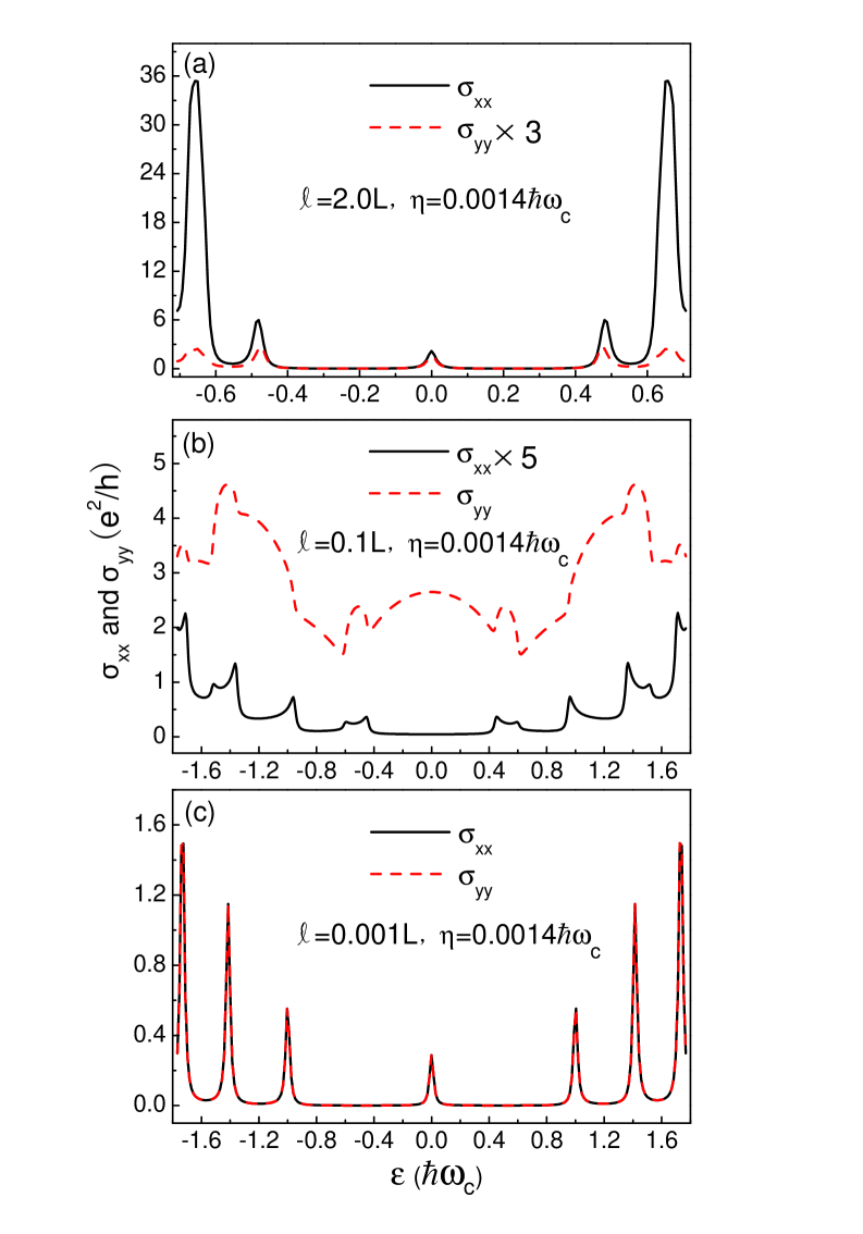
Figure 4: (Color online) The diagonal conductivities $\sigma_{xx}$ and $\sigma_{yy}$ versus the chemical potential for a GSL with $V_{0}=6\pi\varepsilon_{\scriptscriptstyle L}$ for some typical magnetic fields. (a) Magnetic length $l=2.0L$, (b) $l=0.1L$, and (c) $l=0.001L$. Noting that $\sigma_{yy}$ in (a) is multiplied by 3 and $\sigma_{xx}$ in (b) is multiplied by 5, in order to show these curves clearly.

The spectra of the Hall conductivity are shown in Fig.5 for the typical magnetic fields. At first, from Fig.5(a) we can see that in the weak field case the GSL exhibits the quantum Hall effect. But the resolvable Hall plateaux only appear at the positions: $\pm 3/2(e^{2}/h),\pm 9/2(e^{2}/h)$ near the Dirac point. This situation is different from the half-integer quantum Hall effect of the pristine graphene. In fact, such a quantum Hall effect just follows the degenerate LL spectrum (strictly speaking, the nearly degenerate LLs) in the weak field case as shown in Fig.1(b). The triply degenerate low-lying LLs and the conduction-valence band symmetry of the energy spectrum can well account for these plateaux shown in Fig.5(a). When the chemical potential goes away from the Dirac point, the dense LLs bring about the oscillating character in the Hall conductivity spectrum, instead of the plateau structure in the low energy region. In the moderate field case the flat LL spectrum disappears. As a result, Hall conductivity does not exhibit the well-defined quantum Hall plateaux. Such a result is shown in Fig.5(b). However, when the magnetic field increases to the strong field regime, the GSL exhibits the half-integer quantum Hall effect of the pristine graphene which is shown in Fig.5(c).

Figure 5: The Hall conductivity $\sigma_{xy}$ versus the chemical potential for a GSL with $V_{0}=6\pi\varepsilon_{\scriptscriptstyle L}$ for some typical magnetic fields. (a) Magnetic length $l=2.0L$, (b) $l=0.1L$, and (c) $l=0.001L$.

IV summary

We have studied the magnetic mini-band structure and the magnetotransport properties of a GSL formed by applying a one-dimensional cosinusoidal potential on a graphene sheet. At first, by using the LL states of the pristine graphene as the basis set and by solving the Hamiltonian matrix of the GSL, we have obtained the eigen energy spectrum of the GSL subject to a magnetic field. We found that the GSL exhibits three different electronic structures as the magnetic field increases. When the magnetic length is larger than the period of the GSL, namely, the weak field case, the GSL presents flat magnetic mini-bands near the Dirac point. These flat mini-bands can be viewed as the LL spectrum of the GSL. Unlike the LL spectrum of the pristine graphene, these LLs of GSL are nearly degenerate with three LLs as a group. And in the weak field limit the LL spectrum tends to triply degenerate. When the magnetic length is smaller than the period of the GSL by one order of magnitude, namely, the moderate field case, the flat LL spectrum in the weak field case is replaced by the dispersive mini-band structure. And when the magnetic field increases further to enter the strong field regime, namely, the magnetic length is far shorter than period of the GSL, the eigen energy spectrum gets back to the LL spectrum of the pristine graphene. Corresponding to these different electronic structures, the diagonal and Hall conductivities present different characteristics in different magnetic field regions. In the weak and moderate field cases, the diagonal conductivity exhibits a strong anisotropy. However, the predominant magnetotransport orientation changes from the transverse to the longitudinal direction of the superlattice when the magnetic field increases from the weak to the moderate case. More interestingly, in the weak field case the GSL presents large jumps between the Hall plateaux, different from the quantum Hall effect of the pristine graphene. This feature arises from the degenerate LL spectrum of the GSL in the weak field case.

V Acknowledgements

This work was financially supported by the National Nature Science Foundation of China under Grant No. NNSFC10774055, the Specialized Research Fund for the Doctoral Program of Higher Education (Grant No. SRFDP20070183130), and National Found for Fostering Talents of Basic Science (Grant No. J0730311).

References

- (1) K. S. Novoselov, A. K. Geim, S. V. Morozov, D. Jiang, Y. Zhang, S. V. Dubonos, I. V. Grigorieva, and A. A. Firsov, Science 306, 666 (2004).
- (2) K. S. Novoselov, A. K. Geim, S. V. Morozov, D. Jiang, M. I. Katsnelson, I. V. Grigorieva, S. V. Dubonos, and A. A. Firsov, Nature (London) 438, 197 (2005).
- (3) Y. B. Zhang, Y.-W. Tan, H. L. Stormer, and Ph. Kim, Nature (London) 438, 201 (2005).
- (4) Y. Zheng and T. Ando, Phys. Rev. B 65, 245420 (2002).
- (5) M. I. Katsnelson, K. S. Novoselov and A. K. Geim, Nature Phys. 2, 620-625 (2006).
- (6) C.-H. Park, L. Yang, Y.-W. Son, M. L. Cohen, and S. G. Louie, Phys. Rev. Lett. 101, 126804 (2008).
- (7) C.-H. Park, Y.-W. Son, L. Yang, M. L. Cohen, and S. G. Louie, Phys. Rev. Lett. 103, 046808 (2009).
- (8) L. Brey and H. A. Fertig, Phys. Rev. Lett. 103, 046809 (2009).
- (9) M. Barbier, P. Vasilopoulos, and F. M. Peeters, arXiv:1002.1442v1 (2010).
- (10) L.-G. Wang and S.-Y. Zhu, arXiv:1003.0732v1 (2010).
- (11) J. C. Meyer, C. O. Girit, M. F. Crommie, and A. Zettl, Appl. Phys. Lett. 92, 123110 (2008).
- (12) I. Pletikosić, M. Kralj, P. Pervan, R. Brako, J. Coraux, A. T. N’Diaye, C. Busse, and T. Michely, Phys. Rev. Lett. 102, 056808 (2009).
- (13) A. T. N’Diaye, J. Coraux, T. N Plasa, C. Busse, and T. Michely, New J. Phys. 10, 043033 (2008).
- (14) A. L. Vázquez de Parga, F. Calleja, B. Borca, M. C. G. Passeggi, Jr., J. J. Hinarejos, F. Guinea, and R. Miranda, Phys. Rev. Lett. 100, 056807 (2008).
- (15) S. Marchini, S. Günther, and J. Wintterlin, Phys. Rev. B 76, 075429 (2007).
- (16) See EPAPS Document No. E-PRLTAO-103-023932. For more information on EPAPS, see http://www.aip.org/ pubservs/epaps.html.
- (17) R. Kubo, S. J. Miyake and N. Hashitsume, in Solid State Physics, edited by F. Seitz and D. Turnbull, Vol. 17 (Academic Press, New York) 1965, p. 269.