Double detected spin-dependent quantum dot

Abstract

We study the dynamics of a spin-dependent quantum dot system, where an unsharp and a sharp detection scenario is introduced. The back-action of the unsharp detection related to the magnetization, proposed in terms of the continuous quantum measurement theory, is observed via the von Neumann measurement (sharp detection) of the electric charge current. The behavior of the average electron charge current is studied as a function of the unsharp detection strength $\gamma$, and features of measurement back-action are discussed. The achieved equations reproduce the quantum Zeno effect. Considering magnetic leads, we demonstrate that the measurement process may freeze the system in its initial state. We show that the continuous observation may enhance the transition between spin states, in contradiction with rapidly repeated projective observations, when it slows down. Experimental issue, such as the accuracy of the electric current measurement, is analyzed.

1 Introduction

The act of a quantum measurement is always performed by an external apparatus and involves complicated interactions with it. We are going to discuss the the back-action induced by the observer in the framework of unsharp measurements. The unsharp measurement extracts only partial information from an observable, so we introduce another detector with sharp detection. We are interested in the output of the sharp detection, which means that the unsharp measurement will be treated in a nonselective picture. The nonselective description represents a measurement, where our record of data was lost and replaced by an average over the data ensemble. The sharp detector also has its back-action, projecting the system randomly into its eigenstate, but now the readout will be kept and the further evolution of the system will be neglected. The double detected setup gives a possibility to analyze the so-called quantum Zeno effect (QZE) [1]. Rapidly repeated measurements give rise to the QZE, the suppression of transition between quantum states. In reality there are more complicated physical processes that take place during a quantum measurement, which can also cause QZE. The effect can be best understood in terms of the dynamic time evolution of the measured quantum systems.
 The double detection scenario is similar to the “indirect measurement” process [2], where the back action of a detector on the quantum system is observed by a third party, namely in our case by a sharp detector. In this context, the idea of detecting the measurement back-action related to one type of degree of freedom, with a detection scenario of an another type of degree of freedom, would be suitable for a future experiment. The charge detector is a convenient sharp detector type and its applicability in the semiconductor physics is very high. We choose the other detector to be a spin related, magnetization, detector. The application we have in mind is the spin-dependent single quantum dot, available in high quality due to massive progress in experimental technology. Spin manipulation and magnetization detection in quantum dot was studied in experiment by Ref. [3]. An external field, used for spin manipulation, can be viewed as an environment of the subsystem, the quantum dot. The whole of quantum system dynamics is reversible. Tracing out the environment’s degrees of freedom, we arrive at a non-unitary time evolution [4]. In general, all these non-unitary processes are connected through the Kraus-form (A), related to the completely positive mappings of the density matrices [5]. The subsystem’s non-unitary dynamic, imposed by the external field, can be interpreted as an unsharp measurement [6]. These manipulations are time-continuous, so we will study the magnetization detection in the frame of the continuous quantum measurement theory [7], avoiding the modeling of the detector system as a quantum system.
 While the system described above is similar to the spin-to-charge conversion in quantum dots [8, 9], the model of the unsharp detector is different. Here, the back-action of continuous quantum measurement on magnetization is investigated by a detected electric current, focusing on measurement back-action and on QZE in the spin states. The unsharp detector of the spin-to-charge conversion is modeled as a quantum point contact with a fixed coupling Hamiltonian. The theory presented here is broader, because the coupling between the unsharp detector and the system is choice of will, however has to be subject to a real experimental setup.
 For a possible experimental setup, the idea of the double detection in a spin-dependent quantum dot is reasonable, because quantum dots and also spin manipulations are important for the realization of qubits. The effects of spin decoherence related to quantum computing was studied by Refs. [10, 11, 12]. On the other hand the field of indirect measurements on quantum dots by means of Coulomb-coupled, quantum point contacts, single-electron transistors, or double quantum dot’s [9, 13]-[16] and the effects of QZE [13, 17] was studied by several works, and the concept of time-continuous measurement has been part of this field [9, 13, 14, 15, 18]. Previous research has monitored the sharp or unsharp detection of the observables related to the electron charge. While the work presented here examines the sharp detection of the electric current, it also contains an unsharp detection of a spin observable, the magnetization. The model proposed here is similar to the work of Ref. [18], where the authors studied the effect of the unsharp detection of electric current in a selective measurement scenario. For the difference from that work, we applied the model for the magnetization detection and we studied the evolution of the density matrix as a function of the electron number tunneled through the system.
 This article is organized as follows. In Sec. 2 we introduce our model. We derive the many-body Scrödinger equation including the terms of the continuous quantum measurement. We represent the density matrix as a function of the electron number in the right lead. The results of measurement back-action are shown and discussed in Secs. 3, 5. We investigate the accuracy of the electric charge current measurement in Sec. 4. General and continuous quantum measurement theories have a wide literature and to ensure the background of this work we present a short summary of this topic in the A and B using Refs. [7, 19, 20].

2 The model

We consider the spin-dependent quantum dot, subject of experimental work [21, 22], which is coupled to two separate electron reservoirs. The density of states in the reservoirs is very high (continuum), and the dot contains only isolated levels. We consider the highest energy level to be the state of two electrons with different spins ($s=\pm 1/2$) and therefore we include the effects of Coulomb interaction. The split of the one-electron energy level is done by a $z$-directed magnetic field $B_{z}$. We include a $x$-directed magnetic field $B_{x}$, describing the coherent oscillations between the spin up and spin down levels. The full Hamiltonian of the system reads

$$\hat{H}=\hat{H}_{D}+\hat{H}_{R}+\hat{H}_{I},$$ (1)

where

$$\hat{H}_{D} = \sum_{s}E_{s}\hat{a}^{\dagger}_{D,s}\hat{a}_{D,s}+U\hat{a}^{\dagger}_{D,\frac{1}{2}}\hat{a}_{D,\frac{1}{2}}\hat{a}^{\dagger}_{D,-\frac{1}{2}}\hat{a}_{D,-\frac{1}{2}}$$ (2)

$$+ \hbar\Omega(\hat{a}^{\dagger}_{D,\frac{1}{2}}\hat{a}_{D,-\frac{1}{2}}+\hat{a}^{\dagger}_{D,-\frac{1}{2}}\hat{a}_{D,\frac{1}{2}})$$

is the Hamiltonian of the quantum dot,

$$\hat{H}_{R}=\sum_{l,s}E_{l,s}\hat{a}^{\dagger}_{l,s}\hat{a}_{l,s}+\sum_{r,s}E_{r,s}\hat{a}^{\dagger}_{r,s}\hat{a}_{r,s}$$ (3)

is the Hamiltonian of the reservoirs (leads), and

$$\hat{H}_{I} = \sum_{l,s}\hbar(\omega_{l,s}\hat{a}^{\dagger}_{l,s}\hat{a}_{D,s}+\omega^{*}_{l,s}\hat{a}^{\dagger}_{D,s}\hat{a}_{l,s})$$ (4)

$$+ \sum_{r,s}\hbar(\omega_{r,s}\hat{a}^{\dagger}_{r,s}\hat{a}_{D,s}+\omega^{*}_{r,s}\hat{a}^{\dagger}_{D,s}\hat{a}_{r,s})$$

is the coupling Hamiltonian between the reservoirs and dot. The subscripts $l$ and $r$ enumerate correspondingly the (very dense) levels in the left and right leads. $\hat{a}_{D,s}$($\hat{a}^{\dagger}_{D,s}$) is the annihilation (creation) operator of spin $s$ in the quantum dot. $\hat{a}_{l/r,s}$($\hat{a}^{\dagger}_{l/r,s}$) is the annihilation (creation) operator of spin $s$ in the reservoir $l$ or $r$. $U$ is the Coulomb repulsion energy, the energy difference $E_{\frac{1}{2}}-E_{-\frac{1}{2}}$ is proportional to $B_{z}$ and the frequency $\Omega\sim B_{x}$. $E_{l,s}$ and $E_{r,s}$ are the one-electron energies with spin $s$ in the left and right leads. $\hbar\omega_{l,s}$ and $\hbar\omega_{r,s}$ are the respective tunneling amplitudes of spin $s$ between the left or right reservoir and the dot. (Fig. 1)
For simplicity, we restrict ourselves to a low temperature case, $T\to 0$. All the levels in the right and left lead are initially filled with electrons up to the Fermi energy $\mu_{r}$ and $\mu_{l}$, respectively. This situation will be treated as the “vacuum” state $|{0}\rangle$. We consider a large bias and that the energy levels are inside the band, $\mu_{l}\gg E_{s},U\gg\mu_{r}$. In the context of these conditions, the electric current flows only from left to right. The evolution of the whole system is described by the many-particle wave function. Taking into account the assumptions, the wave function is represented as

$$|{\Psi(t)}\rangle = \left[b_{0}(t)+\sum_{l}b_{l,\frac{1}{2}}(t)a_{D,\frac{1}{2}}^{\dagger}a_{l,\frac{1}{2}}+\sum_{l,s;r,s}b_{lr,s}(t)a_{r,s}^{\dagger}a_{l,s}+\sum_{l}b_{l,-\frac{1}{2}}(t)a_{D,-\frac{1}{2}}^{\dagger}a_{l,-\frac{1}{2}}\right.$$

$$+ \left.\sum_{l,-s<l^{\prime},s}b_{ll^{\prime},s}(t)a_{D,\frac{1}{2}}^{\dagger}a_{D,-\frac{1}{2}}^{\dagger}a_{l,-s}a_{l^{\prime},s}+\sum_{l,-s<l^{\prime},s;r}b_{ll^{\prime}r,\frac{1}{2}}(t)a_{D,\frac{1}{2}}^{\dagger}a_{r,-\frac{1}{2}}^{\dagger}a_{l,-s}a_{l^{\prime},s}\right.$$

$$+ \left.\sum_{l,s<l^{\prime},s^{\prime};r,s>r^{\prime},s^{\prime}}b_{ll^{\prime}rr^{\prime},ss^{\prime}}(t)\hat{a}^{\dagger}_{r,s}\hat{a}^{\dagger}_{r^{\prime},s^{\prime}}\hat{a}_{l,s}\hat{a}_{l^{\prime},s^{\prime}}+\sum_{l,-s<l^{\prime},s;r}b_{ll^{\prime}r,-\frac{1}{2}}(t)a_{D,-\frac{1}{2}}^{\dagger}a_{r,\frac{1}{2}}^{\dagger}a_{l,-s}a_{l^{\prime},s}+\ldots\right]|0\rangle,$$

where, for example $\sum_{l,-s<l^{\prime},s}$ is the sum over all states with energy $E_{l,-s}$ and $E_{l^{\prime},s}$ and with the condition $E_{l^{\prime},s}>E_{l,-s}$. The amplitudes represent the physical situations as: $|b_{0}(t)|^{2}$ the probability that the system is in the “vacuum” state at time $t$, $|b_{l,\frac{1}{2}}(t)|^{2}$ the probability that one electron with spin up was annihilated in the left reservoir and one electron with spin up created in the quantum dot at time $t$, and so on. The “vacuum” state $|{0}\rangle$ in this representation has the following properties:

$$\hat{a}^{\dagger}_{l,s}|{0}\rangle = 0,\,\,\hat{a}_{r,s}|{0}\rangle=0,\,\,\hat{a}^{\dagger}_{l,s}\hat{a}_{l,s}|{0}\rangle=|{0}\rangle,$$

$$\hat{a}_{r,s}\hat{a}^{\dagger}_{r,s}|{0}\rangle = |{0}\rangle,\,\,\hat{a}_{D,s}\hat{a}^{\dagger}_{D,s}|{0}\rangle=|{0}\rangle,\,\,.\,.\,.\,.\,.$$ (6)

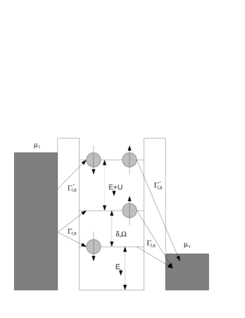
Figure 1: Schematic of the spin-dependent quantum dot model, including the left-to-right tunneling assumption and the energy differences between the considered levels.

Now, we apply the theory of continuous quantum measurement (B). The time evolution of the system in the presence of a time-continuous measurement of the magnetization, $\hat{M}=\hat{a}^{\dagger}_{D,\frac{1}{2}}\hat{a}_{D,\frac{1}{2}}-\hat{a}^{\dagger}_{D,-\frac{1}{2}}\hat{a}_{D,-\frac{1}{2}}$, is given by a modified Schrödinger equation:

$$d|\Psi\rangle=\Big{[} -\frac{i}{\hbar}\hat{H}dt-\frac{\gamma}{8}\left(\langle\hat{M}\rangle-\hat{M}\right)^{2}dt$$ (7)

$$-\frac{\sqrt{\gamma}}{2}\left(\langle\hat{M}\rangle-\hat{M}\right)dW\Big{]}|\Psi\rangle,$$

where $\langle\hat{M}\rangle=\langle\Psi|\hat{M}|\Psi\rangle$ is average detected magnetization and $W$ is the Wiener process. In order to derive this equation, we assumed that the detector bandwidth is bigger than the eigenfrequencies of the system, defined by the Hamiltonian $\hat{H}$. The main parameter of the theory, the detection performance (or detection strength), is defined as

$$\gamma=\frac{1}{\Delta t(\Delta M)^{2}},$$ (8)

where $\Delta t$ is the time-resolution (or, equivalently, the inverse bandwidth) of the detector (detecting the magnetization $\hat{M}$) and $\Delta M$ is the statistical error characterizing unsharp detection of the average value of the magnetization $\hat{M}$ in the period $\Delta t$.
Substituting eq. (2) into the equation of motion (7) using the Hamiltonian (1), we find a system of coupled differential equations for the amplitudes

$$db_{0}(t) = -i\sum_{l}\omega_{l,\frac{1}{2}}{b}_{l,\frac{1}{2}}(t)dt-i\sum_{l}\omega_{l,-\frac{1}{2}}{b}_{l,-\frac{1}{2}}(t)dt-\frac{\gamma}{8}\langle\hat{M}\rangle^{2}b_{0}(t)dt-\frac{\sqrt{\gamma}}{2}\langle\hat{M}\rangle b_{0}(t)dW,$$ (9)

$$db_{l,\frac{1}{2}}(t) = -i\frac{E_{\frac{1}{2}}-E_{l}}{\hbar}{b}_{l,\frac{1}{2}}(t)dt-i\omega^{*}_{l,\frac{1}{2}}{b}_{0}(t)dt-i\Omega{b}_{l,-\frac{1}{2}}(t)dt-i\sum_{l^{\prime}}\omega_{l^{\prime},-\frac{1}{2}}{b}_{ll^{\prime},-\frac{1}{2}}(t)dt$$ (10)

$$- i\sum_{r}\omega^{*}_{r,\frac{1}{2}}b_{lr,\frac{1}{2}}(t)dt-\frac{\gamma}{8}\left(\langle\hat{M}\rangle-1\right)^{2}b_{l,\frac{1}{2}}(t)dt-\frac{\sqrt{\gamma}}{2}\left(\langle\hat{M}\rangle-1\right)b_{l,\frac{1}{2}}(t)dW,$$

$$db_{lr,s}(t) = -i\frac{E_{r,s}-E_{l,s}}{\hbar}{b}_{lr,s}(t)dt-i\omega_{r,s}{b}_{l,s}(t)dt-i\omega_{r,-s}{b}_{l,-s}(t)dt-i\sum_{l^{\prime}}\omega_{l^{\prime},s}{b}_{ll^{\prime}r,s}(t)dt$$ (11)

$$- i\sum_{l^{\prime}}\omega_{l^{\prime},-s}{b}_{ll^{\prime}r,-s}(t)dt-\frac{\gamma}{8}\langle\hat{M}\rangle^{2}b_{lr,s}(t)dt-\frac{\sqrt{\gamma}}{2}\langle\hat{M}\rangle b_{lr,s}(t)dW,$$

$$db_{l,-\frac{1}{2}}(t) = -i\frac{E_{-\frac{1}{2}}-E_{l}}{\hbar}{b}_{l,-\frac{1}{2}}(t)dt-i\omega^{*}_{l,-\frac{1}{2}}{b}_{0}(t)dt-i\Omega{b}_{l,\frac{1}{2}}(t)dt-i\sum_{l^{\prime}}\omega_{l^{\prime},\frac{1}{2}}{b}_{ll^{\prime},\frac{1}{2}}(t)dt$$ (12)

$$- i\sum_{r,-\frac{1}{2}}\omega^{*}_{r}b_{lr,-\frac{1}{2}}(t)dt-\frac{\gamma}{8}\left(\langle\hat{M}\rangle+1\right)^{2}b_{l,-\frac{1}{2}}(t)dt-\frac{\sqrt{\gamma}}{2}\left(\langle\hat{M}\rangle+1\right)b_{l,-\frac{1}{2}}(t)dW,$$

$$db_{ll^{\prime},s}(t) = -i\frac{E_{s}+E_{-s}+U-E_{l}-E_{l^{\prime}}}{\hbar}{b}_{ll^{\prime},s}(t)dt-i\omega^{*}_{l^{\prime},s}{b}_{l,s}(t)dt-i\omega^{*}_{l,s}{b}_{l^{\prime},s}(t)dt$$ (13)

$$- i\omega^{*}_{l^{\prime},-s}{b}_{l,-s}(t)dt-i\omega^{*}_{l,-s}{b}_{l^{\prime},-s}(t)dt-i\sum_{r}\omega^{*}_{r,s}{b}_{ll^{\prime}r,s}(t)dt-i\sum_{r}\omega^{*}_{r,-s}{b}_{ll^{\prime}r,-s}(t)dt$$

$$- \frac{\gamma}{8}\langle\hat{M}\rangle^{2}b_{ll^{\prime},s}(t)dt-\frac{\sqrt{\gamma}}{2}\langle\hat{M}\rangle b_{ll^{\prime},s}(t)dW,$$

$$\cdots\cdots\cdots \cdots \cdots\cdots\cdots\,\,\,\cdots\,\,\,\cdots\cdots$$

The sharp measurement is represented by a electric current measurement, which is related to the accumulated charge in the right lead. In order to analyze this quantity we introduce the density matrix as a function of $n$, the number of electrons in the right lead. The Fock space of the quantum dot consists of only four possible states, namely: $|a\,\rangle=|0\rangle$ the dot is empty, $|b\,\rangle=|\uparrow\rangle$ the dot contains a spin up electron ($s=\frac{1}{2}$), $|c\,\rangle=|\downarrow\rangle$ the dot contains a spin down electron($s=-\frac{1}{2}$) and $|d\,\rangle=|\uparrow\downarrow\rangle$ is the fully occupied dot. In our notation, these probabilities are represented as follows:

$$\sigma_{aa}=\sum_{n}\sigma_{aa}^{(n)}=|b_{0}(t)|^{2}+\sum_{l,s;r,s}|b_{lr,s}(t)|^{2}+\ldots$$ (14)

$$\sigma_{bb} = \sum_{n}\sigma_{bb}^{(n)}=\sum_{l}|b_{l,\frac{1}{2}}(t)|^{2}+\sum_{l,-s<l^{\prime},s;r}|b_{ll^{\prime}r,\frac{1}{2}}(t)|^{2}$$ (15)

$$+ \ldots$$

$$\sigma_{bc} = \sum_{n}\sigma_{bc}^{(n)}=\sum_{l}b_{l,\frac{1}{2}}(t)b_{l,-\frac{1}{2}}^{*}(t)$$ (16)

$$+ \sum_{l,-s<l^{\prime},s;r}b_{ll^{\prime}r,\frac{1}{2}}(t)b_{ll^{\prime}r,-\frac{1}{2}}^{*}(t)+\ldots$$

$$\sigma_{cc} = \sum_{n}\sigma_{cc}^{(n)}=\sum_{l}|b_{l,-\frac{1}{2}}(t)|^{2}+\sum_{l,-s<l^{\prime},s;r}|b_{ll^{\prime}r,-\frac{1}{2}}(t)|^{2}$$ (17)

$$+ \ldots$$

$$\sigma_{dd}=\sum_{n}\sigma_{dd}^{(n)}=\sum_{l,-s<l^{\prime},s}|b_{ll^{\prime},s}(t)|^{2}+\ldots$$ (18)

We are going to investigate a nonselective continuous quantum measurement case, which means that we are only interested in the average over the different realization of the wave function $|{\Psi}\rangle$. As a first step, we apply the quantum Ito rules [23] for the product rule of differentiation,

$$d\big{(}|{\Psi}\rangle\langle{\Psi}|\big{)}=d|{\Psi}\rangle\langle{\Psi}|+|{\Psi}\rangle d\langle{\Psi}|+d|{\Psi}\rangle d\langle{\Psi}|.$$ (19)

Through this step the stochastic time evolution of the density matrix is defined. Now, we average over the realizations [24], where we use that $W$ is the standard Wiener process, a Gaussian random variable with zero mean value ($\mathbf{M}$) and variance $t$,

$$\mathbf{M}(dW)=0,\,\,d^{2}W=dt,\,\,d^{n}W=0,\,n>2.$$ (20)

In the context of the nonselective measurement we define the following matrix elements:

$$\rho_{aa}^{(n)} = \mathbf{M}(\sigma_{aa}^{(n)}),\,\rho_{bb}^{(n)}=\mathbf{M}(\sigma_{bb}^{(n)}),\,\rho_{bc}^{(n)}=\mathbf{M}(\sigma_{bc}^{(n)}),$$

$$\rho_{cc}^{(n)} = \mathbf{M}(\sigma_{cc}^{(n)}),\,\rho_{dd}^{(n)}=\mathbf{M}(\sigma_{dd}^{(n)}).$$ (21)

As a second step, we use the large bias assumption [25] and a straightforward calculation yields a chain differential equations for the density matrix elements defined in eq. (2)

$$\dot{\rho}_{aa}^{(n)} = -(\Gamma_{l,\frac{1}{2}}+\Gamma_{l,-\frac{1}{2}})\rho_{aa}^{(n)}+\Gamma_{r,\frac{1}{2}}\rho_{bb}^{(n-1)}+\Gamma_{r,-\frac{1}{2}}\rho_{cc}^{(n-1)}+\sqrt{\Gamma_{r,\frac{1}{2}}\Gamma_{r,-\frac{1}{2}}}(\rho_{bc}^{(n-1)}+\rho_{cb}^{(n-1)}),$$ (22)

$$\dot{\rho}_{bb}^{(n)} = i\Omega(\rho_{bc}^{(n)}-\rho_{cb}^{(n)})-(\Gamma^{\prime}_{l,-\frac{1}{2}}+\Gamma_{r,\frac{1}{2}})\rho_{bb}^{(n)}+\Gamma_{l,\frac{1}{2}}\rho_{aa}^{(n)}+\Gamma^{\prime}_{r,-\frac{1}{2}}\rho_{dd}^{(n-1)}$$ (23)

$$- \frac{\sqrt{\Gamma_{r,\frac{1}{2}}\Gamma_{r,-\frac{1}{2}}}+\sqrt{\Gamma^{\prime}_{l,\frac{1}{2}}\Gamma^{\prime}_{l,-\frac{1}{2}}}}{2}(\rho_{bc}^{(n)}+\rho_{cb}^{(n)}),$$

$$\dot{\rho}_{bc}^{(n)} = -i\delta\rho_{bc}^{(n)}+i\Omega(\rho_{bb}^{(n)}-\rho_{cc}^{(n)})+\sqrt{\Gamma_{l,\frac{1}{2}}\Gamma_{l,-\frac{1}{2}}}\rho_{aa}^{(n)}-\frac{\Gamma^{\prime}_{l,\frac{1}{2}}+\Gamma_{r,-\frac{1}{2}}}{2}\rho_{bb}^{(n)}-\frac{\Gamma^{\prime}_{l,-\frac{1}{2}}+\Gamma_{r,\frac{1}{2}}}{2}\rho_{cc}^{(n)}$$ (24)

$$- \frac{\Gamma^{\prime}_{l,\frac{1}{2}}+\Gamma^{\prime}_{l,-\frac{1}{2}}+\Gamma_{r,\frac{1}{2}}+\Gamma_{r,-\frac{1}{2}}}{2}\rho_{bc}^{(n)}-\frac{\gamma}{8}\rho_{bc}^{(n)},$$

$$\dot{\rho}_{cc}^{(n)} = -i\Omega(\rho_{bc}^{(n)}-\rho_{cb}^{(n)})-(\Gamma^{\prime}_{l,\frac{1}{2}}+\Gamma_{r,-\frac{1}{2}})\rho_{cc}^{(n)}+\Gamma_{l,-\frac{1}{2}}\rho_{aa}^{(n)}+\Gamma^{\prime}_{r,\frac{1}{2}}\rho_{dd}^{(n-1)}$$ (25)

$$- \frac{\sqrt{\Gamma_{r,\frac{1}{2}}\Gamma_{r,-\frac{1}{2}}}+\sqrt{\Gamma^{\prime}_{l,\frac{1}{2}}\Gamma^{\prime}_{l,-\frac{1}{2}}}}{2}(\rho_{bc}^{(n)}+\rho_{cb}^{(n)}),$$

$$\dot{\rho}_{dd}^{(n)} = -(\Gamma^{\prime}_{r,\frac{1}{2}}+\Gamma^{\prime}_{r,-\frac{1}{2}})\rho_{dd}^{(n)}+\Gamma^{\prime}_{l,-\frac{1}{2}}\rho_{bb}^{(n)}+\Gamma^{\prime}_{l,\frac{1}{2}}\rho_{cc}^{(n)}+\sqrt{\Gamma^{\prime}_{l,\frac{1}{2}}\Gamma^{\prime}_{l,-\frac{1}{2}}}(\rho_{bc}^{(n)}+\rho_{cb}^{(n)}),$$ (26)

where $\delta=(E_{\frac{1}{2}}-E_{-\frac{1}{2}})/\hbar$ is the difference of the energy levels, which are renormalized by the Lamb-shifts. Due to the large bias condition, the other off-diagonal elements, as $\rho^{(n)}_{ad}$, are weakly coupled to the differential equations found above and they are not taken in consideration. However, they have their own dynamics, too.

The left tunneling rates are

$$\Gamma_{l,s} = 2\pi\rho_{l}(E_{s})|\omega_{l,s}(E_{s})|^{2},$$ (27)

$$\Gamma^{\prime}_{l,s} = 2\pi\rho_{l}(E_{s}+U)|\omega_{l,s}(E_{s}+U)|^{2},$$

and the right tunneling rates are

$$\Gamma_{r,s} = 2\pi\rho_{r}(E_{s})|\omega_{r,s}(E_{s})|^{2},$$ (28)

$$\Gamma^{\prime}_{r,s} = 2\pi\rho_{r}(E_{s}+U)|\omega_{r,s}(E_{s}+U)|^{2}.$$

where $\rho_{l(r)}$ is the spin up or spin down density of states in the left (right) lead, $\rho_{l(r)}=\rho_{l(r),\frac{1}{2}}=\rho_{l(r),-\frac{1}{2}}$.
The energy dependence of the left tunneling amplitudes $\omega_{l,\frac{1}{2}}$ and $\omega_{l,-\frac{1}{2}}$ is a decreasing function, because the lowest is the energy level, the highest is the probability to be loaded from the left lead. The energy dependence of the right tunneling amplitudes $\omega_{r,\frac{1}{2}}$ and $\omega_{r,-\frac{1}{2}}$ is a increasing function, because the highest energy levels are more likely emptied to the right lead then the lower ones. Using the relation $E_{\frac{1}{2}}>E_{-\frac{1}{2}}$ we have the following properties for the incoherent tunnelings:

$$\Gamma_{l,-\frac{1}{2}} > \Gamma_{l,\frac{1}{2}}>\Gamma^{\prime}_{l,-\frac{1}{2}}>\Gamma^{\prime}_{l,\frac{1}{2}},$$

$$\Gamma^{\prime}_{r,\frac{1}{2}} > \Gamma^{\prime}_{r,-\frac{1}{2}}>\Gamma_{r,\frac{1}{2}}>\Gamma_{r,-\frac{1}{2}}.$$

We may assume without loss of generality that the probability of filling up the state $|{d}\rangle=|{\uparrow\downarrow}\rangle$ from the left lead is equal to the probability of emptying the state $|{c}\rangle=|{\downarrow}\rangle$ to the right lead, which leads to the assumptions:

$$\Gamma_{1} = \Gamma_{l,-\frac{1}{2}}=\Gamma^{\prime}_{r,\frac{1}{2}},\,\,\,\,\Gamma_{2}=\Gamma_{l,\frac{1}{2}}=\Gamma^{\prime}_{r,-\frac{1}{2}},$$ (29)

$$\Gamma_{3} = \Gamma^{\prime}_{l,-\frac{1}{2}}=\Gamma_{r,\frac{1}{2}},\,\,\,\,\Gamma_{4}=\Gamma^{\prime}_{l,\frac{1}{2}}=\Gamma_{r,-\frac{1}{2}}.$$ (30)

We remind the reader that we also considered a low temperature case and the large bias condition $\mu_{l}-\mu_{r}\gg\sum_{s}E_{s}+U$ was used. The following calculations will be based entirely on the parameters of eqs. (29), (30).
 The time evolution of the density matrix is represented in the terms of the number of electrons tunneled through the dot. The convenient measurement would be the number of the accumulated electrons, but the number operator $\hat{N}=\sum_{r,s}\hat{a}^{\dagger}_{r,s}\hat{a}_{r,s}$ has a spectral decomposition, where the different spin states projectors has the same eigenvalue. If this eigenvalue is detected, the detector does not give an information as to which state belong and therefore we can not determine the state of the dot. Instead of the charge measurement we consider the measurement of electric current, which is given by a commutator of $\hat{N}$ with the total Hamiltonian of the system,

$$\hat{I}=i\frac{e}{\hbar}\big{[}\hat{H},\hat{N}\big{]},$$ (31)

where $e$ is the elementary charge. Using eq. (1) we obtain

$$\hat{I}=i\,e\,\sum_{r,s}\left(\omega^{*}_{r,s}\hat{a}^{\dagger}_{D,s}\hat{a}_{r,s}-\omega_{r,s}\hat{a}^{\dagger}_{r,s}\hat{a}_{D,s}\right).$$ (32)

It follows form eq. (32), that by measuring the electric current, the projections into different state correspond to different observed value of the current. This implies that the states of the quantum dot can be determined by monitoring directly the electric current.
 The model describes the spin-dependent quantum dot, where the magnetization is continuously detected with an averaged output gained and at the same time there is a sharp detection of the electric current. The sharp detection gives information about the system, and the result will depend on the interaction strength of the continuous detection.

3 Results

We are going to analyze two cases to show the presence of measurement back-action and QZE. We remind the reader that the unsharply detected operator, the magnetization, is diagonal in the Hilbert space of the dot and this is the reason why the damping mechanism has effect only on the internal coherent motion. The theory of the continuous quantum measurement allows the discussion of more general operators, which may introduce a complex damping mechanism, although they have to be subject of possible experimental realizations.
 QZE is where the repeated observations of the system slow down transitions between quantum states. As a result of a continuous observation the system cannot leave its initial state [1]. The original paper formulates the problem in very general way, but only proves for projective measurements, which prevails negligibly small time evolution during the time $t/n$ when the number of repetitions $n\to\infty$. The theory of continuous quantum measurement is built up from sequence of unsharp measurements, such that each measurement is increasingly weak by the increase of the repetition $n$. This construction [26, 27] allows QZE only for measurement strength $\gamma\to\infty$. In order to investigate the effect, let us consider the case that our system is initially in the spin up state.
 In the first step we study our model in the presence of magnetic leads. We define the left lead with spin up, and the right lead with spin down states: $\Gamma_{1}=\Gamma_{3}=0$. Before any further discussion we need a reminder that the direction of the current was fixed, and is flowing through the dot from left to right. Here, the electrons are coming from the left and fill up the $|b\,\rangle$ state then they hop to the $|c\,\rangle$ state, from where they leave the dot to the right lead. When the measurement-induced damping parameter $\gamma/8$ is smaller than the spin flip frequency $\Omega$, the system oscillations are maintained. If $\gamma$ is increased, the coherent oscillations die out, see Figs. 2. We find that for small $t$ the rate of transition form the spin up to the spin down state slows down with the increase of $\gamma$. If $\gamma$ tends to infinite then the off-diagonal density matrix elements, eq. (24) and its complex conjugate, do not contribute to the dynamics and the system remains frozen in its initial state, the state $|b\,\rangle$. This implies that continuous measurements would localize the system and our equations reproduce the QZE. If we consider the spin down state as the initial state, then the system will not remain there. As $\gamma$ is increased the transition from the spin down state to the the spin up state is slowed down, although the system will be localized in the state $|b\,\rangle$ at $t\to\infty$.

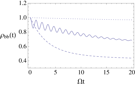
Figure 2: The occupation of the spin up state as a function of time in the case of magnetic leads. $\Gamma_{4}/\Omega=0.04$, $\Gamma_{3}=0$, $\Gamma_{2}/\Omega=0.08$, $\Gamma_{1}=0$ and $\delta/\Omega=5$. The curves correspond to different values of the $\gamma$ parameter: $\gamma=0$ (solid), $\gamma/8=10\Omega$ (dashed), and $\gamma/8=10^{3}\Omega$ (dotted).

This is a direct consequence of the conditions imposed, which result that the state $|b\,\rangle$ is the preferred steady-state due to the combination of right lead magnetization and the direction of tunneling.
 While for small $t$ the transition is slowed down, after some critical time $t>t_{0}$ an enhanced decay can be seen (Figs. 2) for $\gamma$ values comparable to the energy level displacement $\delta$. This enhanced decay results faster transition between the spin up and the spin down states than in the unmeasured system. Nevertheless the effect is just the opposite of the QZE. These behaviours are also reflected in the steady-state. If the enhanced decay occur then the probability of the state $|b\,\rangle$ is smaller than in the case of the unmeasured system.
 In spite of great progress made in microfabrication techniques, the construction of magnetic leads to a tiny quantum dot is still a challenge and we also study the considered system with normal leads. The localization into the state $|b\,\rangle$ as in the magnetic lead model is impossible, because both the spin up and spin down states can be filled from left and emptied to right. Examining the results in Figs. 3 the effect of suppressed transition can be found for small values of $t$. Here, the system cannot be frozen in its initial state as a consequence of the normal leads. When $\gamma$ is comparable with $\delta$ then the effect of the enhanced decay characterize the time evolution of the state $|b\,\rangle$. The steady-state behaviour shows a different aspect than in the case of magnetic leads. If the strength of the measurement increases then the probability of the state $|b\,\rangle$ is increasing. In the case of the unmeasured system, the probability of the steady state $|b\,\rangle$ may decrease as a function of $\delta$, but for large values of $\gamma$ is an increasing function of $\delta$. This means, when the suppression of the coherent oscillations is weak and the energy difference $\delta$ is large enough, then the probability of filling up the state $|b\,\rangle$ is less likely. As we expect, the probability of the steady state $|c\,\rangle$, the lower energy level, has the opposite character as a function of $\gamma$. These behaviours are shown in Fig. 4. Here, exists a mixed state, namely $\lim_{\gamma\to\infty}\hat{\rho}(t\to\infty)$, which provides the QZE. If this state can be prepared as an initial condition, then for the case of no magnetization measurement the system evolves into another mixed state, but for infinite accuracy measurement $\Delta M\to 0$ (eq. (8)), $\gamma\to\infty$, the system remains frozen in its initial condition.
 Next we analyze the electric current flowing through the system. This quantity is the only measurement result retained and we study it, to show the presence of measurement back-action. Using eqs. (2), (32) we obtain the average electric current [28]:

$$\langle{\Psi(t)}|\hat{I}|{\Psi(t)}\rangle=e\Big{(}\Gamma_{3}\sum_{n}\rho^{(n)}_{bb}(t)+\Gamma_{4}\sum_{n}\rho^{(n)}_{cc}(t)$$

$$+2\sqrt{\Gamma_{3}\Gamma_{4}}\sum_{n}\mathrm{Re}[\rho^{(n)}_{bc}(t)]+(\Gamma_{1}+\Gamma_{2})\sum_{n}\rho^{(n)}_{dd}(t)\Big{)}.$$

Figure 3: The occupation of the spin up state as a function of time in the case of normal leads. $\Gamma_{4}/\Omega=0.04$, $\Gamma_{3}/\Omega=0.06$, $\Gamma_{2}/\Omega=0.08$, $\Gamma_{1}/\Omega=0.1$ and $\delta/\Omega=5$. The curves correspond to different values of the $\gamma$ parameter: $\gamma=0$ (solid), $\gamma/8=10\Omega$ (dashed), and $\gamma/8=10^{3}\Omega$ (dotted).

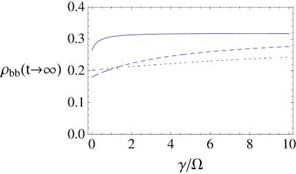
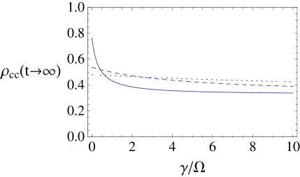
Figure 4: Probability of the $|b\,\rangle$(spin up) and $|c\,\rangle$(spin down) steady states as a function of the rescaled damping parameter. $\Gamma_{1}/\Omega=0.1$, $\Gamma_{2}/\Omega=0.08$, $\Gamma_{3}/\Omega=0.06$ and $\Gamma_{4}/\Omega=0.04$. The curves correspond to different values of the rescaled energy difference: $\delta/\Omega=1$ (solid), $\delta/\Omega=5$ (dashed), and $\delta/\Omega=10$ (dotted).

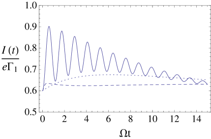
Figure 5: Electron current through the dot as a function of time. $\Gamma_{4}/\Omega=0.04$, $\Gamma_{3}/\Omega=0.06$, $\Gamma_{2}/\Omega=0.08$, $\Gamma_{1}/\Omega=0.1$ and $\delta/\Omega=5$. The curves correspond to different values of the $\gamma$ parameter: $\gamma=0$ (solid), $\gamma/8=10\Omega$ (dashed), and $\gamma/8=10^{3}\Omega$ (dotted).

In Fig. 5 we find the suppression effect induced by the continuous measurement. In the case of no measurement the current is increasing and oscillating and then is followed by a decrease and relaxation to the steady-state. If the enhanced decay occur in the spin up state then the current shows a slow increase and a quick relaxation to its stationary value, which is bigger than the value found for the unmeasured case. If the measurement is extremely strong then the current is increasing slowly compared to the other cases, the relaxation is longer and the asymptotic value is the highest. This means that the suppression of transitions can be determined directly after a short time evolution of the system or indirectly by examining the relaxation mechanism. The electric current in the magnetic leads case is zero, when QZE occurs.
 In a future experimental setup where this double detection setup will be applied, changing the conditions of the unsharp detection and analyzing the sharp detection output, the scope of the continuous quantum measurement theory may be demonstrated. The substrate induced decoherence was treated, so a possible charge current change will only be the result of a measurement back-action.

4 The accuracy of the measurement

We analyzed the detection of measurement back-action by the average electric current, which can be determined from ensemble measurements. The latter involves the problem of accuracy. If the current can be detected directly, via its magnetic field [29], then the states of the dot can be monitored with any accuracy.
 If such a measurement cannot be performed, one can make an indirect measurement. Obtaining the charge counting statistics in the right lead is the most plausible in this systems and from the statistics can be deduced the average current. Recently, there was another suggestion, where the variation of the right lead charge was discussed [30]. In this cases the standard deviation $\sigma_{\hat{I}}$ of the electric current from its mean can be best understood from the uncertainty principle. The uncertainty principle gives a lower bound for the standard deviation. The upper bound of the standard deviation is the square root of the second moment. The standard deviation could be any number between these bounds. However, we focus on the lower bound, because this quantity tells us when the measurement of the current could be less uncertain.
 For the observables $\hat{I},\hat{N}$ and the pure state $|{\Psi}\rangle$ the following inequality holds:

$$\sigma^{2}_{\hat{I}}\sigma^{2}_{\hat{N}}\geq\frac{1}{4}\Big{|}\langle{\Psi}|\left[\hat{I},\hat{N}\right]|{\Psi}\rangle\Big{|}^{2},$$ (34)

where (see [28])

$$\sigma^{2}_{\hat{I}} = \langle{\Psi}|\hat{I}^{2}|{\Psi}\rangle-\langle{\Psi}|\hat{I}|{\Psi}\rangle^{2},$$ (35)

$$\sigma^{2}_{\hat{N}} = \langle{\Psi}|\hat{N}^{2}|{\Psi}\rangle-\langle{\Psi}|\hat{N}|{\Psi}\rangle^{2}.$$ (36)

We calculate the right hand side of the inequality by using the eqs. (2),(32):

$$\left[\hat{I},\hat{N}\right]=i\,e\,\sum_{r,s}\left(\omega^{*}_{r,s}\hat{a}^{\dagger}_{D,s}\hat{a}_{r,s}+\omega_{r,s}\hat{a}^{\dagger}_{r,s}\hat{a}_{D,s}\right),$$ (37)

$$\langle{\Psi}|\left[\hat{I},\hat{N}\right]|{\Psi}\rangle=-2i\,e\sqrt{\Gamma_{3}\Gamma_{4}}\sum_{n}\mathrm{Im}[\rho^{(n)}_{bc}(t)]$$

$$=-2i\,e\sqrt{\Gamma_{3}\Gamma_{4}}\mathrm{Im}[\rho_{bc}(t)].$$ (38)

In order to evaluate the standard deviation of the charge number, we have to rewrite the related averages in the following way

$$\langle{\Psi}|\hat{N}|{\Psi}\rangle = \overline{n}_{aa}+\overline{n}_{bb}+\overline{n}_{cc}+\overline{n}_{dd},$$ (39)

$$\langle{\Psi}|\hat{N}^{2}|{\Psi}\rangle = \overline{n^{2}}_{aa}+\overline{n^{2}}_{bb}+\overline{n^{2}}_{cc}+\overline{n^{2}}_{dd}.$$ (40)

These new averages are defined as $\overline{n}_{ij}=\sum_{n}n\rho^{(n)}_{ij}$ and $\overline{n^{2}}_{ij}=\sum_{n}n^{2}\rho^{(n)}_{ij}$. Multiply eqs. (22), (23), (24), (25), (26) by $n$ or $n^{2}$ and sum over $n$ one finds coupled differential equations

$$\dot{\rho}_{aa} = -(\Gamma_{1}+\Gamma_{2})\rho_{aa}+\Gamma_{3}\rho_{bb}+\Gamma_{4}\rho_{cc}$$ (41)

$$+ \sqrt{\Gamma_{3}\Gamma_{4}}(\rho_{bc}+\rho_{cb}),$$

$$\dot{\overline{n}}_{aa} = -(\Gamma_{1}+\Gamma_{2})\overline{n}_{aa}+\Gamma_{3}\overline{n}_{bb}+\Gamma_{4}\overline{n}_{cc}$$ (42)

$$+ \sqrt{\Gamma_{3}\Gamma_{4}}(\overline{n}_{bc}+\overline{n}_{cb})+\Gamma_{3}\rho_{bb}+\Gamma_{4}\rho_{cc}$$

$$+ \sqrt{\Gamma_{3}\Gamma_{4}}(\rho_{bc}+\rho_{cb}),$$

$$\dot{\overline{n^{2}}}_{aa} = (\Gamma_{1}+\Gamma_{2})\overline{n^{2}}_{aa}+\Gamma_{3}\overline{n^{2}}_{bb}+\Gamma_{4}\overline{n^{2}}_{cc}$$ (43)

$$+ \sqrt{\Gamma_{3}\Gamma_{4}}(\overline{n^{2}}_{bc}+\overline{n^{2}}_{cb})+2\Gamma_{3}\overline{n}_{bb}+2\Gamma_{4}\overline{n}_{cc}$$

$$+ 2\sqrt{\Gamma_{3}\Gamma_{4}}(\overline{n}_{bc}+\overline{n}_{cb})+\Gamma_{3}\rho_{bb}+\Gamma_{4}\rho_{cc}$$

$$+ \sqrt{\Gamma_{3}\Gamma_{4}}(\rho_{bc}+\rho_{cb}),$$

$$\ldots$$

where $\rho_{ij}=\sum_{n}\rho^{(n)}_{ij}$. We rewrite eq. (34) as

$$\sigma_{\hat{I}}\geq\frac{e\sqrt{\Gamma_{3}\Gamma_{4}}\Big{|}\mathrm{Im}[\rho_{bc}(t)]\Big{|}}{\sqrt{\sum_{i}\overline{n^{2}}_{ii}(t)-\Big{(}\sum_{i}\overline{n}_{ii}(t)\Big{)}^{2}}},\,\,i\in\{a,b,c,d\},$$ (44)

where the right hand side of the inequality is given by the coupled differential equations found above.

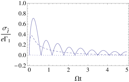
Figure 6: The lower bounds of the standard deviation (electric current) as a function of time. $\Gamma_{4}/\Omega=0.04$, $\Gamma_{3}/\Omega=0.06$, $\Gamma_{2}/\Omega=0.08$, $\Gamma_{1}/\Omega=0.1$ and $\delta/\Omega=5$. The curves correspond to different values of the $\gamma$ parameter: $\gamma=0$ (solid), $\gamma/8=10\Omega$ (dashed), and $\gamma/8=10^{3}\Omega$ (dotted).

We consider that the system is initially in the spin up state. Figs. 6 shows that the standard deviation of the electric current is decreased in time. However, the effect in interest, induced by the continuous measurement, takes place for short times. Figs. 6 also shows that in the case of $\gamma/8\gg\Omega$, the lowest possible value of $\sigma_{\hat{I}}$ is small for short times. This is not surprising(see eq. (44)) since the large decoherence generated by the magnetization detector, reduces the off-diagonal elements to zero. It follows from our analysis that only highly accurate measurement cases (see eq. (8)) could have small standard deviations. Having two different setup with $\gamma$ and $\gamma^{\prime}$ parameters and implementing the $\gamma,\gamma^{\prime}\gg\Omega$ condition, the rate of the suppression can also be compared.

5 Conclusions

In this paper we considered a simple spin-dependent quantum dot and we studied the mechanism of continuous magnetization measurement by a detected electric current. Starting with the many-particle wave function in the occupation number representation and adding the dynamics of the continuous measurement, we have found the equations of motion for the system. Our derivation contains an important assumption, namely that the energy states of the system are deep inside the bias $\mu_{l}-\mu_{r}$. If this condition is not fulfilled, then more off-diagonal elements may appear in the equation of motion, and new couplings between different density matrix elements may occur. The continuous measurement of the magnetization induce a damping rate in the equations for the off-diagonal density-matrix elements. The analysis revealed that the states of the dot can be determined only by a electric current measurement, due to the spectral decomposition of the current operator.
 The back-action of the continuous detection damps the oscillations between the different spin states. We investigated the case of magnetic leads, where an enhanced decay takes place when the damping parameter $\gamma$ is comparable with the energy level displacement $\delta$. The spin up state is the preferred steady-state as the consequence of our choice of lead magnetization and the tunneling direction. If this state is the initial state of the system, then for very strong measurements the system remains frozen there, showing the presence of quantum Zeno effect. We found that the damping mechanism in the case of normal leads is also suppressing the coherent motion and inducing an enhanced decay, too. Here, the spin up state is no more a preferred steady-state and for strong measurements the system tends to a particular mixed state. The behaviour of the enhanced decay and the strong damping is reflected also in the steady-state of the system. When the enhanced decay occurs the steady-state values are smaller (state $|b\,\rangle$) or higher (state $|c\,\rangle$) than in the case of the unmeasured system. If $\gamma/8<\delta$, then there is a faster increase in the steady-state $|b\,\rangle$ as a function of $\gamma/\Omega$.
 We studied the electric current as the only quantity retained by the detector. The increase rate of the electric current for short times depends inversely proportional on the continuous measurement parameter $\gamma$. If the parameter $\gamma$ increase, the rate of the current is decreasing. The current shows a quick relaxation to its stationary value, when the enhanced decay occurs in the spin states. In the case of strong damping, a long relaxation characterize the time evolution of the electric current. The results also show that the coherent oscillations die out for $\gamma/\Omega\gg 1$. When quantum Zeno effect occurs in the case of magnetic leads, then the electric current is zero.
 In a real experiment the mean value of the electric current is deduced form the charge counting statistics. This shows a necessity of studying the standard deviation of the electric current from its mean. We derived a lower bound for the deviation, using the Heisenberg uncertainty principle. We found that only for highly accurate magnetization measurements is possible to analyze measurement back-action and quantum Zeno effect by the detection of the electric current.
 Experimentally, the analyzed model can be implemented by semiconductor spin-light emitting diode structures containing single layers of InAs/GaAs self-assembled quantum dots [3]. Application of a oblique magnetic field ($\overrightarrow{B}(B_{x},0,B_{z})$ in the model) results the emission of a circular polarized light [31]. The emitted light is used for measuring the polarization of the injected spin or the spin dynamics in the quantum dot [32]. The photon detector in these experiments is the apparatus, which we modeled as the unsharp detector in the theory presented. The applied oblique magnetic field is 40-50 mT, which results a Larmor frequency $\Omega=g\mu_{B}B/\hbar\sim 10^{8}s^{-1}$, where $g$ is the effective Landé factor and $\mu_{B}$ is the Bohr magneton. The characteristic time of a tunneling process is $\tau\sim\mu s-ms$ and a typical tunneling rate $\Gamma\sim 10^{3}-10^{6}s^{-1}$. The time scale of the inverse measurement parameter $1/\gamma$ and of the photon emission process can be taken to be the same. The emission time $\tau\sim ns$ and then $\gamma\sim 10^{9}s^{-1}$. $\gamma$ depends on the accuracy and the bandwidth of the photon detector, so $10^{9}s^{-1}$ should be considered as the lower bound for this parameter. These parameters are adjustable, so the requirements of our analysis might be achieved by a real experimental setup. There are other decoherence sources in these devices, as hyperfine interactions with unpolarized nuclei, the temperature dependent phonon absorption and emission. These decoherences are competing with the measurement induced decoherence. However, their decoherence rate cannot be manipulated at will, so the effects induced by the adjustable $\gamma$ should be filtered out by a series of measurements.
 The model offers some insight into the measurement induced back-action and studies the way the QZE appears in a complex system. An experimental study has the potential to analyze the scope of the continuous quantum measurement theory in mesoscopic solid state physics. Tight control of systems parameters may strongly enhance the possibilities of observing the measurement-induced back-action.

The author would like to thank S. A. Gurvitz for discussions and encouragement. J. Z. B. has profited also from helpful suggestions made by T. Geszti, M. Jääskeläinen, and U. Zülicke. This work was supported by a postdoctoral fellowship grant from the Massey University Research Fund. Additional funding through BMBF project QK_QuOReP is gratefully acknowledged.

Appendix A General measurements

Usually the von Neumann measurement that is discussed, when the system is projected onto one of the possible eigenstates of a given observable. Considering these eigenstates as $\{|n\rangle:n=1,\ldots,d\}$ and the state of the system $|\psi\rangle=\sum_{n}a_{n}|n\rangle$, then the system is randomly projected onto $|n\rangle$ with the probability $p_{n}=|a_{n}|^{2}$. The properties of the projectors are:

$$\sum_{n}\hat{P}_{n} = \hat{I},$$ (45)

$$\hat{P}_{n}\hat{P}_{n} = \delta_{n,m}\hat{P}_{n}.$$ (46)

These sharp measurements can be discussed in two ways. Selective case is when the system is randomly projected onto an eigenstate

$$\hat{\rho} \rightarrow \hat{\rho}_{n}=\frac{\hat{P}_{n}\hat{\rho}\hat{P}_{n}}{\mathrm{Tr}[\hat{P}_{n}\hat{\rho}\hat{P}_{n}]},$$ (47)

$$\hat{A} \rightarrow A_{n},$$ (48)

where the possibility to detect eigenvalue $A_{n}$ is $p_{n}=\mathrm{Tr}[\hat{P}_{n}\hat{\rho}\hat{P}_{n}]$.
Nonselective description represent a measurement scenario, where our record of the result $A_{n}$ was lost. We have a quantum system in the state $\hat{\rho}_{n}$ with probability $p_{n}$, but we no longer know the actual value of $A_{n}$. The state of such a quantum system is the mixture of the states $\hat{\rho}_{n}$ with probabilities $p_{n}$. Due to the rules of probability theory, the following results are obtained:

$$\hat{\rho} \rightarrow \hat{\rho}_{n}=\sum_{n}p_{n}\hat{\rho}_{n}=\sum_{n}\hat{P}_{n}\hat{\rho}\hat{P}_{n},$$ (49)

$$\hat{A} \rightarrow \sum_{n}p_{n}A_{n}=\langle\hat{A}\rangle.$$ (50)

A von Neumann measurement provides complete information and the system is always projected into an eigenstate. However, there exist many measurements, which are unable to detect sharply these eigenvalues. If the detector plus the system is under a projective measurement scenario, then the larger system will act on the system in ways that cannot be described by projective measurement on the system alone. For these purposes we need to consider a general class of measurements, which result reduced quantity of information about an observable.

These unsharp measurements can be described by generalizing the set of projectors. The construction can be done in two ways: the cardinality of the sets are countable or infinite. Suppose we pick a set of $N$ operators $\hat{\Pi}_{n}$, the restrictions are: $\sum_{n=1}^{N}\hat{\Pi}_{n}=\hat{I}$, where $\hat{I}$ is the identity operator and $\hat{\Pi}_{n}$ to be hermitian positive semidefinite. A hermitian positive semidefinite operator can always be written as, $\hat{\Pi}_{n}=\hat{M}^{\dagger}_{n}\hat{M}_{n}$, for some operator $\hat{M}_{n}$. If the positivity of $\hat{M}_{n}$ is not required, the square root of $\hat{\Pi}_{n}$ can give infinite solutions, which means that there are infinite different experimental apparatuses that gives the same probabilities for the outcomes.
The selective description is:

$$\hat{\rho}\rightarrow\hat{\rho}_{n}=\frac{\hat{M}_{n}\hat{\rho}\hat{M}^{\dagger}_{n}}{\mathrm{Tr}[\hat{M}_{n}\hat{\rho}\hat{M}^{\dagger}_{n}]},$$ (51)

with

$$p_{n} = \mathrm{Tr}[\hat{M}_{n}\hat{\rho}\hat{M}^{\dagger}_{n}],$$ (52)

$$\sum_{n=1}^{N}p_{n} = 1,$$ (53)

giving the probability of obtaining the $n$th outcome.
The nonselective description is:

$$\hat{\rho}\rightarrow\sum_{n=1}^{N}p_{n}\hat{\rho}_{n}=\sum_{n=1}^{N}\hat{M}_{n}\hat{\rho}\hat{M}^{\dagger}_{n}.$$ (54)

The set can be countable infinite, here we have $N=\infty$, but also uncountable infinite is possible where the sum will be replaced by an integral and the normalization is:

$$\int p(x)dx=1.$$ (55)

These generalized measurements are called as POVM’s (positive operator-valued measure). The mappings of the density matrices in eqs. (49), (54) has a specific form, called Kraus-form [5].

Appendix B Continuous quantum measurement of an observable

A continuous measurement is referring to a scenario, where the measurement data is continually extracted from a system. In order to construct a measurement like this, we consider the partition of the time line into a sequence of intervals of length $\Delta t$, and consider an unsharp measurement in each interval. In this construction, there is a mathematical requirement for obtaining a dynamical equations, namely the strength of each measurement must depend on the length of the time interval. This construction circumvent the problem of instantaneous effect of a standard quantum measurement.

We now divide time into intervals of length $\Delta t$. In each time interval, we will make a measurement described by the operators

$$\hat{\Pi}(x)=\frac{1}{\sqrt{2\pi\sigma^{2}}}\mathrm{exp}\left[-\frac{(x-\hat{A})^{2}}{2\sigma^{2}}\right],\,\,-\infty\leqslant x\leqslant\infty.$$ (56)

Each operator $\hat{\Pi}(x)$ a Gaussian-weighted sum of projectors onto the eigenstates of $\hat{A}$ and the probability

$$p(x)=\mathrm{Tr}\left(\hat{\Pi}(x)\hat{\rho}\right),\,\,\int p(x)dx=1.$$ (57)

The observable $\hat{A}$ can be any kind of Hermitian operator. The following equation is also true:

$$\langle x\rangle=\int xp(x)dx=\langle\hat{A}\rangle.$$ (58)

The strength of the continuous measurement is $\gamma$ defined by

$$\gamma=\frac{1}{\Delta t\,\sigma^{2}}.$$ (59)

The selective description of such a measurement (eq. (56)) is derived by introducing $x$ as a stochastic quantity. Main reason for this is to keep the random nature of the measurement and due to eq. (58) we can write:

$$x(t+\Delta t)-x(t)=\langle\hat{A}\rangle\,\Delta t+\frac{W_{t+\Delta t}-W_{t}}{\sqrt{\gamma}},$$ (60)

where $W$ is the Wiener process, a Gaussian random variable. The measurement result gives the average value $\hat{A}$ in the time interval $\Delta t$ but also a random value due to the form of $\hat{\Pi}(x)$.

Now, we make a sequence form the aforementioned measurements and take the limit $\Delta t\rightarrow 0$. As the limit is taken, then $\hat{\Pi}(\Delta t\to 0)\to 0$ in eq. (56). To derive a dynamical equation, it is enough to consider the change induced by operator $\hat{\Pi}(x)$, since the operator is the function of $\Delta t$ and does not change during the time interval $t$. The measurement induced change is derived to the first order in $\Delta t$. The state after the measurement yields

$$|\Psi(t+\Delta t)\rangle=\frac{1}{\sqrt{p(x)}}\hat{\Pi}(x)^{1/2}|\Psi(t)\rangle.$$ (61)

Expanding $\hat{\Pi}(x)^{1/2}$ to first order in $\Delta t$, leads to the relation

$$\mid\Psi(t+\Delta t)\rangle\varpropto\left[1-\frac{\gamma}{8}\left(\langle\hat{A}\rangle-\hat{A}\right)^{2}\Delta t-\frac{\sqrt{\gamma}}{2}\left(\langle\hat{A}\rangle-\hat{A}\right)\Delta W\right]\mid\Psi(t)\rangle,$$ (62)

where we used that in the limit of $\Delta t\rightarrow 0$, $(\Delta W)^{2}\rightarrow\Delta t$. These equation does not preserve the norm of the wave function, so we have to calculate $p(x)$ in the first order expansion in $\Delta t$, including the stochastic calculation rule induced above. Now we take the limit $\Delta t\rightarrow 0$, setting $\Delta t=dt$, $\Delta W=dW$ and $(\Delta W)^{2}=dt$ we get

$$|\Psi(t+\Delta t)\rangle=|\Psi(t)\rangle+d|\Psi\rangle,$$ (63)

$$d|\Psi\rangle=\left[-\frac{\gamma}{8}\left(\langle\hat{A}\rangle-\hat{A}\right)^{2}dt-\frac{\sqrt{\gamma}}{2}\left(\langle\hat{A}\rangle-\hat{A}\right)dW\right]|\Psi\rangle.$$

This is the equation which describes the evolution of the state of a system in a time interval $dt$ and it is called stochastic Schrödinger equation. The state $|\psi\rangle$ evolves randomly. An equation for the density operator $\hat{\rho}$ can be derived, too. Using the same stochastic calculation rules, and defining $\hat{\rho}(t+dt)=\hat{\rho}(t)+d\hat{\rho}$, we have

$$d\hat{\rho}=-\frac{\gamma}{8}\left[\hat{A},\left[\hat{A},\hat{\rho}\right]\right]dt+\frac{\sqrt{\gamma}}{2}\left(\hat{A}\hat{\rho}+\hat{\rho}\hat{A}-2\langle\hat{A}\rangle\hat{\rho}\right)dW,$$ (64)

a stochastic master equation.

The nonselective description is when the observer makes the continuous measurement, but throws away the information regarding the measurement results, i.e detecting the average of an observable instead of the eigenvalues, so the observer must average over the different possible results. Due to the construction of the model the quantities $\rho$ and $dW$ are statistically independent, $\ll\rho\,dW\gg=0$ (average over all possible realizations and over the Hilbert space states). Thereby, we can set to zero all terms proportional to $dW$ in eq. (64), which yields

$$\frac{d\hat{\rho}}{dt}=-\frac{\gamma}{8}\left[\hat{A},\left[\hat{A},\hat{\rho}\right]\right].$$ (65)

The double-commutator describes the decoherence caused by the continuous quantum measurement.
Eq. (65) also can be achieved without introducing the random variables. For a time interval $\Delta t$ the nonselective evolution of the density matrix is

$$\hat{\rho}(t+\Delta t)=\int\hat{\Pi}(x)^{1/2}\hat{\rho}(t)\hat{\Pi}(x)^{1/2}dx.$$ (66)

Expanding this equation into series up to the leading term $\Delta t$ and calculating the integral, the following result can be obtained

$$\hat{\rho}(t+\Delta t)=\hat{\rho}(t)-\frac{\gamma}{8}\Big{(}\hat{A}^{2}\hat{\rho}(t)-2\hat{A}\hat{\rho}(t)\hat{A}+\hat{\rho}(t)\hat{A}^{2}\Big{)}\Delta t.$$ (67)

Taking the limit $\Delta t\rightarrow 0$ we arrive at the same equation as eq. (65).

Under unitary evolution, the following transformation is added to eq. (63)

$$|\psi\rangle\rightarrow|\psi\rangle+d|\psi\rangle=\left(1-i\frac{\hat{H}}{\hbar}\,dt\right)|\psi\rangle,$$ (68)

where $\hat{H}$ is the Hamiltonian. For the eqs. (64),(65) the transformation is:

$$\hat{\rho}+d\hat{\rho}=\hat{\rho}-\frac{i}{\hbar}[\hat{H},\hat{\rho}]\,dt.$$ (69)

If we want to treat non-unitary dynamics then the infinitesimal transformation $\mathcal{L}\hat{\rho}\,dt$ can be added only to eqs. (64) and (65). We have to remark also that the form of the equation of motion, namely the appearance of the double commutator, is the consequence of the Gaussian form of $\hat{\Pi}(x)$.

References

- [1] B. Misra, and E. C. G. Sudarshan, J. Math. Phys. 18, 756 (1977).
- [2] L. I. Mandelstam, Lectures on Optics, the Theory of Relativity, and Quantum Mechanics (Nauka, Moscow, 1972)
- [3] G. Itskos, E. Harbord, S. K. Clowes, E. Clarke, L. F. Cohen, R. Murray, P. Van Dorpe, and W. Van Roy, Appl. Phys. Lett. 88, 022113 (2006).
- [4] H.-P. Breuer and F. Petruccione, The theory of open quantum systems (Oxford University Press, Oxford 2002)
- [5] K. Kraus, States, Effects, and Operations: Fundamental Notions of Quantum Theory (Springer, Berlin Heidelberg New York, 1983)
- [6] The effects of the ever-present environmental nuclear magnetic field can be interpreted as an unsharp measurement, however this cannot be manipulated at will.
- [7] K. Jacobs, and D.A. Steck, Contemp.Phys. 47, 279 (2006); L. Diósi, in: J.-P. Françoise, G. L. Naber, and S. T. Tsou (eds), Encyclopedia of Mathematical Physics, vol. 4 (Academic Press, Oxford, 2006), p. 276.
- [8] J. M. Elzerman, R. Hanson, L. H. Willems van Beveren, B. Witkamp, L. M. K. Vandersypen, and L. P. Kouwenhoven, Nature 430, 431 (2004).
- [9] S. D. Barrett, and T. M. Stace, Phys. Rev. B 73, 075324 (2006).
- [10] B. E. Kane, Nature 393, 133 (1998).
- [11] D. Loss and D. P. DiVincenzo, Phys. Rev. A 57, 120 (1998); A. V. Khaetskii, D. Loss and L. Glazman, Phys. Rev. Lett. 88, 186802 (2002); H.-A. Engel and D. Loss, Phys. Rev. B. 65, 195321 (2002).
- [12] F. Jelezko, T. Gaebel, I. Popa, A. Gruber, and J. Wrachtrup, Phys. Rev. Lett. 92, 076401 (2004).
- [13] S. A. Gurvitz, Phys. Rev. B 56, 15215 (1997).
- [14] A. N. Korotkov, Phys. Rev. B 60, 5737 (1999); 63, 115403 (2001).
- [15] H.-S. Goan and G.J.Milburn, Phys. Rev. B 64, 235307 (2001).
- [16] W. Mao, D. V. Averin, R. Ruskov, and A. N. Korotkov, Phys. Rev. Lett. 93, 056803 (2004); S. Gustavsson, R. Leturcq, B. Simovic, R. Schleser, T. Ihn, P. Studerus, K. Ensslin, D. C. Driscoll, and A. C. Gossard, Phys. Rev. Lett. 96, 076605 (2006); R. Ruskov, A. N. Korotkov and A. Mizel, Phys. Rev. Lett. 96, 200404 (2006); T. Geszti and J. Z. Bernad, Phys. Rev. B 73, 235343 (2006); T. Gilad and S. A. Gurvitz, Phys. Rev. Lett. 97, 116806 (2006); L. Tian, Phys. Rev. Lett. 98, 153602 (2007); C. Hines, K. Jacobs, and J. B. Wang, J. Phys. A: Math. Theor. 40, F609 (2007); N. P. Oxtoby, J. Gambetta, and H. M. Wiseman, Phys. Rev. B 77, 125304 (2008).
- [17] G. Hackenbroich, B. Rosenow, and H. A. Weidenmuller, Phys. Rev. Lett. 81, 5896 (1998); S. A. Gurvitz, L. Fedichkin, D. Mozyrsky, and G. P. Berman, Phys. Rev. Lett. 91, 066801 (2003); T. M. Stace and S. D. Barrett, Phys. Rev. Lett. 92, 136802 (2004); 94, 069702 (2005); A. A. Clerk and A. D. Stone, Phys. Rev. B 69, 245303 (2004); D. V. Averin and A. N. Korotkov, Phys. Rev. Lett. 94, 069701 (2005).
- [18] J. Z. Bernád, A. Bodor, T. Geszti, and L. Diósi, Phys. Rev. B 77, 073311 (2008).
- [19] L. Diósi, A Short Course in Quantum Information Theory: An Approach from Theoretical Physics, Lect. Notes Phys. 713, (Spinger, Berlin 2007).
- [20] M. A. Nielsen and I. L. Chuang, Quantum Computation and Quantum Information (Cambridge University, Cambridge, 2000)
- [21] F. H. L. Koppens, J. A. Folk, J. M. Elzerman, R. Hanson, L. H. Willems van Beveren, I. T. Vink, H. P. Tranitz, W. Wegscheider, L. P. Kouwenhoven, and L. M. K. Vandersypen, Science 309, 1346 (2005).
- [22] J. R. Petta, A. C. Johnson, J. M. Taylor, E. A. Laird, A. Yacoby, M. D. Lukin, C. M. Marcus, M. P. Hanson, and A. C. Gossard, Science 309, 2180 (2005).
- [23] R. L. Hudson and K. R. Parthasarathy, Commun. Math. Phys. 93, 301 (1984).
- [24] J. Z. Bernád, M. Jääskeläinen, and U. Zülicke, Phys. Rev. B 81, 073403 (2010).
- [25] S. A. Gurvitz and Y. S. Prager, Phys. Rev. B. 53, 15932 (1996).
- [26] A. Barchielli, L. Lanz, and G. M. Prosperi, Nuovo Cimento 72 B, 79 (1982).
- [27] A. Barchielli, L. Lanz, and G. M. Prosperi, Found. Phys. 13, 779 (1983).
- [28] In the present formalism it takes some extra care to calculate . This average is not only the quantum mechanical average of an operator, but an average over the random variable, too. Here, the random variable is the standard Wiener process. The need of a double average is generated by the condition.
- [29] L. S. Levitov, H. Lee, and G. B. Lesovik, J. Math. Phys. 37, 4845 (1996).
- [30] S. A. Gurvitz, Int. J. of Mod. Phys. B 20, 1363 (2006).
- [31] M. I. Dykonov and V. I. Perel, in Optical Orientation, edited by F. Meier and B. P. Zakharchenya (͑North Holland, Amsterdam, 1984͒), pp. 11–50.
- [32] V. F. Motsnyi, P. Van Dorpe, W. Van Roy, E. Goovaerts, V. I. Safarov, G. Borghs, and J. De Boeck, Phys. Rev. B 68, 245319 (2003).