Tests of the Standard Electroweak Model at the Energy Frontier

Abstract

In this review, we summarize tests of standard electroweak (EW) theory at the highest available energies as a precursor to the Large Hadron Collider (LHC) era. Our primary focus is on the published results (as of March 2010) from proton-antiproton collisions at $\sqrt{s}=1.96$ TeV at the Fermilab Tevatron collected using the CDF and D0 detectors. This review is very timely since the LHC scientific program is nearly underway with the first high-energy ($\sqrt{s}=7$ TeV) collisions about to begin. After presenting an overview of the EW sector of the standard model, we provide a summary of current experimental tests of EW theory. These include gauge boson properties and self-couplings, tests of EW physics from top quark sector, and searches for the Higgs boson.

I INTRODUCTION

The goal of particle physics is to explain the nature of the Universe at its most fundamental level, including the basic constituents of matter and their interactions. The standard model of particle physics (SM) is a quantum field theory based on the $SU(3)_{\rm C}\otimes SU(2)_{\rm L}\otimes U(1)_{Y}$ gauge symmetry group which describes the strong, weak, and electromagnetic interactions among fundamental particles. This theory has been the focus of intense scrutiny by experimental physicists, most notably at high energy particle colliders, over the last three decades. It has been demonstrated to accurately describe fundamental particles and their interactions up to $O(100)$ GeV, with the existence of non-zero neutrino masses and mixing being the only known exception. Despite the success of the SM, there are many reasons to believe that the SM is an effective theory which is only valid up to $\sim$1 TeV. Some of the shortcomings of the SM will be described in Section II.

Particle physics is embarking on a unique, and possibly defining, period in its history with the start of particle collisions at the Large Hadron Collider (LHC) at CERN. At the LHC, bunches of protons will be collided with a planned 14 TeV of center-of-mass energy, creating conditions that existed only a tiny fraction of a second after the big bang. This is seven times the center of mass energy of collisions at the Fermilab Tevatron. For the first time, physicists will be able to directly probe the TeV energy scale in the laboratory, where new physics beyond the SM, with the potential to revolutionize our understanding of the Universe, could be apparent. We can only speculate about what form this will take. Is is a tantalizing prospect that on the horizon is a revolution in our understanding of the Universe that includes a more complete theory of particles and their interactions which may explain dark matter and dark energy.

The purpose of this review is to present tests of the electroweak (EW) sector of the SM ($SU(2)_{\rm L}\otimes U(1)_{Y}$) at the highest available energies as a precursor to the LHC era. Our focus is on published results from collider data collected using the CDF [1] and D0 [2] detectors during Run II at the Fermilab Tevatron as it relates to our understanding of electroweak interactions and spontaneous symmetry breaking. After an overview of electroweak theory (Section II), we present current results on gauge boson properties and self-couplings (Section III), tests of electroweak physics from top quark physics (Section IV), and searches for the Higgs boson (Section V).

II OVERVIEW

The SM is an extremely successful theory of the strong, weak, and electromagnetic interactions. It is based on three generations of quarks and leptons, interacting via an $SU(3)_{\rm C}\otimes SU(2)_{\rm L}\otimes U(1)_{Y}$ gauge symmetry. The $SU(2)_{\rm L}\otimes U(1)_{Y}$ symmetry is spontaneously broken to electromagnetism, $U(1)_{EM}$, by the vacuum-expectation value of the Higgs field. Given this field content and gauge symmetry, the most general theory that follows from writing down every term of dimension four or less is the SM.

In the SM, as usually understood, neutrinos are exactly massless, and do not mix. Since neutrino mixing has been definitively observed, we must go beyond the SM in order to describe this phenomenon. There are two ways to do this. One way is to extend the field content of the model by adding additional fermion and/or Higgs fields (e.g. a right-handed neutrino or a Higgs triplet). The other way is to extend the SM by adding operators of dimensionality greater than four. There is only one operator of dimension five allowed by the gauge symmetries [3],

$${\cal L}_{5}=\frac{c^{ij}}{\Lambda}(L^{iT}\epsilon\phi)C(\phi^{T}\epsilon L^{j})+h.c.$$ (1)

where $L^{i}$ is the lepton doublet field of the $i^{th}$ generation and $\phi$ is the Higgs doublet field (the $2\times 2$ matrix $\epsilon$ and the $4\times 4$ charge-conjugation matrix $C$ are present to ensure invariance under $SU(2)_{\rm L}$ and Lorentz transformations, respectively). When the Higgs doublet acquires a vacuum-expectation value, $\langle\phi\rangle=(0,v/\sqrt{2})$ ($v=246$ GeV), this term gives rise to a (Majorana) mass for neutrinos,

$${\cal L}_{5}=-\frac{1}{2}M_{\nu}^{ij}\nu^{iT}C\nu^{j}+h.c.$$ (2)

where $M_{\nu}^{ij}=c^{ij}v^{2}/\Lambda$ is the neutrino mass matrix. Due to the tiny inferred masses of neutrinos, the scale $\Lambda$ lies around $10^{15}$ GeV, assuming $c^{ij}$ is not much less than order unity.

There are other indications that the SM is not a complete description of nature, most of them related to gravitation and cosmology. Even with massive neutrinos included, the SM particles only constitute 4.6% of the present universe, with the remainder in mysterious dark matter (23%) and dark energy (72%). Neither dark matter and nor dark energy are accommodated in the SM. There is no adequate mechanism for baryogenesis (the observed excess of baryons over antibaryons) or inflation, which is the simplest explanation of the observed temperature fluctuations in the cosmic microwave background. The SM also provides no explanation of the strong CP problem: the lack of observed CP violation in the strong interaction, which is allowed by the SM.

If physics beyond the SM lies at an energy scale less than 1 TeV, then we should be able to observe it directly at high-energy colliders. If it lies at a scale greater than 1 TeV, then we can parametrize its effects via higher-dimension operators, suppressed by inverse powers of the scale of new physics, $\Lambda$, exactly as in the case of neutrino masses described above. Other than the dimension-five operator responsible for neutrino masses, the lowest-dimension operators are of dimension six, and are therefore suppressed by two inverse powers of $\Lambda$. If $\Lambda$ is of order $10^{15}$ GeV, as suggested by neutrino masses, then these operators are so suppressed that they are unobservable, with the possible exception of baryon-number violating operators that mediate nucleon decay. However, there could be more than one scale of new physics, and if this scale is not much greater than 1 TeV, its effects could be observable via dimension six operators. Operators of dimension greater than six are suppressed by even more inverse powers of $\Lambda$ and can be neglected.

There are many dimension-six operators allowed by the SM gauge symmetry [4]. There are three ways to detect the presence of these operators. The first is to observe phenomena that are absolutely forbidden (or extremely suppressed) in the SM, such as nucleon decay. The second is to make measurements with such great precision that the small effects of the dimension-six operators manifest themselves. The third is to do experiments at such high energy, $E$, that the effects of these operators, of order $(E/\Lambda)^{2}$, become large. If $E>\Lambda$ then one must abandon this formalism, because operators of arbitrarily high dimensionality become significant; however, the new physics should then be directly observable. If no effects beyond the SM are observed, then one can place bounds on the coefficients of the dimension-six operators, $c/\Lambda^{2}$, where $c$ is a dimensionless number. These bounds apply only to the product $c/\Lambda^{2}$, not to $c$ and $\Lambda^{2}$ separately; in fact, there could even be two different scales of new physics involved ($\Lambda_{1}\Lambda_{2}$ in place of $\Lambda^{2}$).

This approach to physics beyond the SM, dubbed an effective-field-theory approach [3], has the advantage of being model independent. Whatever new physics lies at the scale $\Lambda$, it will induce dimension-six operators, whose only dependence on the new physics lies in their coefficients, $c/\Lambda^{2}$. Another advantage of this approach is that it is universal; it can be applied both to tree-level and loop-level processes, and any ultraviolet divergences that appear in loop processes can be absorbed into the coefficients of the operators. Thus one need not make any ad hoc assumptions about how the ultraviolet divergences are cut off. This effective-field-theory approach thus provides an excellent framework to parametrize physics beyond the SM [5; 6].

Hadron colliders contribute to the study of the electroweak interactions in three distinct ways. Firstly, because they operate at the energy frontier, hadron colliders are uniquely suited to searching for the effects of dimension six operators that are suppressed by a factor of $(E/\Lambda)^{2}$. Secondly, they are able to contribute to the precision measurement of a variety of electroweak processes, most notably to the measurement of the $W$ boson mass and the top quark mass. Thirdly, they are able to search for new particles associated with the electroweak interactions, in particular the Higgs boson. These three virtues of hadron colliders will manifest themselves throughout this review.

II.1 Electroweak Interactions

The electroweak theory is a spontaneously broken gauge theory based on the gauge group $SU(2)_{\rm L}\otimes U(1)_{Y}$. There are three parameters that describe the theory: the gauge couplings $g$ and $g^{\prime}$, and the order parameter of spontaneous symmetry breaking, $v$. In the SM, this order parameter is the vacuum expectation value of a fundamental Higgs field. These parameters are not measured directly, but rather inferred from precision electroweak measurements. The three measurements that are used to fix these parameters are the Fermi constant $G_{F}$ determined from the muon lifetime formula; the fine structure constant $\alpha$, determined from a variety of low-energy experiments; and the $Z$ boson mass $M_{Z}$. With these three inputs, the predictions of all other electroweak processes can be calculated, at least at tree level.

The level of precision of electroweak measurements is such that a tree-level analysis is insufficient, and one must go to at least one loop. At this level, one finds that predictions depend also on the top quark mass and the Higgs boson mass, since these particles appear in loops. In fact, a range for the top quark mass was correctly predicted by precision electroweak data before the top quark was discovered, and the measured mass falls into this range. We are now following the same tack with the Higgs boson. Remarkably, the precision electroweak data imply that the Higgs boson mass is not far above the experimental lower bound of $m_{H}>114~{}{\rm GeV/c}^{2}$, which means that it may be accessible at the Tevatron as well as the LHC.

The electroweak interaction has many other parameters as well. Along with the top quark mass, there are the masses of all the other quarks and leptons, as well as the elements of the Cabbibo-Kobayashi-Maskawa (CKM) quark-mixing matrix and the Maki-Nakagawa-Sakata (MNS) lepton-mixing matrix. Most of these mixing parameters are not measured at the energy frontier, with one exception: the CKM element $V_{tb}$ that describes the coupling of a $W$ boson to a top and bottom quark. The only direct measurement of this parameter comes from electroweak production of the top quark at hadron colliders via a process known as single-top production, discussed in Section IV.3.

II.2 Electroweak Symmetry Breaking

The strong and electroweak forces are gauge theories, based on the groups $SU(3)_{C}$ and $U(1)_{EM}$, respectively. The associated gauge bosons, the gluon and the photon, are massless as a consequence of the gauge symmetry. We know that the interactions of electroweak bosons with fermions as well as with themselves are also governed by a gauge theory, with gauge group $SU(2)_{\rm L}\otimes U(1)_{Y}$. Why, then, are the electroweak bosons, $W^{\pm}$ and $Z$, not massless, as would be expected of gauge bosons? In the SM, the answer is that the electroweak symmetry is spontaneously broken, and that the electroweak gauge bosons acquire mass through the Higgs mechanism. This is the most plausible explanation of why the interactions appear to be those of a gauge theory, despite the fact that the gauge bosons are not massless. However, this argument leaves completely open the question of how (and why) the electroweak symmetry is broken.

The simplest model of electroweak symmetry breaking (EWSB), which is also the original proposal, is based on a fundamental scalar field that is an electroweak doublet carrying hypercharge $Y=1/2$. The potential for this scalar field is chosen such that its minimum is at nonzero field strength. This breaks the electroweak symmetry to $U(1)_{EM}$, as desired. This simple model, which can be criticized on several grounds, has withstood the test of time. It predicts that there is a scalar particle, dubbed the Higgs boson, of unknown mass but with definite couplings to other particles. The discovery of this Higgs particle is one of the driving ambitions of particle physicists, and was a primary motivation for the LHC.

As mentioned in the previous section, this simple model is consistent with precision electroweak data with a Higgs particle close to the present experimental lower bound of $m_{H}>114~{}{\rm GeV/c}^{2}$. This consistency does not rule out more exotic possibilities, however, such as two (or more) Higgs doublets, Higgs singlets and triplets, composite Higgs bosons, and other alternative models of electroweak symmetry breaking.

III ELECTROWEAK GAUGE BOSONS

In the SM, the $W$ and $Z$ bosons mediate the weak force and acquire mass through the Higgs mechanism, as described in Section II. The $W$ boson was discovered in 1983 in $p\overline{p}$ collisions at the CERN SPS by the UA1 and UA2 experiments [7; 8], with discovery of the $Z$ boson soon to follow [9; 10]. The discovery of these gauge bosons at CERN represents a dramatic validation of Glashow-Salam-Weinberg (GSW) theory which predicted the existence of neutral currents mediated by a new gauge boson, the $Z$ boson, and predicted the $W$ bosons to describe nuclear $\beta$-decay and. Together with the massless photon, these comprise the gauge bosons of the electroweak interaction. High precision studies of the $Z$ boson properties made by the LEP collaborations and the SLD collaboration [11] using $e^{+}e^{-}$ collisions have provided stringent tests of electroweak theory.

The $W$ and $Z$ bosons are copiously produced in $p\overline{p}$ collisions at the Fermilab Tevatron due to their large production cross sections at $\sqrt{s}=1.96$ TeV and the high integrated luminosity data sets available from the CDF and D0 experiments during Run II. Detailed measurement of the $W$ and $Z$ properties at the Tevatron is not only important to further test GSW theory and the EWSB mechanism in the SM but also to search for new physics beyond the SM using the highest energy collisions currently available. We summarize the current Tevatron measurements of $W$ and $Z$ properties in Section III.1 through III.4.

The production of heavy vector boson pairs ($WW$, $WZ$, and $ZZ$) is far less common than inclusive $W$ and $Z$ production. While a $W$ boson is produced in every 3 million $p\bar{p}$ collisions and a $Z$ boson in every 10 million, the production of a $WW$ pair is a once in 6 billion event, $WZ$ a once in 20 billion event, and $ZZ$ a once in 60 billion event! Diboson production is sensitive to the triple gauge couplings (TGCs) between the bosons themselves via an intermediate virtual boson. The boson TGCs are an important consequence of the non-Abelian nature of the SM electroweak gauge symmetry group. At the highest accessible energies available at the Fermilab Tevatron, diboson production provides a sensitive probe of new physics, including anomalous trilinear gauge couplings, new resonances such as the Higgs boson, and large extra dimensions [12]. Recent results on diboson production from the Tevatron are discussed in Section III.5.

III.1 Heavy Gauge Boson Production

In high energy proton-antiproton collisions at the Fermilab Tevatron, heavy vector bosons ($V\equiv W,Z$) are produced at tree-level via quark-antiquark annihilation ($q\bar{q}\rightarrow V$) as shown in Fig. 1. At high transverse momentum , the leading-order QCD subprocesses are $q\bar{q}\rightarrow Vg$ and $qg\rightarrow Vq$. The production properties of heavy gauge bosons provide tests of perturbative QCD and, under certain circumstances, information about quark and gluon momentum distributions within the proton and antiproton.

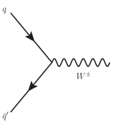
Figure 1: Leading order (a) $W$ and (b) $Z$ boson production via quark-antiquark annihilation. The production is dominated by $q=u,d$ valence quarks. The $\gamma^{*}$ contribution interferes with the $Z$ diagram but is not shown.

The heavy vector boson production cross section in a $p\overline{p}$ collision is given by

$$\sigma(V)=\int\sigma_{0,V}f(x_{q})\overline{f}(x_{\overline{q}})dx_{q}dx_{\overline{q}}$$

in which $\sigma_{0,V}$ is the cross section for production of a vector boson by a quark, antiquark pair with Feynman $x$ values of $x_{q}$ and $x_{\overline{q}}$ respectively, and $f(x_{q})$ and $\overline{f}(x_{\overline{q}})$ are the parton distribution functions for the proton and antiproton. As defined here, contributions from pure $\gamma*$ and $Z/\gamma*$ interference terms are not included but are accounted for in comparisons with theory in the measurements we describe.

The remainder of this section includes a summary of current $W$ and $Z$ cross section measurements that the Tevatron and their comparisons with theory. As previously mentioned, these measurements of $W$ and $Z$ boson production cross sections primarily a test QCD rather than electroweak theory. We include them here since detailed study of heavy gauge boson states are central to tests of electroweak theory and, therefore, it is important consider how well their production in $p\overline{p}$ collisions is understood.

The cross section times branching fraction of $W$ and $Z$ bosons is measured in the fully-leptonic decay channels $W\rightarrow\ell\nu$ and $Z\rightarrow\ell\ell$, where $\ell\equiv e,\mu,\tau$. While the final states involving $\tau$-leptons are important for many reasons, we restrict ourselves to the $e$ and $\mu$ final states for the cross section discussion since these give the highest precision measurements. The fully-leptonic decay channels are chosen over hadronic channels for these measurements, since the latter suffer from large backgrounds to due to the hadronic decay of jets produced by QCD processes.

III.1.1 $W$ and $Z$ Cross Sections

Using a next-to-next to leading order (NNLO) prediction [13] calculated with the MRST2004 NNLO parton distribution function [14] and the SM branching fractions for the $W$ and $Z$ bosons into fully-leptonic final states, the cross-section times branching fractions are calculated to be

$$\sigma(p\overline{p}\rightarrow W)\times B(W\to\ell\nu)=2687\pm 54\ \mathrm{pb}.$$

and

$$\sigma(p\overline{p}\rightarrow Z)\times B(Z\to\ell\ell)=251.9^{+5.0}_{-11.8}\ \mathrm{pb}.$$

The uncertainties are a combination of the MRST uncertainties and the difference between the central value above and that computed using the CTEQ6.1M parton distribution functions [15].

The $W$ and $Z$ cross sections times branching fractions to fully-leptonic final states have been measured by CDF [16] using $\int{\cal L}~{}dt=72$ pb^-1. The results for electron and muon channels combined are

$$\sigma(p\overline{p}\rightarrow W)\times B(W\to\ell\nu)=$$

$${}2749\pm 10\rm{(stat.)}\pm 53\rm{(syst.)}\pm 165\rm{(lumi.)}\ \mathrm{pb}$$

and

$$\sigma(p\overline{p}\rightarrow Z)\times B(Z\to\ell\ell)=$$

$${}254.9\pm 3.3\rm{(stat.)}\pm 4.6\rm{(syst.)}\pm 15.2\rm{(lumi.)}\ \mathrm{pb}.~{}~{}~{}~{}~{}~{}`$$

The measurements of the $Z$ cross section include additional contributions from $\gamma*$ and $Z/\gamma*$ interference which give events that are experimentally indistinguishable from the $Z$ process. The size of these contributions depends on the $Z/\gamma*$ mass range considered. For the range $60\ \mathrm{GeV/c}^{2}\leq M(Z/\gamma*)<130\ \mathrm{GeV/c}^{2}$ these contributions increase the cross section by a factor $1.019\pm 0.001$ relative to the $Z$-only cross section, and for the mass range $66\ \mathrm{GeV/c}^{2}\leq M(Z/\gamma*)<116\ \mathrm{GeV/c^{2}}$, the cross section is increased by a factor $1.004\pm 0.001$.

A precision measurement of the ratio $R$ of $W$ and $Z$ cross section times branching fraction given by

$$R=\frac{\sigma(p\overline{p}\rightarrow W)\times B(W\to\ell\nu)}{\sigma(p\overline{p}\rightarrow Z)\times B(Z\to\ell\ell)}$$

can be used to test the SM. For example, new high mass resonances decaying to either $W$ or $Z$ bosons could lead to a deviation of the measured value of $R$ from the SM expectation.

Important systematic uncertainties such as the integrated luminosity uncertainty cancel in the measurement of $R$. The ratio $R$ has been measured by CDF [16] using $\int{\cal L}~{}dt=72$ pb^-1 to be

$$R=10.84\pm 0.15{\rm(stat.)}\pm 0.14{\rm(syst.)}$$

This measurement has a precision of 1.9% and is consistent with SM expectation at NNLO of 10.69 $\pm$ 0.08 [13].

A summary of the results are shown in Tab. 1.

	Integrated	Data	Predicted
Channel	Luminosity	Yield	Background	$A\times\epsilon$	Measured $\sigma\times$ Br (pb)
$W\to e\nu$	72 pb-1	37584	$1762\pm 300$	$0.1795^{+0.0034}_{-0.0038}$	$2.771\pm 0.014^{+0.062}_{-0.056}\pm 0.166$ nb
$W\to\mu\nu$	72 pb-1	31722	$3469\pm 151$	$0.1442^{+0.0031}_{-0.0034}$	$2.722\pm 0.015^{+0.066}_{-0.061}\pm 0.163$ nb
$e\nu$ and $\mu\nu$	—	—	—	—	$2.749\pm 0.010\pm 0.053\pm 0.165$ nb
$Z\to ee$	72 pb-1	4242	$62\pm 18$	$0.2269^{+0.0047}_{-0.0048}$	$255.8\pm 3.9^{+5.5}_{-5.4}\pm 15.3$ pb
$Z\to\mu\mu$	72 pb-1	1785	$13\pm 13$	$0.0992^{+0.0028}_{-0.0031}$	$248.0\pm 5.9^{+8.0}_{-7.2}\pm 14.8$ pb
$ee$ and $\mu\mu$	—	—	—	—	$254.9\pm 3.3\pm 4.6\pm 15.2$ pb

Table 1: The measured integrated luminosity, yield, background, signal acceptance times efficiency and resulting $\sigma\times\mathrm{Br}$ for each of the four $Z$ cross section times branching ratio analyses by the CDF Collaboration in [16]. The combination of the dielectron and dimuon channels using the BLUE method is also shown. The $Z/\gamma*$ results have been corrected to $Z$ only as described in the text.

The individual results are in good agreement with each other and with the prediction from theory.

Even with the moderate sample sizes of these measurements, the $W$ and $Z$ cross section results are limited by the systematic uncertainty from the luminosity measurements. Because of this, further improvement in these measurements is not anticipated. CDF and D0 Collaborations continue to use $Z$-boson production to measure experimental efficiencies acceptances and cross-checks on temporal or instantaneous luminosity dependence of detector response. The updated cross section results could be reinterpreted as measurements of the integrated luminosity.

III.2 $W$ Boson Mass

At tree level, the $W$ boson mass is fully-determined by the electromagnetic fine structure constant, the weak Fermi coupling and the cosine of the weak mixing angle. When higher-order EW corrections, like those shown in Fig. 2, are included, the expression is modified to [17]

$$M_{W}^{2}=\frac{\hbar^{3}\pi\alpha_{EM}}{\sqrt{2}G_{F}}\frac{1}{(1-M_{W}^{2}/M_{Z}^{2})(1-\Delta r)}$$ (3)

in which $M_{W}$ (and later $\Gamma_{W}$) correspond to the parameters of a Breit-Wigner distribution with an $s$-dependent width. The term $\Delta r$ includes the effects of radiative corrections and depends on $M_{t}^{2}$ and $\log M_{H}$, where $M_{t}$ and $M_{H}$ are the top quark and Higgs boson masses, respectively. Measurement of the $W$ boson mass can be used to constrain the allowed Higgs boson mass. The precisions of the $W$ boson and top quark mass measurements are currently the limiting factors in the indirect constraint on the Higgs boson mass and are shown in Fig. 3. Earlier measurements of the $W$ boson mass have been made by the LEP experiments [18; 19; 20; 21] and CDF [22] and D0 [23] in Run I of the Tevatron.

Figure 2: Feynman diagrams showing corrections to the $W$ boson mass from (a) the top quark and (b) the SM Higgs boson.

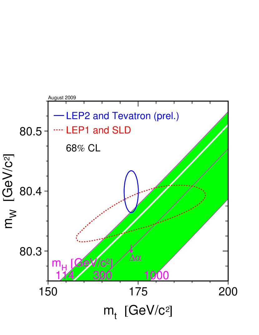
Figure 3: The measured top quark and $W$ boson masses and a band of allowed Higgs boson masses.[24] This includes the recent results summarized in the text.

Signal-to-background and resolution considerations dictate use of the $W\to e\nu$ and $W\to\mu\nu$ decays modes for the $W$ boson mass measurement at the Tevatron. The momentum component of the neutrino along the beam direction cannot be inferred in $p\overline{p}$ collision events, so the $W$ invariant mass cannot be reconstructed from its decay products and other variables are used to determine the mass. Three variables are used: (1) the lepton ($e$ or $\mu$) transverse momentum $p_{T}^{\ell}$, (2) the (inferred) neutrino transverse momentum $p_{T}^{\nu}$ and (3) the transverse mass, $m_{T}\equiv\sqrt{p_{T}^{\ell}p_{T}^{\nu}[1-\cos(\delta\phi)]}$ in which $\delta\phi$ is the lepton-neutrino opening angle in the plane transverse to the beam. Although these variables are highly correlated, their systematic uncertainties are dominated by different sources, so the results are combined taking their statistical and systematic correlations into account.

The event decay kinematics in the transverse plane are fully characterized by two quantities: (1) the lepton transverse momentum $\vec{p}_{T}^{\ell}$ and (2) the transverse momentum of the hadronic recoil $\vec{u}_{T}$ required to balance the transverse momentum of the the $W$. The hadronic recoil is defined as the vector sum of all energy measured in the calorimeter excluding that deposited by the lepton. From these two measurements, the neutrino transverse momentum is inferred: $-\vec{p}_{T}^{\nu}=\vec{p}_{T}^{\ell}+\vec{u_{T}}$. In practice, the recoil is computed using the event transverse missing energy ($E\kern-6.00006pt\raise 0.43057pt\hbox{/}_{T}$) measured in the calorimeter after removing the contribution to calorimeter energy associated with the lepton. The $W$ boson mass is determined by generating predicted distributions (templates) of the three measurement variables for a range of input $W$ boson mass hypotheses. These are generated using dedicated fast Monte Carlo simulation programs, and the mass is determined by performing a binned maximum likelihood fit of these templates to the distributions observed in data. The Run II measurements use a blinding technique in which an unknown offset is added to the value returned from the fits until the analyses are finished. At that point, the offset is removed to reveal the true value. The results from the different fit variables ($p_{T}^{\ell},\ p_{T}^{\nu},\ m_{T}$) and final states ($e$ or $\mu$) are combined using the BLUE algorithm [25; 26].

Both D0 and CDF have reported mass measurements using Run II data. The CDF result [1] uses $\int{\cal L}~{}dt=0.2$ fb^-1 and results are reported for $W\to e\nu$ and $W\to\mu\nu$ decays. The D0 result [27] uses $\int{\cal L}~{}dt=1.0$ fb^-1 and results are reported for the $W\to e\nu$ decay mode only. Candidate events are selected by requiring a single high-$p_{T}$ isolated charged lepton and large $E\kern-6.00006pt\raise 0.43057pt\hbox{/}_{T}$. Tab. 2 shows the kinematic selection requirements, event yields and background fraction for the $W$ event selections.

	CDF		D0
	000$W\to e\nu$000	000$W\to\mu\nu$000	000$W\to e\nu$000
$\int{\cal L}~{}dt$	0.2 fb-1	0.2 fb-1	1.0 fb-1
$E_{T}^{\ell}$, cal	$>30$ GeV	—	$>25$ GeV
$p_{T}^{\ell}$, trk	$>18\ {\rm GeV/c}$	$>30\ {\rm GeV/c}$	$>10\ {\rm GeV/c}$
$|\eta_{\ell}|$			$<1.05$
$E\kern-6.00006pt\raise 0.43057pt\hbox{/}_{T}$	$>30\ {\rm GeV/c}$	$>30\ {\rm GeV/c}$	$>25\ {\rm GeV/c}$
$u_{T}$	$<15\ {\rm GeV/c}$	$<15\ {\rm GeV/c}$	$<15\ {\rm GeV/c}$
Yield	63964	51128	499830
Background	7.5%	1.1%	4.0%

Table 2: The integrated luminosity, kinematic selection, event yield and backgrounds for the CDF and D0 $W$ boson mass analyses. The background is given as a percentage of the total yield.

The backgrounds include $Z\to\ell\ell$ events in which one lepton escapes identification, $WW$ diboson events, and misidentification backgrounds in which the lepton is either a jet misidentified as an electron or a muon from semileptonic decay of hadrons in which the rest of the associated hadronic jet is not reconstructed. An additional source of events are the sequential decays $W\to\tau\nu\to\ e\nu\nu\nu$ and $W\to\tau\nu\to\mu\nu\nu\nu$. The CDF analysis treats these as signal while the D0 analysis incorporates these into the background template distributions.

The in situ calibration of charged particle momenta (CDF) and calorimetric measurement of electron energy (CDF, D0) is of crucial importance to this result. The CDF analysis uses a calibration of the tracker momentum scale ($p$) determined from dimuon and dielectron decays of $J/\psi$, $\Upsilon$ and $Z$ particles. This calibration is then transferred to the calorimeter energy measurement ($E$) using the $E/p$ ratio. A final improvement is made for the $W\to e\nu$ mode by incorporating an additional calorimeter calibration based on $Z\to ee$ decays. The D0 analysis uses calorimeter energy measurements, and the calibration is based on the mass reconstructed in $Z\to ee$ events and a detailed simulation of the calorimeter response. For both experiments, this calibration is the dominant source of systematic uncertainty. Other sources of systematic uncertainty arise from trigger efficiency, lepton identification efficiency, correlation (in)efficiency such as occurs when the hadronic recoil is near the charged lepton, backgrounds, electroweak and strong contributions to the production and decay model and the parton distribution functions.

The $m_{T}$ distributions for each channel are shown in Fig. 4, and the results from each channel and the combinations of the channels for each experiment are shown in Tab. 3. The systematic uncertainties are dominated by the lepton energy calibration. This contributes 17 MeV uncertainty to the CDF $p_{T}^{\ell}$ and $p_{T}^{\nu}$ channels, 30 MeV to the CDF $m_{T}$ channel and 34 MeV to each D0 channel.

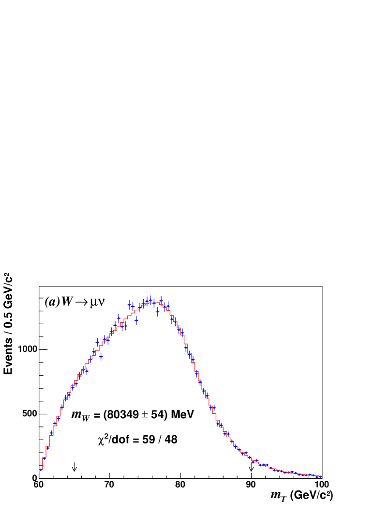
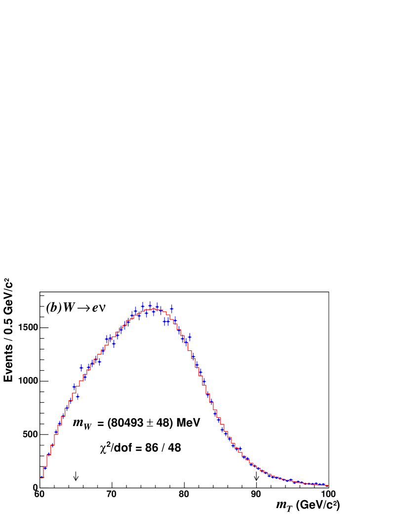
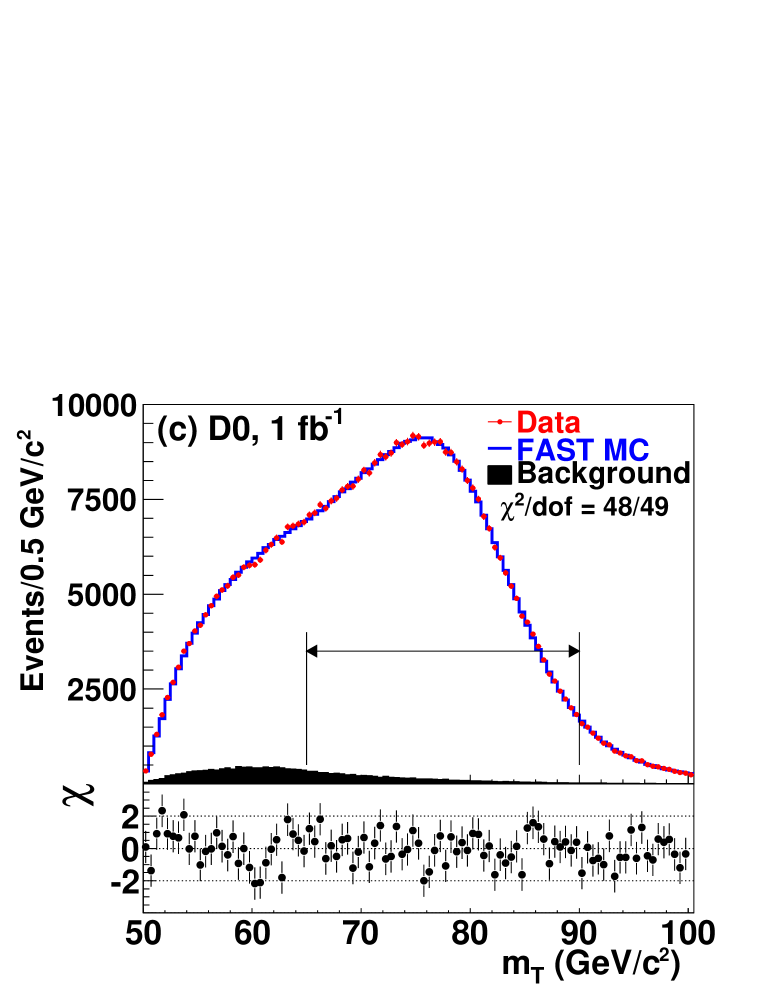
Figure 4: The $m_{T}$ distributions for (a) the CDF $W\to\mu\nu$ channel, (b) the CDF $W\to e\nu$ channel and (c) the D0 $W\to e\nu$ channel.

		000$M_{W}$ (MeV)000	$\chi^{2}/$dof
CDF $W\to e\nu$	$m_{T}$	$80493\pm 48\pm 39$	86/48
	$p_{T}^{e}$	$80451\pm 58\pm 45$	63/62
	$E\kern-6.00006pt\raise 0.43057pt\hbox{/}_{T}$	$80473\pm 57\pm 54$	63/62
Combined		$80477\pm 62$
CDF $W\to\mu\nu$	$m_{T}$	$80349\pm 54\pm 27$	59/48
	$p_{T}^{\mu}$	$80321\pm 66\pm 40$	72/62
	$E\kern-6.00006pt\raise 0.43057pt\hbox{/}_{T}$	$80396\pm 66\pm 46$	44/63
Combined		$80352\pm 60$
CDF $W\to e\nu+\mu\nu$		$80413\pm 34\pm 34$
D0 $W\to e\nu$	$m_{T}$	$80401\pm 23\pm 37$	48/49
	$p_{T}^{e}$	$80400\pm 27\pm 40$	39/31
	$E\kern-6.00006pt\raise 0.43057pt\hbox{/}_{T}$	$80402\pm 23\pm 43$	32/31
D0 Combined		$80401\pm 21\pm 38$

Table 3: The individual CDF and D0 $W$ boson mass results and their combinations. When two uncertainties are given, the first is the statistical uncertainty and the second is the systematic uncertainty.

These results are shown along with previous measurements in Fig. 5. The world average

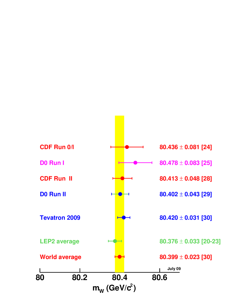
Figure 5: Ideogram of previous measurements, the Run II CDF and D0 measurements and the new world average. The Ref. is shown to the right of each measurement as [XX].

combination [28; 24] has been updated with these measurements using the BLUE [25; 26] algorithm including correlations. The result is

$$M_{W}=80.420\pm 0.031\ \mathrm{GeV/c}^{2}.$$

Because the systematic uncertainties are dominated by the statistical precision of the calibrations determined from control data samples, the systematic uncertainty in future measurements is expected to improve as the integrated luminosity increases. The ultimate limiting systematic is expected to be that introduced by the parton distribution functions. In the current results, this contributes an uncertainty of 11 MeV to all channels with a 100% correlation among the channels.

III.3 $W$ Width

Like the $W$ boson mass, the width $\Gamma_{W}$ is also predicted by the SM. It is given by

$$\Gamma_{W}=[3+2N_{C}(1+\frac{\alpha_{S}}{\pi})]\frac{G_{F}M_{W}^{3}}{6\sqrt{2}\pi}(1+\delta)$$ (4)

in which $N_{C}=3$ is the number of colors, $1+\alpha_{S}/\pi$ is the QCD correction factor to first order, and $\delta=2.1$% [29] is an EW correction factor. Direct measurements of $\Gamma_{W}$ were made by CDF [30] and D0 [31] using Tevatron Run I data and combined [31]. Measurements were also made by the experiments at LEP [18; 19; 20; 21].

Because the $W$ boson mass is distributed according to a Breit-Wigner, there is a tail at large mass values. The $W$ boson width result is obtained using the $m_{T}$ distribution in a region where the shape and event yield are dominated by events from the high mass region of the Breit-Wigner with limited impact from detector resolution effects. As for the $W$ boson mass measurement, a binned likelihood comparison of the observed spectrum to templates generated for different $W$ boson widths is used to extract the numerical value.

The $W$ width was measured by CDF [32] and D0 [33] using Run II data. The CDF result uses a data set of $\int{\cal L}~{}dt=0.35$ fb^-1 and the electron and muon final states. The D0 result uses $\int{\cal L}~{}dt=1$ fb^-1 and the electron final state. The D0 data set is the same one used for the $W$ boson mass measurement. Similar dedicated simulations and processing were used for the $W$ width measurement as were used for the $W$ boson mass measurement. D0 used a different hadronic recoil procedure [34]. The new procedure gives a $W$ boson mass result consistent with the standard method. Fig. 6 shows the high mass region of the $m_{T}$ distribution for the three channels analyzed: the CDF $W\to\mu\nu$ channel, the CDF $W\to e\nu$ channel and the D0 $W\to e\nu$ channel.

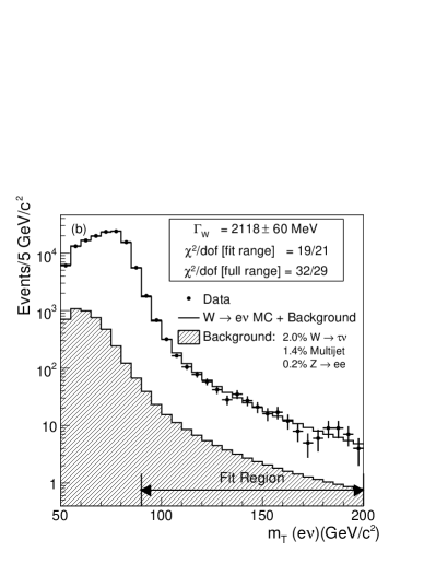
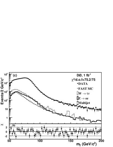
Figure 6: The $m_{T}$ distributions used for the $\Gamma_{W}$ measurement. (a) The CDF $W\to\mu\nu$ channel. (b) The CDF $W\to e\nu$ channel. (c) The D0 $W\to e\nu$ channel.

The $\Gamma_{W}$ results are given in Tab. 4 and shown in Fig. 7. The systematic uncertainties are dominated by hadronic recoil scale and resolution uncertainties. These contribute 54(49) MeV for the CDF $W\to e\nu\ (W\to\mu\nu)$ channel and 41 MeV to the D0 result. Other important sources include the lepton scale uncertainty and background uncertainty which are one half to two thirds the size of the hadronic recoil uncertainty.

Channel	Yield	Fit Range(${\rm GeV/c}^{2}$)	$\Gamma_{W}$ (MeV)	$\chi^{2}/$ndof
CDF $W\to\mu\nu$	2619	$90<m_{T}<200$	$1948\pm 67\pm 71$	17/21
CDF $W\to e\nu$	3436	$90<m_{T}<200$	$2118\pm 60\pm 79$	19/21
CDF Combined			$2032\pm 45\pm 57$
D0 $W\to e\nu$	5272	$100<m_{T}<200$	$2028\pm 39\pm 61$	75.2/75

Table 4: The $\Gamma_{W}$ measurements. For the result, the first uncertainty is the statistical uncertainty and the second is the systematic uncertainty.

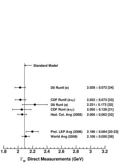
Figure 7: Summary of the $\Gamma_{W}$ measurements. The Hadron Collider Average and World Average results do not include the D0 [33] result.

III.4 Forward-backward Asymmetry, $A_{FB}$

Production of $Z$ bosons at the Tevatron is dominated by the process $q\overline{q}\to Z/\gamma^{*}$ in which $q=u,d$ are proton valence quarks. The SM couplings of the $Z$ and $\gamma$ to quarks depend on the quark charge $Q$, the isospin $I_{3}$, and the sine of the weak mixing angle $\sin^{2}\theta_{W}$. The differential cross section as a function of the direction of the fermion resulting from the $Z/\gamma^{*}$ decay is given by

$$\frac{d\sigma}{d\cos\theta}=a(1+\cos^{2}\theta)+b\cos\theta$$ (5)

in which $\theta$ is the angle of the fermion from the $Z/\gamma^{*}$ decay measured relative to the incoming quark direction in the $Z/\gamma^{*}$ rest frame. The relative $Z$ and $\gamma^{*}$ contributions to the cross section vary as a function of the $Z/\gamma^{*}$ mass, and differences in the $Z$ and $\gamma$ couplings to quarks result in different angular distributions for the decay products for up-type ($I_{3}=+1/2$) and down-type ($I_{3}=-1/2$) quarks. Together, these two effects produce mass and flavor dependence in the coefficients $a$ and $b$ which can be calculated assuming the SM.

The forward-backward $Z/\gamma^{*}$ production charge asymmetry is defined as

$$A\equiv\frac{\sigma_{+}-\sigma_{-}}{\sigma_{+}+\sigma_{-}}$$

in which $\sigma_{+}$ and $\sigma_{-}$ are the integrated cross sections for the cases $\cos\theta>0$ and $\cos\theta<0$ respectively. The asymmetry extracted experimentally is given by

$$A_{FB}=\frac{N_{+}-N_{-}}{N_{+}+N_{-}}$$ (6)

in which $N_{+}$ and $N_{-}$ are the acceptance, efficiency and background corrected fermion yields in the forward $(\cos\theta>0$) and backward $(\cos\theta<0)$ directions respectively. Measuring the asymmetry rather than differential cross sections allows cancellation of many systematic uncertainties, particularly those affecting the overall normalization.

Measurements of the asymmetry as a function of dielectron mass have been made by both CDF [35] and D0 [36] using the dielectron final state. The CDF result uses a sample with $\int{\cal L}~{}dt=72$ pb^-1, and the D0 measurement uses $\int{\cal L}~{}dt=1.1$ fb^-1. The selection criteria are similar to those for the $Z$ cross section measurements although a larger dielectron mass range was selected for the asymmetry measurements. Two experimental issues of particular importance to these measurements are (1) controlling asymmetries in either detector acceptance or selection efficiency as a function of dielectron mass and (2) limiting the impact of electron charge misidentification.

In Tab. 5, the dielectron mass range and the predicted and measured values of $A_{FB}$ for each mass bin from the D0 measurements are shown, and Figs. 8 and 9 show the measured asymmetries and the SM predictions as a function of mass for the CDF and D0 results respectively.

Dielectron Mass	$A_{FB}$
Range (GeV/c)2	Pythia	ZGrad	Measured
$50-60$	$-0.293$	$-0.307$	$-0.262\pm 0.066\pm 0.072$
$60-70$	$-0.426$	$-0.431$	$-0.434\pm 0.039\pm 0.040$
$70-75$	$-0.449$	$-0.452$	$-0.386\pm 0.032\pm 0.031$
$75-81$	$-0.354$	$-0.354$	$-0.342\pm 0.022\pm 0.022$
$81-86.5$	$-0.174$	$-0.166$	$-0.176\pm 0.012\pm 0.014$
$86.5-89.5$	$-0.033$	$-0.031$	$-0.034\pm 0.007\pm 0.008$
$89.5-92$	$~{}~{}0.051$	$~{}~{}0.052$	$~{}~{}0.048\pm 0.006\pm 0.005$
$92-97$	$~{}~{}0.127$	$~{}~{}0.129$	$~{}~{}0.122\pm 0.006\pm 0.007$
$97-105$	$~{}~{}0.289$	$~{}~{}0.296$	$~{}~{}0.301\pm 0.013\pm 0.015$
$105-115$	$~{}~{}0.427$	$~{}~{}0.429$	$~{}~{}0.416\pm 0.030\pm 0.022$
$115-130$	$~{}~{}0.526$	$~{}~{}0.530$	$~{}~{}0.543\pm 0.039\pm 0.028$
$130-180$	$~{}~{}0.593$	$~{}~{}0.603$	$~{}~{}0.617\pm 0.046\pm 0.013$
$180-250$	$~{}~{}0.613$	$~{}~{}0.600$	$~{}~{}0.594\pm 0.085\pm 0.016$
$250-500$	$~{}~{}0.616$	$~{}~{}0.615$	$~{}~{}0.320\pm 0.150\pm 0.018$

Table 5: The expected and measured asymmetries as a function of dielectron mass (D0). For the measured values, the first uncertainty is statistical and the second is systematic.

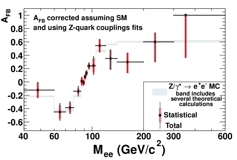
Figure 8: Dielectron forward-backward asymmetry as a function of dielectron mass(CDF).

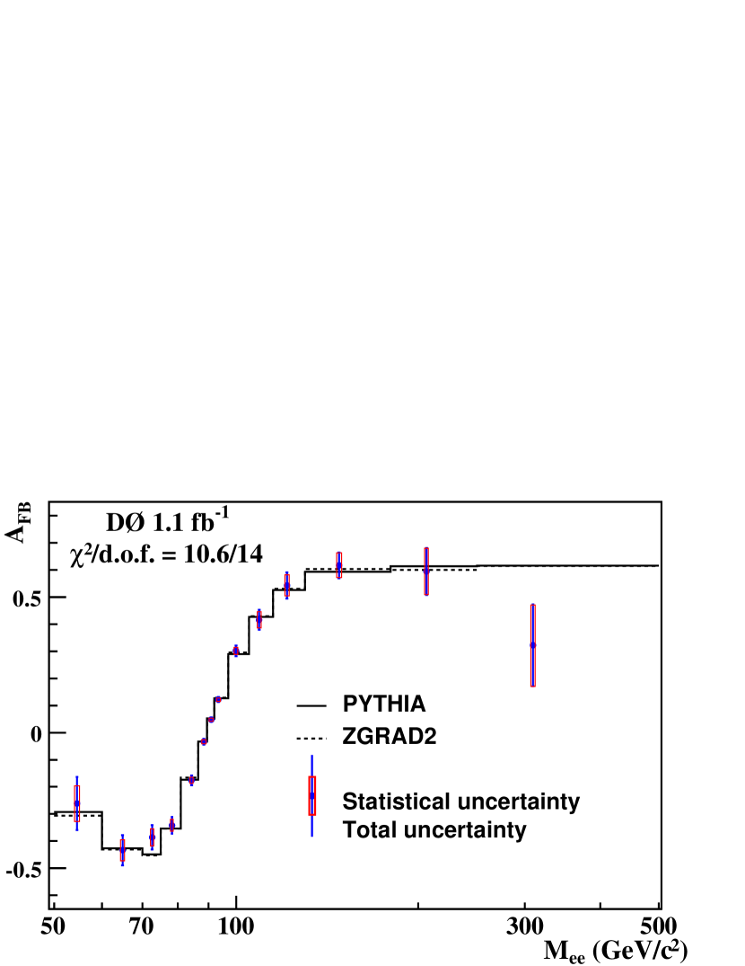
Figure 9: Dielectron forward-backward asymmetry as a function of dielectron mass (D0).

Using these measurements and the SM prediction for the coefficients $a$ and $b$, $\sin^{2}\theta_{W}^{eff}$ can be determined. Here $\theta_{W}^{eff}$ is the weak mixing angle including higher order corrections. The current world average is

$$\sin^{2}\theta_{W}^{eff}=0.23149\pm 0.00013$$

using the $\overline{MS}$ scheme [37]. Among the measurements used for the world average are two, the charge asymmetry for $b$-quark production [11] from LEP and SLD and the measurement from NuTeV [38], which differ from the world average by more than two standard deviations.

The values for $\sin^{2}\theta_{W}^{eff}$ extracted using fits to the CDF and D0 $A_{FB}$ distributions are

$$\sin^{2}\theta_{W}^{eff}=0.2238\pm 0.0040\ \mathrm{(stat)}\pm 0.0030\ \mathrm{(syst)}$$

for CDF and

$$\sin^{2}\theta_{W}^{eff}=0.2327\pm 0.0018\ \mathrm{(stat)}\pm 0.0006\ \mathrm{(syst)}$$

for D0. Fig. 10 shows these results compared to other measurements. The results from D0 are comparable in precision to other measurements for light quarks. The current Tevatron results are limited by sample statistics, but by the end of the Tevatron running, CDF and D0 are expected to have the most precise measurements of $\sin^{2}\theta_{W}^{eff}$ for light quarks.

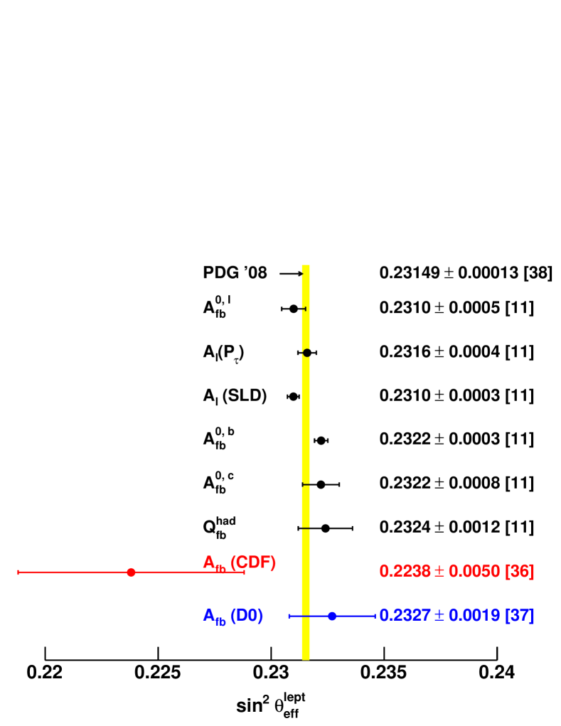
Figure 10: Comparison of the Tevatron asymmetry results with those from other experiments.

CDF also removed the assumption of SM quark couplings and determined values from a four parameter fit of $A_{FB}$ measurements to the SM prediction as function of the vector and axial vector couplings for $u$ and $d$ quarks. The fit has a $\chi^{2}/\mathrm{dof}=10.4/11$, and the resulting coupling values are shown (with the SM values) in Fig. 11. No evidence of deviation from the SM is observed.

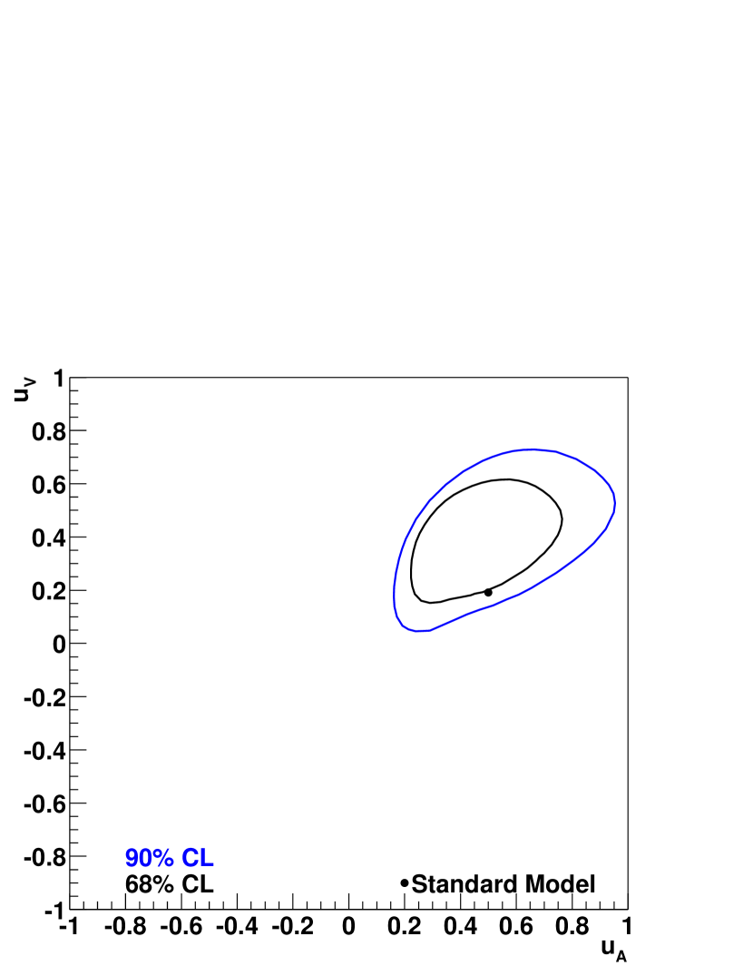
Figure 11: The $Zuu$ and $Zdd$ coupling constants. [35]

III.5 Dibosons

III.5.1 Trilinear Gauge Couplings (TGCs)

The non-Abelian nature of the gauge theory describing the electroweak interactions leads to a striking feature of the theory. In quantum electrodynamics, the photons carry no electric charge and thus lack photon-to-photon couplings and do not self-interact. In contrast, the weak vector bosons carry weak charge and do interact amongst themselves through trilinear and quartic gauge boson vertices. Fig. 12 shows the tree-level diagram for diboson production involving trilinear gauge couplings.

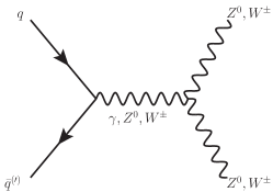
Figure 12: Leading order diagram for diboson production via quark-antiquark annihilation involving the trilinear gauge coupling.

The SM Lagrangian that describes the $WWV(V=Z,\gamma)$ interaction is given by

$${\cal L}^{\rm SM}_{WWV} = ig_{WWV}[(W^{+}_{\mu\nu}W^{-\mu}-W^{+\mu}W^{-}_{\mu\nu})V^{\nu}$$

$${}+W^{+}_{\mu}W^{-}_{\nu}V^{\mu\nu}]$$

where $W^{\mu}$ denotes the $W$ field, $W_{\mu\nu}=\partial_{\mu}W_{\nu}-\partial_{\nu}W_{\mu}$, $V_{\mu\nu}=\partial_{\mu}V_{\nu}-\partial_{\nu}V_{\mu}$, the overall couplings are $g_{WW\gamma}=-e$ and $g_{WWZ}=-e\cot\theta_{W}$, and $\theta_{W}$ is the weak mixing angle [39]. At tree level in the SM, the trilinear boson couplings involving only neutral gauge bosons ($\gamma$ and $Z$) vanish because neither the photon nor the $Z$ boson carry electric charge or weak hypercharge.

A common approach used to parameterize the low energy effects from high-scale new physics is the effective Lagrangian approach that involves additional terms not present in the SM Lagrangian [39]. This approach is convenient because it allows for diboson production properties measured in experiments to be interpreted as model-independent constraints on anomalous coupling parameters which can be compared with the predictions of new physics models.

A general form for the $WWV$ Lorentz-invariant interaction Lagrangian with anomalous coupling parameters $g_{1}^{V}$, $\kappa_{V}$, and $\lambda_{V}$ is given by [39; 40]

$${\cal L}^{\rm eff}_{WWV} = ig_{WWV}[g_{1}^{V}(W^{+}_{\mu\nu}W^{-\mu}-W^{+\mu}W^{-}_{\mu\nu})V^{\nu}$$

$${}+~{}\kappa_{V}W^{+}_{\mu}W^{-}_{\nu}V^{\mu\nu}$$

$${}+~{}\frac{\lambda_{V}}{M_{W}^{2}}W^{+\nu}_{\mu}W^{-\rho}_{\nu}V^{\mu}_{\rho}]$$

Note that ${\cal L}^{\rm eff}$ reduces to ${\cal L}^{\rm SM}$ for the values $\lambda_{\gamma}=\lambda_{Z}=0$ and $g_{1}^{\gamma}=g_{1}^{Z}=\kappa_{\gamma}=\kappa_{Z}=1$. Deviations from the SM values of the coupling parameters are denoted by $\Delta g_{1}^{V}$, $\Delta\kappa_{V}$, and $\Delta\lambda_{V}$. We have assumed that $C$ and $P$ are conserved in the interaction Lagrangian. There is no reason to believe that this assumption is valid unless the physics that leads to anomalous couplings respects these symmetries. It is straightforward to include additional terms that violate $C$ and $P$, but we refrain from doing so in order to keep the discussion simple.

Electromagnetic gauge invariance requires $\Delta g_{1}^{\gamma}=0$. The $W$ boson magnetic moment $\mu_{W}$ and the electric quadrupole moment $Q_{W}$ are related to the coupling parameters by

$$\mu_{W}=\frac{e}{2m_{W}}(1+\kappa_{\gamma}+\lambda_{\gamma})$$

and

$$Q_{W}=-\frac{e}{m^{2}_{W}}(\kappa_{\gamma}-\lambda_{\gamma})$$

The anomalous couplings (aside from $g_{1}^{\gamma}$) are usually assumed to have some dependence on an energy scale (form factors) which suppresses them at large scales to avoid violation of tree-level unitarity in the diboson production amplitude [41; 42]. The parameterization generally used for the energy dependence of a given coupling parameter $\alpha$ is

$$\alpha(\hat{s})=\frac{\alpha_{0}}{(1+\hat{s}/\Lambda^{2})^{2}}$$

where $\sqrt{\hat{s}}$ is the partonic center-of-mass collision energy, $\alpha_{0}$ is the value of the coupling parameter in the limit $\hat{s}\rightarrow 0$, and $\Lambda$ is the cutoff scale.

The $\sqrt{\hat{s}}$ distribution used in the measurements described in this Section is obtained through Monte Carlo simulation of the collision physics. With the substantially increased diboson statistics that will be available at the LHC, anomalous TGC searches can be reported as a function of $\sqrt{\hat{s}}$ in diboson decay channels resuting in fewer than two neutrinos, where the $\sqrt{\hat{s}}$ can be estimated on an event-by-event basis. This approach would lead to improved sensitivity and less dependence on ad-hoc form factors as compared to the standard approach.

When reporting coupling limits from hadron collider data, the value of $\Lambda$ is taken to be close to the hadron collision energy; even large variations (e.g. 50%) of $\Lambda$ around this scale have minimal impact on the results. Physically, the scale $\Lambda$ can be considered the scale at which the new physics responsible for the anomalous coupling is directly accessible (e.g. through pair production of new particles). This approach is different from the effective field theory approach discussed in Section II, where the coefficients of higher-dimension operators are constants. While in the same spirit as effective field theory, the effective Lagrangian approach to anomalous couplings is different in practice. In particular, the form factors invoked in the effective Lagrangian approach are unnecessary in an effective field theory approach.

In the presence of new physics, neutral TGCs (those involving only $\gamma$ and $Z$ bosons) can contribute to $Z\gamma$ and $ZZ$ production. As previously described, neutral TGCs are anomalous by their very nature since these couplings are absent in the SM. For each of the diboson final states $Z\gamma$ and $ZZ$, one can follow an analogous procedure to the anomalous charged TGCs (those involing a $W$ boson) by writing down the most general effective Lagrangian that respects Lorentz invariance and electromagnetic gauge invariance [43; 44]. Using prescriptions detailed in [43] and [44], the effective Lagrangians introduce anomalous coupling parameters $h_{i0}^{V}(V=\gamma,Z~{}{\rm and}~{}i=3,4)$ and $f_{j0}^{V}(V=\gamma,Z~{}{\rm and}~{}j=4,5)$ respectively, which can be constrained through an analysis of $Z\gamma$ and $ZZ$ production in high-energy collider data. It is important to note that, under the assumption of on-shell $Z$ bosons, the $Z\gamma Z$ couplings contributing to $Z\gamma$ production and $ZZ\gamma$ couplings contributing to $ZZ$ production are completely independent [44].

In general, the effect on observables from turning on anomalous TGCs are correlated. When we refer to “1D limits,” we refer to the limits derived on one parameter when the others are set to their SM values.

There are a few important differences regarding the study of diboson physics in particle collisions at LEP, Tevatron, and the LHC that are worth pointing out at this stage:

• At LEP, $e^{+}e^{-}$ collisions occur at a well-defined energy that is set by the accelerator. Therefore, the center-of-mass energy is known with good precision and there are no form factors in anomalous coupling analyses.

• In $e^{+}e^{-}$ collisions, the initial state has zero electric charge. Therefore, exclusive states with net charge, such as $WZ$ and $W\gamma$, cannot be produced at LEP. The $WW$ and $ZZ$ states can and have been produced and studied at LEP. A measurement of the $WW$ cross section over a scan in beam energy dramatically illustrates the existence of the $WWZ$ coupling in electroweak theory [45].

• At hadron colliders, $\sqrt{s}$ is fixed for long periods of time (defining different periods of the accelerator operation that change very infrequently) but $\sqrt{\hat{s}}$ varies collision by collision. Any anomalous couplings are likely to be $\sqrt{\hat{s}}$ dependent. The form factor ansatz used to cut off the anomalous coupling parameters at large $\sqrt{\hat{s}}$ to preserve S-matrix unitary of the amplitude reflects this dependence. For this reason, it is reasonable to expect that, once a sufficient amount of integrated luminosity has been acquired, the higher-energy reach afforded by high-energy hadron collisions will lead to better sensitivity to anomalous couplings as compared to the limits from LEP, despite larger backgrounds in a typical hadron collision event. In other words, hadron collisions at the Tevatron and LHC sample events with a larger average $\sqrt{\hat{s}}$ as compared to LEP collision energies and it is exactly those high $\sqrt{\hat{s}}$ events that are most sensitive to effects of anomalous couplings from new physics at higher energy scale.

• Because the Tevatron is a $p\bar{p}$ collider, the production cross sections for $W^{+}Z$ and $W^{-}Z$ are equal. The same is true for $W^{+}\gamma$ and $W^{-}\gamma$ production. When produced in a $pp$ collider such as the LHC, positive and negative net charge diboson states have different production cross sections (e.g. $\sigma(pp\rightarrow W^{+}Z)>\sigma(pp\rightarrow W^{-}Z)$).

III.5.2 $W\gamma$

The $W\gamma$ final state observed at hadron colliders provides a direct test of the $WW\gamma$ TGC. Anomalous $WW\gamma$ couplings lead to an enhancement in the production cross section and an excess of large $E_{T}$ photons. Both CDF and D0 have published measurements of the $W\gamma$ cross section using leptonic decays of the $W$ bosons and $\int{\cal L}~{}dt=0.2~{}\rm{fb}^{-1}$ [46; 47]. The signature of the $W\gamma$ signal is an isolated high $E_{T}$ lepton, an isolated high $E_{T}$ photon, and large $E\kern-6.00006pt\raise 0.43057pt\hbox{/}_{T}$ due to the neutrino from the $W$ decay. The dominant background is from $W$+jets where a jet mimics an isolated photon. A lepton-photon separation requirement in $\eta-\phi$ space of $\Delta R=\sqrt{(\Delta\eta)^{2}+(\Delta\phi)^{2}}>0.7$ is made by both CDF and D0 to suppress events with final-state radiation of the photon from the outgoing lepton and to avoid collinear singularities in theoretical calculations. A kinematic requirement on photon $E_{T}$ of $E_{T}>7(8)$ GeV is made by CDF (D0 ) in the analysis.

CDF measures

$$\sigma(p\bar{p}\rightarrow W\gamma+X)\times BR(W\rightarrow l\nu)$$

$${}=18.1~{}\pm~{}1.6\rm{(stat.)}~{}\pm~{}2.4\rm{(syst.)}~{}\pm~{}1.2\rm{(lum.)}~{}\rm{pb}$$

[46] in agreement with the next-to-leading order (NLO) theoretical expectation ($E_{T}>7$ GeV) [43] of $19.3~{}\pm~{}1.4$ pb. D0 measures

$$\sigma(p\bar{p}\rightarrow W\gamma+X)\times BR(W\rightarrow l\nu)$$

$${}=14.8~{}\pm~{}1.6\rm{(stat.)}~{}\pm~{}1.0\rm{(syst.)}\pm 1.0\rm{(lum.)}~{}\rm{pb}$$

[47] also in agreement with the NLO expectation ($E_{T}>8$ GeV) [43] of $16.0~{}\pm~{}0.4$ pb. Tab. 6 summarizes the $W\gamma$ cross section measurement results.

	D0 Analysis				CDF Analysis
	$e\nu\gamma$		$\mu\nu\gamma$		$e\nu\gamma$		$\mu\nu\gamma$
$\int{\cal L}\ dt$ (fb-1)	0.16		0.13		0.20 (0.17)		0.19 (0.18)
$W+$ jet(s)	59$\,\pm\,$	5	62$\,\pm\,$	5	60$\,\pm\,$	18	28$\,\pm\,$	8
$\ell eX$	1.7$\,\pm\,$	0.5	0.7$\,\pm\,$	0.2	$-$		$-$
$W\gamma\rightarrow\tau\nu\gamma$	0.42$\,\pm\,$	0.02	1.9$\,\pm\,$	0.2	1.5$\,\pm\,$	0.2	2.3$\,\pm\,$	0.2
$Z\gamma\rightarrow\ell\ell\gamma$	$-$		6.9$\,\pm\,$	0.7	6.3$\,\pm\,$	0.3	17.4$\,\pm\,$	1.0
Total Bkg.	61$\,\pm\,$	5	71$\,\pm\,$	5	67$\,\pm\,$	18	47$\,\pm\,$	8
$N_{\rm observed}$	112		161		195		128
$\sigma\times$ BR (pb)	13.9$\,\pm\,$	3.4	15.2$\,\pm\,$	2.5	19.4$\,\pm\,$	3.6	16.3$\,\pm\,$	2.9
Theory $\sigma\times$ BR	$16.0\pm 0.4$				$19.3\pm 1.4$

Table 6: Summary of the $W\gamma\rightarrow\ell\nu\gamma$ CDF [46] and D0 [47] cross section analyses compared with the theory [43]. For the CDF analysis, the luminosities with and without parentheses correspond to central and forward leptons, respectively. The theory cross section is the NLO calculation (in pb) from [43].

Both of the CDF and D0 $W\gamma$ cross section measurement are consistent with the SM expectations at NLO. In a more recent analysis [48], D0 uses four times more integrated luminosity as compared to [47] and adds photons reconstructed in their endcap calorimeters ($1.5<|\eta_{det}|<2.5$) to search for anomalous $WW\gamma$ couplings based on the observed photon $E_{T}$ spectrum [48] for photons with $E_{T}>9$ GeV. Additionally, the three-body transverse mass of the photon, lepton and $E\kern-6.00006pt\raise 0.43057pt\hbox{/}_{T}$ must exceed 120 ${\rm GeV/c}$ (110 ${\rm GeV/c}$) for the electron (muon) channel in order to suppress final state radiation. The photon $E_{T}$ spectrum and anomalous TGC limits are shown in Fig. 13. A LO simulation [49] of the $W\gamma$ signal is used with NLO corrections [50] applied to the photon $E_{T}$ spectrum. The one-dimensional limits at 95% confidence level (CL) are $-0.51<\Delta\kappa_{\gamma}<0.51$ and $-0.12<\lambda_{\gamma}<0.13$ for $\Lambda=2.0$ TeV.

Figure 13: The (a) photon $E_{T}$ distribution for the D0 $W\gamma$ analysis [48]. The photon $E_{T}$ distribution of events are used to constrain anomalous coupling parameters shown in (b).

The SM $W\gamma$ production involves interference between the amplitudes for a photon radiated off of an incoming quark (QED initial state radiation) and the photon produced from the $WW\gamma$ vertex. This interference leads to a zero amplitude for the SM in the photon angular distribution [51; 52; 53; 54]. In $W\gamma$ production, the radiation amplitude zero (RAZ) manifests itself as a dip at $\sim-1/3$ in the charged-signed rapidity difference $Q_{\ell}\times\Delta y$ between the observed photon and the charged lepton from decay of the $W$ boson [55]. Experimentally, the pseudorapidity difference $\Delta\eta$ is used in place of the rapidity difference $\Delta y$, since it involves only the production angle $\theta$ with respect to the beam line ($\eta=-\ln(\tan(\theta/2))$) and is a very good approximation to $\Delta y$ in the limit of massless particles. Using the same data they used to limits on $WW\gamma$ anomalous TGCs, D0 made a first detailed study of the $Q_{\ell}\times\Delta y$ to search for the RAZ effect [48].

Fig. 14(a) shows the $Q_{\ell}\times\Delta y$ distribution of data compared with the SM expectation, which has a 15% $\chi^{2}$ probability for compatibility between the data and the SM expectation, demonstrating a reasonable level of agreement. To specifically investigate the dip region around $Q_{\ell}\times\Delta y=-1/3$ indicative of the RAZ effect, a simple test statistic $R$ is constructed which is the ratio of the number events observed in a bin including the dip region to the number of events observed in a bin with more negative $Q_{\ell}\times\Delta y$ where a maximum is expected, based on Monte Carlo, from the SM including the total D0 acceptance in this analysis. A value of $R=0.64$ is observed in the data and it is determined that 28% of SM pseudo-experiments give a value as large or larger than 0.64.

A particular anomalous coupling hypothesis corresponding to $\kappa_{\gamma}=0$, $\lambda_{\gamma}=-1$ is chosen to test against as a null hypothesis since it is a specific model which leads to a $Q_{\ell}\times\Delta y$ distribution without a dip as shown in the inset of Fig. 14(b). Only the shape is tested such that the null “no-dip” distribution is normalized to the yield expected from the SM. The $R$ distribution for the SM and no-dip hypotheses are shown in Fig. 14(b) along with the value (0.64) observed in the data. From this analysis, the no-dip hypothesis is excluded at 2.6$\sigma$ Gaussian significance.

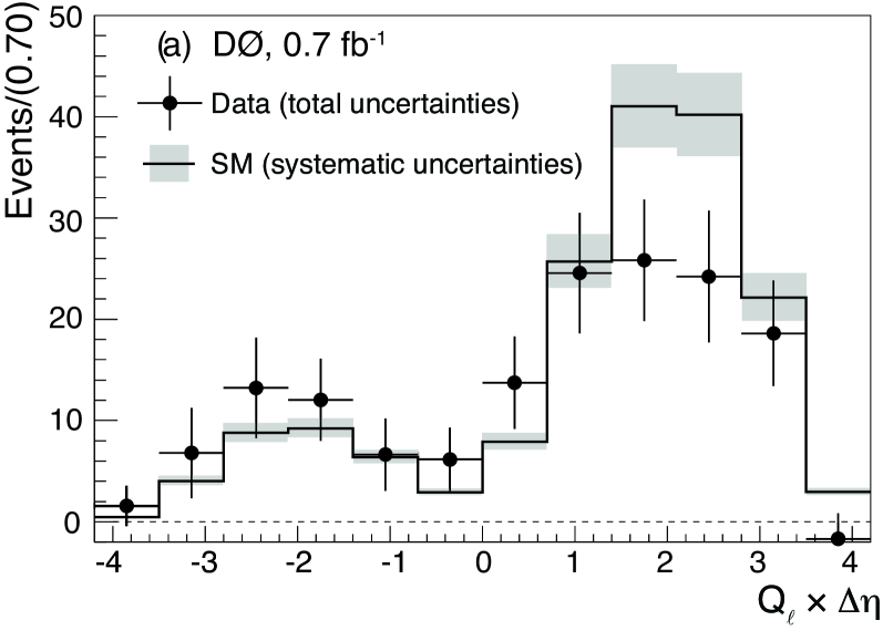
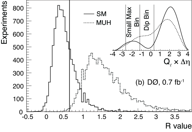
Figure 14: (a) The background-subtracted charge-signed rapidity difference of events is shown in along with the SM expectation from [48]. Consideration of the full covariance matrix gives a 15% $\chi^{2}$ probability for compatibility between the data and the SM expectation. (b) Distributions of the R-test statistic for the SM (solid line) and “no-dip” (dashed line) hypothesis pseudo-experiments from [48]. The data result is 0.64 shown by the vertical line where only 45 out of 10⁴ no-dip pseudo-experiment had a value smaller as small or smaller than 0.64. The R-test statistic is defined as the ratio of events in the “Dip Bin” to the “Small Max Bin”, as shown in the inset where the solid line is the SM expectation and the dashed line is for the no-dip hypothesis.

III.5.3 $Z\gamma$

As mentioned in Section III.5.1, photons do not directly couple to $Z$ bosons at tree-level in the SM. Therefore, observation of such a coupling would constitute evidence for new phenomena. The $Z\gamma$ final state at hadron colliders involves a combination of $ZZ\gamma$ and $Z\gamma\gamma$ couplings. Both CDF and D0 have made measurements of the $Z\gamma$ cross section in leptonic decay channels of the $Z$ boson. The signature of the $Z\gamma$ signal is two isolated high $E_{T}$ charged leptons having the same flavor and opposite charge with invariant mass consistent with decay of a $Z$ boson, and an isolated high $E_{T}$ photon. The dominant background is from $Z$+jets where a jet mimics an isolated photon. As in the $W\gamma$ analyses described in Section III.5.2, a lepton-photon separation requirement is imposed. A requirement of $\Delta R>0.7$ is made by both CDF and D0. Kinematic requirements on the photon $E_{T}$ of $E_{T}>7(8){\rm GeV/c}^{2}$ and the dilepton invariant mass of $M_{\ell\ell}>40(30)\ {\rm GeV/c}^{2}$ are made by CDF (D0 ) in the analysis.

Using $\int{\cal L}~{}dt=0.2~{}\rm{fb}^{-1}$, CDF measures

$$\sigma(p\bar{p}\rightarrow Z\gamma+X)\times BR(Z\rightarrow ll)$$

$${}=4.6~{}\pm~{}0.5\rm{(stat.)}~{}\pm~{}0.2\rm{(syst.)}~{}\pm~{}0.3\rm{(lum.)}~{}\rm{pb}$$

[46] in agreement with the NLO theoretical expectation using Ref. [43] of $4.5~{}\pm~{}0.3$ pb using the CDF acceptance. Using $\int{\cal L}~{}dt=1.1~{}\rm{fb}^{-1}$, D0 measures

$$\sigma(p\bar{p}\rightarrow Z\gamma+X)\times BR(Z\rightarrow ll)$$

$${}=5.0~{}\pm~{}0.3\rm{(stat.+syst.)}~{}\pm~{}0.3\rm{(lum.)}~{}\rm{pb}$$

[56] also in agreement with the NLO expectation using the generator described in [57] of $4.7~{}\pm~{}0.2$ pb and the D0 acceptance. Tab. 7 summarizes the $Z\gamma$ cross section measurement results. Fig. 15 shows the three-body mass $M_{\ell\ell\gamma}$ versus the dilepton mass $M_{\ell\ell}$ for $Z\gamma$ candidate events in the D0 analysis [56].

	D0 Analysis				CDF Analysis
	$ee\gamma$		$\mu\mu\gamma$		$ee\gamma$		$\mu\mu\gamma$
$\int{\cal L}\ dt$ (fb-1)	1.1		1.0		0.20 (0.17)		0.19 (0.18)
$Z+$ jets background	55$\,\pm\,$	8	61$\,\pm\,$	9	2.8$\,\pm\,$	0.9	2.1$\,\pm\,$	0.6
$N_{\rm observed}$	453		515		36		35
$\sigma\times$ BR (pb)	$5.0~{}\pm~{}0.4$				4.8$\,\pm\,$	0.9	4.4$\,\pm\,$	0.8
Theory $\sigma\times$ BR	$4.7~{}\pm~{}0.2$				$4.5~{}\pm~{}0.3$

Table 7: Summary of the $Z\gamma\rightarrow\ell\ell\gamma$ CDF [46] and D0 [56] cross section analyses compared with the theory [57]. For the CDF analysis, the luminosities with and without parentheses correspond to central and forward leptons, respectively. The theory cross section is the NLO calculation (in pb) from [57].

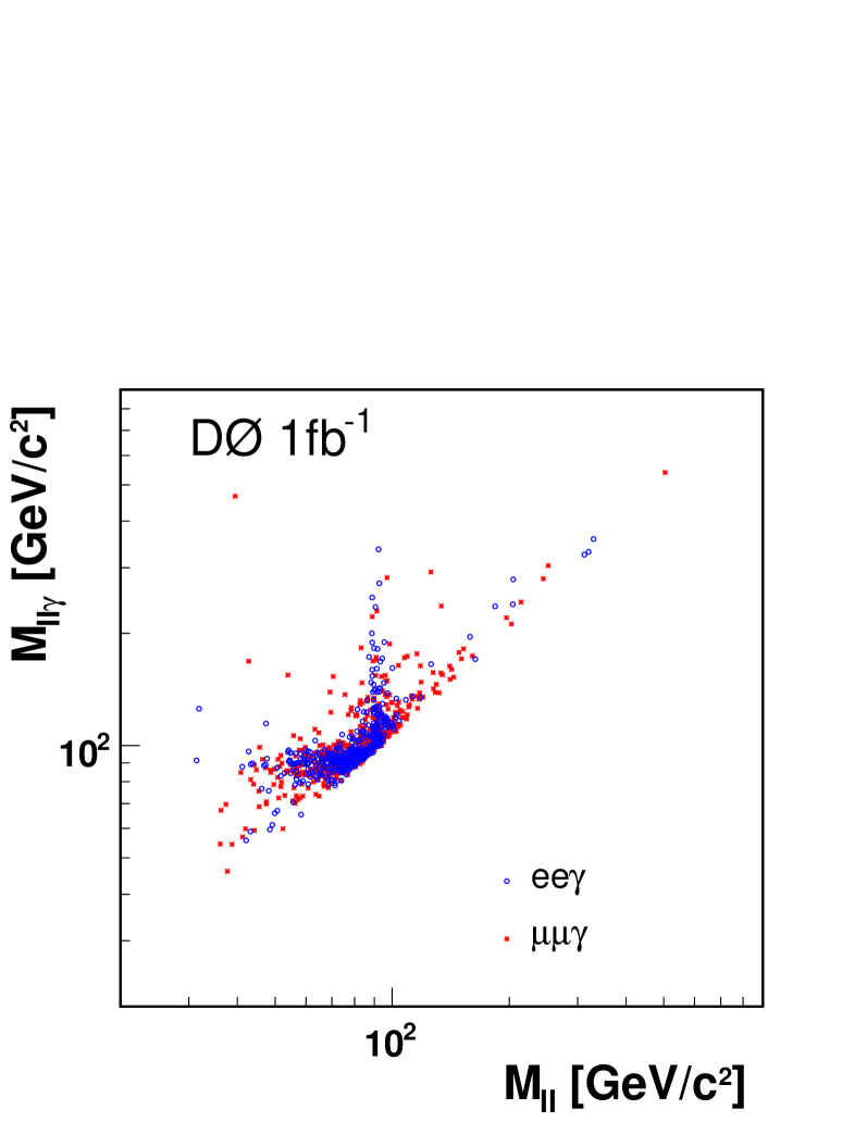
Figure 15: The three-body mass $M_{\ell\ell\gamma}$ versus the dilepton mass $M_{\ell\ell}$ for $Z\gamma$ candidate events in the D0 analysis [56]

Using $\int{\cal L}~{}dt=3.6~{}\rm{fb}^{-1}$, the D0 collaboration has observed (5.1$\sigma$) the $Z\gamma\rightarrow\nu\nu\gamma$ process for the first time at a hadron collider [58] and used these events to search for $Z\gamma\gamma$ and $ZZ\gamma$ couplings that are absent at tree-level in the SM. The experimental signature for $Z\gamma\rightarrow\nu\nu\gamma$ is a high energy photon and large $E\kern-6.00006pt\raise 0.43057pt\hbox{/}_{T}$. In the analysis, events are required to have a single photon candidate with $E_{T}>90$ GeV and $\mbox{$E\kern-6.00006pt\raise 0.43057pt\hbox{/}_{T}$}>70$ ${\rm GeV/c}$. The primary backgrounds are from $W\rightarrow e\nu$ and events unrelated to the collision in which muons from beam halo or cosmic rays produce energetic photons through bremsstrahlung. The $W\rightarrow e\nu$ is suppressed by removing events with high-$p_{T}$ tracks and the non-collision events are removing using available $z_{0}$ production information from the EM calorimeter and pre-shower detectors. A summary of the background estimates and observed events is shown in Tab. 8. The measured cross section is

$$\sigma(p\bar{p}\rightarrow Z\gamma+X)\times BR(Z\rightarrow\nu\nu)$$

$${}=32~{}\pm~{}9\rm{(stat.+syst.)}~{}\pm~{}2\rm{(lum.)}~{}\rm{fb}$$

for the photon $E_{T}>90$ GeV, consistent with the NLO cross section of $39~{}\pm~{}4$ fb [57].

	Number of events
$W\to e\nu$	$9.67\pm 0.30(\rm stat.)\pm 0.48(\rm syst.)$
non-collision	$5.33\pm 0.39(\rm stat.)\pm 1.91(\rm syst.)$
$W/Z$ + jet	$1.37\pm 0.26(\rm stat.)\pm 0.91(\rm syst.)$
$W\gamma$	$0.90\pm 0.07(\rm stat.)\pm 0.12(\rm syst.)$
Total background	$17.3\pm 0.6(\rm stat.)\pm 2.3(\rm syst.)$
$N_{\nu\bar{\nu}\gamma}^{\rm SM}$	$33.7\pm 3.4$
$N_{\rm obs}$	51

Table 8: Summary of background estimates, and the number of observed and SM predicted events for the D0 analysis of the $Z\gamma\rightarrow\nu\nu\gamma$ channel [58].

Both of the CDF and D0 $Z\gamma$ cross section measurements are consistent with the SM expectations at NLO. D0 searches for anomalous $Z\gamma\gamma$ and $ZZ\gamma$ couplings using the observed photon $E_{T}$ spectrum in the $Z\gamma\rightarrow\ell\ell\gamma$ [56] and $Z\gamma\rightarrow\nu\nu\gamma$ [58]. A LO simulation [43; 57] of the $Z\gamma$ signal is used with NLO corrections [57] applied to the photon $E_{T}$ spectrum. The observed photon $E_{T}$ spectrum along with the SM expectation and possible anomalous TGC scenarios for two channels is shown in Fig. 16. The $Z\gamma\rightarrow\ell\ell\gamma$ and $Z\gamma\rightarrow\nu\nu\gamma$ combined limits on the CP-conserving $Z\gamma\gamma$ and $ZZ\gamma$ couplings are shown in Fig. 17. The 1D combined limits at 95% CL are $|h_{30}^{\gamma}|<0.033$, $|h_{40}^{\gamma}|<0.0017$, $|h_{30}^{Z}|<0.033$, and $|h_{40}^{Z}|<0.0017$ for $\Lambda=1.5$ TeV.

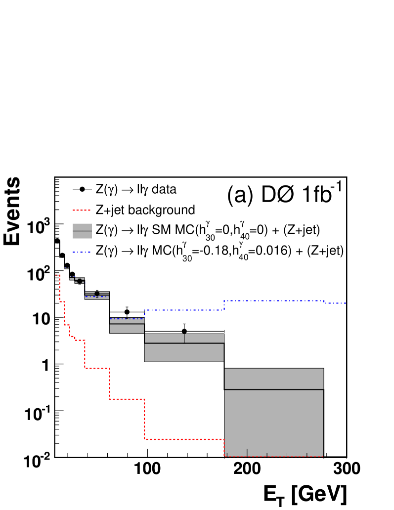
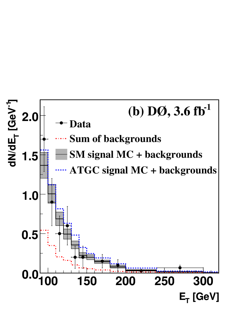
Figure 16: The observed photon $E_{T}$ spectrum along with the SM expectation and possible anomalous TGC scenarios for (a) $Z\gamma\rightarrow\ell\ell\gamma$ [56] and (b) $Z\gamma\rightarrow\nu\nu\gamma$ [58] channels.

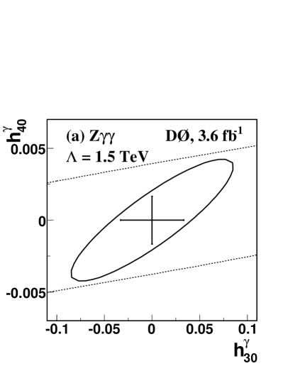
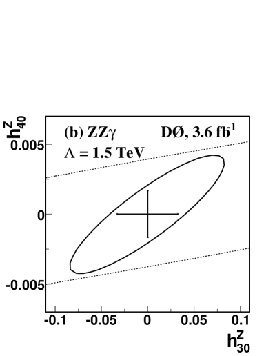
Figure 17: Two-dimensional bounds (ellipses) at 95% CL on CP-conserving (a) $Z\gamma\gamma$ and (b) $ZZ\gamma$ couplings. The crosses represent the one-dimensional bounds at the 95% CL setting all other couplings to zero. The dashed lines indicate the unitarity limits for $\Lambda=1.5$ TeV [58].

III.5.4 $WW$

Production of $W$ boson pairs in hadron (and lepton) collisions involves both the $WW\gamma$ and $WWZ$ couplings. First evidence for $W$ boson pair production was reported by CDF using Tevatron Run I data [59]. This process was later measured with greater significance by D0 and CDF using $\int{\cal L}~{}dt=224-252$ pb^-1 and $\int{\cal L}~{}dt=184$ pb^-1 respectively, from Run II of the Tevatron [60; 61]. At LEP, $WW$ production has been extensively studied and stringent limits on anomalous TGC were determined. At the Tevatron, much higher $WW$ invariant masses are probed compared to LEP because of the higher accessible energies. Also, the $WW$ final state is a promising discovery channel for the Higgs boson at both the Tevatron and the LHC. In hadron collisions, the production of $W$ boson pairs is most easily observed in the fully leptonic decay mode $WW\rightarrow\ell\nu\ell\nu$. The experimental signature of the $WW$ signal in leptonic decay is two isolated high $E_{T}$ charged leptons with opposite charge and large $E\kern-6.00006pt\raise 0.43057pt\hbox{/}_{T}$ from the neutrinos.

Both CDF and D0 have measured the $WW$ production cross section in fully-leptonic decay and use their data to search for anomalous $WW\gamma$ and $WWZ$ couplings. In both analyses, the dominant backgrounds are from $t\bar{t}$, Drell-Yan, other diboson decays, and $W$+jets where the jet fakes an isolated lepton. In the CDF analysis [62], $t\bar{t}$ is suppressed by requiring no reconstructed jets with $E_{T}>15$ GeV and $|\eta|<2.5$. In the D0 analysis [63], the $p_{T}$ of the $WW$ system, estimated from the observed charged lepton momenta and the $E\kern-6.00006pt\raise 0.43057pt\hbox{/}_{T}$, is required to be small ($<$20 ${\rm GeV/c}$ ($ee$), 25 ${\rm GeV/c}$ ($e\mu$), or 16 ${\rm GeV/c}$($\mu\mu$)) in order to suppress $t\bar{t}$ decays.

The strategy for measuring the cross section for $p\bar{p}\rightarrow WW+X$ differ between the CDF and D0 analyses. In the D0 analysis, the $WW$ signal yield is determined from counting the number of events in excess of the expected SM backgrounds using $\int{\cal L}~{}dt=1.1~{}\rm{fb}^{-1}$, as shown in Tab. 9. D0 measures

$$\sigma(p\bar{p}\rightarrow WW+X)$$

$${}=11.5~{}\pm~{}2.1\rm{(stat.+syst.)}~{}\pm~{}0.7\rm{(lum.)}~{}\rm{pb}$$

[63], in agreement with the NLO expectation of $12.0~{}\pm~{}0.7$ pb [64].

Process	$ee$		$e\mu$		$\mu\mu$
$Z/\gamma^{*}\to ee/\mu\mu$	0.27$\,\pm\,$	0.20	2.52$\,\pm\,$	0.56	0.76$\,\pm\,$	0.36
$Z/\gamma^{*}\to\tau\tau$	0.26$\,\pm\,$	0.05	3.67$\,\pm\,$	0.46	—
$t\bar{t}$	1.10$\,\pm\,$	0.10	3.79$\,\pm\,$	0.17	0.22$\,\pm\,$	0.04
$WZ$	1.42$\,\pm\,$	0.14	1.29$\,\pm\,$	0.14	0.97$\,\pm\,$	0.11
$ZZ$	1.70$\,\pm\,$	0.04	0.09$\,\pm\,$	0.01	0.84$\,\pm\,$	0.03
$W\gamma$	0.23$\,\pm\,$	0.16	5.21$\,\pm\,$	2.97	—
$W+\text{jet}$	6.09$\,\pm\,$	1.72	7.50$\,\pm\,$	1.83	0.12$\,\pm\,$	0.24
Multijet	0.01$\,\pm\,$	0.01	0.14$\,\pm\,$	0.13	—
$WW\to\ell\ell^{\prime}$	10.98$\,\pm\,$	0.59	39.25$\,\pm\,$	0.81	7.18$\,\pm\,$	0.34
$WW\to\ell\tau/\tau\tau\to\ell\ell^{\prime}$	1.40$\,\pm\,$	0.20	5.18$\,\pm\,$	0.29	0.71$\,\pm\,$	0.10
Total expected	23.46$\,\pm\,$	1.90	68.64$\,\pm\,$	3.88	10.79$\,\pm\,$	0.58
Data	22		64		14

Table 9: Numbers of signal and background events expected and number of events observed after the final event selection in each channel for the D0 $WW$ cross section measurement [63].

In the CDF analysis, the $WW$ signal yield is extracted from a fit to the distribution of a matrix element likelihood ratio ($LR_{WW}$) discriminant for events using $\int{\cal L}~{}dt=3.6~{}\rm{fb}^{-1}$. The events which are fit are required to pass relatively loose selection criteria as compared to the selection CDF would use for a cross section measurement based on the event yield alone. Tab. 10 shows the expected

Process	Events
$Z/\gamma^{*}$ (Drell-Yan)	79.8 $\pm$ 18.4
$WZ$	13.8 $\pm$ 1.9
$W\gamma$	91.7 $\pm$ 24.8
$W+1-$jet	112.7 $\pm$ 31.2
$ZZ$	20.7 $\pm$ 2.8
$t\bar{t}$	1.3 $\pm$ 0.2
Total Background	320.0 $\pm$ 46.8
$W^{+}W^{-}$	317.6 $\pm$ 43.8
Total Expected	637.6 $\pm$ 73.0
Data	654

Table 10: Expected number of signal ($WW$) and background events along with the total number of expected and observed events in the data for the CDF $WW$ cross section measurement [62].

number of signal and background events along with the observed events in the data used to fit for the signal. For each event passing the signal selection criteria, four matrix-element-based (ME) event probabilities are calculated corresponding to the production and decay processes $WW\rightarrow\ell\nu\ell\nu$, $ZZ\rightarrow\ell\ell\nu\nu$, $W+1-$jet $\rightarrow\ell\nu+$ 1-jet, and $W\gamma\rightarrow\ell\nu+\gamma$. In the latter two processes, the jet or $\gamma$ is assumed to have been reconstructed as a charged lepton candidate. The event probability for a process $X$ is given by

$$P_{X}(\vec{x})=\frac{1}{\langle\sigma\rangle}\int\frac{d\sigma(\vec{y})}{d\vec{y}}\;\epsilon(\vec{y})\;G(\vec{x},\vec{y})\;d\vec{y}$$ (7)

where $\vec{x}$ represents the observed lepton momenta and $E\kern-6.00006pt\raise 0.43057pt\hbox{/}_{T}$ vectors, $G(\vec{x},\vec{y})$ is a transfer function representing the detector resolution, and $\epsilon(\vec{y})$ is an efficiency function parametrized by $\eta$ which quantifies the probability for a particle to be reconstructed as a lepton. The differential cross section $\frac{d\sigma(\vec{y})}{d\vec{y}}$ is calculated using leading-order matrix elements from the mcfm program [64] and integrated over all possible true values of the final state particle 4-vectors $\vec{y}$. The normalization factor $\langle\sigma\rangle$ is determined from the leading-order cross section and detector acceptance for each process. These event probabilities are combined into a likelihood ratio

$$LR_{WW}=\frac{P_{WW}}{P_{WW}+\sum_{j}k_{j}P_{j}},$$ (8)

where $j=\{ZZ,$ $W+1-$jet, $W\gamma\}$ and $k_{j}$ is the relative fraction of the expected number of events for the $j$-th process such that $\sum_{j}k_{j}=1$. The templates of the $LR_{WW}$ distribution are created for signal and each background process given in Tab. 10.

A binned maximum likelihood is used to extract the $WW$ production cross section from the shape and normalization of the $LR_{WW}$ templates. The likelihood is formed from the Poisson probabilities of observing $n_{i}$ events in the $i$-th bin when $\mu_{i}$ are expected. Variations corresponding to the systematic uncertainties described previously are included as normalization parameters for signal and background, constrained by Gaussian terms. The likelihood is given by

$$\mathcal{L}=\left(\prod_{i}\frac{\mu_{i}^{n_{i}}e^{-\mu_{i}}}{n_{i}!}\right)\cdot\prod_{c}e^{-\frac{S_{c}^{2}}{2}}$$ (9)

where

$$\mu_{i}=\sum_{k}\alpha_{k}\left[\prod_{c}(1+f^{c}_{k}S_{c})\right](N^{Exp}_{k})_{i},$$ (10)

$f^{c}_{k}$ is the fractional uncertainty for the process $k$ due to the systematic $c$, and $S_{c}$ is a floating parameter associated with the systematic uncertainty $c$. The correlations of systematic uncertainties between processes are accounted for in the definition of $\mu_{i}$. The expected number of events from process $k$ in the $i$-th bin is given by $(N^{Exp}_{k})_{i}$. The parameter $\alpha_{k}$ is an overall normalization parameter for process $k$ and is fixed to unity for all processes other than $WW$, for which it is freely floating. The likelihood is maximized with respect to the systematic parameters $S_{c}$ and $\alpha_{WW}$. The $WW$ cross section is then given by the fitted value of $\alpha_{WW}$ multiplied by $\sigma^{NLO}(p\bar{p}\to WW)$.

The fit to the data of the signal and sum of the individually fitted background templates is show in Fig. 18. The measured $WW$ production cross section is

$$\sigma(p\bar{p}\rightarrow WW+X)$$

$${}=12.1~{}\pm~{}0.9\rm{(stat.)}~{}^{1.6}_{-1.4}\rm{(syst.)}~{}\rm{pb}$$

[62] in agreement with the NLO theoretical expectation of $11.7~{}\pm~{}0.7$ pb [64].

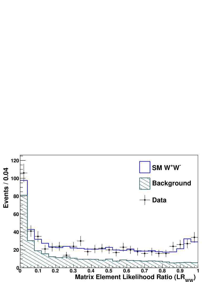
Figure 18: The $LR_{WW}$ distributions for the signal ($W^{+}W^{-}$) and background processes after a maximum likelihood fit to the data for the CDF $WW$ cross section measurement [62].

Both of the CDF and D0 $WW$ cross section measurements are consistent with the SM expectations at NLO. CDF searches for anomalous $WW\gamma$ and $WWZ$ couplings using the observed leading charged lepton $p_{T}$ spectrum (see Fig. 19). In the D0 analysis, the subleading (trailing) lepton $p_{T}$ is also included in a 2D histogram with the leading lepton $p_{T}$ to constrain possible anomalous couplings (see Fig. 20 for the 1D projections).

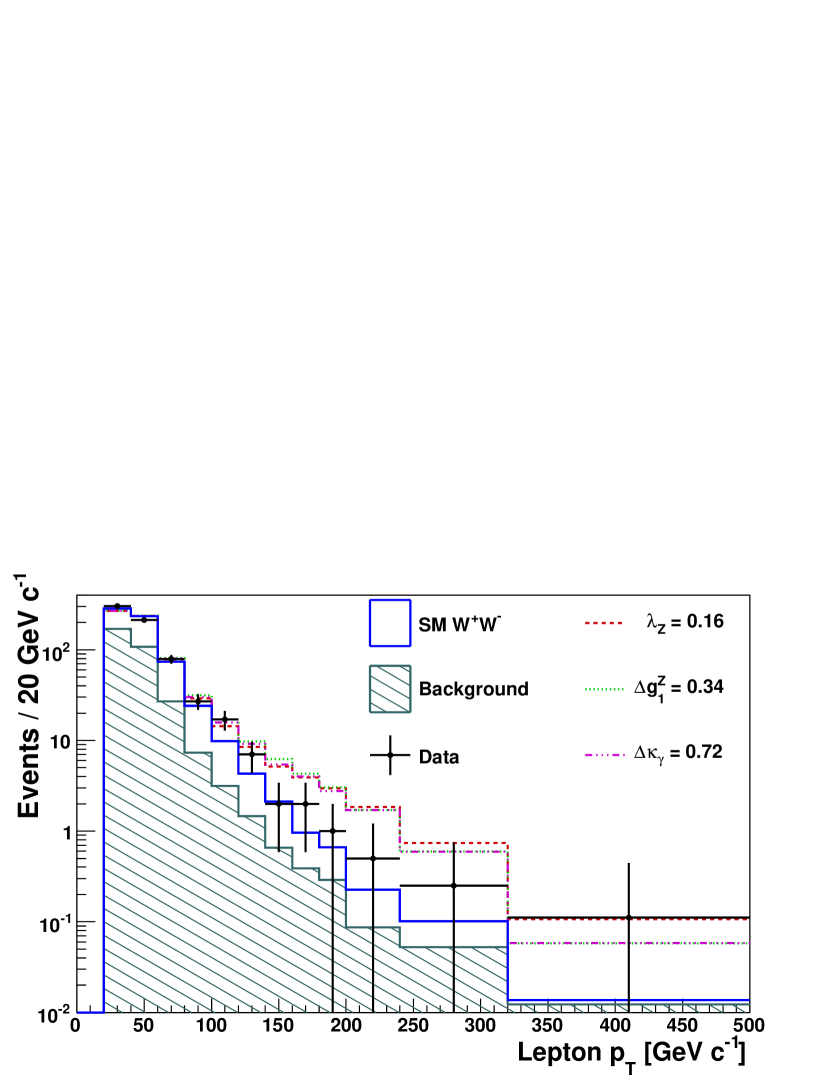
Figure 19: Leading-lepton $p_{T}$ distribution for data compared to the SM expectation for the CDF $WW\rightarrow\ell\nu\ell\nu$ analysis [62]. Also shown is how the expectation would be modified by anomalous couplings near the observed limits.

Figure 20: Distributions of the (a) leading and (b) trailing lepton $p_{T}$ for the D0 $WW\rightarrow\ell\nu\ell\nu$ analysis [63]. Data are compared to estimated signal, $\sigma(WW)=12$ pb, and background sum.

There are several ways to relate the $WW\gamma$ and $WWZ$ couplings in the presence of new physics. This is a convenient prescription to reduce the number of parameters since $WW$ production involves both $WW\gamma$ and $WWZ$ couplings. Enforcing $SU(2)_{L}\otimes U(1)_{Y}$ symmetry introduces two relationships between the remaining parameters: $\kappa_{Z}=g_{1}^{Z}-(\kappa_{\gamma}-1)\mathrm{tan}^{2}\theta_{W}$ and $\lambda_{Z}=\lambda_{\gamma}$, reducing the number of free parameters to three [5; 6]. Alternatively, enforcing equality between the $WW\gamma$ and $WWZ$ vertices ($WW\gamma$=$WWZ$) such that $\kappa_{\gamma}=\kappa_{Z}$, $\lambda_{\gamma}=\lambda_{Z}$, and $g^{Z}_{1}=1$ reduces the number of free parameters to two.

In the D0 analysis, the one-dimensional 95% CL limits for $\Lambda=2$ TeV are determined to be $-0.54<\Delta\kappa_{\gamma}<0.83$, $-0.14<\lambda_{\gamma}=\lambda_{Z}<0.18$, and $-0.14<\Delta g_{1}^{Z}<0.30$ under the $SU(2)_{L}\otimes U(1)_{Y}$-conserving constraints, and $-0.12<\Delta\kappa_{\gamma}=\Delta\kappa_{Z}<0.35$, with the same $\lambda$ limits as above, under the $WW\gamma$=$WWZ$ constraints. One- and two-dimensional 95% CL limits are shown in Fig. 21. In the CDF analysis, only 1D limits on the anomalous coupling parameters under the assumption of $SU(2)_{L}\otimes U(1)_{Y}$ invariance are reported. The expected and observed 95% confidence limits are shown in Tab. 11 where it is evident that the limits are weaker than expected. The probability of observing these limits in the presence of only SM $WW$ production ranges from 7.1% to 7.6% depending on the coupling parameters ($\lambda_{Z}$, $\Delta\kappa_{\gamma}$, $\Delta g_{1}^{Z}$) and are consistent with a statistical fluctuation of SM physics.

Figure 21: One and two-dimensional 95% CL limits for the D0 $WW\rightarrow\ell\nu\ell\nu$ analysis [63] when enforcing $SU(2)_{L}\otimes U(1)_{Y}$ symmetry at $\Lambda=2$ TeV, for (a) $\Delta\kappa_{\gamma}$ vs. $\lambda_{\gamma}$, (b) $\Delta\kappa_{\gamma}$ vs. $\Delta g_{1}^{Z}$, and (c) $\lambda_{\gamma}$ vs. $\Delta g_{1}^{Z}$, each when the third free coupling is set to its SM value; limits when enforcing the $WW\gamma$=$WWZ$ constraints are shown in (d). The curve represents the two-dimensional 95% CL contour and the ticks along the axes represent the one-dimensional 95% CL limits. An asterisk ($+\times$) marks the point with the highest likelihood in the two-dimensional plane.

		$\Lambda$ (TeV)	$\lambda_{\gamma}=\lambda_{Z}$	$\Delta\kappa_{\gamma}$	$\Delta g_{1}^{Z}$
Expected		1.5	(-0.05,0.07)	(-0.23,0.31)	(-0.09,0.17)
Observed		1.5	(-0.16,0.16)	(-0.63,0.72)	(-0.24,0.34)
Expected		2.0	(-0.05,0.06)	(-0.20,0.27)	(-0.08,0.15)
Observed		2.0	(-0.14,0.15)	(-0.57,0.65)	(-0.22,0.30)

Table 11: Expected and observed limits from the CDF $WW\rightarrow\ell\nu\ell\nu$ analysis searching for anomalous TGCs assuming two different values of the form factor scale $\Lambda$ [62]. For each coupling limit set, the two other couplings are fixed at their SM values. Values of the couplings outside of the given observed range are excluded at the 95% confidence level (CL).

III.5.5 $WZ$

The $WZ$ final state is not available in $e^{+}e^{-}$ collisions at LEP but can be produced in $p\overline{p}$ collisions at the Tevatron. The study of associated production of a $W$ and $Z$ boson is important for a number of reasons. The production of $WZ$ involves the $WWZ$ TGC as shown in the s-channel diagram in Fig. 22. Unlike $WW$ production which involves a combination of the $WW\gamma$ and $WWZ$ couplings such that assumptions regarding their relation must be invoked to interpret any anomalies observed in the data, the $WZ$ production characteristics can be used to make a model-independent test of the SM $WWZ$ coupling. Stated slightly differently, in $WZ$ production measurements, a direct measure of the $WZ$ coupling independent of the $W\gamma$ coupling can be made and compared to the SM predictions. The fully-leptonic decay mode of $WZ$ provides a clean SM trilepton signal which is analogous to the so-called golden mode for discovering supersymmetry (SUSY) at the Tevatron via chargino-neutralino production (${\tilde{\chi}}_{1}^{\pm}{\tilde{\chi}}_{2}^{0}$) and decay. Therefore, an observation of the SM $WZ$ trilepton signal represents an important experimental milestone in demonstrating sensitivity to the SUSY golden mode and other new physics signatures in multileptons.

Figure 22: Leading order (a) t-channel and (b) s-channel diagrams for $WZ$ production at the Tevatron

Prior to the start of Run II at the Tevatron, $WZ$ production had not been observed. The next-to-leading order (NLO) $WZ$ cross section prediction for $p\overline{p}$ collisions at $\sqrt{s}=1.96~{}{\rm TeV}$ is 3.7 $\pm$ 0.3 pb [64]. In October 2006, $WZ$ production was first observed by the CDF Collaboration in the three charged lepton + $E\kern-6.00006pt\raise 0.43057pt\hbox{/}_{T}$ final state using 1.1$~{}\rm{fb}^{-1}$ of integrated luminosity [65]. The most sensitive previous search for $WZ$ production was reported by the $D0$ Collaboration using $\int{\cal L}~{}dt=0.3\ {\rm fb}^{-1}$, where three $WZ\rightarrow\ell^{\prime}\nu_{\ell^{\prime}}\ell\ell$ candidates were found [66]. The observed candidates had a probability of 3.5% to be due to background fluctuations, corresponding to $\sigma(WZ)<13.3$ pb at 95% CL. The D0 collaboration published an update to [66] with additional data to measure the $WZ$ production cross section and search for anomalous $WWZ$ couplings [67].

As with other diboson processes, the signal for $WZ$ production is most easily measured in fully-leptonic decay. The experimental signature of $WZ$ production is three isolated high $E_{T}$ charged leptons, at least two of which having the same flavor and opposite charge with invariant mass consistent with decay of a $Z$ boson, and large $E\kern-6.00006pt\raise 0.43057pt\hbox{/}_{T}$ consistent with a neutrino from $W$ decay. To observe $WZ$ in fully-leptonic decay, high acceptance for charged leptons is required since all three must be detected to suppress backgrounds from larger cross section processes. In the CDF analysis [65], a novel lepton identification strategy was developed to maximize charged lepton acceptance while keeping the backgrounds comparatively low by exploiting the charge and flavor correlation of identified leptons in the events. The standard electron and muon identification was combined with forward electron candidates beyond the tracking acceptance and a “track-only” lepton category consisting of high-quality tracks that neither project to the fiducial regions of the calorimeters nor are identified as muons by the muon chambers. Due to the lack of calorimeter information, electrons and muons cannot be reliably differentiated for this category, and are therefore treated as having either flavor in the $WZ$ candidate selection. For forward electrons without a matched track, both charge hypotheses are considered when forming $WZ$ candidates, since the charge is determined from the track curvature.

Other SM processes that can lead to three high-$p_{T}$ leptons include dileptons from the Drell-Yan $Z/\gamma^{*}$ process (DY), with an additional lepton from a photon conversion ($Z\gamma$) or a misidentified jet ($Z$+jets) in the event; $ZZ$ production where only three leptons are identified and the unobserved lepton results in $E\kern-6.00006pt\raise 0.43057pt\hbox{/}_{T}$; and a small contribution from $t\overline{t}\rightarrow WbW\bar{b}$, where two charged leptons result from the $W$ boson decays and one or more from decay of the $b$-quarks. Except for $t\overline{t}$, these backgrounds are suppressed by requiring $\mbox{$E\kern-6.00006pt\raise 0.43057pt\hbox{/}_{T}$}>25$ GeV in the event, consistent with the unobserved neutrino from the leptonic decay of a $W$ boson.

Using $\int{\cal L}~{}dt=1.1~{}\rm{fb}^{-1}$, 16 events with an expected background of 2.7 $\pm$ 0.4 events are observed in the CDF analysis, as shown in Fig. 12. This corresponds to a 6.0$\sigma$ observation of $WZ$ production when $E\kern-6.00006pt\raise 0.43057pt\hbox{/}_{T}$ shape information is included. The measured cross section is

$$\sigma(p\bar{p}\rightarrow WZ+X)=5.0^{+1.8}_{-1.6}~{}\rm{(stat.+syst.)}~{}\rm{pb},$$

consistent with the NLO expectation. Fig. 23 shows some important kinematic distributions for the 16 $WZ$ candidates, which are in good agreement with the SM.

Source	Expectation $\pm$ Stat $\pm$ Syst $\pm$ Lumi
$Z$+jets	1.21 $\pm$ 0.27 $\pm$ 0.28 $\pm$  $-$
$ZZ$	0.88 $\pm$ 0.01 $\pm$ 0.09 $\pm$ 0.05
$Z\gamma$	0.44 $\pm$ 0.05 $\pm$ 0.15 $\pm$ 0.03
$t\bar{t}$	0.12 $\pm$ 0.01 $\pm$ 0.02 $\pm$ 0.01
Total Background	2.65 $\pm$ 0.28 $\pm$ 0.33 $\pm$ 0.09
$WZ$	9.75 $\pm$ 0.03 $\pm$ 0.31 $\pm$ 0.59
Total Expected	12.41 $\pm$ 0.28 $\pm$ 0.45 $\pm$ 0.67
Observed	16

Table 12: Expected number of events in the signal region for $WZ$ and the background contributions for the CDF $WZ\rightarrow\ell\ell\ell\nu$ analysis [65]. “Lumi” refers to the integrated luminosity uncertainty, which is absent for the $Z$+jets because it is determined from the same data set.

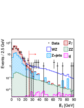
Figure 23: Distributions for $WZ$ candidates of (a) the $E\kern-6.00006pt\raise 0.43057pt\hbox{/}_{T}$ (b) the dilepton invariant mass for the same-flavor opposite-sign dilepton pair closest to the $Z$ mass, and (c) the $W$ transverse mass calculated from the remaining lepton and the $E\kern-6.00006pt\raise 0.43057pt\hbox{/}_{T}$, for the CDF $WZ\rightarrow\ell\ell\ell\nu$ analysis [65]. In (a) and (b), the arrows indicate the signal region.

In the D0 analysis [67], events with three reconstructed, isolated charged leptons (electrons or muons) and $\mbox{$E\kern-6.00006pt\raise 0.43057pt\hbox{/}_{T}$}>20$ GeV were used to measure the $WZ$ production cross section and search for anomalous $WWZ$ couplings using the observed $Z$ boson $p_{T}$ ($p_{T}^{Z}$) distribution. Each $WZ$ candidate event must contain a like-flavor lepton pair with invariant mass close to the $Z$ boson mass. For $eee$ and $\mu\mu\mu$ decay channels, the lepton pair with invariant mass closest to that of the $Z$ boson mass is chosen to define the $Z$ boson daughter particles. Using $\int{\cal L}~{}dt=1.0~{}\rm{fb}^{-1}$, a total of 13 $WZ$ candidates are observed with $4.5\pm 0.6$ expected background events and $9.2\pm 1.0$ expected $WZ$ signal events, corresponding to a 3.0$\sigma$ signal significance. The breakdown by trilepton flavor classification for both the CDF and D0 analyses is shown in Tab. 13. Fig. 24 shows ${\hbox{$E$\kern-6.00006pt\lower-0.43057pt\hbox{/}}}_{T}$ versus the dilepton invariant mass for the background, the expected $WZ$ signal, and the data, including the candidates for the D0 analysis. The $WZ$ production cross section measured by D0 is

$$\sigma(p\bar{p}\rightarrow WZ+X)=2.7^{+1.7}_{-1.3}~{}\rm{(stat.+syst.)}~{}\rm{pb},$$

where the $\pm 1\sigma$ uncertainties are the $68\%$ CL limits from the minimum of the negative log likelihood. The uncertainty is dominated by the statistics of the number of observed events.

Flavor	CDF Analysis		D0 Analysis
Classification	Expected	Data	Expected	Data
$e$ $e$ $e$	2.7 $\pm$ 0.2	6	3.5 $\pm$ 0.2	2
$e$ $e$ $\mu$	2.0 $\pm$ 0.2	0	2.7 $\pm$ 0.2	1
$e$ $\mu$ $\mu$	1.5 $\pm$ 0.1	1	4.2 $\pm$ 0.5	8
$\mu$ $\mu$ $\mu$	1.2 $\pm$ 0.1	1	3.4 $\pm$ 0.4	2
$e$ $e$ $\ell_{t}$	2.0 $\pm$ 0.2	5	$-$	$-$
$e$ $\mu$ $\ell_{t}$	1.3 $\pm$ 0.1	2	$-$	$-$
$\mu$ $\mu$ $\ell_{t}$	1.1 $\pm$ 0.1	1	$-$	$-$
$e$ $\ell_{t}$ $\ell_{t}$	0.5 $\pm$ 0.1	0	$-$	$-$
$\mu$ $\ell_{t}$ $\ell_{t}$	0.2 $\pm$ 0.1	0	$-$	$-$

Table 13: Summary of the expected and observed yields for the CDF [65] and D0 [67] $WZ\rightarrow\ell\ell\ell\nu$ analyses. In the classification column, $\ell_{t}$ denotes a track-only lepton candidate having unknown flavor which is only relevant for the CDF analysis.

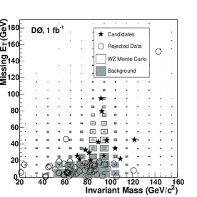
Figure 24: ${\hbox{$E$\kern-6.00006pt\lower-0.43057pt\hbox{/}}}_{T}$ versus dilepton invariant mass of $WZ\rightarrow\ell\ell\ell\nu$ candidate events in the D0 $WZ$ analysis[67]. The open boxes represent the expected $WZ$ signal. The gray boxes represent the sum of the estimated backgrounds. The black stars are the data that survive all selection criteria. The open circles are data that fail either the dilepton invariant mass criterion or have $\mbox{$E\kern-6.00006pt\raise 0.43057pt\hbox{/}_{T}$}<20$ GeV.

The three $CP$-conserving $WWZ$ coupling parameters $\lambda_{Z}$, $\Delta g^{Z}_{1},$ and $\Delta\kappa_{Z}$ are constrained in the D0 analysis by comparing the measured cross section and $p_{T}^{Z}$ distribution to models with anomalous couplings. A comparison of the observed $Z$ boson $p_{T}$ distribution with predictions from Monte Carlo simulation is shown in Fig. 25. Tab. 14 presents the one-dimensional 95% CL limits on $\lambda_{Z}$, $\Delta g^{Z}_{1}$ and $\Delta\kappa_{Z}$. Fig. 26 presents the two-dimensional 95% CL limits under the assumption $\Delta g^{Z}_{1}=\Delta\kappa_{Z}$ for $\Lambda=2$ TeV.

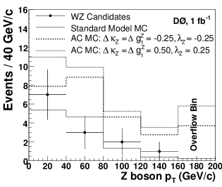
Figure 25: The reconstructed $Z$ boson $p_{T}$ of the $WZ$ candidate events for the D0 $WZ\rightarrow\ell\ell\ell\nu$ analysis [67]. The solid histogram is the expected sum of signal and background for the case of the $WWZ$ coupling parameters set to their SM values. The dotted and double dotted histograms are the expected sums of signal and background for two different cases of anomalous $WWZ$ coupling parameter values.

$\Lambda=1.5\text{~{}TeV}$	$\Lambda=2.0\text{~{}TeV}$
$-0.18<\lambda_{Z}<0.22$	$-0.17<\lambda_{Z}<0.21$
$-0.15<\Delta g^{Z}_{1}<0.35$	$-0.14<\Delta g^{Z}_{1}<0.34$
$-0.14<\Delta\kappa_{Z}=\Delta g^{Z}_{1}<0.31$	$-0.12<\Delta\kappa_{Z}=\Delta g^{Z}_{1}<0.29$

Table 14: One-dimensional 95% CL intervals on $\lambda_{Z}$, $\Delta g^{Z}_{1}$, and $\Delta\kappa_{Z}$ for two sets of form factor scale, $\Lambda$, for the D0 $WZ\rightarrow\ell\ell\ell\nu$ analysis [67].

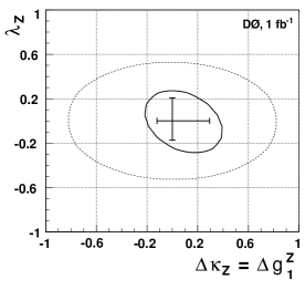
Figure 26: Two-dimensional 95% CL contour limit in $\Delta g_{1}^{Z}=\Delta\kappa_{Z}$ versus $\Delta\lambda_{Z}$ space (inner contour) for the D0 $WZ\rightarrow\ell\ell\ell\nu$ analysis [67]. The form factor scale for this contour is $\Lambda=2$ TeV. The physically allowed region (unitarity limit) is bounded by the outer contour. The cross hairs are the 95% CL one-dimensional limits.

III.5.6 $ZZ$

The production of $Z$ pairs is predicted within the SM to have the smallest cross section among the diboson processes. It has been been observed in $e^{+}e^{-}$ collisions at LEP [68], but not in hadron collisions as of the start of the Tevatron Run II. As a window to new physics, $ZZ$ production is particularly interesting because of the absence of $ZZ\gamma$ and $ZZZ$ couplings in the SM (see Fig. 27), and because of the very low backgrounds in the four charged-lepton channel. Higgs boson decay can contribute to $ZZ$ production; however, this channel is generally not competitive with $H\rightarrow WW^{(*)}$ as a discovery channel at the Tevatron collision energy and integrated luminosity.

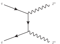
Figure 27: Leading order diagram for $ZZ$ production at the Tevatron. The s-channel diagram involving the neutral TGC is absent in the SM.

As is the case in for $WW$ and $WZ$ production, the $ZZ$ state is most easily observed in the fully leptonic mode at a hadron collider. The $ZZ\rightarrow\ell\ell\ell\ell$ process is rare but predicted to be nearly background free in the SM, with $Z$+jets (jets reconstructed as charged leptons) as the only non-negligible background. Having large total charged lepton acceptance in the experiments is crucial due to the high lepton multiplicity in the final state. The $ZZ\rightarrow\ell\ell\nu\nu$ process can also contribute sensitivity to the search for $ZZ$ production although it suffers from large continuum $WW$ backgrounds. The full SM process is $p\overline{p}\rightarrow Z/\gamma^{*}~{}Z/\gamma^{*}$, where the two $Z/\gamma^{*}$ interfere with one another. For brevity, we denote $Z/\gamma^{*}~{}Z/\gamma^{*}$ as $ZZ$ throughout and indicate the dilepton invariant mass range(s), where applicable. The next-to-leading order (NLO) $ZZ$ cross section for $p\overline{p}$ collisions at $\sqrt{s}=1.96~{}{\rm TeV}$ is 1.4 $\pm$ 0.1 pb in the zero-width $Z$ boson approximation [64].

Using $\int{\cal L}~{}dt=1~{}\rm{fb}^{-1}$, the D0 Collaboration searched for $ZZ\rightarrow\ell\ell\ell\ell$ production and set a limit on the cross section of $\sigma(ZZ)$ $<$ 4.4 pb at 95% CL [69]. They constrain possible $ZZ\gamma$ and $ZZZ$ couplings based on the observed four lepton yield with the added requirement that $M(\ell\ell)>50\;(70)$ for electrons (muons). The value of the cut was chosen based on the dilepton invariant mass resolution. This lower $M(\ell\ell)$ requirement was included because the Monte Carlo generator [44] used to constrain possible anomalous couplings does not include contributions from off-shell $Z$ bosons. Without the $M(\ell\ell)$ cut, one $\mu\mu ee$ event is observed in the data. This event is removed by the $M(\ell\ell)$ cut used to constrain anomalous couplings. 1D and 2D limits on anomalous $ZZ\gamma$ and $ZZZ$ couplings are determined using $\Lambda=1.2$ TeV. The 95% CL 1D limits are $-0.28<f_{40}^{Z}<0.28$, $-0.26<f_{40}^{\gamma}<0.26$, $-0.31<f_{50}^{Z}<0.29$, and $-0.30<f_{50}^{\gamma}<0.28$. The 95% CL 2D contours $f_{40}^{\gamma}$ vs. $f_{40}^{Z}$, $f_{40}^{\gamma}$ vs. $f_{50}^{\gamma}$, $f_{40}^{Z}$ vs. $f_{50}^{Z}$, and $f_{50}^{\gamma}$ vs. $f_{50}^{Z}$ are shown in Fig. 28.

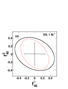
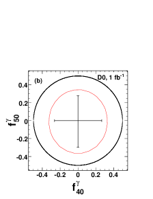
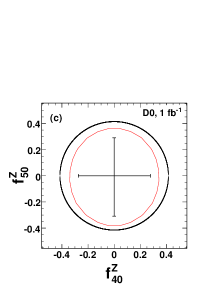
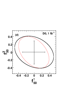
Figure 28: Limits on anomalous couplings for $\Lambda=1.2$ TeV for the D0 $ZZ\rightarrow\ell\ell\ell\ell$ analysis [69]: (a) $f_{40}^{\gamma}$ vs. $f_{40}^{Z}$, (b) $f_{40}^{\gamma}$ vs. $f_{50}^{\gamma}$, (c) $f_{40}^{Z}$ vs. $f_{50}^{Z}$, and (d) $f_{50}^{\gamma}$ vs. $f_{50}^{Z}$, assuming in each case that the other two couplings are zero. The inner and outer curves are the $95\%$ CL two-degree of freedom exclusion contour and the constraint from the unitarity condition, respectively. The inner cross hairs are the $95\%$ CL one-degree of freedom exclusion limits.

The CDF Collaboration uses $\int{\cal L}~{}dt=1.9~{}\rm{fb}^{-1}$ to search for $ZZ$ production in a combination of the $ZZ\rightarrow\ell\ell\ell\ell$ and $ZZ\rightarrow\ell\ell\nu\nu$ channels [70]. To maximize the acceptance, lepton candidates are constructed out of all reconstructed tracks and energy clusters in the EM section of the calorimeter. This is done with the same lepton identification criteria used in a previous CDF measurement of $WZ$ production [65]. The $ZZ\rightarrow\ell\ell\ell\ell$ candidates are selected from events with exactly four charged-lepton candidates and at least two same-flavor, opposite-sign lepton pairs are required for the event to be accepted. As in the $WZ$ analysis, trackless electrons are considered to have either charge, and track-only leptons either flavor. One pair must have invariant mass $M_{\ell^{+}\ell^{-}}$ in the range [76, 106] ${\rm GeV/c}^{2}$, while the requirement for the other pair is extended to [40, 140] ${\rm GeV/c}^{2}$ to increase the acceptance for off-shell $Z$ decays.

The $ZZ\rightarrow\ell\ell\ell\ell$ candidate events are separated into two exclusive categories based on whether or not they contain at least one forward electron without a track. This is done because the background from $Z\gamma$+jets is much larger in candidates with a forward trackless electron. The expected signal, expected background, and observed yields are shown in Tab. 15.

	Candidates without a	Candidates with a
Category	trackless electron	trackless electron
$ZZ$	1.990 $\pm$ 0.013 $\pm$ 0.210	0.278 $\pm$ 0.005 $\pm$ 0.029
$Z$+jets	${0.014}^{+0.010}_{-0.007}\pm 0.003$	${0.082}^{+0.089}_{-0.060}\pm 0.016$
Total	$2.004^{+0.016}_{-0.015}\pm 0.210$	$0.360^{+0.089}_{-0.060}\pm 0.033$
Observed	2	1

Table 15: Expected and observed number of $ZZ\rightarrow\ell\ell\ell\ell$ candidate events for the CDF $ZZ$ analysis [70]. The first uncertainty is statistical and the second one is systematic.

The $ZZ\rightarrow\ell\ell\nu\nu$ candidates are selected from events with exactly two oppositely-charged lepton candidates excluding events with forward electrons without a track which are contaminated by large $W\gamma$ backgrounds. Aside from $ZZ$ production, other SM processes that can lead to two high-$p_{T}$ leptons include events from DY, a $W$ decay with photon ($W\gamma$) or jet ($W$+jets) misidentified as a lepton; and $t\overline{t}$, $WW$, and $WZ$ production.

There are 276 events after the event selection (which contains a specialized high $E\kern-6.00006pt\raise 0.43057pt\hbox{/}_{T}$ to suppress primarily $DY$) of which only $14\pm 2$ are expected to be from the $ZZ\rightarrow\ell\ell\nu\nu$ process in the SM. Approximately half of the yield is expected to be due to the $WW$ process. However, $ZZ\rightarrow\ell\ell\nu\nu$ and $WW$ have different kinematic properties which are exploited to statistically separate the contribution of these two processes to the data. The approach used by CDF is identical to that used in the $WW$ cross section measurement described in Section III.5.4. An event-by-event probability density is calculated for the observed lepton momenta and $E\kern-6.00006pt\raise 0.43057pt\hbox{/}_{T}$ using leading order calculations of the differential decay rate for the processes [64]. A likelihood ratio discriminant $LR$ is formed which is the signal probability divided by the sum of signal and background probabilities $LR=P_{ZZ}/(P_{ZZ}+P_{WW})$. The distribution of $\log_{10}(1-LR)$ for the data compared to the summed signal and background expectation is shown in Fig. 29.

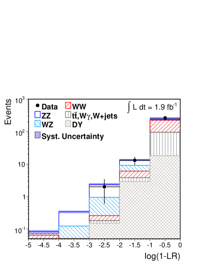
Figure 29: Distribution of the discriminating variable $\log_{10}(1-LR)$ for the CDF $ZZ\rightarrow\ell\ell\nu\nu$ search [70].

The $ZZ\rightarrow\ell\ell\ell\ell$ and $ZZ\rightarrow\ell\ell\nu\nu$ results were combined through a likelihood fit which includes the two 4-lepton bins and the $\log_{10}(1-LR)$ distribution for the dileptons. The p-value for the $ZZ\rightarrow\ell\ell\nu\nu$ alone is 0.12 and the combined p-value is $5.1\times 10^{-6}$ corresponding to a significance equivalent to 4.4 standard deviations. The $ZZ$ cross-section is obtained by fitting the data for the fraction of the expected SM yield in the full acceptance and scaling the zero-width $Z$ boson approximation cross-section by that fraction. The measured cross section is $\sigma(p\overline{p}\rightarrow ZZ)=1.4^{+0.7}_{-0.6}~{}\mathrm{pb},$ consistent with the SM expectation. This is the first evidence of a $ZZ$ signal with greater than 4$\sigma$ significance in hadron collisions.

The D0 Collaboration uses $\int{\cal L}~{}dt=1.7~{}\rm{fb}^{-1}$ to search for $ZZ$ production in the $ZZ\rightarrow\ell\ell\ell\ell$ channel [71]. This analysis follows up the analysis from [69] using more data and tighter dilepton invariant mass requirements but does not explicitly search for anomalous couplings. Four lepton events are selected using identified muons with $|\eta|<2$ and electrons that are either central ($|\eta<1.1$) or forward $1.5<|\eta|<3.2$. It is required that one pair have the same flavor with invariant mass $>70$ ${\rm GeV/c}^{2}$ and another pair have invariant mass $>50$ ${\rm GeV/c}^{2}$.

Tab. 16 summarizes the expected signal and background contributions to each subchannel, as well as the number of candidate events in data. The total signal and background expectations are $1.89\pm 0.08$ events and $0.14^{+0.03}_{-0.02}$ events, respectively. A total of three candidate events is observed, with two in the $4e_{4C}$ subchannel (“C” refers to the number of central leptons) and one in the $4\mu$ subchannel. Fig. 30 shows the distribution of the four lepton invariant mass for data and for the expected signal and background.

Subchannel	$4e_{2C}$	$4e_{3C}$	$4e_{4C}$	$4\mu$	$2\mu 2e_{0C}$	$2\mu 2e_{1C}$	$2\mu 2e_{2C}$
Luminosity (fb-1)	$1.75\pm 0.11$	$1.75\pm 0.11$	$1.75\pm 0.11$	$1.68\pm 0.10$	$1.68\pm 0.10$	$1.68\pm 0.10$	$1.68\pm 0.10$
Signal	$0.084\pm 0.008$	$0.173\pm 0.015$	$0.140\pm 0.012$	$0.534\pm 0.043$	$0.058^{+0.007}_{-0.006}$	$0.352\pm 0.040$	$0.553^{+0.045}_{-0.044}$
$Z(\gamma)$+jets	$0.030^{+0.009}_{-0.008}$	$0.018^{+0.008}_{-0.007}$	$0.002^{+0.002}_{-0.001}$	$0.0003\pm 0.0001$	$0.03^{+0.02}_{-0.01}$	$0.05\pm 0.01$	$0.008^{+0.004}_{-0.003}$
$t\bar{t}$	–	–	–	–	$0.0012^{+0.0016}_{-0.0009}$	$0.005\pm 0.002$	$0.0007^{+0.0009}_{-0.0005}$
Observed events	0	0	2	1	0	0	0

Table 16: The integrated luminosity, expected number of signal ($Z/\gamma^{*}$ $Z/\gamma^{*}$) and background events ($t\bar{t}$ and $Z(\gamma)$+jets which includes all $W$/$Z$/$\gamma$+jets contributions), and the number of observed candidates in the seven $ZZ\to\ell^{+}\ell^{-}\ell^{{}^{\prime}+}\ell^{{}^{\prime}-}$ subchannels for the D0 $ZZ\rightarrow\ell\ell\ell\ell$ analysis [71]. Uncertainties reflect statistical and systematic contributions added in quadrature.

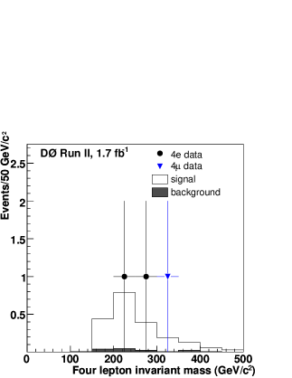
Figure 30: Distribution of four lepton invariant mass in data, expected signal, and expected background for the D0 $ZZ\rightarrow\ell\ell\ell\ell$ analysis [71].

Using a log-likelihood ratio test statistic of the yields and pseudo-experiments, the $p$-value is determined to be 4.3$\times$10^-8 which corresponds to a 5.3 $\sigma$ observed significance ($3.7\sigma$ expected). The measured cross section in the $ZZ\rightarrow\ell\ell\ell\ell$ channel is

$$\sigma(ZZ+X)=1.75^{+1.27}_{-0.86}~{}\mathrm{(stat.)}\pm 0.13~{}\mathrm{(syst.)}~{}\rm{pb}.$$

This result is combined with the results from an independent $ZZ\to\ell\ell\nu\nu$ search [72], and the previous $ZZ\rightarrow\ell\ell\ell\ell$ analysis [69] taking into account the systematic uncertainty correlations between subchannels and among analyses. The resulting $p$-value is 6.2$\times$10^-9, and the significance for observation of $ZZ$ production increases to $5.7\sigma$ ($4.8\sigma$ expected). This is the first observation of $ZZ$ production at a hadron collider. The combined cross section is

$$\sigma(ZZ+X)=1.60\pm 0.63~{}\mathrm{(stat.)}^{+0.16}_{-0.17}~{}\mathrm{(syst.)}~{}\rm{pb},$$

consistent with the SM expectation.

III.5.7 $WV$ ($V=W,Z$)

The production of vector boson pairs ($WW$, $WZ$, and $ZZ$) have been observed at the Tevatron in decay modes where both vector bosons decay leptonically. The semileptonic decay modes where one of the vector boson decay hadronically has larger branching fraction as compared to the fully leptonic modes but significantly larger backgrounds from jets produced in association with a $W$ boson. As a result, simple event counting above background cannot be used to observe dibosons in semileptonic decay at the Tevatron and advanced analysis techniques utilizing multivariate event classification are required to statistically separate signal from background. Analysis of the $\ell\nu jj$ final state provides an excellent testbed for such advanced techniques to extract small signals from large backgrounds in real hadron collision data that has great relevance to Higgs boson (e.g. $WH\rightarrow\ell\nu b\bar{b}$) and new physics searches in final states involving jets. In addition, semileptonic diboson decay can provide a more sensitive search for anomalous trilinear gauge couplings than fully leptonic decay modes since anomalous TGCs enhance production at high gauge boson momentum where the signal-to-background ratio improves.

The dijet mass resolution of the CDF and D0 detectors is not good enough to distinguish hadronically decaying $W$ bosons and $Z$ bosons. As a result, the search for diboson production in the $\ell\nu jj$ final state is a search for the sum of $WW$ and $WZ$ production. The experimental signature of the $WW+WZ$ signal in semileptonic decay is one isolated high $E_{T}$ charged lepton, large $E\kern-6.00006pt\raise 0.43057pt\hbox{/}_{T}$ from the neutrino produced in $W$ decay, and at least two high $E_{T}$ jets.

In principle, one could search for SM $WZ+ZZ$ production in the $jj\ell\ell$ channel. Large $Z$+jets backgrounds makes this a very difficult channel to observe the SM signal, although the use of $b$-tagging can improve the sensitivity. The use of the $b\bar{b}\ell\ell$ channel to search for associated Higgs boson production is described in Section V.2.2.

Both D0 and CDF have searched for $WW+WZ$ production and anomalous $WW\gamma$, $WWZ$ couplings in the $\ell\nu jj$ final state [73; 74; 75; 76]. In these analyses, $W+$jets is the dominant background. Other significant backgrounds include $Z$+jets, $t\bar{t}$, single top quark, and QCD multijet production. Backgrounds are suppressed by requiring a minimum $W$ transverse mass $M_{T}(W)$ in each event, which is the transverse mass of the charged lepton and $E\kern-6.00006pt\raise 0.43057pt\hbox{/}_{T}$ system.

The strategy for extracting the semileptonic $WW+WZ$ signal yield after basic event selection differs between the D0 and CDF analyses. In the D0 analysis [73], thirteen kinematic variables (e.g. dijet mass) demonstrating a sensitivity to distinguish signal and background are used as input to a Random Forest (RF) [77] multivariate event classifier using $\int{\cal L}~{}dt=1.1~{}\rm{fb}^{-1}$. Fig. 31 shows the RF output distribution after a fit to the $WV$ signal and $W+$jets background contributions. Fig. 32 shows the dijet mass distribution using the results of the RF output fit. The dominant systematic uncertainties arise from the modeling of the $W+$jets background and the jet energy scale. The probability for the background to fluctuate to give an excess as large as that observed in the data is $<5.4\times 10^{-6}$, corresponding to a 4.4$\sigma$ signal significance. This result is the first evidence for $WV$ production is lepton $+$ jets events at a hadron collider. The measured cross section is

$$\sigma(WV+X)=20.2\pm 4.5\rm{(stat.+syst.)}~{}\rm{pb}$$

consistent with the NLO SM cross section of $16.1\pm 0.9$ pb [64].

(a)
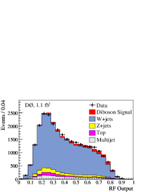
(b)

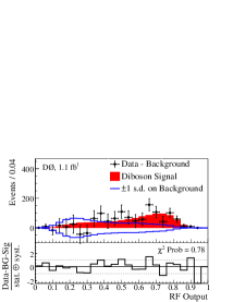
Figure 31: For the D0 analysis [73], (a) the RF output distribution from the combined $e\nu q\bar{q}$ and $\mu\nu q\bar{q}$ channels for data and simulated event predictions following the fit of simulation to data. (b) A comparison of the extracted signal (filled histogram) to background-subtracted data (points), along with the $\pm 1$ standard deviation (s.d.) systematic uncertainty on the background. The residual distance between the data points and the extracted signal, divided by the total uncertainty, is given at the bottom.

(a)
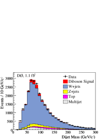
(b)

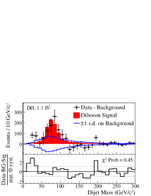
Figure 32: For the D0 analysis [73], (a) the dijet mass distribution from the combined $e\nu q\bar{q}$ and $\mu\nu q\bar{q}$ channels for data and simulated event predictions following the fit to the RF output. (b) A comparison of the extracted signal (filled histogram) to background-subtracted data (points), along with the $\pm 1$ standard deviation (s.d.) systematic uncertainty on the background.The residual distance between the data points and the extracted signal, divided by the total uncertainty, is given at the bottom.

In the CDF analysis [74], two different methods are used to extract the $WW+WZ$ signal from the data. In the first method (“dijet method”), the dijet invariant mass $M_{jj}$ is used to extract a signal peak from data corresponding to $\int{\cal L}~{}dt=3.9~{}\rm{fb}^{-1}$. The second method (“ME method”) takes advantage of more kinematic information in the event by constructing a discriminant based on calculations of the differential cross sections of the signal and background processes data corresponding to $\int{\cal L}~{}dt=2.7$ fb^-1. The ME method was discussed in Section III.5.4 where it was used in the $WW\rightarrow\ell\nu\ell\nu$ analysis and has been used in a number of different CDF and D0 analyses.

The normalization of the $Z$+jets background is based on the measured cross section [78]. The $t\bar{t}$ and single top background normalizations are from the NLO predicted cross sections [79; 80]. The efficiencies for the $Z$+jets, $t\bar{t}$, and single top backgrounds are estimated from simulation. The normalization of the multijet background is estimated by fitting the $E\kern-6.00006pt\raise 0.43057pt\hbox{/}_{T}$ spectrum in data to the sum of all contributing processes, where the multijet and $W$+jets normalizations float in the fit. In the final signal extractions from both methods, the multijet background is Gaussian constrained to the result of this $E\kern-6.00006pt\raise 0.43057pt\hbox{/}_{T}$ fit and the $W$+jets background is left unconstrained.

In the dijet method, the signal fraction in the data is estimated by performing a $\chi^{2}$ fit to the dijet invariant mass spectrum, separately for electron and muon events. Fig. 33 shows the dijet invariant mass distribution of data compared to the fitted signal and background contributions. The observed (expected) signal significance using the dijet method is 4.6$\sigma$ (4.9$\sigma$) for electrons and muons combined. The measured cross section is

$$\sigma(WV+X)=14.4\pm 3.1\rm{(stat.)}\pm 2.2\rm{(syst.)}~{}\rm{pb}$$

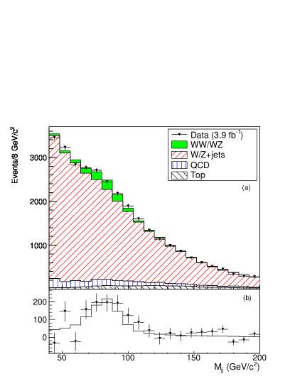
Figure 33: For the CDF analysis [74], the (a) dijet invariant mass distribution of reconstructed $W/Z\rightarrow jj$ candidates compared to the fitted signal and background components, and (b) corresponding background subtracted distribution.

In the ME method, the calculated event probabilities are combined into an event probability discriminant $EPD=P_{signal}/(P_{signal}+P_{background})$, where $P_{signal}=P_{WW}+P_{WZ}$ and $P_{background}=P_{W+jets}+P_{single\;top}$. Templates of the $EPD$ generated for all signal and background processes are used in a binned likelihood fit for the signal yield observed in the data, as shown in Fig. 34. Fig. 35 shows the dijet mass in bins of $EPD$, where it can be seen that the low $EPD$ bin contains very little signal as compared to background. Events with $EPD>0.25$ have a dijet mass peak close to the expected $W/Z$ mass, and the signal-to-background ratio improves with increasing $EPD$. The observed (expected) signal significance using the ME method is 5.4$\sigma$ (5.1$\sigma$) which represents the first observation of $WW+WZ$ production in the lepton + jets channel. The measured cross section using the ME method is

$$\sigma(WV+X)=17.7\pm 3.1({\rm stat.})\pm 2.4({\rm syst.})~{}\rm{pb}.$$

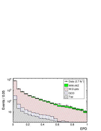
Figure 34: Observed $EPD$ distribution superimposed on distribution expected from simulated processes for the CDF analysis [74]

.

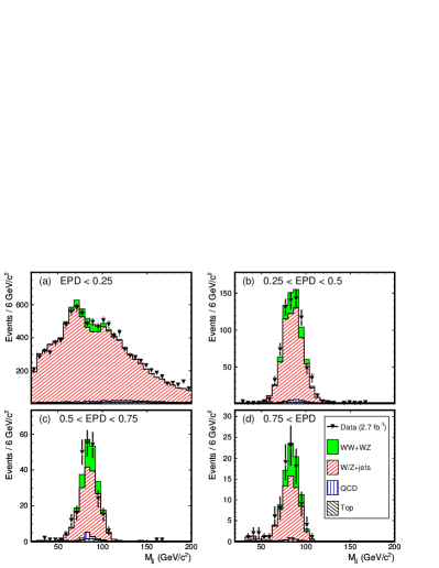
Figure 35: For the CDF analysis [74], $M_{jj}$ for events with (a) $EPD<0.25$, (b) $0.25<EPD<0.5$, (c) $0.5<EPD<0.75$, and (d) $EPD>0.75$.

In the $M_{jj}$ method the largest systematic uncertainties are due to the modeling of the EW and multijet shapes, about 8% and 6% respectively. In the ME method the uncertainty in the jet energy scale is the largest systematic uncertainty, at about 10%, which includes contributions both from the signal acceptance and from the shapes of the signal templates. In the $M_{jj}$ method this uncertainty is about 6%. The combined cross section for the dijet and ME methods, with consideration of statistical and systematic uncertainties, is

$$\sigma(WV+X)=16.0\pm 3.3({\rm stat.+syst.})~{}\rm{pb}.$$

Both of the CDF and D0 $WW+WZ$ cross section measurements are consistent with the SM NLO expectations. In [75], CDF searches for anomalous $WW\gamma$ and $WWZ$ couplings using the observed spectrum of the charged lepton $p_{T}$ from a $W$ decay and $\int{\cal L}~{}dt=0.35~{}\rm{fb}^{-1}$. Fig. 36 shows good consistency between the SM expectation for $W$ boson $p_{T}$ and the data which is used to constrain possible anomalous couplings. In order to increase the sensitivity to anomalous couplings, these data are combined with the photon $E_{T}$ spectrum from the $W\gamma$ analysis [46] described in Section III.5.2 that constrains possible anomalous $WW\gamma$ couplings. Tab. 17 summarizes the resulting anomalous coupling limits under the assumption of equal $WW\gamma$ and $WWZ$ couplings.

Figure 36: The $p_{T}^{W}$ distribution used for setting the anomalous TGC limits in the CDF analysis [75]. Shown are the SM expectation, data points, and one anomalous coupling scenario with $\lambda=\Delta\kappa=0.5$ and $\Lambda=1.5$ TeV.

	$\lambda$	$\Delta\kappa$
$\ell\nu jj$	(-0.28, 0.28)	(-0.50, 0.43)
$\ell\nu\gamma$ [46]	(-0.21, 0.19)	(-0.74, 0.73)
Combined	(-0.18, 0.17)	(-0.46, 0.39)

Table 17: Allowed anomalous coupling ranges for $\Lambda=1.5$ TeV at 95% CL, fixing the other coupling to the SM value and assuming equal $WW\gamma$ and $WWZ$ couplings for the CDF analysis [75].

The D0 search for anomalous couplings in the $\ell\nu jj$ channel [76] is based on the same data that was used to obtain the first evidence for semileptonic decays of $WW/WZ$ boson pairs in hadron collisions [73]. In contrast to the CDF analysis just described, the D0 analysis uses the dijet $p_{T}$ information to place limits on $WW\gamma/Z$ anomalous couplings. Fig. 37 shows the dijet $p_{T}$ distribution after a fit for the individual signal and background contributions. No excess at high dijet $p_{T}$ that would suggest that non-standard couplings are present is evident in the data. The one-dimensional 95% CL limits for the $WW\gamma/Z$ anomalous coupling parameters under separate assumptions of $SU(2)_{L}\otimes U(1)_{Y}$ symmetry and equal $WW\gamma$ and $WWZ$ couplings are shown in Tab. 18. The 2D limits under the assumption of $SU(2)_{L}\otimes U(1)_{Y}$ symmetry [6] is shown in Fig. 38 and for equal coupling assumption they are shown in Fig. 39.

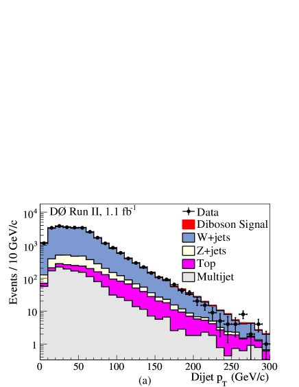
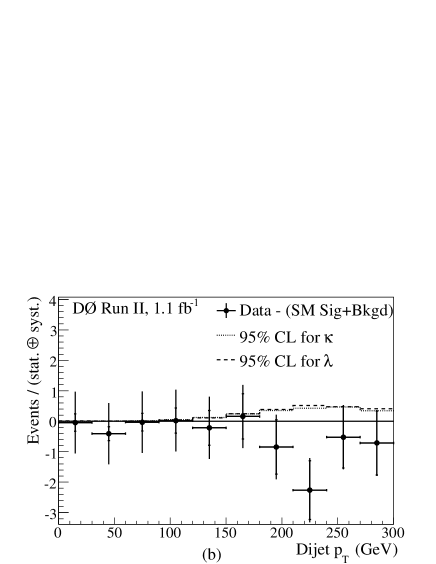
Figure 37: For the D0 analysis [76], the (a) dijet $p_{T}$ distribution of combined (electron+muon) channels for data and SM predictions following the fit of simulated events to data and (b) difference between data and simulation divided by the uncertainty (statistical and systematic) for the dijet $p_{T}$ distribution. Also shown are the simulated signals for anomalous couplings corresponding to the 95% CL limits for $\Delta\kappa$ and $\lambda$ in the LEP parametrization scenario. The full error bars on the data points reflect the total (statistical and systematic) uncertainty, with the ticks indicating the contribution due only to the statistical uncertainty.

68% CL	$\kappa_{\gamma}$	$\lambda=\lambda_{\gamma}=\lambda_{Z}$	$g_{1}^{Z}$
$SU(2)_{L}\otimes U(1)_{Y}$ symmetry	$\kappa_{\gamma}=1.07^{+0.26}_{-0.29}$	$\lambda=0.00^{+0.06}_{-0.06}$	$g_{1}^{Z}=1.04^{+0.09}_{-0.09}$
Equal couplings	$\kappa_{\gamma}=\kappa_{Z}=1.04^{+0.11}_{-0.11}$	$\lambda=0.00^{+0.06}_{-0.06}$
95% CL	$\Delta\kappa_{\gamma}$	$\lambda=\lambda_{\gamma}=\lambda_{Z}$	$\Delta{g_{1}^{Z}}$
$SU(2)_{L}\otimes U(1)_{Y}$ symmetry	-0.44 $<\Delta\kappa_{\gamma}<$ 0.55	-0.10 $<\lambda<$ 0.11	-0.12 $<\Delta g_{1}^{Z}<$ 0.20
Equal couplings	-0.16 $<\Delta\kappa<$ 0.23	-0.11 $<\lambda<$ 0.11

Table 18: The most probable values with total uncertainties (statistical and systematic) at 68% CL for $\kappa_{\gamma}$, $\lambda$, and $g_{1}^{Z}$ along with observed 95% CL one-parameter limits on $\Delta\kappa_{\gamma}$, $\lambda$, and $\Delta g_{1}^{Z}$ measured in 1.1 fb^-1 of $WW/WZ\rightarrow\ell\nu jj$ events with $\Lambda_{NP}=$ 2 TeV for the D0 analysis [76].

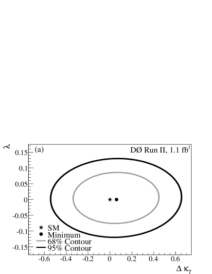
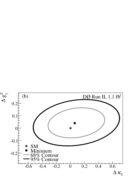
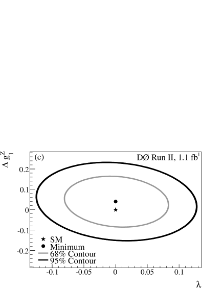
Figure 38: The 68% CL and 95% CL two-parameter limits on the $\gamma WW/ZWW$ coupling parameters $\Delta\kappa_{\gamma}$, $\lambda$, and $\Delta g_{1}^{Z}$, in the LEP parametrization scenario and $\Lambda_{NP}=$ 2 TeV for the D0 analysis [76]. The dots indicate the most probable values of anomalous couplings from the two-parameter combined (electron+muon) fit and the star markers denote the SM prediction.

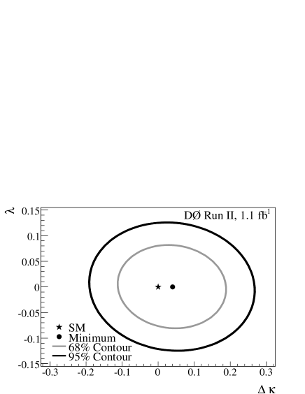
Figure 39: The 68% CL and 95% CL two-parameter limits on the $\gamma WW/ZWW$ coupling parameters $\Delta\kappa$ and $\lambda$, in the equal couplings scenario and $\Lambda_{NP}=$ 2 TeV for the D0 analysis [76]. The dot indicates the most probable values of anomalous couplings from the two-parameter combined (electron+muon) fit and the star marker denotes the SM prediction.

III.5.8 $VV$ ($V=W,Z$)

In Sections III.5.4-III.5.6, we summarized the observations of heavy vector boson pairs ($WW,WZ,ZZ$) when each boson decays to one or more charged leptons. In Section III.5.7, the measurements of a hadronically decaying heavy vector boson produced in association with a $W$ boson that decays to a charged lepton and a neutrino was described. Observing diboson production in semileptonic decay mode required sophisticated analysis techniques because of overwhelming $W+$jets in addition to the presence of a $WW+WZ$ signal. The approach of searching for diboson production in an more inclusive way can be taken a step further by dropping the requirement of a reconstructed charged lepton and instead looking at the $E\kern-6.00006pt\raise 0.43057pt\hbox{/}_{T}$ + jets final state. This approach includes an additional contribution from $Z\rightarrow\nu\nu$ over the $WW/WZ\rightarrow\ell\nu jj$ mode so that it measures $WW+WZ+ZZ$ production and allows for an event with a diboson decay to be accepted even if one or more charged leptons fail a selection cut. The experimental challenge is that this mode requires a tighter $E\kern-6.00006pt\raise 0.43057pt\hbox{/}_{T}$ cut as compared to $WW/WZ\rightarrow\ell\nu jj$ and a better overall understanding of high reconstructed $E\kern-6.00006pt\raise 0.43057pt\hbox{/}_{T}$ tails from low true $E\kern-6.00006pt\raise 0.43057pt\hbox{/}_{T}$ events with large cross section like QCD multijets.

The CDF Collaboration uses $\int{\cal L}~{}dt=3.5~{}\rm{fb}^{-1}$ to search for the production of heavy vector boson pairs ($VV$, $V$=$W,Z$) where one boson decays to a dijet final state [81]. The most significant backgrounds to the diboson signal are $W$$(\ell\nu)$+jets, $Z$$(\nu\nu)$+jets, and QCD multijet production. Other less significant backgrounds include $Z$$(\ell\ell)$+jets, $t\bar{t}$, and single $t$-quark production. The majority of events are collected using an inclusive $E\kern-6.00006pt\raise 0.43057pt\hbox{/}_{T}$ trigger which requires $\mbox{$E\kern-6.00006pt\raise 0.43057pt\hbox{/}_{T}$}>45$ GeV. In the offline selection, events are required to have $\mbox{$E\kern-6.00006pt\raise 0.43057pt\hbox{/}_{T}$}>60$ GeV and exactly two reconstructed jets with $E_{T}>25$ GeV and $|\eta|<2.0$.

The shape and normalization of the multijet background are determined from the data. A tracking-based missing momentum vector, $\mathbin{\vec{p\mkern-8.0mu/}_{T}}$, analogous to the calorimeter-based $\mathbin{\vec{E\mkern-11.0mu/}_{T}}$, is constructed from the vector sum of the transverse momenta of particles measured in the tracking system, and is largely uncorrelated to $\mathbin{\vec{E\mkern-11.0mu/}_{T}}$ for events where jets are misreconstructed. In the absence of $E\kern-6.00006pt\raise 0.43057pt\hbox{/}_{T}$ arising from mismeasurement in the calorimeter, the $\mathbin{\vec{E\mkern-11.0mu/}_{T}}$ and $\mathbin{\vec{p\mkern-8.0mu/}_{T}}$ will be aligned in most events. At large values of $\Delta\phi$(${\mathbin{\vec{E\mkern-11.0mu/}_{T}}},{\mathbin{\vec{p\mkern-8.0mu/}_{T}}}$), multijets are expected to be the dominant component of the data. The dijet mass shape and normalization for the multijet background that remains after the event selection is determined by selecting events with $\Delta\phi$(${\mathbin{\vec{E\mkern-11.0mu/}_{T}}},{\mathbin{\vec{p\mkern-8.0mu/}_{T}}}$)$>$1.0 and subtracting out the non-multijet backgrounds. The normalization is scaled up to account for the multijet background contamination in the region $\Delta\phi$(${\mathbin{\vec{E\mkern-11.0mu/}_{T}}},{\mathbin{\vec{p\mkern-8.0mu/}_{T}}}$)$<$1.0. The shape of the multijet background is fit to an exponential in $M_{jj}$ to derive a dijet mass template for use in the $M_{jj}$ unbinned extended likelihood fit performed to extract the diboson signal. The distribution of $\Delta\phi_{\mbox{$E\kern-4.20004pt\raise 0.3014pt\hbox{/}_{T}$}}^{jet}$ observed in the data is in good agreement with the expectations as shown in Fig. 40, giving confidence in the validity of the multijet background model.

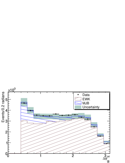
Figure 40: Data compared with the sum of the predicted EW and multijet backgrounds for the $\Delta\phi^{jet}_{\mbox{$E\kern-4.20004pt\raise 0.3014pt\hbox{/}_{T}$}}$ variable in the CDF analysis [81]. The band represents the total systematic uncertainty on the background. The measured signal is included here in the EW contribution.

Three $M_{jj}$ template distributions are used in the fit: the first is $V$+jets and $t$-quark production and is taken from Monte Carlo simulation; the second is the multijet template, where the slope and normalization are Gaussian constrained to their previously measured values; the third template describes the signal. The signal shape is comprised of the $WW,~{}WZ$, and $ZZ$ distributions obtained from a Gaussian + polynomial fit to the signal Monte Carlo simulation where the mean and the width of the Gaussian distribution are linearly dependent on the jet energy scale (JES). The uncertainty associated with the JES is the dominant source of systematic uncertainty of the diboson cross section measurement.

Fig. 41 shows the fit result and a comparison between the expected signal and data after background subtraction. The signal significance is reported to be greater than 5.3$\sigma$ from the background-only hypothesis. This represents the first observation in hadronic collisions of the production of weak gauge boson pairs where one boson decays to a dijet final state. The measured cross section is

$$\sigma(WW+WZ+ZZ+X)$$

$${}=18.0~{}\pm~{}2.8\mathrm{(stat.)}~{}\pm~{}2.4\mathrm{(syst.)}~{}\pm~{}1.1\mathrm{(lumi.)}~{}\rm{pb},$$

consistent with the SM NLO prediction of 16.8 $\pm$ 0.5 pb [64].

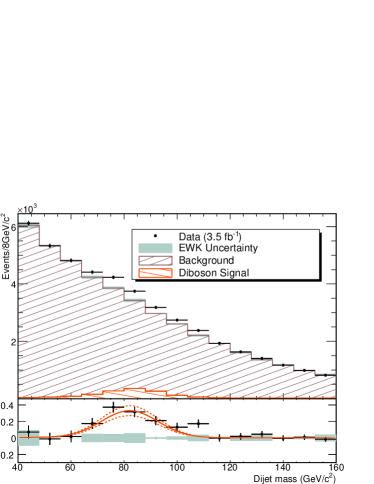
Figure 41: Top: Comparison between data and fitted background only. The measured signal is shown unstacked. The band represents the systematic uncertainty due to the shape of EW background as described in [81]. Bottom: Comparison of the diboson signal (solid line) with the background-subtracted data (points). The dashed lines represent the $\pm 1\sigma$ statistical variations on the extracted signal. The gray band represents the systematic uncertainty due the EW shape.

III.5.9 Cross Section and Anomalous TGC Summary

A summary of the diboson production cross sections at the Tevatron with comparisons to the theory expectations can be found in Tab. 19 and Fig. 42. A summary of limits on anomalous charged and neutral TGCs at the Tevatron can be found in Tab. 20 and Tab. 21, respectively.

The experimental progress on diboson physics during Run II at the Fermilab Tevatron has been truly remarkable. This includes the first observation of $WZ$ production and the first observation at a hadron collider of $ZZ$ production and of weak gauge boson pair production in semileptonic decay. The associated diboson cross section measurements (many of which are significantly improved from Run I) and detailed studies of their kinematic properties provide stringent tests standard electroweak theory and constraints on possible new physics coupling to the EW gauge bosons.

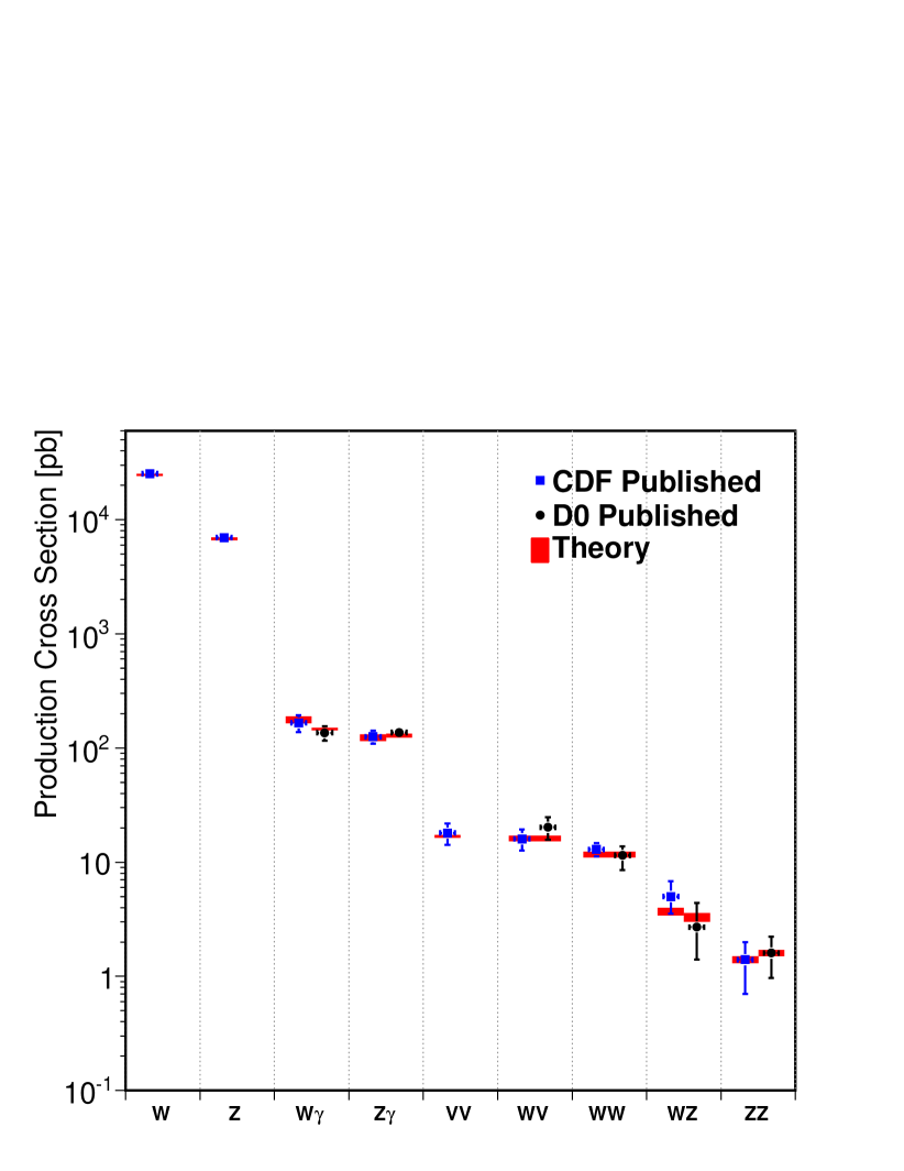
Figure 42: A graphical summary of EW gauge boson cross section measurements and theory expectations during Run II and the Fermilab Tevatron.

Process	Channel	$\int{\cal L}\ dt$ (fb-1)	Cross section (pb)		Expt.
			Theory	Measured	Reference
$p\bar{p}\rightarrow W\gamma+X\rightarrow\ell\nu\gamma+X$
($E_{T}^{\gamma}>7$ GeV, $\Delta R_{\ell,\gamma}>0.7$)	$\ell\nu\gamma$	$\sim 0.2$	$19.3\pm 1.4$ [43]	$18.1\pm 3.1~{}{\rm(stat.+syst.)}$	CDF [46]
($E_{T}^{\gamma}>8$ GeV, $\Delta R_{\ell,\gamma}>0.7$)	$\ell\nu\gamma$	$\sim 0.2$	$16.0\pm 0.4$ [43]	$14.8\pm 1.9~{}{\rm(stat.+syst.)}\pm 1.0~{}{\rm(lumi.)}$	D0 [47]
$p\bar{p}\rightarrow Z\gamma+X\rightarrow\ell\ell\gamma+X$
($E_{T}^{\gamma}>7$ GeV, $\Delta R_{\ell,\gamma}>0.7$,
$M_{\ell\ell}>40$ GeV/$c^{2}$)	$\ell\ell\gamma$	$\sim 0.2$	$4.5\pm 0.3$ [57]	$4.6\pm 0.6~{}{\rm(stat.+syst.)}$	CDF [46]
($E_{T}^{\gamma}>7$ GeV, $\Delta R_{\ell,\gamma}>0.7$,
$M_{\ell\ell}>30$ GeV/$c^{2}$)	$\ell\ell\gamma$	$\sim 1.1$	$4.7\pm 0.2$ [57]	$5.0\pm 0.3~{}{\rm(stat.+syst.)}\pm 0.3~{}{\rm(lumi.)}$	D0 [56]
$p\bar{p}\rightarrow Z\gamma+X\rightarrow\nu\nu\gamma+X$
($E_{T}^{\gamma}>90$ GeV)	$\nu\nu\gamma$	$3.6$	$0.039\pm 0.04$ [57]	$0.032\pm 0.09~{}{\rm(stat.+syst.)}\pm 0.02~{}{\rm(lumi.)}$	D0 [58]
$p\bar{p}\rightarrow WW+X$	$\ell\nu\ell\nu$	3.6	$11.7\pm 0.7$ [64]	$12.9\pm 0.9~{}{\rm(stat.)}^{+1.6}_{-1.4}~{}{\rm(syst.)}$	CDF [62]
	$\ell\nu\ell\nu$	$\sim 1.1$		$11.5\pm 2.1~{}{\rm(stat.+syst.)}\pm 0.7~{}{\rm(lumi.)}$	D0 [63]
$p\bar{p}\rightarrow WZ+X$	$\ell\ell\ell\nu$	1.1	$3.7\pm 0.3$ [64]	$5.0^{+1.8}_{-1.4}~{}{\rm(stat.)}\pm 0.4~{}{\rm(syst.)}$	CDF [65]
	$\ell\ell\ell\nu$	1.0		$2.7^{+1.7}_{-1.3}~{}{\rm(stat.+syst.)}$	D0 [67]
$p\bar{p}\rightarrow ZZ+X$	$\ell\ell\ell\ell$, $\ell\ell\nu\nu$	1.9	$1.4\pm 0.1$ [64]	$1.4^{+0.7}_{-0.6}~{}{\rm(stat.+syst.)}$	CDF [70]
	$\ell\ell\ell\ell$, $\ell\ell\nu\nu$	1.7		$1.6\pm 0.6~{}{\rm(stat.)}\pm 0.2~{}{\rm(syst.)}$	D0 [71]
$p\bar{p}\rightarrow WV+X$ ($V\rightarrow W,Z$)	$\ell\nu qq$	2.7	$16.1\pm 0.9$ [64]	$16.0\pm 3.3{\rm(stat.+syst.)}$	CDF [74]
	$\ell\nu qq$	1.1		$20.2\pm 4.5{\rm(stat.+syst.)}$	D0 [73]
$p\bar{p}\rightarrow VV+X$ ($V\rightarrow W,Z$)	$\ell\nu qq,\nu\nu qq$	3.5	$16.8\pm 0.5$ [64]	$18.0\pm 2.8{\rm(stat.)}\pm 2.4{\rm(syst.)}\pm 1.1{\rm(lumi.)}$	CDF [81]

Table 19: A tabular summary of EW gauge boson cross section measurements and theory expectations during Run II and the Fermilab Tevatron.

Mode	TGC(s)	$\int{\cal L}\ dt$	$\Lambda$	95% CL Limits (model constraints in parentheses)					Expt.
		(fb-1)	(TeV)	$\lambda_{\gamma}$	$\Delta\kappa_{\gamma}$	$\lambda_{Z}$	$\Delta g_{1}^{Z}$	$\Delta\kappa_{Z}$	Ref.
$\ell\nu\gamma$	$WW\gamma$	$\sim 0.7$	2.0	$-0.12,0.13$	$-0.51,0.51$	$-$	$-$	$-$	D0 [48]
$\ell\nu\ell\nu$	$WW(\gamma,Z)$	3.6	1.5	$-0.16,0.16$	$-0.63,0.72$	$\lambda_{\gamma}$	$-0.24,0.34$	$\Delta g^{Z}_{1}-\Delta\kappa_{\gamma}\tan^{2}\theta_{W}$	CDF
			2.0	$-0.14,0.15$	$-0.57,0.65$	$\lambda_{\gamma}$	$-0.22,0.30$	$\Delta g^{Z}_{1}-\Delta\kappa_{\gamma}\tan^{2}\theta_{W}$	CDF
		$\sim 1.1$	2.0	$-0.14,0.18$	$-0.54,0.83$	$\lambda_{\gamma}$	$-0.14,0.30$	$\Delta g^{Z}_{1}-\Delta\kappa_{\gamma}\tan^{2}\theta_{W}$	D0 [63]
			2.0	$-0.14,0.18$	$-0.12,0.35$	$\lambda_{\gamma}$	$0$	$\Delta\kappa_{\gamma}$	D0 [63]
$\ell\ell\ell\nu$	$WWZ$	$\sim 1.0$	1.5	$-$	$-$	$-0.18,0.22$	$-0.15,0.35$	$-0.14,0.31$
								($\Delta\kappa_{Z}=\Delta g_{1}^{Z}$)	D0 [67]
			2.0	$-$	$-$	$-0.17,0.21$	$-0.14,0.34$	$-0.12,0.29$
								($\Delta\kappa_{Z}=\Delta g_{1}^{Z}$)	D0 [67]
$\ell\nu qq,\ell\nu\gamma$	$WW(\gamma,Z)$	0.4	1.5	$-0.18,0.17$	$-0.46,0.39$	$\lambda_{\gamma}$	$0$	$\Delta\kappa_{\gamma}$	CDF [75]
		1.1	2.0	$-0.10,0.11$	$-0.44,0.55$	$\lambda_{\gamma}$	$-0.12,0.20$	$\Delta g^{Z}_{1}-\Delta\kappa_{\gamma}\tan^{2}\theta_{W}$	D0 [76]
				$-0.11,0.11$	$-0.16,0.23$	$\lambda_{\gamma}$	0	$\Delta\kappa_{\gamma}$	D0 [76]
$\ell\nu\gamma$,$\ell\nu\ell\nu$,$\ell\ell\ell\nu$,$\ell\nu qq$	$WW(\gamma,Z)$	$\sim$1.0	2.0	$-0.08,0.08$	$-0.29,0.38$	$\lambda_{\gamma}$	$-0.07,0.16$	$\Delta g^{Z}_{1}-\Delta\kappa_{\gamma}\tan^{2}\theta_{W}$	D0 [82]
				$-0.08,0.08$	$-0.11,0.18$	$\lambda_{\gamma}$	0	$\Delta\kappa_{\gamma}$	D0 [82]

Table 20: A summary of anomalous charged TGC limits for different diboson processes and decay channels measured during Run II and the Fermilab Tevatron.

Mode	TGC(s)	$\int{\cal L}\ dt$	$\Lambda$	95% CL Limits				Expt.
		(fb-1)	(TeV)					Ref.
$\ell\ell\ell\ell$	$ZZZ,ZZ\gamma$	1.0	1.2	$-0.28<f_{40}^{\gamma}<0.28$	$-0.26<f_{40}^{\gamma}<0.26$	$-0.31<f_{50}^{Z}<0.29$	$-0.30<f_{50}^{Z}<0.28$	D0 [69]
$\ell\ell\gamma,\nu\nu\gamma$	$Z\gamma\gamma,ZZ\gamma$	1.0, 3.6	1.5	$|h_{30}^{\gamma}|<0.033$	$|h_{40}^{\gamma}|<0.0017$	$|h_{30}^{Z}|<0.033$	$|h_{40}^{Z}|<0.0017$	D0 [58]

Table 21: A summary of anomalous neutral TGC limits for different diboson processes and decay channels measured during Run II and the Fermilab Tevatron.

IV TOP QUARK

IV.1 Top Quark Mass

As discussed in section V.1, constraints on the Higgs boson mass from fits to data assuming the SM are limited by the experimental precision of the $W$ boson and top quark masses. Measurements of the top quark mass thus have direct implications for the SM, and these measurements are a central component of the programs for both CDF and D0. As evidenced from Fig. 3, constraints on the Higgs mass are limited more by the uncertainty in the $W$ boson mass than by the uncertainty in the top-quark mass, which reflects the tremendous progress than has been made on the top-quark mass measurement in Run II. In fact, the top-quark mass is now the most accurately known quark mass (as a percentage of its value), surpassing even its $SU(2)_{\rm L}$ partner the $b$ quark, whose mass is known to about 2.6% ($\bar{m}_{b}(\bar{m}_{b})=4.24\pm 0.11\ {\rm GeV/c}^{2}$) [83].

The top-quark mass measured at the Tevatron corresponds closely to the pole mass. The pole mass is the mass the quark would have in the absence of confinement. Although the top quark decays on a time scale less than the time scale associated with confinement ($\Lambda_{QCD}^{-1}$), the top-quark pole mass is nevertheless affected by confinement [84]. The ambiguity in the top-quark pole mass is of order $\Lambda_{QCD}\approx 200$ MeV, which is considerably less than the present uncertainty. A more precise definition of mass will be needed if one attempts to measure the mass to an accuracy much less than 1 ${\rm GeV/c}^{2}$.

Both CDF and D0 have made measurements of the top quark mass in a variety of final states and using different methods. The general procedure is to select events consistent with $t\overline{t}$ production in either the dilepton or lepton plus jets final state. In the SM, top quarks decay via $t\to Wb$ with a branching fraction of essentially 100%. The dilepton final state is that in which both $W$ bosons from the $t\overline{t}$ pair decay to leptons, and the lepton+jets final state is that in which one $W$ decays to leptons and the other to quarks. Measurements of the mass have also been made in the all jets final state in which both $W$s decay to quarks, although this offers less precision because of significantly higher backgrounds.

An initial selection of candidate dilepton events is made, typically requiring two high $p_{T}$ charged leptons, significant $E\kern-6.00006pt\raise 0.43057pt\hbox{/}_{T}$ attributed to neutrinos, and at least two jets. Typical thresholds for the lepton and jet transverse momenta range between 15 ${\rm GeV/c}$ and 20 ${\rm GeV/c}$. The $E\kern-6.00006pt\raise 0.43057pt\hbox{/}_{T}$ is attributed to the two neutrinos from $t\overline{t}$ decay, and the thresholds are higher, ranging between 35 GeV and 50 GeV depending on topology. The initial selection of lepton+jets candidate events requires a single charged lepton, $E\kern-6.00006pt\raise 0.43057pt\hbox{/}_{T}$ and at least three (and often four) jets. The lepton and jet thresholds are similar to the dilepton final state, but the $E\kern-6.00006pt\raise 0.43057pt\hbox{/}_{T}$ threshold is typically relaxed giving requirements ranging from $\mbox{$E\kern-6.00006pt\raise 0.43057pt\hbox{/}_{T}$}>15$ GeV to $\mbox{$E\kern-6.00006pt\raise 0.43057pt\hbox{/}_{T}$}>20$ GeV. Because the lepton+jets events have significant background from $W$+jet events, an additional requirement that one or more of the jets is consistent with $B$ hadron production ($b$-tagged) is often made. The typical tagging efficiency is 50%/jet with light quark misidentification rates of roughly 1%. The probability to misidentify a charm quark induced jet as being consistent with $B$ hadron production is roughly 15%. Actual values vary somewhat depending on the $b$–tagging algorithm used. The values also depend on the signal-to-background requirements of the specific analysis which allow more or less restrictive tagging requirements. These loose initial selections have minimal top quark mass bias and form the basis for further analysis.

Typical signal and background estimates are given in Tab. 22 for various channels. In the selections, trade-offs are made between signal acceptance and purity. In particular, the requirement that an event have one or more jets consistent with being initiated by $b$-quarks considerably improves the signal purity.

	$\int{\cal L}~{}dt$	Expected	Estimated	Observed	$b$-tag	Expt.
Channel	(fb-1)	Signal Yield	Total Yield	Yield	Required?	Ref.
$\ell\ell$	2	$43.8\pm 4.4$	$215.8\pm 21.9$	246	$\equiv 0$	CDF[85]
		$78.0\pm 6.2$	$97.5\pm 7.2$	98	$\geq 1$
$\ell\ell$, $e\mu$	1	$36.7\pm 2.4$	$44.5\pm 2.7$	39	no	D0[86]
$\ell\ell$, $ee$		$11.5\pm 1.4$	$14.8\pm 1.5$	17
$\ell\ell$, $\mu\mu$		$8.3\pm 0.5$	$13.7\pm 0.7$	13
$\ell\ell$, $e$+track		$9.4\pm 0.1$	$10.3\pm 0.2$	8	$\geq 1$
$\ell\ell$, $\mu$+track		$4.6\pm 0.1$	$5.5\pm 0.1$	6
$\ell+\mathrm{jets}$	1.9	$183\pm 25$	$247\pm 29$	284	$=1$	CDF[87]
		$69\pm 11$	$75\pm 11$	87	$\geq 2$
$\ell+\mathrm{jets}$	1	$162\pm 11$	$57.2\pm 4.2$(est)	200	$\geq 1$	D0[88]

Table 22: Signal and background yields for preselected $t\overline{t}$ samples from a subset of the published results. The purity varies considerably depending on the final state and whether or not $b$-tagged jets are required.

After the initial selections, various methods are used to determine the top mass. Among these are: (1) template methods in which data are fit to the predicted signal plus background distribution for a variable that is sensitive to the top mass, (2) ME methods similar to those discussed in Sec. III.5.4 in which $t\overline{t}$ event kinematics determined by matrix element calculations are convoluted with detector resolution functions to predict measured kinematic distributions as a function of the top mass used in the matrix element calculations, and (3) other weighting methods in which missing information is supplied by trying possible reconstructed jet and true $t\overline{t}$ decay parton assignments and computing a probability for the particular assignment as a function of top mass. The ME and various weighting methods compute event-by-event likelihoods as a function of top mass, and then compute the total likelihood for a data set as the products of the event likelihoods. Combinations of these methods are also used.

For lepton+jets events, the momenta of the four jets and the lepton are fully measured, and the neutrino momentum in the plane transverse to the beam is inferred from the event $E\kern-6.00006pt\raise 0.43057pt\hbox{/}_{T}$. This gives seventeen measured values. Two constraints are available. The first is that the invariant mass of one pair of reconstructed jets should be consistent with that of the $W$ boson, and the second is that the reconstructed mass of the two top quarks should be consistent with each other. This information allows a one degree-of-freedom fit to be performed in which the top mass is a free parameter. The resulting event top mass values are not simply averaged to determine the mass, but provide an input variable to the various methods described above. The fit $\chi^{2}$ can also be used to determine (or weight) the most likely parton-jet assignment in an event. Complications to this fit arise from the presence of intrinsic transverse momentum of the $t\overline{t}$ system $p_{T}^{t\overline{t}}$ and from final state gluon radiation giving rise to additional jets. The $p_{T}^{t\overline{t}}$ can be incorporated by adding an additional variable for the unknown transverse momentum $\vec{X}$ to the fit and constraining it using a priori estimates of the spectrum. The impact of final state radiation can be controlled by requiring exactly four reconstructed (good) jets in the event.

For dilepton events, the number of measurements minus the number of constraints does not give enough information to fully determine the final state kinematics, and one assumption must be made. A variety of methods are used including ME weighting and neutrino weighting. The ME weighting method [89; 90; 91] is related to the general ME method described below (and also used for $\ell$+jets analyses). The neutrino weighting method [92; 93] is unique to dilepton events. In this method, an event weight is defined as a function of hypothesized top quark mass $M_{t}$ using a comparison of the measured $\vec{\mbox{$E\kern-6.00006pt\raise 0.43057pt\hbox{/}_{T}$}}$ to $\vec{\mbox{$E\kern-6.00006pt\raise 0.43057pt\hbox{/}_{T}$}}_{i}$ values predicted for a set of possible neutrino pseudorapidity values $\eta^{(1)}_{i},\eta^{(2)}_{i}$. Large weights correspond to situations in which the measured and predicted $\vec{\mbox{$E\kern-6.00006pt\raise 0.43057pt\hbox{/}_{T}$}}$ are similar and thus give a probability for different $\eta$ values for the neutrinos in each event.

The use of the ME approach has become widespread, especially for $\ell$+jets final states. It is used either as the final analysis variable used to determine the measured mass or to provide information used in joint likelihoods for determining the top mass. In this approach, the probability that the the jet momenta, lepton momentum and missing transverse energy observed in a given event, assuming it arises from $t\overline{t}$ production and decay, is computed by[88]

$$P_{t\overline{t}}=\frac{1}{N}\int\sum d\sigma(y;M_{t})\,dq1\,dq2\,f(q_{1})\,f(q_{2})\,W(y,x)$$

in which $d\sigma$ is the differential cross section for production of the final state partons in (momentum) configuration $y$ for a given $M_{t}$, $f(q_{1})$ and $f(q_{2})$ are the parton density functions for the proton and antiproton, $W(y,x)$ is the transfer function for computing the probability that a partonic final state $y$ gives the observed reconstructed final state $x$ and $1/N$ is a normalization factor equal to the expected observed cross section for a given $M_{t}$. For each event this probability, and the corresponding probability computed assuming the event is a background event, $P_{bkg}(x)$, are combined to give an event probability as a function of top mass

$$P(x;M_{t})=A(x)(fP_{t\overline{t}}(x;M_{t})+(1-f)P_{bkg}(x))$$

in which $A(x)$ is a normalization factor incorporating acceptance and efficiency effects and $f$ is the fraction of $t\overline{t}$ events in the total sample. The overall normalization of $P$ is forced to unity so that it can be used as a probability density. The event probability is then used either as input to additional likelihoods or the joint likelihood for the entire sample is formed as the product of the event probabilities and minimized as a function of $M_{t}$.

The methods used in early Run II top mass measurements had systematic uncertainty from the energy calibration of reconstructed jets which, if unmodified, would have quickly surpassed the statistical uncertainty. A method was developed to incorporate an in situ calibration scale factor as a second fit parameter when determining the top mass. As an example, the ME method event probability definition was modified to the form now in general use. This form is

$$P(x;M_{t},k_{jes})=A(x)$$

$${}\times\left[fP_{t\overline{t}}(x;M_{t},k_{jes})+(1-f)P_{bkg}(x;k_{jes})\right]$$

in which $k_{jes}$ is a scale factor applied to all jet energies. In this form the transfer functions also become dependent on the calibration, $W(y,x,k_{jes})$. The negative log likelihood minimized to determine the top mass thus becomes a function of two variables, $m_{top}$ and $k_{jets}$, both of which are varied during the minimization. As an example, Fig. 43 shows the 2D contour in the $\Delta_{jes}\equiv k_{jes}-1$ versus $m_{top}$ plane from the $M_{t}$ measurement using the $\ell\ell$ and $\ell+\mathrm{jets}$ final states simultaneously. [94].

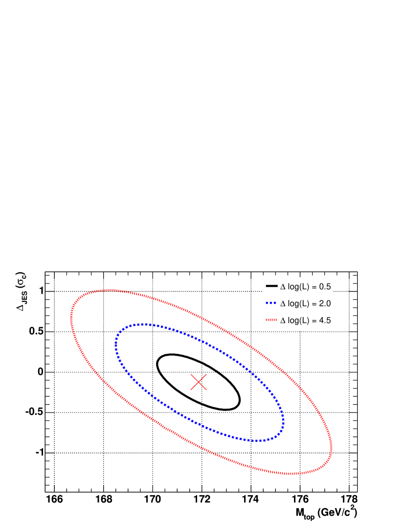
Figure 43: Contours of constant -log(L) in the $\Delta_{jes}\equiv k_{jes}-1$ versus $M_{t}$ plane[94]. A perfect a priori jet energy calibration used as input to this analysis would result in $k_{jes}=1$ corresponding to $\Delta_{jes}=0$.

Systematic uncertainties in top mass measurements arise from both experimental sources and theory. Although the contribution from calibration uncertainties has been significantly reduced as described in the previous paragraph, the dominant contributions to the systematic uncertainty from experimental sources are the absolute reconstructed jet energy calibration and the relative calibrations of jets initiated by $b$-quarks and those from light quarks ($u,\ d,\ s$). Of these, the uncertainty from the jet calibrations dominates the experimental uncertainties. Uncertainties arising from theory include production model as assessed by comparing event generators and fragmentation. The production model uncertainty becomes the dominant theory uncertainty when various measurements are combined.

Tab. 23 and Fig. 44 give a summary of the published top mass results and a comparison with the 2008 Particle Data Group (PDG)[37] average. When multiple results from one experiment using the same method and final state were available, only the highest integrated luminosity measurement is reported. The result shown in Tab. 23 with highest integrated luminosity used a $\int{\cal L}~{}dt\ =2.9\,\mathrm{fb}^{-1}$ data sample. The Tevatron experiments have now reported preliminary results using up to 4 fb^-1, and these results have been included in a world average combination by the Tevatron Electroweak Working Group, with the most recent such combination [95] giving

$$M_{t}=173.1\pm 0.6\ \mathrm{(stat.)}\pm 1.1\mathrm{(syst.)}\ {\rm GeV/c}^{2}.$$

For this combination, which does include preliminary results, the systematic uncertainty is significantly larger than the statistical uncertainty. The dominant components of the systematic uncertainty arise from uncertainty on the in situ jet energy calibration, uncertainty related to the $t\overline{t}$ production and decay model and uncertainty arising for color recombination. These contribute $0.48\ {\rm GeV/c}^{2}$, $0.49\ {\rm GeV/c}^{2}$ and $0.41\ {\rm GeV/c}^{2}$ to the uncertainty, respectively.

An alternative method of measuring the top quark mass makes use of the dependence of the production cross section on the mass. The top quark $\overline{MS}$ mass may be extracted directly from such a method [96].

By the end of the Tevatron running, the experiments expect to increase the data set by at least a factor of four compared to the published results and at least a factor of two for the data sets used in the combination. Thus, the statistical precision can be improved, but the systematic uncertainties will also need to be improved if the full statistical power of the final data set is to be realized.

	$\int{\cal L}~{}dt$	Analysis		Main Systematic Uncertainty		Expt.
Channel	(fb-1)	Method	$M_{t}$ (${\rm GeV/c}^{2}$)	Source	Value	Ref.
					(GeV/c2)
$\ell\ell+(\ell+\mathrm{jets})$	1.9		$171.9\pm 1.7\mathrm{(stat+JES)}\pm 1.1\mathrm{(syst)}$			CDF[94]
$\ell\ell$	2.9	$\phi$ WT	$165.5^{+3.4}_{-3.3}\mathrm{(stat)}\pm 3.1\mathrm{(syst)}$	jet calibration	$2.2$	CDF[97]
	2	Matrix	$171.2\pm 2.7\mathrm{(stat)}\pm 2.9\mathrm{(syst)}$	jet calibration	$2.5$	CDF[85]
	1.2	Template+$M_{t}$	$170.7^{4.2}_{-3.9}\mathrm{(stat)}\pm 2.6\mathrm{(syst)}\pm 2.4\mathrm{(theo)}$	jet calibration	$1.8?$	CDF[98]
	1	Matrix	$164.5\pm 3.9\mathrm{(stat)}\pm 3.9\mathrm{(syst)}$	jet calibration	$3.5$	CDF[99]
	1	Matrix+$\nu$WT	$174.7\pm 4.4\mathrm{(stat)}\pm 2.0\mathrm{(syst)}$	jet calibration	$1.2$	D0[86]
$\ell+\mathrm{jets}$	1.9	Matrix	$172.7\pm 1.8\mathrm{(stat)}\pm 1.2\mathrm{(syst)}$	generator, jet calib	$0.6,\ 0.5$	CDF[87]
	1	Matrix	$171.5\pm 1.8\mathrm{(stat+JES)}\pm 1.1\mathrm{(syst)}$	$b/u,d,s$, frag.	$0.83$	D0[88]
	0.7	Decay Length	$180.7^{+15.5}_{-13.4}\mathrm{(stat)}\pm 8.6\mathrm{(syst)}$	Bkg. shape	$6.8$	CDF[100]
	0.4	Ideogram	$173.7\pm 4.4\mathrm{(stat+JES)}\pm 2.1\mathrm{(syst)}$	$b/u,d,s$ calib.	$1.7$	D0[101]
	0.3	Template+DLL	$173.5^{+3.7}_{-3.6}\mathrm{(stat+JES)}\pm 1.3\mathrm{(syst)}$	signal model	$1.1$	CDF[102]
All jets	1	Lineshape	$174.0\pm 2.2\mathrm{(stat)}\pm 4.8\mathrm{(syst)}$	jet calibration	$4.5$	CDF[103]
	1.0	Matrix	$171.1\pm 3.7\mathrm{(stat+JES)}\pm 2.1\mathrm{(syst)}$	parton shower, jet calib	$0.6,\ 0.5$	CDF[104]
$\mbox{$E\kern-6.00006pt\raise 0.43057pt\hbox{/}_{T}$}+\mathrm{jets}$	0.3	Spectra	$172.3^{10.8}_{-9.6}\mathrm{(stat)}\pm 10.8\mathrm{(syst)}$	jet calibration	$9.6$	CDF[105]
Tevatron (incl. prel.)			$173.1\pm 0.6\mathrm{(stat)}\pm 1.1\mathrm{(syst)}$			CDF+D0[95]
Particle Data Group 2008			$171.2\pm 2.1$			PDG[37]

Table 23: Summary of published Run II top quark mass measurements. Additional preliminary results using up to $\int{\cal L}~{}dt=4$ fb^-1 have been reported by both CDF and D0. The Particle Data Group average includes only some of these results, and the Tevatron average is based on a subset of the results in this table and additional preliminary results.

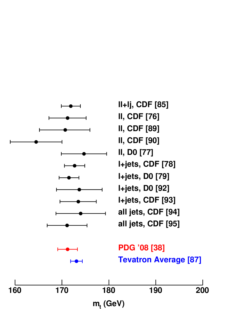
Figure 44: Published top mass measurements. For a given experiment and final state, the results from different methods have a significant correlation. Also shown are the most recent Tevatron combination[95] and the PDG world average. Both of these include a subset of the measurements listed in this table.

IV.2 $W$ Helicity from Top Quark Decays

In the SM, top quarks decay with a V-A interaction through the process $t\to W^{+}b$ with $B(t\to W+b)\approx 1$. The SM predicts a fraction $f_{0}=0.697\pm 0.012$ of top quark decays give a longitudinally polarized $W$ and a fraction $f_{+}=3.6\times 10^{-4}$ give a right-handed $W$. This leaves $f_{-}=1-f_{0}-f_{+}$ giving left-handed $W$s. Compared to the decay of lower mass quarks, the fraction of decays with longitudinally polarized $W$ is significantly increased because of the large Yukawa coupling between the top quark and Higgs boson. Changes to the Lorentz ($V-A$) structure of the decay will result in changed values for the polarization fractions. Indirect results from $b\to s\gamma$ measurements [106; 107] constrain $f_{+}$ to less than a few percent.

The angular distribution of the electron-type ($I_{3}=-1/2$) $W$ decay product in $t\to Wb$ is given by

$$\omega(c)=\frac{3}{8}[2(1-c^{2})f_{0}+(1-c)^{2}f_{-}+(1+c)^{2}f_{+}]$$

in which $c\equiv\cos\theta^{*}$ is the cosine of the decay angle in the $W$ rest frame measured with respect to the top quark direction. Both CDF [108] and D0 [109] have measured the helicity fractions in top quark decay. The CDF analysis uses $\int{\cal L}~{}dt=1.9$ fb^-1, and the D0 result is based on $\int{\cal L}~{}dt=1.0$ fb^-1.

Both experiments select events in the $\ell+$jets topology, and D0 also uses the $\ell\ell+X$ topology. The initial selections are similar to those described earlier in Sec. IV.1. CDF uses a second selection with somewhat different requirements to perform an independent analysis. The CDF results are from the combination of the two methods.

All results rely on reconstructing the $\cos\theta^{*}$ distribution and comparing that to a set of predicted distributions each of which is generated with a different pair of $f_{0}$ and $f_{+}$ values. Several ambiguities arise in reconstructing $\cos\theta^{*}$. These include the assignment of the reconstructed jets to the quarks from $W$ decay (for the hadronic side of $\ell+$jets events) and the impact from the unmeasured $\eta$ value for the neutrino arising in leptonic $W$ decay. These issues are handled differently in the three (2 CDF, 1 D0) analyses. The CDF analyses use only the leptonic $W$ decay. The D0 analysis also uses the jets from the hadronic $W$, but only $|\cos\theta^{*}|$ is reconstructed for these, not $\cos\theta^{*}$. Although this loses the ability to distinguish $f_{+}$ from $f_{-}$ for the hadronic decay, $f_{0}$ is better constrained.

The results are extracted using likelihood fits to test $\cos\theta^{*}$ distributions. For one of the CDF methods and the D0 analysis, predicted reconstructed $\cos\theta^{*}$ distributions including signal and background contributions are generated using simulated events. The distributions are generated for a range of $f_{0}$ and $f_{+}$ values, and best values are extracted using likelihood comparisons to the data. For the second CDF method, the result is compared to a distribution generated by convoluting the true $\cos\theta^{*}$ distribution divided into six bins with a migration function which gives the probability that an event generated in a given true bin ends up a given reconstructed bin. This function includes the effects of resolution and acceptance. Effects of helicity on the acceptance are considered in all cases.

The experimental results are summarized in Tab. 24. The results are consistent with each other and with the SM prediction. They are are generally limited by the statistical precision of the data set and are expected to improve by a factor between $\times 2$ and $\times 10$ by the end of Run II, depending on the analysis and machine performance achieved. Even if there is no improvement in the systematic uncertainty, the final results will still be statistics limited, but the statistical and systematic uncertainties will be similar. The dominant systematic uncertainty in the D0 result comes from the $t\overline{t}$ production and decay model which was tested by comparing results from events generated using the pythia generator [110] and with the default events generated using alpgen [111]. The CDF result does not have a single dominant source of systematic uncertainty. Although the contributions vary somewhat, the uncertainties arising from jet calibration, the background prediction and modeling of final state radiation are roughly equivalent to each and provide most of the systematic uncertainty.

	CDF	D0
$f_{0}$	$0.66\pm 0.16\pm 0.05$	$0.425\pm 0.166\pm 0.102$
$f_{+}$	$-0.03\pm 0.06\pm 0.03$	$0.119\pm 0.090\pm 0.053$
$f_{0},f_{+}=0$	$0.62\pm 0.10\pm 0.05$	$0.619\pm 0.090\pm 0.052$
$f_{+},f_{0}=0.70$	$-0.03\pm 0.04\pm 0.03$	$-0.002\pm 0.047\pm 0.047$

Table 24: $W$ boson helicity fractions in $t\overline{t}$ decay determined from fits to data. The first two lines are the results from simultaneous fits for $f_{0}$ and $f_{+}$. The third line is the result from the fit for $f_{0}$ with $f_{+}=0$, and the fourth is the from the fit for $f_{+}$ with $f_{0}$ set to the SM value. In all cases, the statistical uncertainty is shown first and the second uncertainty is the systematic uncertainty.

IV.3 Single Top Production and $V_{tb}$

The top quark was first observed in reactions mediated by the strong interaction process $p\overline{p}\to t\overline{t}$ [112; 113], and nearly all measurements of the top quark properties have been made using such events. However, top quarks can also be produced singly via the $s$-channel [114; 115; 116] and $t$-channel  [117; 118; 119; 116] electroweak diagrams shown in Fig. 45. These production modes involve the $Wtb$ coupling and therefore cross section measurements provide previously unmeasured information on the electroweak sector, particularly the CKM matrix element $V_{tb}$. In addition to providing information about $V_{tb}$, detecting these events demonstrates progress toward Higgs sensitivity for the $WH$ associated production mode with the subsequent decay $H\to bb$.

Figure 45: The $s$-channel (left) and $t$-channel (right) diagrams for single top production.

The NLO cross sections for these processes are $\sigma_{s}=1.12\pm 0.05$ pb and $\sigma_{t}=2.34\pm 0.13$ pb [120; 121; 80; 122; 123; 124; 125; 126; 127; 128] for the $s$-channel and $t$-channel reactions, respectively, assuming $|V_{tb}|=1$ and a top quark mass of $M_{t}=175\ {\rm GeV/c}^{2}$. While the total single top cross section is slightly more than 40% of the $t\overline{t}$ cross section, the reduced parton multiplicity in the single top events implies a signal-to-noise which is roughly 25 times lower than in $t\overline{t}$ making these events much more difficult to identify. In the SM with three generations, existing measurements of $|V_{ub}|$ and $|V_{cb}|$ tightly constrain $|V_{tb}|$ to almost exactly unity [37]. If there are more than three generations, however, $|V_{tb}|$ is almost entirely unconstrained.

Both D0 and CDF have long histories of searching for single top production. The most recent results from both D0 [129; 130] and CDF [131] give clear evidence for single top production and include results for the cross section and the CKM element $|V_{tb}|$. The D0 analysis uses a data sample corresponding to $\int{\cal L}~{}dt=2.3$ fb^-1. The CDF analysis uses up to $\int{\cal L}~{}dt=3.2$ fb^-1.

Candidate single top events are selected in the lepton+jets channel in which the $W$ decays via either $W\to e\nu$ or $W\to\mu\nu$. The event topology is thus one high-$p_{T}$ charged lepton, $E\kern-6.00006pt\raise 0.43057pt\hbox{/}_{T}$ corresponding to the neutrino, and two or more jets. Events are required to have fired single electron, single muon, electron+jet or muon+jet triggers. Both experiments use events with 2 or 3 reconstructed jets, and D0 also makes use of 4-jet events. Tab. 25 shows the yields for the D0 and CDF initial selections in which events are required to have at least one jet having a $b$-tag.

	D0				CDF
$\int{\cal L}~{}dt$	2.3 fb-1				3.2 fb-1	2.1 fb-1
Process	$=2$ jets	$=3$ jets	$\geq 4$ jets		$\ell+\mathrm{jets}$	$\mbox{$E\kern-6.00006pt\raise 0.43057pt\hbox{/}_{T}$}+\mathrm{jets}$
$tb+tqb$ signal	$139\pm 18$	$63\pm 10$	$21\pm 5$
$tb$ signal					$77.3\pm 11.2$	$29.6\pm 3.7$
$tqb$ signal					$113.8\pm 16.9$	$34.5\pm 6.1$
$W+jets$	$1,829\pm 161$	$637\pm 61$	$180\pm 18$		$1551.0\pm 472.3$	$304.4\pm 115.5$
Z+jets,	$229\pm 38$	$85\pm 17$	$26\pm 7$		$52.1\pm 8.0$	$128.6\pm 53.7$
Diboson	in $Z$+jets	in $Z$+jets	in $Z$+jets		$118.4\pm 12.2$	$42.1\pm 6.7$
$t\overline{t}$	$222\pm 35$	$436\pm 66$	$484\pm 71$		$686.1\pm 99.4$	$184.5\pm 30.2$
Multijet	$196\pm 50$	$73\pm 17$	$30\pm 6$		$777.9\pm 103.7$	$679.4\pm 27.9$
Total Pred	$2615\pm 192$	$1,294\pm 107$	$742\pm 80$		$3376.5\pm 504.9$	$1404\pm 172$
Yield	2579	1,216	724		3315	1411

Table 25: The integrated luminosity, predicted signal, backgrounds and event yields in the W+jets($b$-tag) samples used in the CDF and D0 single top analyses.

The final results for both experiments are based on combining results from multivariate (MV) techniques which exploit correlations among variables and event weighting methods based on calculated matrix elements for signal and background events. The methods are applied to events selected by the initial offline requirements. D0 uses three methods: (1) a ME method, (2) a Bayesian Neural Network (BNN) method and (3) a boosted decision tree (BDT) method, and the final result comes from the combination of the individual results including correlations. CDF uses five methods: (1) a ME method, (2) a joint likelihood (LF) method, (3) a neural network method, (4) a boosted decision tree (BDT) and (5) projected likelihood functions (LFS), and the final result is the combination of these including correlations among them.

Final results are determined using likelihood fits. Likelihoods are created from the multivariate outputs for each lepton flavor, jet multiplicity and $b$-tag multiplicity for a given multivariate method. The joint likelihood formed by the product of the individual likelihoods for a given MV method is then maximized as a function of the signal cross sections with systematic correlations between lepton species, jet multiplicity and $b$-tag multiplicity taken into account. The BLUE method [25] is used by D0 to combine the results from each MV method into a single result. The CDF results are combined using a super discriminant [131], in this case an additional neural network trained on the outputs of the multivariate methods. Fig. 46 shows the output of the three multivariate classifiers for D0, and Fig. 47 shows the same for three of the CDF classifiers. The cross sections for each MV method, the combined cross sections and the fit probabilities are given in Tab. 26 and illustrated in Fig. 48. The CDF and D0 results have also been combined by the Tevatron Electroweak Working Group. [132]

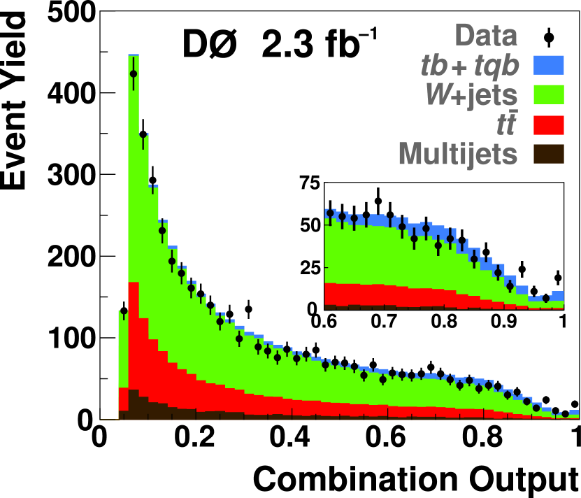
Figure 46: The combined discriminant for the D0 analysis.

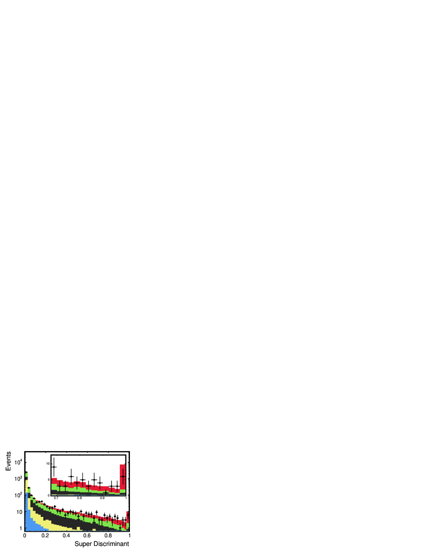
Figure 47: The combined discriminant for the CDF analysis

	$\sigma_{st}=\sigma_{s}+\sigma_{t}$
	D0	CDF
ME	$4.40^{+0.99}_{-0.79}$	$2.5^{+0.7}_{-0.8}$
LF	—	$1.6^{+0.8}_{-0.7}$
(B)NN	$4.70^{+1.18}_{-0.93}$	$1.8\pm 0.6$
BDT	$3.74^{+0.95}_{-0.79}$	$2.1^{+0.7}_{-0.8}$
LFS	—	$1.5^{+0.9}_{-0.8}$
$\mbox{$E\kern-6.00006pt\raise 0.43057pt\hbox{/}_{T}$}+\mathrm{jets}$	—	$4.9^{+2.6}_{-2.2}$
Combined	$3.94\pm 0.88$	$2.3^{+0.6}_{-0.5}$
Predicted [127]	$\sigma_{st}=3.46\pm 0.18$ for $M_{t}=170\ {\rm GeV/c}^{2}$
Predicted [80]	$\sigma_{st}=3.14\pm 0.31$

Table 26: Single top cross section measurements from the Tevatron (in pb). The D0 result used $M_{t}=170\ {\rm GeV/c}^{2}$ in simulations and calculation. The CDF result used $M_{t}=175\ {\rm GeV/c}^{2}$. The predicted cross section changes by 0.1 pb for a 5 ${\rm GeV/c}^{2}$ change in $M_{t}$ in this region.

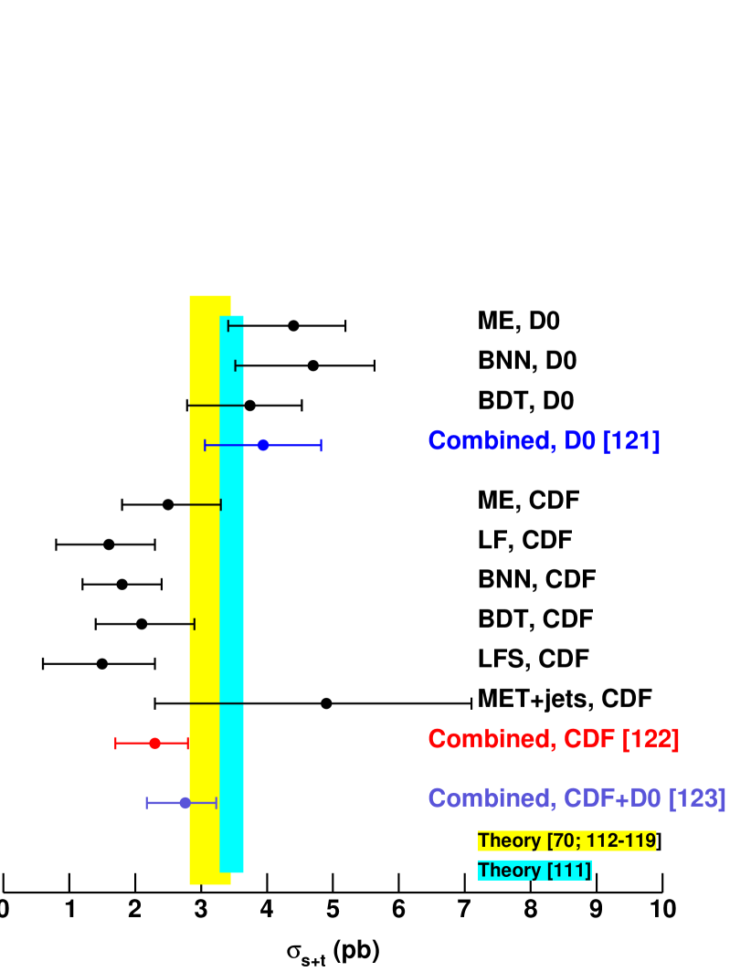
Figure 48: Ideogram of the single top cross section measurements from D0 and CDF.

The SM cross section is proportional to $|V_{tb}|^{2}$, so the cross section results are used to measure $|V_{tb}|$. The only assumption is that $|V_{tb}|\gg|V_{ts}|,|V_{td}|$ such that there is not a significant contribution to the signal from initial-state $s$ or $d$ quarks being transformed into top quarks via a $t$-channel $W$ boson. These results are shown in Tab. 27. The measured single top cross section is in good agreement with the SM prediction with $|V_{tb}|\simeq 1$.

D0	CDF
$|V_{tb}|>0.78$	$|V_{tb}|>0.71$
$|V_{tb}|=1.07\pm 0.12$	$|V_{tb}|=0.9\pm 0.11$

Table 27: $|V_{tb}|$ values extracted from the single top cross section measurements. The first row is the 95% CL result when no constraint is placed on on $|V_{tb}|$, and the second row is the result with the SM constraint $0\leq|V_{tb}|\leq 1$.

The precision of these results is limited by the statistics of the data samples. Both experiments are expected to continue these analyses through the end of the Tevatron running. In the most optimistic scenario this will result in analyzed data samples of up to $10$ fb^-1. Assuming the results in Table 27 scale as $1/\sqrt{\int{\cal L}~{}dt}$, the uncertainty on $|V_{tb}|$ will be reduced approximately two fold.

V HIGGS BOSON

V.1 Precision Electroweak Constraints

As discussed in Sections II.1 and II.2, the standard model, with the $SU(2)_{\rm L}\otimes U(1)_{Y}$ symmetry spontaneously broken via the vacuum-expectation value of a single Higgs-doublet field, is consistent with precision electroweak data. These data are so precise that they are sensitive to the mass of the Higgs boson at one loop, despite the fact that the Higgs mass enters only logarithmically. Fig. 49 shows the constraints on the Higgs-boson mass from both precision electroweak measurements (the blue band) and direct searches (the yellow areas). The precision data depend on the extrapolation of the fine-structure constant $\alpha$ from its measured value at low energy up to high energy, which suffers from an uncertainty associated with the contribution of low-energy QCD to the extrapolation. The solid black line indicates the central value, and the blue band takes into account all uncertainties. An alternative central value, associated with a different treatment of low-energy QCD, is indicated by the red dashed line. The effect on the central value by including the NuTeV data, which has some tension with the other precision electroweak data, is shown by the dotted magenta line.

It is striking that the precision data strongly prefer a Higgs boson mass in the 100 ${\rm GeV/c}^{2}$ region, while a purely theoretical analysis would accommodate a Higgs boson as heavy as about 700 ${\rm GeV/c}^{2}$ [133]. Taken at face value, the precision data indicate the Higgs boson is not much heavier than the current lower bound of $m_{H}>114\ {\rm GeV/c}^{2}$. It is also remarkable that the Tevatron experiments have succeeded in excluding the region $163\ {\rm GeV/c}^{2}<m_{H}<166\ {\rm GeV/c}^{2}$.

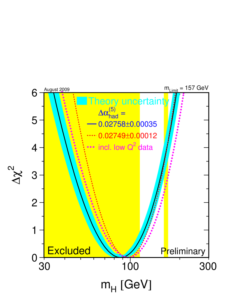
Figure 49: The $\Delta\chi^{2}$ as a function of assumed Higgs mass resulting from fits to data assuming the SM. The exclusion regions from direct searches are also shown.

V.2 Direct Searches

The experimental strategy and sensitivity to discover the standard model Higgs boson at the Tevatron through direct searches depends strongly on the value of $m_{H}$. For direct searches, the sensitive range is limited to $m_{H}\mathrel{\hbox to0.0pt{\raise 2.20013pt\hbox{$<$}\hss}{\lower 2.20013pt\hbox{$\sim$}}}250~{}{\rm GeV/c}^{2}$ where there exists sufficient center-of-mass collision energy at the parton-level for an appreciable rate of Higgs boson production via the gluon fusion ($ggH$) process which proceeds via a virtual quark loop (dominated by the top quark) [134].

For $m_{H}\mathrel{\hbox to0.0pt{\raise 2.20013pt\hbox{$<$}\hss}{\lower 2.20013pt\hbox{$\sim$}}}135~{}{\rm GeV/c}^{2}$ (the “low mass Higgs” region), the dominant Higgs decay is to $b$-quark pairs. The next largest contribution to the Higgs decay in the low mass Higgs region is $H\to\tau\tau$ which has a branching ratio of $\sim 7$%. In the case of $H\to bb$, the $ggH$ production is not useful to the direct Higgs search even using the $bb$ invariant mass because of overwhelming continuum $bb$ production. Instead, the associated vector boson ($VH$) process where the Higgs boson is produced in association with a $W$ or $Z$ boson is used. The additional leptons which can result from decay of the vector boson via $W\to\ell\nu$, $Z\to\ell\ell$ or $Z\to\nu\nu$ with $\ell=e,\,\mu$ [135; 136], whether detected directly or indirectly through $E\kern-6.00006pt\raise 0.43057pt\hbox{/}_{T}$, can be used suppress backgrounds at the expense of a lower cross section for $VH$ as compared to $ggH$.

The cross section and cross section times branching fraction for several Higgs masses in the low mass Higgs region  [137] are shown in Tab. 28. In addition to the modes listed in Tab. 28, the $WH\to WWW\to\ell^{\pm}\ell^{+^{\prime}}\ell^{-^{\prime}}$ channel provides some sensitivity in the transition region around $m_{H}\approx 135\ {\rm GeV/c}^{2}$ and vector boson fusion (VBF) $qq\rightarrow qqH$ and $ggH$ modes provide sensitivity in $\tau\bar{\tau}$ final states.

$m_{H}$ (${\rm GeV/c}^{2}$)	$\sigma(p\overline{p}\to WH)$	$\sigma\times B(W\to\ell\nu)$	$\sigma(p\overline{p}\to ZH)$	$\sigma\times B(Z\to\ell\ell)$	$\sigma\times B(Z\to\nu\nu)$
100	286	63.6	167	11.2	33.4
110	209	46.4	124	8.35	24.8
120	153	34.0	92.7	6.24	18.5
130	115	25.5	70.9	4.77	14.2

Table 28: The production cross section and cross section times branching fraction for the low mass ($m_{H}<135\ {\rm GeV/c}^{2}$) Higgs boson search. Cross sections are in femtobarns. For the final states denoted $\ell\nu$ and $\ell\ell$, the branching fraction used is the sum of $\ell=e\,\mu$.

For the low mass associated production channels $VH$ in which the $W$ or $Z$ boson decay involves one or two charged lepton(s), an initial sample consistent with production of a vector boson decaying to charged and/or neutral leptons and having at least two jets is selected. This sample has very low signal-to-noise but is already dominated by vector boson events and therefore provides a control sample used to validate detector modeling and rate predictions of the dominant backgrounds in the final analysis.

The requirement that one or more of the jets in the event is consistent with production of a $B$ hadron is added to the selection, dramatically reducing the contribution from the initially dominant $Vjj$ background and increasing the signal purity. Non-linear multivariate techniques for each final state are used to combine kinematic properties into a (typically) single variable in which a potential Higgs signal and backgrounds populate different regions. The distributions of these variables are then used as input to binned likelihood fits in which signal and background fractions are allowed to float within constraints of the total yield, predicted background contributions and all uncertainties. The absence (presence) of a significant signal resulting from the fits determines the mass limit (indicates discovery).

The low mass Higgs searches using the $ZH\to\nu\nu bb$ channel and final states involving one or two $\tau$ lepton decays follow different strategies. The $ZH\to\nu\nu bb$ channel has significant background from multijet QCD processes without real vector boson decay in which mismeasurement of jets results in significant $E\kern-6.00006pt\raise 0.43057pt\hbox{/}_{T}$. In this channel, an additional step (described later in this section) is added to improve an understanding of this background. The search using final states that involve either one or two $\tau$ leptons does not make use of $b$–jet identification since the $\tau$ leptons can arise either from Higgs boson decay or from $W$ or $Z$ decay.

The latest low mass Higgs searches from CDF and D0 are described in Section V.2.5. The most recent combination of low mass results, which includes some preliminary results not presented here, is described in Sections V.3– V.2.4.

For $m_{H}\mathrel{\hbox to0.0pt{\raise 2.20013pt\hbox{$>$}\hss}{\lower 2.20013pt\hbox{$\sim$}}}135~{}{\rm GeV/c}^{2}$ (the “high mass Higgs” region), the dominant Higgs decay is to $W$ boson pairs with the next largest contribution being $H\rightarrow ZZ^{(\ast)}$. Aside from a region around $m_{H}=150~{}{\rm GeV/c}^{2}$ where $BR(H\rightarrow ZZ^{(\ast)})$ peaks to $\sim 10$%, the $H\rightarrow WW^{(\ast)}$ decay where one of the final state $W$ bosons is off-shell for $M_{H}$ less than twice the $W$ mass completely dominates over the sensitive region of the Tevatron. The Higgs production cross section and branching fractions for several Higgs masses in the high mass region are shown in Table 29. The standard model Higgs boson branching fraction to $WW^{*}$ varies from 7.5% at 115 ${\rm GeV/c}^{2}$ to 73.5% at 200 ${\rm GeV/c}^{2}$ with a maximum of 96.5% at $\approx$ 170 ${\rm GeV/c}^{2}$ [134]. For $M_{H}\sim 170\;{\rm GeV/c}^{2}$, the standard model Higgs boson decays almost exclusively to two on-shell $W$ bosons, making this a region where the Tevatron has the best chance at a discovery or an exclusion.

$m_{H}$ (${\rm GeV/c}^{2}$)	$\sigma(gg\to H)$	$\sigma($VBF$)$	$B(H\to WW)$
150	548	45.7	0.682
160	439	38.6	0.901
170	349	33.6	0.965
180	283	28.6	0.934

Table 29: The production cross section and cross section times branching fraction for the high mass ($m_{H}>135\ {\rm GeV/c}^{2}$) Higgs boson search. Cross sections are in femtobarns.

At the Tevatron, the most sensitive Higgs search channel over the range $135~{}{\rm GeV/c}^{2}\mathrel{\hbox to0.0pt{\raise 2.20013pt\hbox{$<$}\hss}{\lower 2.20013pt\hbox{$\sim$}}}m_{H}\mathrel{\hbox to0.0pt{\raise 2.20013pt\hbox{$<$}\hss}{\lower 2.20013pt\hbox{$\sim$}}}200~{}{\rm GeV/c}^{2}$ is $gg\rightarrow H\rightarrow WW^{(*)}\rightarrow\ell\nu\ell\nu$, where the two charged leptons in the final state are of opposite charge [138; 139]. The $\ell\nu\ell\nu$ final state represents 6.0% of all $WW^{*}$ decays, where $\ell$ is either an electron or a muon, including those from $\tau$ leptons produced in the $W$ decays. Over the last few years, the experimental search for a high mass Higgs in decay to $WW$ at the Tevatron has evolved substantially to include powerful multivariate techniques and additional $H\rightarrow WW^{(\ast)}$ processes such as VBF $H\rightarrow WW^{(\ast)}$ and $VH(\rightarrow WW^{(*)})$. The latest high mass Higgs searches in the $H\rightarrow WW^{(\ast)}$ channel from CDF and D0 are described in Section V.2.5. A combination of these these results are described in Section V.3.

The following sections describe the individual channels used in the Higgs search starting with the low mass channels, $WH\to\ell\nu bb$, $ZH\to\ell\ell bb$, $ZH\to\nu\nu bb$ and $\tau$ final states, and finishing with the high mass $H\to WW^{(*)}\to\ell\nu\ell\nu$ search. The Higgs boson section concludes with a presentation of the most recent set of CDF and D0 combined limits.

V.2.1 $WH\to\ell\nu bb$ Final State

This final state has the largest cross-section times branching ratio of the entries shown in Tab. 28, and it also gives the most sensitivity to Higgs boson production for $M_{H}\mathrel{\hbox to0.0pt{\raise 2.20013pt\hbox{$<$}\hss}{\lower 2.20013pt\hbox{$\sim$}}}135\;{\rm GeV/c}^{2}$. Both CDF [140] and D0 [141] have carried out searches in this final state. The currently published results for D0 use a sample of $\int{\cal L}~{}dt=1.0$ fb^-1. The CDF published results use a sample of $\int{\cal L}~{}dt=2.1$ fb^-1, and preliminary results have been reported by both collaborations which use up to approximately $\int{\cal L}~{}dt=4$ fb^-1. The search strategies used by the two collaborations in the $WH$ channel are generally similar.

The initial event selection requires one high-$p_{T}$ electron or muon, large $E\kern-6.00006pt\raise 0.43057pt\hbox{/}_{T}$ and two or more jets. This selection mirrors the $\ell$, $\nu$ and $bb$ pair present in the final state. CDF requires the events to be selected by a trigger based on the presence of a high-energy electron or muon. The D0 analysis requires $\ell=e$ events to be selected by single–electron or electron plus jet triggers. For the muon final state D0 uses a two phase trigger selection. In the first phase, the events are required to be selected based on at least one of a set of single lepton or single-lepton plus jet triggers, and all yields are predicted and compared with data. After establishing agreement in this pass, the analysis is repeated allowing events to be selected by any trigger. The yield increases by an amount predicted by the inefficiency of the triggers for the first pass and all kinematic distributions remain in agreement after a simple yield scaling to 100% trigger efficiency.

At this stage, the dominant event source is $W$+jets with the jets arising from light quark ($u$, $d$, $s$, $c$) production. The signal-to-background is then improved by requiring one or two of the jets in the event to be identified as consistent with $b$ quark production. The D0 $b$ identification algorithm [142] uses a Neural Network (NN). The NN is trained and verified on a combination of data and simulation, with the critical efficiencies and misidentification rates determined from data control samples. The CDF analysis used three different $b$ identification algorithms. Jets are $b$-tagged by one or more algorithms based on the presence of a secondary vertex (secvtx) [143], a neural network [144], or signed impact parameters (JP)[145].

The signal purity is greatest when two $b$ jets are required, but this introduces significant efficiency loss compared to the case in which only one $b$ jet is required. To gain the most sensitivity, both categories of events, single $b$-tagged and double $b$-tagged, are retained, but they are analyzed separately. Optimization studies indicate that for the single-tag channel, rather restrictive tagging requirement is needed to control the background contribution from events with light-flavor (lf) jets misidentified as $b$ jets while for the double-tag channel, a less stringent requirement suffices thereby giving increased per–jet tagging efficiency. The D0 single-tag analysis uses a $b$–tag operating point which gives a typical efficiency of 48% with misidentification rate of 0.5% and an operating point for the double-tag analysis which gives an efficiency of 59% and a misidentification rate of 1.7%. The CDF event selection divides events into three exclusive categories based on which algorithms identify a jet as $b$-tagged. The first category contains events which have two jets tagged by the secvtx algorithm. The second category contains events not selected into the first category which have one jet identified by the secvtx algorithm and one by the jet probability algorithm. The third category contains events which are not selected into either of the other two categories and have one jet identified by both the secvtx and NN algorithms.

The sensitivity of the analyses are further improved by using kinematic properties of the events to distinguish signal and background events. The most important variable is the mass of the dijet system corresponding to the Higgs decay. For single-tagged events, the mass is computed using the tagged jet and the highest $p_{T}$ jet remaining, and for the double-tagged events the mass is computed using the two tagged jets. In addition to the mass, other variables can also distinguish signal and background on a statistical basis. To make best use of these, both experiments use a neural network to enhance the separation of signal and background in the final step of the analysis. The CDF neural network has six input variables and the D0 network have seven input variables. The variables used by each experiment are listed in Tab. 30 for comparison. Because of limited statistics in the $W$+three-jet sample, D0 uses the NN only for $W$+2 jet case and uses the dijet mass for the $W$+3 jet case.

CDF	00000000000000 D0 00000000000000
0000 $M_{JJ+}$ - invariant mass of $J_{1}$ and $J_{2}$ 0000	$M_{JJ}$ - invariant mass of $J_{1}$ and $J_{2}$
and the closest loose jet if $\Delta R(J,J_{loose})<0.9$
$\Sigma E_{T}$(loose jets)	$E_{T}(J_{1})$
$p_{T}(J_{1})+p_{T}(J_{2})+pT(\ell)-\mbox{$E\kern-6.00006pt\raise 0.43057pt\hbox{/}_{T}$}$	$E_{T}(J_{2})$
$M_{\ell\nu j}^{min}$	$\Delta R(J_{1},J_{2})$
$\Delta R(\ell,\nu_{max})$	$\Delta\phi(J_{1},J2)$
$|\vec{p}_{T}(\ell)+\vec{p}_{T}(\mbox{$E\kern-6.00006pt\raise 0.43057pt\hbox{/}_{T}$})+\vec{p}_{T}(J_{1})+\vec{p}_{T}(J_{2})|$	$|\vec{p}_{T}(\ell)+\vec{p}_{T}(\mbox{$E\kern-6.00006pt\raise 0.43057pt\hbox{/}_{T}$})|$
	$|\vec{p}_{T}(J_{1})+\vec{p}_{T}(J_{2})|$

Table 30: The neural network inputs for the CDF and D0 $WH$ analyses. Here $J_{i}$ denotes the $i$-th jet in a list ordered by jet $E_{T}$ in which $J_{1}$ is the highest $E_{T}$ jet in the event. $M_{\ell\nu j}^{min}$ is the mass of the lepton, $E\kern-6.00006pt\raise 0.43057pt\hbox{/}_{T}$ and the jet ($J_{1}$ or $J_{2}$) which gives the lower mass value. Finally, $\nu_{max}$ is the three momentum of the neutrino in which $|p_{Z}|$ is the larger of the two values calculated when forcing the lepton and neutrino system to have a mass equal to the $W$ boson mass.

Backgrounds to the $WH$ search include $W$+jets production (including jets arising from heavy flavor (hf) production), $t\overline{t}$, single top, diboson production ($WW$, $WZ$ and $ZZ$) and a small contribution from multijet events in which either the lepton is actually a jet misidentified as a lepton or the lepton arises from heavy flavor decay and the jet energy is not reconstructed so the lepton appears to be isolated. Both experiments estimate the $t\overline{t}$, single top and diboson yields using the product of the theoretical (N)NLO cross–section for each process, the luminosity and acceptance times efficiency for each process. Corrections are applied based on comparison of data and simulated control samples. The $W$+jets background cross sections are poorly known, and data–driven approaches are used to estimate these yields. The multijet background is hard to model from simulation, so data–driven methods are also used for this background. The two experiments use different data–driven methods as outlined below.

The total $W$+jets background after $b$–tagging in the CDF result is estimated separately for $W$+lf events and $W$+hf events. The $W$+lf contribution is estimated by applying data–derived mistag probabilities to untagged $W$+jets samples. Three different tagging algorithms are used in the analysis, and the mistag probability determination differs for each of these. For the secvtx and JP tagging algorithms, the mistag probability [143; 145] is derived using events with a negative decay length with a correction applied to account for the heavy-flavor content of the control sample used to determine the mistag probability. For the JP algorithm, the mistag probability is parametrized as a function of $\eta$, primary vertex $z$ position, jet $E_{T}$, scalar transverse energy, and vertex and track multiplicity. For the $NN$–based tagging algorithm, a light–flavor rejection factor derived from control data samples is used. The $W$+hf contribution is determined by measuring the heavy flavor faction in $W$+jets events and applying a $b$–tagging efficiency to these events. The initial heavy flavor fraction is derived from alpgen and pythia simulation and is corrected by a factor of $1.4\pm 0.4$ derived from a jet control data sample. The $b$–tagging efficiencies are determined from simulation and checked using control data samples.

The $W$+jets background yields after $b$–tagging in the D0 result are fixed by normalizing the simulated events to the untagged $W$+jets data after subtracting the other backgrounds from the data. The relative contributions of the $W$+lf, $W+c\overline{c}$, and $W+bb$ in the untagged sample are fixed to the cross-section ratios predicted by mcfm. The yields in the $b$–tagged sample are then computed by applying flavor–based (mis)identification probabilities to the jets in simulated events. The probabilities (one for $u$-, $d$- and $s$- quark initiated-jets, one for $c$-quark initiated jets and for for $b$-quark initiated jets) are derived using data control samples [142] and are parametrized as functions of jet $p_{T}$ and $\eta$.

The small background from multijet events is difficult to simulate accurately, so this component is also determined from control data samples. For CDF, a control sample is selected using events which have non-isolated leptons and low $E\kern-6.00006pt\raise 0.43057pt\hbox{/}_{T}$, and the yield in the signal sample is determined by extrapolating the yield from this sample into the signal region having isolated leptons and high $E\kern-6.00006pt\raise 0.43057pt\hbox{/}_{T}$. For D0, this background is determined by selecting a multijet dominated control sample with kinematics similar to the $WH$ events, and then applying a probability that these events would be misidentified and appear in the signal sample. The multijet control sample is selected by requiring lepton candidates which pass very loose isolation requirements, and the background yield is computed by applying the event–by-event probability that these loose–isolation events would pass the standard isolation requirement and thus appear in the signal sample.

Tab. 31 shows the data yields and background and signal predictions for the CDF analysis, and Tab. 32 shows the yields for the D0 analysis. The predicted Higgs yield includes not only $WH$ events, but also a small contribution from $ZH\to\ell\ell bb$ events in which one of the leptons ($\ell$) is not identified and thus generates $E\kern-6.00006pt\raise 0.43057pt\hbox{/}_{T}$ and a final state consistent with the $WH$ final state.

	Central region			Plug region
Pretag Events	32242			5879
$b$-tagging	ST+ST	ST+JP	ST+NN	ST+ST	ST+JP	ST+NN
Mistag	3.88$\pm$0.35	11.73$\pm$0.92	107.1$\pm$9.38	1.00$\pm$0.18	3.18$\pm$0.49	28.47$\pm$3.30
$Wbb$	37.93$\pm$16.92	31.15$\pm$14.03	215.6$\pm$92.34	7.40$\pm$3.96	6.23$\pm$3.37	43.09$\pm$12.33
$Wcc$	2.88$\pm$1.25	7.87$\pm$3.43	167.0$\pm$62.14	0.96$\pm$0.49	1.53$\pm$0.81	33.37$\pm$9.55
$t\bar{t}$(6.7pb)	19.05$\pm$2.92	15.56$\pm$2.39	60.68$\pm$9.30	2.14$\pm$0.34	1.79$\pm$0.31	7.17$\pm$1.00
Single top(s-ch)	6.90$\pm$1.00	5.14$\pm$0.75	14.38$\pm$2.09	0.69$\pm$0.10	0.51$\pm$0.08	1.53$\pm$0.20
Single top(t-ch)	1.60$\pm$0.23	1.87$\pm$0.27	29.57$\pm$4.33	0.22$\pm$0.04	0.24$\pm$0.04	3.54$\pm$0.47
$WW$	0.17$\pm$0.02	0.93$\pm$0.11	15.45$\pm$1.91	0.01$\pm$0.01	0.12$\pm$0.04	3.00$\pm$0.20
$WZ$	2.41$\pm$0.26	1.84$\pm$0.20	7.59$\pm$0.81	0.58$\pm$0.06	0.42$\pm$0.05	1.62$\pm$0.09
$ZZ$	0.06$\pm$0.01	0.08$\pm$0.01	0.31$\pm$0.03	0.00$\pm$0.01	0.01$\pm$0.01	0.02$\pm$0.00
$Z\rightarrow\tau\tau$	0.25$\pm$0.04	1.29$\pm$0.20	7.27$\pm$1.12	0.00$\pm$0.01	0.01$\pm$0.01	0.24$\pm$0.03
non-$W$ QCD	5.50$\pm$1.00	9.55$\pm$1.73	184.7$\pm$33.04	1.16$\pm$0.44	1.51$\pm$0.55	18.34$\pm$5.54
Total Background	80.6$\pm$18.8	87.0$\pm$18.0	809.6$\pm$159.4	14.2$\pm$4.0	15.5$\pm$3.6	140.4$\pm$16.9
$WH$ signal (120 ${\rm GeV/c}^{2}$)	0.85$\pm$0.10	0.60$\pm$0.07	1.70$\pm$0.14	0.09$\pm$0.01	0.06$\pm$0.01	0.20$\pm$0.01
Observed Events	83	90	805	11	13	138

Table 31: The predicted and observed yields for the CDF 2 fb^-1 $WH$ search separated by detector region. This table is from Ref. [140]

	$W$	+	2 jet	$W$	+	$2$ jet	$W$	+	$3$ jet	$W$	+	$3$ jet
	1$b$-tag			2 $b$-tag			1 $b$-tag			2 $b$-tag
WH	2.8	$\pm$	0.3	1.5	$\pm$	0.2	0.7	$\pm$	0.1	0.4	$\pm$	0.1
$WZ$	34.5	$\pm$	3.7	5.3	$\pm$	0.6	9.1	$\pm$	1.0	1.7	$\pm$	0.2
$Wb\bar{b}$	268	$\pm$	67	54	$\pm$	14	87	$\pm$	22	22.7	$\pm$	5.7
$W$+jets	347	$\pm$	87	14.0	$\pm$	4.4	96	$\pm$	24	8.5	$\pm$	2.7
$t\bar{t}$	95	$\pm$	17	37.4	$\pm$	7.0	156	$\pm$	29	81	$\pm$	15
single $t$	49.4	$\pm$	9.0	12.4	$\pm$	2.3	15.7	$\pm$	2.9	6.7	$\pm$	1.2
m-jet	104	$\pm$	29	8.9	$\pm$	2.1	54	$\pm$	15	8.7	$\pm$	2.1
Total	896	$\pm$	177	132	$\pm$	27	418	$\pm$	76	129	$\pm$	24
Data	885			136			385			122

Table 32: The predicted and observed yields for the D0 1 fb^-1 $WH$ search. This table is from Ref. [141]

Both CDF and D0 derive their final result by comparing the predicted and observed spectra using binned likelihoods. For both experiments, the single-tag and double-tag samples are separated and their likelihoods combined for the final results. D0 further separates the samples into events with exactly two jets and events with three jets. When determining the final result, CDF uses the dijet mass as the input to their likelihood. D0 uses the NN output for the two jet events and the dijet mass for three jet events. The likelihood methods are described in section V.3.

Systematic uncertainties are evaluated by both experiments for trigger efficiency, lepton identification efficiency, $b$–jet (mis)identification efficiency, the jet identification efficiency and jet energy calibration, multijet background calculation method, luminosity, and theory cross sections used for background and signal event yield calculations. CDF additionally reports uncertainties from parton density functions and initial and final state radiation modeling. D0 reports an additional systematic from the $W$+jets simulation derived by comparing shapes of distributions of data and simulated events before $b$–tagging.

The CDF NN output distributions for the tagged event selections are shown in Fig.. 50. The D0 NN output distribution (two jet events) and dijet mass distribution (three jet events) are shown in Fig. 51. The CDF and D0 cross section limits for the $WH$ final state only are shown if Figs. 52 and 53 respectively. The result from combining the results for all low mass final states is shown in Section V.3.

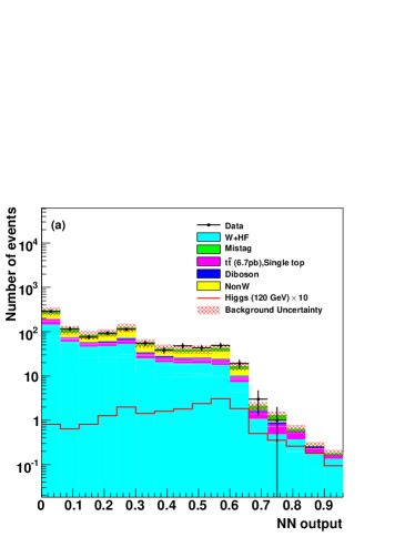
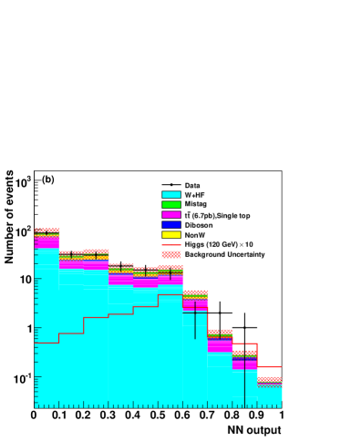
Figure 50: The NN output distributions for (a) single– (ST+NN) and (b) double–tagged (ST+ST, ST+JP) events from the CDF 2 fb^-1 $WH$ search.

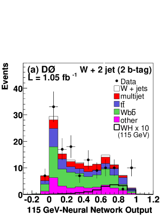
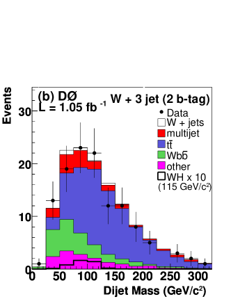
Figure 51: (a) The NN output for double-tagged dijet events and (b) the dijet mass for double-tagged three jet events from the D0 $WH$ search.

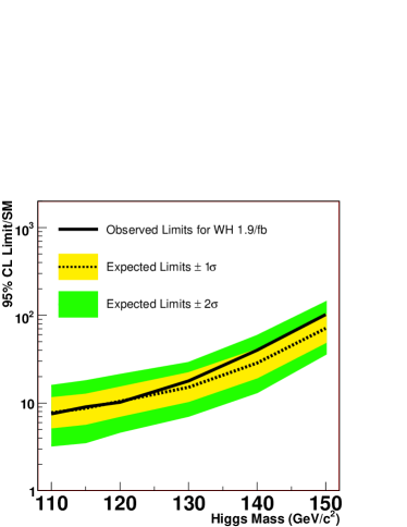
Figure 52: The cross section limits from the CDF $WH$ search.

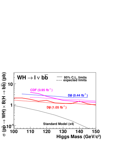
Figure 53: The cross section limits from the D0 $WH$ search.

V.2.2 $ZH\to\ell\ell bb$ Final State

The final state from $ZH\to\ell\ell bb$ events has the lowest production rate among those shown in Tab. 28 but has the highest purity. A similar strategy is taken for this final state as for the $WH$ final state. An initial sample of $Z$+dijet events is selected, the purity is improved by requiring $b$ jets, and the final result is determined by using either the invariant mass distribution or the output of a neural network as inputs to a shape–based limit setting program. Both D0 [146] and CDF [147] have published results in this final state. The D0 publication uses a data sample corresponding to $\int{\cal L}~{}dt=0.45$ fb^-1. The CDF published results corresponds to $\int{\cal L}~{}dt=1.0$ fb^-1.

The initial selections for both experiments require events with two leptons whose invariant mass is consistent with a $Z$ boson and two additional jets. The backgrounds in this channel arise from $Z$+jets, $t\overline{t}$ events, diboson production, and from jets misidentified as leptons or a lepton+jet system being misidentified as an isolated lepton. They are determined using a combination of simulated events and data control samples in essentially the same manner as for the $WH$ channel. One difference with respect to the $WH$ calculation is that sidebands of the $\ell\ell$ invariant mass distribution are used by D0 to determine the misidentification and false isolation background. Both experiments identify $b$ jets using secondary vertex algorithms. The CDF result splits the final tagged sample into single- and double-tagged samples as in the $WH$ analysis, but the D0 result does not. The D0 result is derived using the dijet mass distribution only, while the CDF result is based on the binned likelihood of a NN output. The sources of systematic uncertainties for these channels are the same as for the $WH$ result. Tab. 33 shows the yields for the single- and double-tag analyses from CDF, and Tab. 34 shows the yields for the dijet and double-tagged samples for D0 respectively. Figure 54 (55) shows the dijet invariant mass (neural network output) distribution from the D0 (CDF) analysis. This distribution is used as the input to the limit setting program.

Source	Single-Tagged	Double-Tagged
$Z+bb$	$35.1\pm 14.6$	$6.3\pm 2.5$
$Z+c\overline{c}$	$21.8\pm 8.5$	$1.0\pm 0.4$
$Z+q\overline{q}$	$32.3\pm 5.5$	$1.0\pm 0.2$
$t\overline{t}$	$5.2\pm 1.0$	$2.8\pm 0.6$
$ZZ$	$4.0\pm 0.8$	$1.3\pm 0.3$
$WZ$	$1.2\pm 0.2$	$0.04\pm 0.01$
Non-$Z$	$1.9\pm 1.4$	$0.2\pm 0.2$
Total Expected	$101.5\pm 32$	$12.7\pm 4.1$
Observed	100	11
Signal Yield	$0.44$	$0.23$

Table 33: Single- and double-tagged yields for the CDF 1.0 fb^-1 $ZH\to\ell\ell bb$ search.

Source	Dijet	Double-tagged
$Z+bb$	17.4	3.3
$Z+jj$	851	3.8
$t\overline{t}$	12.3	3.9
$WZ+ZZ$	30.6	0.74
Non-$Z$	44.1	0.59
Total Exp.	956	12.3
Observed	1008	15

Table 34: Dijet and double-tagged sample yields for the D0 0.45 fb^-1 $ZH\to\ell\ell bb$ search.

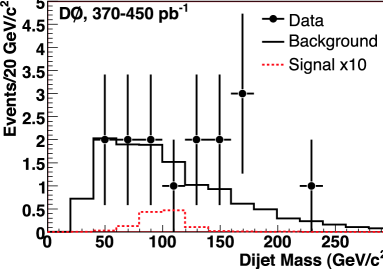
Figure 54: Dijet mass distribution for the D0 1.0 fb^-1 $ZH\to\ell\ell bb$ analysis.

Figure 55: NN distributions for the (a) single-tagged and (b) double-tagged samples from the CDF 1.0 fb^-1 $ZH\to\ell\ell bb$ analysis. The 95% CL upper bound cross section is 19$\times$ the SM prediction.

Systematic uncertainties are included for trigger and lepton identification efficiencies, parton density functions, background cross sections, $b$–tagging efficiencies, jet energy reconstruction and the methods used to estimate instrumental backgrounds. The CDF result also includes a systematic from the top mass uncertainty. The systematic uncertainties for the D0 measurement range between 2% and 20% expressed as a fraction of the total background. The systematic uncertainties for the CDF measurement range between 1% and roughly 25% of the total background. The largest contribution for both experiments is from the background cross sections.

The final limits, derived using the same methods as the $WH$ results, are shown for CDF in Fig. 56 and for D0 in Fig. 57. As expected these channels have considerably less sensitivity than the $WH$ channels because of the significantly lower signal cross-section times branching fraction.

Figure 56: Expected and Observed limits for the CDF 1.0 fb^-1 $ZH\to\ell\ell bb$ analysis.

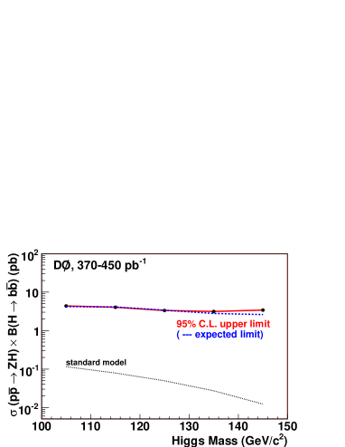
Figure 57: Expected and Observed limits for the D0 0.45 fb^-1 $ZH\to\ell\ell bb$ analysis.

V.2.3 $ZH\to\nu\nu bb$ and Related Final States

The $ZH\to\nu\nu bb$ final state has a production rate intermediate between the $WH$ and $ZH\to\ell\ell bb$ final states. This final state also has a significant contribution from the process $WH\to\ell\nu bb$ in which the charged lepton $\ell$ escapes detection. This is particularly true for the case $\ell=\mu$ because the muon leaves very little energy in the calorimeter and thus results in event $E\kern-6.00006pt\raise 0.43057pt\hbox{/}_{T}$ similar to that from $Z\to\nu\nu$ decay.

Unlike either of the previously discussed final states, the $ZH\to\nu\nu bb$ final state has no charged leptons from vector boson decay. This implies a significantly increased background from SM multijet events in which $E\kern-6.00006pt\raise 0.43057pt\hbox{/}_{T}$ arises from mismeasurement. This background is difficult to model from simulation, and analyses of this final state must develop techniques to measure it using data control samples. Both CDF [148] and D0 [149] have published results in this final state. The two experiments have developed different methods for controlling and estimating the multijet background.

CDF Search

The CDF analysis uses a data sample corresponding to 1 fb^-1 and begins with selection of events passing a $E\kern-6.00006pt\raise 0.43057pt\hbox{/}_{T}$ trigger with level one $\mbox{$E\kern-6.00006pt\raise 0.43057pt\hbox{/}_{T}$}>25$ GeV, a level two requirement of two jet clusters having $E_{T}>10$ GeV and a level three requirement of $\mbox{$E\kern-6.00006pt\raise 0.43057pt\hbox{/}_{T}$}>35$ GeV. At least one of the level two jets must also satisfy $\eta<1.1$. The initial offline selection (“pre-tag”) requires events to have $MET>50$ GeV and exactly two jets with $E_{T}>20$ GeV. One of the jets must have $E_{T}>35$ GeV, and the other must have $E_{T}>25$ GeV. Additionally, one of the jets must satisfy $|\eta|<0.9$, and the other jet must satisfy $|\eta|<2.4$. The two jets must also have $\Delta\phi>1.0$ rad, and events with high $p_{T}$, isolated leptons are vetoed. Finally, at least one of the jets is required to have a secondary vertex $b$–tag

All non-multijet backgrounds; $t\overline{t}$, $W$+jets, $Z$+jets and diboson production are modeled using simulated events. The multijet background is studied by dividing the sample into two control regions and a signal region. The regions are defined in Tab. 35. The multijet background in all regions is divided into two components: (1) events with only light-flavor ($u$, $d$ and $s$) quarks in which one or more of the jets is misidentified with a secondary vertex and (2) events with $c$ and $b$ quarks. The contribution from light flavor jets is determined using a control sample with no tags to which a misidentification factor is applied. The heavy flavor contribution is determined using simulated events with normalization factors for single-tag and double-tag topologies determined by forcing the data yields and the sum of all backgrounds to agree (before dividing the sample into the three regions). The scale factors are $1.30\pm 0.4$ ($1.47\pm 0.07$) for the single(double) $b$–tagged events.

	Dominant
Region	Source	Selection
CR1	Multijet	Leptons Vetoed
		$\Delta\Phi(\vec{E}_{T2},\vec{}\mbox{$E\kern-6.00006pt\raise 0.43057pt\hbox{/}_{T}$})<0.4$
CR2	EW, $t\overline{t}$	Lepton Required
		$\Delta\Phi(\vec{E}_{T2},\vec{}\mbox{$E\kern-6.00006pt\raise 0.43057pt\hbox{/}_{T}$})>0.4$
Signal		Leptons Vetoed
		$\Delta\Phi(\vec{E}_{T1},\vec{}\mbox{$E\kern-6.00006pt\raise 0.43057pt\hbox{/}_{T}$})>0.4$
		$\Delta\Phi(\vec{E}_{T2},\vec{}\mbox{$E\kern-6.00006pt\raise 0.43057pt\hbox{/}_{T}$})>0.4$

Table 35: Definitions of the three regions (CR1, CR2, and Signal) in the CDF $VH\to\mbox{$E\kern-6.00006pt\raise 0.43057pt\hbox{/}_{T}$}bb$ search. $\Delta\Phi(\vec{E}_{T1(2)},\vec{}\mbox{$E\kern-6.00006pt\raise 0.43057pt\hbox{/}_{T}$})$ is the angle between the $E\kern-6.00006pt\raise 0.43057pt\hbox{/}_{T}$ and the jet with the highest(second highest) $E_{T}$.

The final analysis selection is determined by optimizing $S/\sqrt{(}B)$ where $S$ is the total signal yield, including the contribution from $WH\to\ell\nu bb$ in which the lepton is not identified, and $B$ is the total background. The optimization is carried out only for the signal region. The final selection then requires $\Delta\phi(j_{1},j_{2})>0.8$, $\mbox{$H\kern-6.00006pt\raise 0.43057pt\hbox{/}_{T}$}/H_{T}>0.454$, $E_{T}^{j_{1}}>60$ GeV and $\mbox{$E\kern-6.00006pt\raise 0.43057pt\hbox{/}_{T}$}>70$ GeV. Here $H_{T}$ is the scalar sum of the jet $E_{T}$ values, $H\kern-6.00006pt\raise 0.43057pt\hbox{/}_{T}$ is the magnitude of the vector sum and $j_{1}$($j_{2}$) denotes the jet with the highest(second highest) $E_{T}$.

The systematic uncertainties arise from a number of sources. For the CDF analysis the dominant uncertainty in the jet energy calibration which varies between 10% - 26% for multijet and $V$+jets (including heavy flavor) backgrounds, but is only 8% for signal events. The other dominant systematic arises from the calculated cross sections used to normalize backgrounds. This ranges between 11% - 40% for a given source depending on the samples. The total systematic is 17% for the single–tagged analysis and 19% for the double-tagged analysis.

Fig. 58 shows dijet invariant mass for the single- and double-tagged events in the signal region. The yields are given in Tab. 36. The limits on Higgs production are calculated using the same procedure as for the previous two channels, and they are shown in Fig. 59.

Source	Signal–tagged	Double–tagged
Multijet	$93\pm 23$	$3.74\pm 1.27$
$t\overline{t}$	$27.3\pm 3.8$	$4.88\pm 0.8$
Diboson	$7.0\pm 1.4$	$0.79\pm 0.19$
$W+$hf	$33.4\pm 16.2$	$1.65\pm 0.86$
$Z$+hf	$18.3\pm 8.1$	$1.67\pm 0.77$
Mistags	$69\pm 9$	$1.64\pm 0.48$
Total	$248\pm 43$	$14.4\pm 2.7$
Observed	268	16

Table 36: Yields in the CDF $VH\to\mbox{$E\kern-6.00006pt\raise 0.43057pt\hbox{/}_{T}$}bb$ analysis.

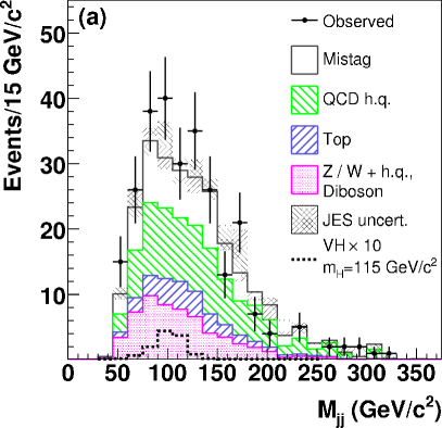
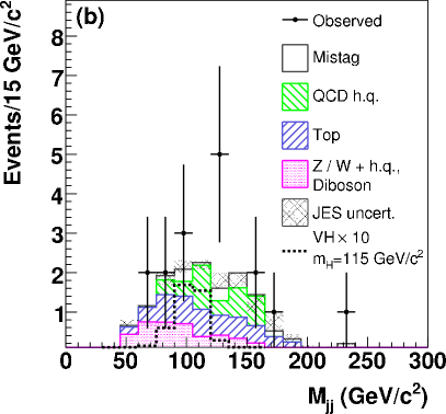
Figure 58: The dijet invariant mass distributions for the (a) single-tagged and (b) double–tagged CDF searches in the $VH\to\mbox{$E\kern-6.00006pt\raise 0.43057pt\hbox{/}_{T}$}bb$ final state.

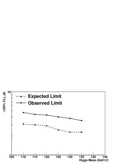
Figure 59: Expected and observed 95% CL upper bounds on the $VH$ production cross section for the CDF $\mbox{$E\kern-6.00006pt\raise 0.43057pt\hbox{/}_{T}$}+bb$ search.

D0 Search

The published D0 analysis uses a data sample corresponding to $\int{\cal L}~{}dt=5.2$ fb^-1. Events selected for this analysis must satisfy a trigger requiring two acoplanar jets and $E\kern-6.00006pt\raise 0.43057pt\hbox{/}_{T}$ in which the kinematic thresholds varied as a function of the instantaneous luminosity. The primary requirements of the initial offline event preselection are at least two jets with $E_{T}>20$ GeV and $|\eta|<2.5$, $\Delta\phi(j_{1},j_{2})<165^{o}$, and $\mbox{$E\kern-6.00006pt\raise 0.43057pt\hbox{/}_{T}$}>20$ GeV. This is divided into four samples: (1) a signal sample defined by the additional requirements of $\mbox{$E\kern-6.00006pt\raise 0.43057pt\hbox{/}_{T}$}>40$ GeV, $S>5$, $D<\pi/2$ and a veto of events with high-$p_{T}$, isolated leptons, (2) an electroweak test sample enhanced in $W\to\mu\nu$ events and defined similarly as for the signal sample, but requiring the presence of a high $p_{T}$, isolated muon, (3) a multijet modeling sample defined similarly to the signal sample except $D>\pi/2$ and (4) a multijet enriched sample used to confirm the background model predicted using the multijet modeling sample and defined by $\mbox{$E\kern-6.00006pt\raise 0.43057pt\hbox{/}_{T}$}>30$ GeV and no requirement on $S$. Here $S$ is the significance of the $E\kern-6.00006pt\raise 0.43057pt\hbox{/}_{T}$ and $D\equiv\Delta\phi(\vec{\mbox{$E\kern-6.00006pt\raise 0.43057pt\hbox{/}_{T}$}},\vec{\mbox{$T\kern-6.00006pt\raise 0.43057pt\hbox{/}_{T}$})}=\phi_{\mbox{$E\kern-4.20004pt\raise 0.3014pt\hbox{/}_{T}$}}-\phi_{\mbox{$T\kern-4.20004pt\raise 0.3014pt\hbox{/}_{T}$}}$ in which $T\kern-6.00006pt\raise 0.43057pt\hbox{/}_{T}$ is the magnitude of the vector sum of the transverse momentum of the tracks in the event and $\phi_{i}$ is the azimuthal angle of either $E\kern-6.00006pt\raise 0.43057pt\hbox{/}_{T}$ or $T\kern-6.00006pt\raise 0.43057pt\hbox{/}_{T}$.

The presence of $b$ hadrons from the $H\to bb$ signal decay is used to improve the signal to noise. Events were additionally required to have a least one of the two highest $E_{T}$ jets identified as being consistent with a $b$ hadron jet as determined by a high purity (tight) $b$-jet identification requirement. Events are then categorized as double–tagged if the remaining one of the two highest $E_{T}$ jets satisfies a lower purity (loose) identification requirement. Events without an additional tag are denoted single–tagged. For the tight requirement, the per jet identification efficiency is 50% with a misidentification probability of 0.5%. The loose requirement has an efficiency of 70% with a misidentification probability of 6.5%. Tab. 37 shows the data yield and prediction for the initial preselection and for the single– and double–tagged samples and the expected Higgs boson signal for a Higgs boson of mass $115~{}{\rm GeV/c}^{2}$.

Sample	$ZH$	$WH$	$W$+jets	$Z$+jets	Top	$VV$	Multijet	Total background	Observed
Preselection	13.73 $\pm$ 1.37	11.64 $\pm$ 1.17	19 069	9432	1216	1112	1196	32 025 $\pm$ 4037	31 718
Single–tagged	4.16 $\pm$ 0.42	3.60 $\pm$ 0.37	802	439	404	60	125	1830 $\pm$ 255	1712
Double–tagged	4.66 $\pm$ 0.58	4.00 $\pm$ 0.50	191	124	199	24	$<8$	538 $\pm$ 87	514

Table 37: The predicted and observed yields for the D0 $VH\to\mbox{$E\kern-6.00006pt\raise 0.43057pt\hbox{/}_{T}$}bb$ analysis for the untagged control sample and the single– and double–tagged analysis samples after applying the multijet BDT selection.

The backgrounds from $t\overline{t}$, $W$+jets, $Z$+jets and diboson processes are estimated using simulated events. These results are validated using the EW enriched control sample. The shape of the multijet background is taken from the multijet modeling sample, and the normalization is determined by forcing the number of multijet events plus the number of SM predicted background events to equal the data yield in the preselection sample. This procedure is validated by comparing the prediction with the multijet enriched sample.

The signal-to-background separation is then further improved using boosted decision trees (BDTs). For each $m_{H}$ considered, a multijet boosted decision tree (MJ BDT) with 23 input variables is trained on Higgs signal and multijet backgrounds. Events which have a MJ BDT output greater than 0.6 are retained. These events are then input to a second BDT (SM BDT) trained on the remaining backgrounds and Higgs signal events using the same 23 variables input to the MJ BDT. Fig. 60 shows the BDT outputs for the data, predicted background and signal. The agreement between data and prediction is good. Limits are extracted by fitting signal and background SM BDT outputs to the data distribution using the same modified frequentist algorithm as was used for the previously described D0 results. Fig. 61 shows the Higgs cross section limits from the D0 analysis.

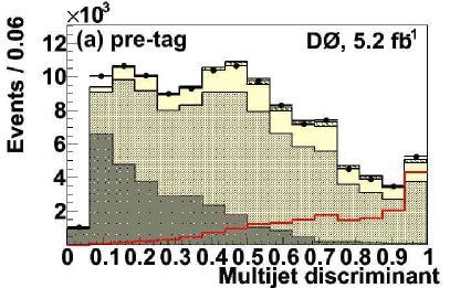
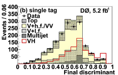
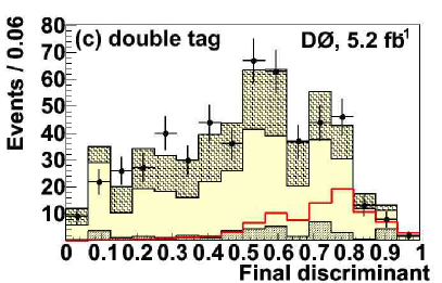
Figure 60: The outputs for the (a) MJ BDT, (b) the SM BDT for the single–tagged channel and (c) the SM BDT for the double–tagged channel for the D0 $VH\to\mbox{$E\kern-6.00006pt\raise 0.43057pt\hbox{/}_{T}$}bb$ analysis.

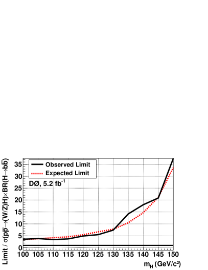
Figure 61: The expected and observed 90% CL upper bounds on the Higgs boson production cross section in the D0 $VH\to\mbox{$E\kern-6.00006pt\raise 0.43057pt\hbox{/}_{T}$}bb$ search.

The systematic uncertainties for the D0 result are dominated by similar sources as for the CDF analysis. The D0 jet energy calibration systematic is $<10$%, and the background normalization systematic varies between 6% - 20%. D0 also reports additional systematic uncertainties from luminosity, trigger and identification efficiencies and $b$-tagging efficiency. These sources have an uncertainty of roughly 5% for each.

V.2.4 $\tau+$jets and $\tau\tau$+jets Final States

The searches described earlier for the processes $WH\to\ell\nu bb$ and $ZH\to\ell\ell bb$ required $\ell=e,\,\mu$, but corresponding channels exist with $\ell=\tau$ leptons in the final state. In addition, B$(H\to\tau\tau)\approx 7\%$ in the SM, the most important mode after $H\to bb$. D0[150] has published searches for Higgs production in the modes $VH\to\tau bb\to\tau_{h}\nu$ and $VH\to\tau\tau jj\to\mu\nu\nu_{\tau}\tau_{h}jj$, $p\overline{p}\to VVjj\to Hjj\to\tau\tau jj\to\mu\nu\nu_{\tau}\tau_{h}jj$, and $gg\to Hjj\to\tau\tau jj\to\mu\nu\nu_{\tau}\tau_{h}jj$ using a data sample corresponding to 1.0 $fb^{-1}$. Here $\tau_{h}$ represents a $\tau$ decay to hadrons.

The primary signal contribution to the $\tau\nu\nu bb$ final state comes from $WH\to\tau\nu bb$, but roughly 7% of the final signal acceptance comes from $ZH\to\tau\tau bb$ in which one $\tau$ is not identified. The identified $\tau$ is required to decay to hadrons [58]. Candidate events are initially selected using a trigger requiring a high $p_{T}$ jet and large $E\kern-6.00006pt\raise 0.43057pt\hbox{/}_{T}$. The offline selection requires a hadronic $\tau$ decay, with a minimum transverse energy from 12 ${\rm GeV/c}$ to 20 ${\rm GeV/c}$, with the range depending in which of two decay topologies the $\tau$ lepton is reconstructed. The topologies correspond roughly to single charged-hadron $\tau$ lepton decays (type 1) and single charged-hadron with multiple neutral-hadron decays (type 2). In addition to the $\tau$ lepton candidate, the basic offline selection requires $\mbox{$E\kern-6.00006pt\raise 0.43057pt\hbox{/}_{T}$}>30$ GeV, the presence of at least two candidate $b$-jets with $p_{T}>20\ {\rm GeV/c}$ and $|\eta|<2.5$, $\leq 3$ jets with $p_{T}\ {\rm GeV/c}$, and a veto of events with a high-$p_{T}$ electron or muon to keep orthogonality with the other searches. Events are also required to pass $\Delta\phi(\mbox{$E\kern-6.00006pt\raise 0.43057pt\hbox{/}_{T}$},\mbox{$T\kern-6.00006pt\raise 0.43057pt\hbox{/}_{T}$})<\pi/2$, $H_{T}<200$ GeV, $50<M_{JJ}<200\ {\rm GeV/c}^{2}$, and $\Delta\phi(\tau,\mbox{$E\kern-6.00006pt\raise 0.43057pt\hbox{/}_{T}$})<0.02(\pi-2)(\mbox{$E\kern-6.00006pt\raise 0.43057pt\hbox{/}_{T}$}-30)+2$. In addition, for events with type 2 tau decay, the transverse mass of the $\vec{\tau}$ and $\vec{\mbox{$E\kern-6.00006pt\raise 0.43057pt\hbox{/}_{T}$}}$ must satisfy $M_{T}<80\ {\rm GeV/c}^{2}$.

The $\tau\tau jj$ final state search has signal contributions from a variety of processes: $ZH\to\tau\tau bb$, $ZH\to q\overline{q}bb$ (in which $H\to\tau\tau$, VBF $p\overline{p}\to VVjj\to Hjj\to\tau\tau jj\to\mu\nu\nu_{\tau}\tau_{h}jj$, and gluon fusion $gg\to Hjj\to\tau\tau jj\to\mu\nu\nu_{\tau}\tau_{h}jj$. Unlike other low mass channels, some of these processes have no $b$–quarks in the decay chain. Consequently, no $b$-jet identification is required for this search. One of the $\tau$ leptons is required to decay to hadrons, and the other $\tau$ lepton is required to decay to a muon. Here three topologies are used. Two of these are the same as in the $\tau\nu bb$ search, and the third corresponds roughly to $\tau$ lepton decays to three charged hadrons. Candidate events are initially selected by requiring at least one trigger from a set of single muon and muon plus jet triggers. The initial offline selection requires a muon with $p_{T}>12\ {\rm GeV/c}$ and $\eta<2.0$, a hadronic $\tau$ lepton decay candidate with a minimum transverse energy from 15 GeV to 20 GeV (again depending on topology) and at least two jets with $p_{T}>15\ {\rm GeV/c}$ and $\eta|<2.5$. No $b$-jet identification is used. Signal and background separation is then improved using a set of neutral networks. A separate neutral network is trained for each of the four signal sources ($WH$, $ZH\ (H\to bb)$, $ZH\ (H\to\tau\tau)$ and $VBF$), paired with each of the main backgrounds ($W+$jets, $Z+$jets, $t\overline{t}$ and multijet). In addition separate networks are trained for low mass (105, 115 and 125 ${\rm GeV/c}^{2}$) and high mass (135, 145 ${\rm GeV/c}^{2}$) giving a total of 32 networks. Each network uses six or seven input variables chosen such that each one individually improves the $S/\sqrt{B}$ when it is added as the last variable. The same choice of input variables is made at all masses for each signal and background pairing.

All backgrounds except that from multijet events in which jets are misidentified as $\tau$ leptons are estimated using simulated events processed through a detailed detector simulation with corrections based on comparison of data and simulated control samples. The absence of electrons and muons from direct $W$ or $Z$ decay results in a significantly higher multijet background in this search than in most. The multijet background is estimated from using a control data sample enriched in $\tau$-like hadronic jet events. Systematic uncertainty sources include trigger efficiency, lepton and jet identification efficiencies, jet energy calibration and production cross section uncertainties for backgrounds determined using simulated events.

As for the other analyses, systematic uncertainties are divided into those which affect only normalization and those which affect the shape. Sources affecting the normalization include: the integrated luminosity, the trigger efficiency, muon identification efficiency, $\tau$ lepton identification efficiency, jet identification efficiency, the $\tau$ lepton energy calibration and background cross sections. The systematic uncertainties which affect the shape for the $\tau\nu bb$ analysis are the jet energy resolutions, the jet energy calibration and the $b$–tagging efficiencies. For the $\tau\tau jj$ analysis only the multijet background had a shape dependence. The systematic uncertainties, expressed as a fraction of the related source, range between 3% and 30%. For example, the $W$+hf cross section systematic is 30% of the $W$+hf background, but because the background is roughly 50% of the total background in the $\tau\nu bb$ channel, the effective systematic is roughly 15%.

Predicted background and signal levels and observed yields for the two searches are shown in Tab. 38 assuming a signal mass of $M_{H}=115\ {\rm GeV/c}^{2}$. The distributions or $M_{JJ}$ and the output from the $Z+$jets NN $NN_{Z}$ are used as inputs to the limit setting program for the $\tau\nu bb$ and $\tau\tau jj$ searches respectively. The distributions are shown in Fig. 62, and the resulting limits are shown in Tab. 39.

	Search Channel
Source	$\tau\nu bb$	$\tau\tau jj$
$W+$lf	$0.5\pm 0.0$	$5.1\pm 0.3$
$W+$hf	$10.9\pm 0.3$	$0.9\pm 0.1$
$Z+$lf	$<0.2$	$43.8\pm 0.6$
$Z+$hf	$0.4\pm 0.0$	$10.1\pm 0.7$
$t\overline{t}$	$9.5\pm 0.1$	$2.8\pm 0.0$
Diboson	$0.7\pm 0.0$	$2.1\pm 0.2$
Multijet	$1.3\pm 0.1$	$6.5\pm 2.8$
Total	$23.3\pm 0.4$	$71.2\pm 3.0$
Data	$13$	$58$
Signal	$0.216$	$0.293$

Table 38: Expected and observed yields for the D0 $VH\to\tau\nu bb$ and $VH\to\tau\tau jj$ searches. Only statistical uncertainties are shown.

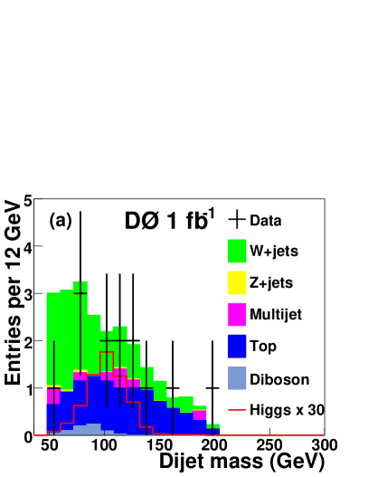
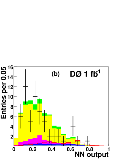
Figure 62: The dijet invariant mass distribution for the D0 $VH\to\tau\nu bb$ search, and the NN output for the $VH\to\tau\tau jj$ search.

	$\tau\nu bb$		$\tau\tau jj$		Combined
$M_{H}$ (${\rm GeV/c}^{2}$)	exp.	obs.	exp.	obs.	exp.	obs.
105	33	27	39	36	24	20
115	42	35	43	47	28	29
125	62	60	60	65	40	44
135	105	106	87	61	63	50

Table 39: Expected and observed 95% CL signal cross–section upper limits for the D0 $VH\to\tau\nu bb$ and $VH\to\tau\tau jj$ searches. The limits are given as a ratio of the cross–section limit to the SM cross–section prediction.

V.2.5 $H\rightarrow WW^{*}$

For $m_{H}\mathrel{\hbox to0.0pt{\raise 2.20013pt\hbox{$>$}\hss}{\lower 2.20013pt\hbox{$\sim$}}}135~{}{\rm GeV/c}^{2}$, the dominant Higgs decay is to $W$ boson pairs. Below the $W$ pair production threshold, one of the $W$ bosons will be off-shell which leads to lower $p_{T}$ leptons from the $W^{*}$ decay. The most sensitive high mass Higgs channel is $gg\rightarrow H\rightarrow WW^{(*)}\rightarrow\ell\nu\ell\nu$, where the two charged leptons in the final state of are of opposite charge. In addition to the dominant $ggH$ process, other Higgs production processes that contribute at the Tevatron are VBF and $VH$ where $V\equiv(W,Z$).

Early Tevatron Run II searches for a high mass Higgs boson [151],[152] focused mainly on the $ggH$ process and exploiting the angular correlation between final state charged leptons due to the scalar (spin-0) nature of the SM Higgs. In a more recent analysis [153], CDF used a NN technique to search for a Higgs boson signal in dilepton + $E\kern-6.00006pt\raise 0.43057pt\hbox{/}_{T}$ events having either zero or one reconstructed jet. Several kinematic variables, including the results of matrix element calculations that combined charged lepton and $E\kern-6.00006pt\raise 0.43057pt\hbox{/}_{T}$ information, were used as inputs to the NN.

The CDF and D0 searches for $H\rightarrow WW^{(\ast)}$ in [154] and [155], respectively, significantly increase their sensitivities compared to previous results through the use of additional data, topologies arising from VBF and $VH$ channels, and analysis improvements such as increased charged lepton acceptance (D0).

In the D0 analysis [155], an integrated luminosity of 5.4 $~{}\rm{fb}^{-1}$ is used to search for $H\rightarrow WW^{(\ast)}$ in events with two oppositely-charged leptons $e^{+}e^{-}$, $e^{\pm}\mu^{\mp}$, or $\mu^{+}\mu^{-}$. Electrons are required to have $|\eta|<2.5$ ($<2.0$ in the $e^{+}e^{-}$ channel) and $E_{T}^{e}>15$ GeV. Muons are required to have $|\eta|<2.0$ and $p_{T}^{\mu}>10~{}{\rm GeV/c}$ (in the $\mu^{+}\mu^{-}$ channel, one of the two muons is required to have $p_{T}^{\mu}>20~{}{\rm GeV/c}$). In addition, the dilepton invariant mass is required to exceed $15~{}{\rm GeV/c}^{2}$. Reconstructed jets are required to have $E_{T}^{\rm jet}>15$ GeV and $|\eta|<2.4$, however no jet-based event selection is applied since the number of jets in the event is used as input to an NN to help discriminate signal from background. The dilepton invariant mass after this “preselection” is shown in Fig. 63(a).

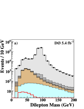
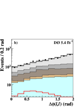
Figure 63: For the D0 $H\rightarrow WW^{(\ast)}$ analysis [155], the (a) dilepton invariant mass after preselection; (b) $\Delta\phi(\ell,\ell)$ angle after final selection; and (c) neural network output after final selection. The signal is shown for $m_{H}$=165 GeV. The systematic uncertainty is shown after the fit.

Additional cuts are made to suppress $Z/\gamma^{*}$ production. These include requiring $\mbox{$E\kern-6.00006pt\raise 0.43057pt\hbox{/}_{T}$}>20$ GeV ($>25$ GeV in the $\mu^{+}\mu^{-}$ channel), high quality $E\kern-6.00006pt\raise 0.43057pt\hbox{/}_{T}$ measurement, a minimum $W$ transverse mass to be $>20$ GeV ($>30$ GeV in the $e^{+}e^{-}$ channel), and azimuthal opening angle between the two leptons $\Delta\phi(\ell,\ell)<2.0$ rad.

To improve the separation between signal and background, a NN optimized for several $m_{H}$ values between $115~{}{\rm GeV/c}^{2}$ and $200~{}{\rm GeV/c}^{2}$ is used in each of the three channels. Several discriminant variables are used as inputs to the NN: the transverse momenta of the leptons, a variable indicating the quality of the leptons’ identification, the transverse momentum and invariant mass of the dilepton system, minimum $W$ transverse mass, $E\kern-6.00006pt\raise 0.43057pt\hbox{/}_{T}$, $E\kern-6.00006pt\raise 0.43057pt\hbox{/}_{T}$ quality, $\Delta\phi(\ell,\ell)$, $\Delta\phi(\ell_{1},\mbox{$E\kern-6.00006pt\raise 0.43057pt\hbox{/}_{T}$})$, $\Delta\phi(\ell_{2},\mbox{$E\kern-6.00006pt\raise 0.43057pt\hbox{/}_{T}$})$, the number of identified jets, and the scalar sum of the transverse momenta of the jets.

Fig. 63 shows the agreement between data and Monte Carlo simulation after final selection for (b) the $\Delta\phi(\ell,\ell)$ angle and (c) the neural network output. The expected and observed event yields are shown in Tab. 40.

	$e^{\pm}\mu^{\mp}$			$e^{+}e^{-}$			$\mu^{+}\mu^{-}$
	Preselection	Final selection		Preselection	Final selection		Preselection	Final selection
$Z/\gamma^{*}\to e^{+}e^{-}$	120	$<0.1$		274886	158$\,\pm\,$	13	$-$	$-$
$Z/\gamma^{*}\to\mu^{+}\mu^{-}$	89	4.3$\,\pm\,$	0.3	$-$	$-$		373582	1247$\,\pm\,$	37
$Z/\gamma^{*}\to\tau^{+}\tau^{-}$	3871	7.1$\,\pm\,$	0.5	1441	0.7$\,\pm\,$	0.1	2659	12.0$\,\pm\,$	0.7
$t\overline{t}$	312	93.8$\,\pm\,$	8.3	159	47.0$\,\pm\,$	4.4	184	74. 6$\,\pm\,$	6.8
$W+{\rm jets}/\gamma$	267	112$\,\pm\,$	9	308	122$\,\pm\,$	11	236	91.5$\,\pm\,$	6.5
$WW$	455	165$\,\pm\,$	6	202	73.9$\,\pm\,$	6.4	272	107$\,\pm\,$	9
$WZ$	23.6	7.6$\,\pm\,$	0.2	137	11.5$\,\pm\,$	1.0	171	21.5$\,\pm\,$	2.0
$ZZ$	5.4	0.6$\,\pm\,$	0.1	117	9.3$\,\pm\,$	0.9	147	18.0$\,\pm\,$	1.8
Multijet	430	6.4$\,\pm\,$	2.5	1370	1.0$\,\pm\,$	0.1	408	53.8$\,\pm\,$	10.3
Signal ($m_{H}=165$ GeV)	18.8	13.5$\,\pm\,$	1.5	11.2	7.2$\,\pm\,$	0.8	12.7	9.0$\,\pm\,$	1.0
Total background	5573	397$\,\pm\,$	14	278620	423$\,\pm\,$	19	377659	1625$\,\pm\,$	41
Data	5566	390		278277	421		384083	1613

Table 40: Expected and observed event yields in each channel after preselection and at the final selection for the D0 $H\rightarrow WW^{(\ast)}$ analysis [155]. The systematic uncertainty after fitting is shown for all samples at final selection.

No significant excess of signal-like events is observed for any test value of $m_{H}$ after the final selection. The NN output distributions are used to set upper limits on the SM Higgs boson production cross section. Fig. 64(a) shows a comparison of the NN distribution between background-subtracted data and the expected signal for $m_{H}=165~{}{\rm GeV/c}^{2}$ hypothesis. Fig. 64(b) shows the expected and observed upper limits as a ratio to the expected SM cross section. Assuming $m_{H}=165~{}{\rm GeV/c}^{2}$, the observed (expected) upper limit at 95% CL on Higgs boson production is a factor of 1.55 (1.36) times the SM cross section.

Figure 64: For the D0 $H\rightarrow WW^{(\ast)}$ analysis [155], the (a) data after subtracting the fitted background (points) and SM signal expectation (filled histogram) as a function of the NN output for $m_{H}=165~{}{\rm GeV/c}^{2}$. Also shown is the $\pm 1$ standard deviation (s.d.) band on the total background after fitting. (b) Upper limit on Higgs boson production cross section at 95% CL expressed as a ratio to the SM cross section. The one and two s.d. bands around the curve corresponding to the background-only hypothesis are also shown.

In the CDF analysis [154], an integrated luminosity of 4.8 $~{}\rm{fb}^{-1}$ is used to search for $H\rightarrow WW^{(\ast)}$ in events with either an opposite sign (OS) or same-sign (SS) charged lepton pair. This is an inclusive search that expands the signal acceptance by 50% for $m_{H}=160~{}{\rm GeV/c}^{2}$ compared to searching for only the $ggH$ production process as published previously by CDF [153].

The CDF analysis uses physics objects identified as jets, electrons, and muons as well as the $E\kern-6.00006pt\raise 0.43057pt\hbox{/}_{T}$ in events. The search is based on the requirement that events contain two charged leptons resulting from the decays of the final-state vector bosons which are OS except in the case of the $VH$ channel where they can be SS. At least one charged lepton is required to match the lepton found in the trigger and have $E_{T}(p_{T})>20$ GeV (${\rm GeV/c}$) for electrons (muons). The second charged lepton is required to have $E_{T}(p_{T})>10$ GeV (${\rm GeV/c}$) except in events with same charge leptons, where both leptons are required to have $E_{T}(p_{T})>20$ GeV (${\rm GeV/c}$). Requirements on the event $E\kern-6.00006pt\raise 0.43057pt\hbox{/}_{T}$ indicative of the presence of neutrinos from $W$ boson decay are made in opposite-charge dilepton events. Backgrounds due to Drell-Yan and heavy flavor are suppressed by requiring that the invariant mass of the lepton pair be greater than $16~{}{\rm GeV/c}^{2}$. The Higgs boson signature can also involve jets of hadrons produced from the decay of one of the vector bosons in the $VH$ process, forward quarks in the VBF process, or from the radiation of gluons.

In order to increase the sensitivity to the various Higgs production processes in the SM, candidate events are subdivided into six analysis channels based on jet multiplicity, lepton categories, and lepton charge combinations. Five of the channels have signatures with OS leptons and the other is for SS leptons.

Discrimination of signal from background is based on NNs trained in each analysis channel and at each of 14 hypothesized $m_{H}$ values in the range $110\leq m_{H}\leq 200~{}{\rm GeV/c}^{2}$. The NN inputs are based on kinematic quantities selected to exploit features such as the spin correlation between the $W$ bosons in Higgs boson decay, the presence of large $E\kern-6.00006pt\raise 0.43057pt\hbox{/}_{T}$ from the neutrinos; the transverse mass of the Higgs boson (calculated using the leptons’ four-momenta and $E\kern-6.00006pt\raise 0.43057pt\hbox{/}_{T}$ vector); and the modest total energy of the Higgs boson decay products compared to $t\overline{t}$ decay. In the zero jet categories, we additionally classify events by evaluating the observed kinematic configuration in a likelihood ratio of the signal probability density divided by the sum of the signal and background probability densities. These probability densities are determined from LO matrix element calculations of the cross sections of each process [153] (see also Section III.5.4 for the case of SM $WW$).

An example NN discriminant distribution for the combination of all categories is shown in Fig. 65, where signal and background expectations for a $160~{}{\rm GeV/c}^{2}$ Higgs boson are compared to the observed data.

Figure 65: The combined distribution of NN scores for backgrounds and a $M_{H}=160~{}{\rm GeV/c}^{2}$ Higgs boson compared to the observed data shown with statistical uncertainties for the CDF $H\rightarrow WW^{(\ast)}$ analysis [154]. The Higgs boson distribution is normalized to ten times the SM expectation.

No significant excess of events beyond SM background expectations in the NN discriminant are observed. The 95% confidence limits on $\sigma_{H}$, expressed as a ratio to the expected SM rate as a function of $m_{H}$, are determined from the data. The median expected and observed upper limits on $\sigma_{H}$ as a function of $m_{H}$ is shown in Fig. 66.

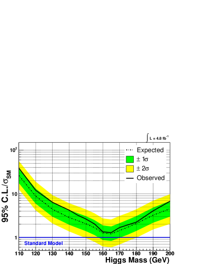
Figure 66: Expected and observed upper limits at the 95% CL on $\sigma_{H}$ presented as a ratio to the predicted SM values as a function of $M_{H}$ for the CDF $H\rightarrow WW^{(\ast)}$ analysis [154]. The dashed line represents the median expected limits, the green and yellow bands the estimated one and two sigma probability bands for the distribution of expectations, and the solid line the observed limit.

The expected and observed upper limits at 95% CL for Higgs boson production cross section expressed as a ratio to the cross section predicted by the SM as a function of $m_{H}$ for the CDF and D0 searches for $H\rightarrow WW^{(\ast)}$ in [154] and [155], respectively, is shown in Tab. 41.

Table 41: Expected and observed upper limits at 95% CL for Higgs boson production cross section expressed as a ratio to the cross section predicted by the SM for a range of test Higgs boson masses.

	$m_{H}$ (GeV)	120	130	140	145	150	155	160	165	170	175	180	190	200
D0 [155]	Limit (exp.)	9.74	5.40	3.48	3.07	2.58	2.02	1.43	1.36	1.65	2.06	2.59	4.20	6.23
	Limit (obs.)	13.6	6.63	5.21	3.94	3.29	3.25	1.82	1.55	1.96	1.89	2.11	3.27	5.53
CDF [154]	Limit (exp.)	8.85	4.41	2.85	2.43	2.05	1.67	1.26	1.20	1.44	1.72	2.09	3.24	4.53
	Limit (obs.)	12.04	6.38	4.21	3.23	2.62	2.04	1.34	1.29	1.69	1.94	2.24	4.06	6.74

V.3 Combined Limits

Results for individual search final states are combined by the Tevatron New–Phenomena and Higgs Working Group[156]. The combinations are updated roughly every six months to one year using the most up to date preliminary and published results. The combination is performed using a joint probability density incorporating each channel as an individual result with systematic uncertainties and their correlations included. Two algorithms are used for the combination. One is a Bayesian approach[154], and the other is a modified frequentist approach[157; 158; 159]. In both algorithms, the impact of systematic uncertainties is reduced by treating these as nuisance parameters. Results for the 95% CL upper bound on the Higgs production cross section from the two algorithms agree to within 10%.

The most recent combination[137] incorporates published and preliminary results based on samples ranging from $\int{\cal L}~{}dt=2.1$ fb^-1 to $\int{\cal L}~{}dt=5.4$ fb^-1, and combined $H\rightarrow WW$ limits are at [160]. The cross section upper bounds are a factor of 2.7 higher than the SM prediction for $m_{H}=115$ ${\rm GeV/c}^{2}$ and production of a SM Higgs is excluded at the 95% CL in the region $163<m_{H}<166\ {\rm GeV/c}^{2}$. The results are shown in Fig. 67 expressed as a ratio of the 95% CL upper bound cross section divided by the SM prediction.

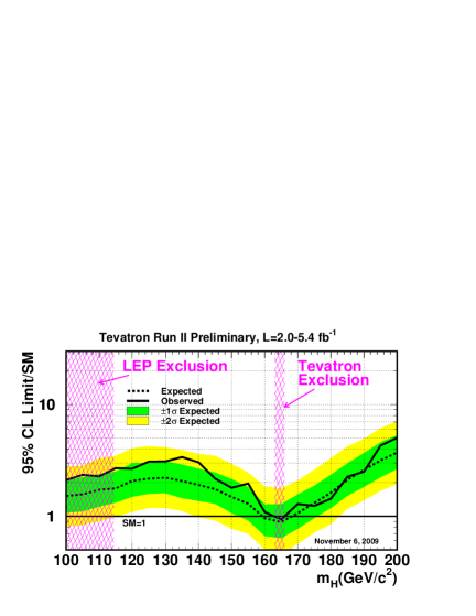
Figure 67: The 95% CL upper bounds on the Higgs production cross section divided by the predicted cross section. This result includes both published and preliminary results from CDF and D0.

VI SUMMARY AND OUTLOOK

The SM has been tested extensively over the last forty years. The only significant deviation from its predictions is the existence of neutrino mass. Ongoing studies of the SM are being carried out by the Tevatron experiments, CDF and D0. This paper presents results of these tests and discusses prospects for the remainder of the Tevatron running and the transition from the Tevatron to the LHC.

CDF and D0 have presented a wide variety of results relating to the EW sector. Among the results are observation of all SM diboson processes involving $W$, $Z$ and $\gamma$, including for the first time $WZ$ production, observation of EW production of single top quarks and the corresponding measurement of $|V_{tb}|$, world’s best measurements of the top quark and $W$ boson masses allowing improved indirect constraints on the Higgs boson mass, and ongoing searches for the Higgs boson which have begun to exclude mass values outside of the existing limits. In addition to testing the SM, some of these are benchmark measurements eventually to be compared with corresponding results from the LHC. Others, like the top quark and $W$ boson masses, are likely to be legacy measurements from the Tevatron.

With additional luminosity still to come for CDF and D0, many of these measurements will significantly improve before the end of Run II at the Tevatron. This is an exciting time in particle physics as the field transitions from the era of the Tevatron to an era of the LHC as the machine to probe physics at the energy frontier.

VII ACKNOWLEDGMENTS

The many beautiful experimental measurements summarized in this paper are the result of the work of thousands of people from the Fermilab accelerator division, CDF and D0. The authors wish to thank those involved in making these possible. In addition, the authors thank Andrew Askew, Tom Diehl, Reinhard Schwienhorst and Junjie Zhu for useful discussion and clarification.

References

- [1] T. Aaltonen et al. Phys. Rev. D, 99:151801, 2007.
- [2] V. M. Abazov et al. Nucl. Instrum. Methods Phys. Res., Sect. A, 565:463, 2006.
- [3] S. Weinberg. Phys. Rev. Lett., 43:1566, 1979.
- [4] W. Buchmuller and D. Wyler. Nucl. Phys., B268:621, 1986.
- [5] A. De Rujula, M. B. Gavela, P. Hernandez, and E. Masso. Nucl. Phys., B384:3, 1992.
- [6] K. Hagiwara, S. Ishihara, R. Szalapski, and D. Zeppenfeld. Phys. Rev., D48:2182, 1993.
- [7] G. Arnison et al. Phys. Lett., B122:103, 1983.
- [8] M. Banner et al. Phys. Lett., B122:476, 1983.
- [9] G. Arnison et al. Phys. Lett., B126:398, 1983.
- [10] P. Bagnaia et al. Phys. Lett., B129:130, 1983.
- [11] G. P. Abbiendi et al. Phys. Rept., 427:257, 2006.
- [12] M. Kober, B. Koch, and M. Bleicher. Phys. Rev., D76:125001, 2007.
- [13] R. Hamberg, W. L. van Neerven, and T. Matsuura. Nucl. Phys., B359:343, 1991.
- [14] A. D. Martin, R. G. Roberts, W. J. Sterling, and R. S. Thorne. Phys. Lett., B604:61, 2004.
- [15] J. Pumplin et al. J. High Energy Phys., 0207:12, 2002.
- [16] A. Abulencia et al. J. Phys., G34:2457, 2007.
- [17] A. Sirlin. Phys. Rev., D22:971, 1980.
- [18] S. Schael et al. Eur. Phys. J., C47:309, 2006.
- [19] J. Abdallah et al. Eur. Phys. J., C55:1, 2008.
- [20] P. Achard et al. Eur. Phys. J., C45:569, 2006.
- [21] G. Abbiendi et al. Eur. Phys. J., C45:307, 2006.
- [22] A. Affolder et al. Phys. Rev., D64:052001, 2001.
- [23] V. M. Abazov et al. Phys. Rev., D66:012001, 2002.
- [24] J. Alcaraz et al. arXiv:0911.2604 [hep-ex], 2009.
- [25] L. Lyons, D. Gibaut, and P. Clifford. Nucl. Instrum. Meth., A270:110, 1988.
- [26] A. Valassi. Nucl. Instrum. Meth., A500:391, 2003.
- [27] V. M. Abazov et al. Phys. Rev. Lett., 103:141801, 2009.
- [28] Tevatron Electroweak Working Group. arXiv:0908.1374 [hep-ex], 2009.
- [29] J. Rosner, M.. Worah, and T. Takeuchi. Phys. Rev., D49:1363, 1994.
- [30] T. Affolder et al. Phys. Rev. Lett., 85:3347, 2000.
- [31] V. M. Abazov et al. Phys. Rev., D66:032008, 2002.
- [32] T. Aaltonen et al. Phys. Rev. Lett., 100:071801, 2008.
- [33] V. M. Abazov et al. Phys. Rev. Lett., 103:231802, 2009.
- [34] V. M. Abazov et al. Nucl. Instrum. Meth., A609:250, 2009.
- [35] D. Acosta et al. Phys. Rev. D., 971:052002, 2005.
- [36] V. M. Abazov et al. Phys. Rev. Lett., 101:191801, 2008.
- [37] C. Amsler et al. Phys. Lett. B, 667:1, 2008.
- [38] G. P. Zeller et al. Phys. Rev. Lett., 88:091802, 2002.
- [39] K Hagiwara, R. D. Peccei, D. Zeppenfeld, and K. Hikasa. Nucl. Phys., B282:253, 1987.
- [40] K. Hagiwara, J. Woodside, and D. Zeppenfeld. Phys. Rev. D, 41(7):2113, 1990.
- [41] D. Zeppenfeld and S. Willenbrock. Phys. Rev. D, 37(7):1775, 1988.
- [42] U. Baur and D. Zeppenfeld. Physics Letters B, 201(3):383, 1988.
- [43] U. Baur and E. L. Berger. Phys. Rev., D47:4889, 1993.
- [44] U. Baur and D. L. Rainwater. Phys.Rev., D62:113011, 2000.
- [45] C. Quigg. Annual Review of Nuclear and Particle Science, 59:505, 2009.
- [46] D. Acosta et al. Phys. Rev. Lett., 94:041803, 2005.
- [47] V. M. Abazov et al. Phys. Rev., D71:091108, 2005.
- [48] V. M. Abazov et al. Phys. Rev. Lett., 100:241805, 2008.
- [49] U. Baur and E. L. Berger. Phys. Rev., D41:1476, 1990.
- [50] U. Baur, T. Han, and J. Ohnemus. Phys. Rev., D48:5140, 1993.
- [51] R. W. Brown, D. Sahdev, and K. O. Mikaelian. Phys. Rev. D, 20(5):1164, 1979.
- [52] K. O. Mikaelian, M. A. Samuel, and D. Sahdev. Phys. Rev. Lett., 43(11):746, 1979.
- [53] C. J. Goebel, F. Halzen, and J. P. Leveille. Phys. Rev. D, 23(11):2682, 1981.
- [54] S. Brodsky and R. Brown. Phys. Rev. Lett., 49(14):966, 1982.
- [55] U. Baur, S. Errede, and G. L. Landsberg. Phys.Rev., D50:1917, 1994.
- [56] V. M. Abazov et al. Phys. Lett., B653:378, 2007.
- [57] U. Baur, T. Han, and J. Ohnemus. Phys. Rev. D, 57(5):2823, 1998.
- [58] V. M. Abazov et al. Phys. Rev. Lett., 102:201802, 2009.
- [59] F. Abe et al. Phys. Rev. Lett., 78(24):4536, 1997.
- [60] V. M. Abazov et al. Phys. Rev. Lett., 94(15):151801, 2005.
- [61] D. Acosta et al. Phys. Rev. Lett., 94(21):211801, 2005.
- [62] T. Aaltonen et al. Phys. Rev. Lett., 104(20):201801, 2010.
- [63] V. M. Abazov et al. Phys. Rev. Lett., 103:191801, 2009.
- [64] J. M. Campbell and R. K. Ellis. Phys. Rev. D, 60(11):113006, 1999.
- [65] A. Abulencia et al. Phys. Rev. Lett., 98:161801, 2007.
- [66] V. M. Abazov et al. Phys. Rev. Lett., 95:141802, 2005.
- [67] V. M. Abazov et al. Phys. Rev., D76:111104, 2007.
- [68] J. Alcaraz et al. hep-ex/0612034, 2006.
- [69] V. M. Abazov et al. Phys. Rev. Lett., 100:131801, 2008.
- [70] T. Aaltonen et al. Phys. Rev. Lett., 100:201801, 2008.
- [71] V. M. Abazov et al. Phys. Rev. Lett., 101:171803, 2008.
- [72] V. M. Abazov et al. Phys. Rev. D, 78(7):072002, 2008.
- [73] V. M. Abazov et al. Phys. Rev. Lett., 102:161801, 2009.
- [74] T. Aaltonen et al. Phys. Rev. Lett., 104(10):101801, 2010.
- [75] T. Aaltonen et al. Phys. Rev., D76:111103, 2007.
- [76] V. M. Abazov et al. Phys. Rev., D80:053012, 2009.
- [77] L. Breiman. Mach. Learn., 45:5, 2001.
- [78] D. Acosta et al. Phys. Rev. Lett., 94:091803, 2005.
- [79] M. Cacciari et al. J. High Energy Phys., 09:127, 2008.
- [80] B. Harris, E. Laenen, L. Phaf, Z. Sullivan, and S. Weinzierl. Phys. Rev., D66:054024, 2002.
- [81] T. Aaltonen et al. Phys. Rev. Lett., 103:091803, 2009.
- [82] V. M. Abazov et al. arXiv:0907.4952 [hep-ex], 2009.
- [83] A. X. El-Khadra and M. Luke. Ann. Rev. Nucl. Part. Sci., 52:201, 2002.
- [84] M. Smith and S. Willenbrock. Phys. Rev. Lett., 79:3825, 1997.
- [85] T. Aaltonen et al. Phys. Rev. Lett., 102(15):152001, 2009.
- [86] V. M. Abazov et al. Phys. Rev., D80:092006, 2009.
- [87] T. Aaltonen et al. Phys. Rev., D79:072001, 2009.
- [88] V. M. Abazov et al. Phys. Rev. Lett., 101:182001, 2008.
- [89] R. Dalitz and G. Goldstein. Phys. Rev., D45:1531, 1992.
- [90] K. Kondo. J. Phys. Soc. Jpn., 57:4126, 1988.
- [91] K. Kondo. J. Phys. Soc. Jpn., 60:836, 1991.
- [92] B. Abbott et al. Phys. Rev. Lett., 80:2063, 1998.
- [93] B. Abbott et al. Phys. Rev., D60:052001, 1999.
- [94] T. Aaltonen et al. Phys. Rev. D, 79(9):092005, 2009.
- [95] Tevatron Electroweak Working Group. arXiv:0903.2503 [hep-ex], 2009.
- [96] U. Langenfeld, S. Moch, and P. Uwer. Phys. Rev. D, 80(5):054009, 2009.
- [97] T. Aaltonen et al. Phys. Rev., D79:072005, 2009.
- [98] T. Aaltonen et al. Phys. Rev. Lett., 100:062005, 2008.
- [99] A. Abulencia et al. Phys. Rev. D, 75:031105, 2007.
- [100] A. Abulencia et al. Phys. Rev. D, 75:071102, 2007.
- [101] V. M. Abazov et al. Phys. Rev. D, 75:092001, 2007.
- [102] A. Abulencia et al. Phys. Rev. Lett., 96:022004, 2006.
- [103] T. Aaltonen et al. Phys. Rev. D, 79(7):072010, 2009.
- [104] T. Aaltonen et al. Phys. Rev., D79:072010, 2009.
- [105] T. Aaltonen et al. Phys. Rev. D, 75:111103, 2007.
- [106] K. Fujikawa and A. Yamada. Phys. Rev. D, 49:5890, 1994.
- [107] P Cho and M. Misiak. Phys. Rev. D, 49:5894, 1994.
- [108] T. Aaltonen et al. Phys. Lett., B674:160, 2009.
- [109] V. M. Abazov et al. Phys. Rev. Lett., 100:062004, 2008.
- [110] T Sjostrand et al. Comput. Phys. Commun., 135:238, 2001.
- [111] M. L. Mangano, M. Moretti, F. Piccinini, R. Pittau, and P. Polosa. J. High Energy Phys., 07:1, 2003.
- [112] S. Abachi et al. Phys. Rev. Lett., 74:2632, 1995.
- [113] F. Abe et al. Phys. Rev. Lett., 74:2626, 1995.
- [114] S. Cortese and R Petronzio. Phys. Lett. B, 253:494, 1991.
- [115] T. Stelzer and S. Willenbrock. Phys. Lett. B, 357:125, 1995.
- [116] A.P. Heinson et al. Phys. Rev. D, 56:3114, 1997.
- [117] S. Willenbrock and D. Dicus. Phys. Rev. D, 34:155, 1986.
- [118] C. P. Yuan. Phys. Rev. D, 41:42, 1990.
- [119] K. Ellis and S. Parke. Phys. Rev. D, 46:3785, 1992.
- [120] T. Stelzer, Z. Sullivan, and S. Willenbrock. Phys. Rev., D56:5919, 1997.
- [121] M. Smith and S. Willenbrock. Phys. Rev., D54:6696, 1996.
- [122] Z. Sullivan. Phys. Rev. D, 70:114012, 2004.
- [123] J. Campbell, R. K. Ellis, and F. Tramontano. Phys. Rev., D70:094012, 2004.
- [124] Q.-H. Cao, R. Schwienhorst, and C.-P. Yuan. Phys. Rev., D71:054023, 2005.
- [125] Q.-H. Cao, R. Schwienhorst, J. A. Benitez, R. Brock, and C.-P. Yuan. Phys. Rev., D72:094027, 2005.
- [126] S. Frixione, E. Laenen, P. Motylinski, and B. R. Webber. JHEP, 03:092, 2006.
- [127] N. Kidonakis. Phys. Rev. D, 74:114012, 2006.
- [128] J.. Campbell, R. Frederix, F. Maltoni, and F. Tramontano. Phys. Rev. Lett., 102:182003, 2009.
- [129] V. M. Abazov et al. Phys. Rev. Lett., 98:181802, 2007.
- [130] V. M. Abazov et al. Phys. Rev. D, 78:012005, 2008.
- [131] T. Aaltonen et al. Phys. Rev. Lett., 101:252001, 2008.
- [132] Tevatron Electroweak Working Group. arXiv:0908.2171 [hep-ex], 2009.
- [133] M. Luscher and P. Weisz. Phys. Lett., B212:472, 1988.
- [134] A. Djouadi. Phys. Rept., 457:1, 2008.
- [135] A. Stange, W. J. Marciano, and S. Willenbrock. Phys. Rev., D49:1354, 1994.
- [136] A. Stange, W. J. Marciano, and S. Willenbrock. Phys. Rev., D50:4491, 1994.
- [137] The Tevatron New–Phenomena and Higgs Working Group. arXiv:0911.3930 [hep-ex], 2009.
- [138] T. Han and R.-J. Zhang. Phys. Rev. Lett., 82(1):25, 1999.
- [139] T. Han, A. S. Turcot, and R.-J. Zhang. Phys. Rev. D, 59(9):093001, 1999.
- [140] T. Aaltonen et al. Phys. Rev., D80:012002, 2009.
- [141] V. M. Abazov et al. Phys. Rev. Lett., 102:051803, 2009.
- [142] T. Scanlon. FERMILAB-THESIS-2006-43, 2006.
- [143] D. Acosta et al. Phys. Rev., D71:052003, 2005.
- [144] T. Aaltonen et al. Phys. Rev., D78:032008, 2008.
- [145] A. Abulencia et al. Phys. Rev., D74:072006, 2006.
- [146] V. M. Abazov et al. Phys. Lett., B655:209, 2007.
- [147] T. Aaltonen et al. Phys. Rev. Lett., 101:251803, 2008.
- [148] T. Aaltonen et al. Phys. Rev. Lett., 100:211801, 2008.
- [149] V. M. Abazov et al. Phys. Rev. Lett., 104(7):071801, 2010.
- [150] V. M. Abazov et al. Phys. Rev. Lett., 102:251801, 2009.
- [151] A. Abulencia et al. Phys. Rev. Lett., 97:081802, 2006.
- [152] V. M. Abazov et al. Phys. Rev. Lett., 96:011801, 2006.
- [153] T. Aaltonen et al. Phys. Rev. Lett., 102:021802, 2009.
- [154] T. Aaltonen et al. Phys. Rev. Lett., 104(6):061803, 2010.
- [155] V. M. Abazov et al. Phys. Rev. Lett., 104(6):061804, 2010.
- [156] Tevatron New-Phenomena and Higgs Working Group. http://tevnphwg.fnal.gov.
- [157] T. Junk. Nucl. Instrum. Meth., A434:435, 1999.
- [158] A. L. Read. J. Phys. G: Nucl. Part. Phys., 28:2693, 2002.
- [159] W. Fisher. 2006. FERMILAB-TM-2386-E.
- [160] T. Aaltonen et al. Phys. Rev. Lett., 104(6):061802, 2010.