The VIMOS-VLT Deep Survey:
Evolution in the Halo Occupation Number since z $\sim$ 1

Abstract

We model the evolution of the mean galaxy occupation of dark-matter halos over the range $0.1<z<1.3$, using the data from the VIMOS-VLT Deep Survey (VVDS). The galaxy projected correlation function $w_{p}(r_{p})$ was computed for a set of luminosity-limited subsamples and fits to its shape were obtained using two variants of Halo Occupation Distribution models. These provide us with a set of best-fitting parameters, from which we obtain the average mass of a halo and average number of galaxies per halo. We find that after accounting for the evolution in luminosity and assuming that we are largely following the same population, the underlying dark matter halo shows a growth in mass with decreasing redshift as expected in a hierarchical structure formation scenario. Using two different HOD models, we see that the halo mass grows by 90 % over the redshift interval z=[0.5,1.0]. This is the first time the evolution in halo mass at high redshifts has been obtained from a single data survey and it follows the simple form seen in N-body simulations with $M(z)=M_{0}e^{-\beta z}$, and $\beta=1.3\pm 0.30$. This provides evidence for a rapid accretion phase of massive halos having a present-day mass $M_{0}\sim 10^{13.5}h^{-1}M_{\odot}$, with a $m>0.1M_{0}$ merger event occuring between redshifts of 0.5 and 1.0. Futhermore, we find that more luminous galaxies are found to occupy more massive halos irrespectively of the redshift. Finally, the average number of galaxies per halo shows little increase from redshift z$\sim$ 1.0 to z$\sim$ 0.5, with a sharp increase by a factor $\sim$3 from z$\sim$ 0.5 to z$\sim$ 0.1, likely due to the dynamical friction of subhalos within their host halos.

1 Introduction

The correlation function of galaxies is a simple yet powerful tool that allows one to constrain cosmological parameters and models of galaxy formation. Furthermore, with the help of high redshift surveys, the evolution in the clustering of galaxies allows for a better discrimination between theoretical models degenerate at the present epoch (Peacock, 1997).

Until recently, the galaxy correlation function had been thought to follow a power law (Totsuji & Kihara, 1969; Peebles, 1974; Gott & Turner, 1979). Subsequently, a departure from the power law on small scales (of the order 1 to a few Mpc/h) in the galaxy correlation function was noticed in pioneering surveys of the eighties, e.g. (Guzzo et al., 1991), and has now been fully confirmed by many large and deep galaxy surveys. These consist of various surveys at low and intermediate redshifts (z $\leq$ 1.5) such as the SDSS (Connolly et al., 2002; Zehavi et al., 2004), 2dFGRS (Magliocchetti & Porciani, 2003), VVDS (Le Fèvre et al., 2005b; Pollo et al., 2006), COMBO-17 (Phleps et al., 2006), DEEP2 (Coil et al., 2006) and for lyman break galaxies (LBGs) at high redshifts in the SXDS and GOODS surveys (Ouchi et al., 2005; Lee et al., 2006).

Earliest measures showing a non-power law for the galaxy correlation function were difficult to interpret as they relied heavily upon the angular correlation function, $\omega(\theta)$, at low redshifts (Connolly et al., 2002). This meant an integration over a wide range of galaxy luminosities and redshifts as well as complicated correlations between the statistical errors (Zehavi et al., 2004). This was followed by measurements of the projected correlation function, $w_{p}(r_{p})$, and $\omega(\theta)$ in larger and deeper surveys. It has been seen that the deviation from a power law becomes more pronounced for bright galaxy samples with $L$ $>$ $L_{\star}$ (Coil et al., 2006; Pollo et al., 2006) and for LBGs at high redshifts (Lee et al., 2006). Likewise, in SPH simulations the luminous and more strongly clustered galaxies show a similar behaviour where the ’kink’ is clearer than in the case of the full galaxy sample (Weinberg et al., 2004).

Interestingly enough, the correlation function for dark matter in N-body simulations is well known to be non-adherent to a power law (Jenkins et al. 1998, Kauffmann et al. 1999, Cooray & Sheth 2002 and references therein). The natural question that arises is how biased is the galaxy distribution with respect to the underlying matter distribution? The overall shape of the dark matter correlation function is mostly unaffected as one goes to higher redshifts as seen in SPH simulations (Weinberg et al., 2004) and N-body simulations (Jenkins et al., 1998). This is different to what is seen for high-z galaxies (Ouchi et al., 2005; Lee et al., 2006; Zheng et al., 2007), where the so-called ’break’ is more prominent implying that the biasing of the galaxy distribution on large scales, spatial exclusion of dark matter halos on small scales, alongwith a host of other complex physical processes, such as dynamical friction, feedback from supernovae, ram-pressure stripping etc. conspire in a non-trivial way to produce differences in the galaxy correlation function at different redshifts.

The break in the power law can be physically interpreted in the language of the halo model (see Cooray & Sheth 2002 for a detailed review) as the transition between two scales - small scales lying within the halo to those larger than the halo. It is only natural to use a halo-based prescription where galaxies form by the cooling of gas within dark matter halos (White & Rees, 1978), which are bound, virialized clumps of dark matter that are roughly 200 times the background density at that time (Gunn & Gott, 1972). The galaxies occupy dark matter halos following a HOD (halo occupation distribution) model. In turn the HOD fully describes the bias in the distribution of galaxies with respect to the underlying dark matter distribution (Berlind & Weinberg, 2002).

The motivation for HOD based models arose when it was noticed that the clustering of galaxies could be reproduced by populating halos in semi-analytic models with galaxies following a particular probability distribution citekau99,ben00,ber02. Furthermore, it has been seen that without the help of a proper halo based description the strong clustering of red galaxies (at z $\simeq$ 3) can be explained by high and unrealistic (anywhere in the range of 70-200 galaxies per halo) occupation numbers to match the observed number density and strong clustering of a small number of high mass halos (Zheng, 2004).

Recently, several groups have studied the galaxy correlation in light of the HOD models (Magliocchetti & Porciani, 2003; van den Bosch et al., 2003; Hamana et al., 2004; Zehavi et al., 2005; Ouchi et al., 2005; Phleps et al., 2006; Conroy et al., 2006; Zheng et al., 2007). Most of these works have mainly concentrated on obtaining best-fit HOD parameters and consequently the evolution in the HOD and information on the underlying dark matter distribution. In some cases, data from different surveys having different selections were used to study the evolution (Conroy et al., 2006; Zheng et al., 2007) The work in this paper complements and extends these analyses by studying the evolution in the HOD over a redshift range z $\approx$ 0.1 - 1.3 for a variety of luminosity-limited samples but always for data from the same survey, the VIMOS VLT Deep Survey (VVDS). We also study two different HOD models in order to obtain a better understanding on the degeneracies between the various parameters.

The paper is organized as follows. In section 2 we briefly describe the data used from the VVDS survey. This section is followed by Section 3 giving an outline of the theoretical framework. Section 4 describes the fitting procedure alongwith the best-fit parameters obtained for the different models. The estimates for the average halo mass and number of galaxies per halo (galaxy weighted) for the different luminosity-threshold samples are also presented. Finally, Section 5 wraps up with a discussion and conclusion of the results.

Throughout we will assume a flat $\Lambda$CDM model for which ($\Omega_{0},h,\sigma_{8}$) = (0.3,0.7,0.9) at $z=0$. Here $\Omega_{0}$ is the density in units of critical density today, $h$ is the Hubble constant today in units of 100 km s^-1 Mpc^-1, and $\sigma_{8}$ describes the rms fluctuations of the initial field evolved to the present time using linear theory and smoothed with a top-hat filter of radius 8 Mpc/$h$. All absolute magnitudes are in the AB system.

2 The VVDS Data and its analysis

2.1 Description of the data

The data used in this analysis comes from the First Epoch VVDS (VIMOS-VLT Deep Survey) 0226-04 “Deep” field (hereafter VVDS-Deep). A complete description of the data, survey strategy, data reduction and primary goals can be found in Le Fèvre et al. (2005a). Here we will simply give a short description of the data used.

Table 1: Properties of the different subsamples

$M_{B}^{thresh}$	$M_{B}^{low}$	$M_{B}^{high}$	z range	$\bar{z}$	$N_{gal}$	$\bar{n}$	$M_{B}^{mean}$	$M_{B}^{*}$
						$(10^{-3}h^{3}/Mpc^{3})$
$<-18.0$	$-17.31$	$-17.77$	[0.2-0.6]	0.44	959	$25.81^{+4.29}_{-4.22}$	-17.61	-20.44
	$-17.66$	$-18.00$	[0.5-0.8]	0.66	1650	$26.48^{+6.43}_{-6.38}$	-17.86	-20.47
$<-18.5$	$-17.69$	$-18.27$	[0.2-0.7]	0.53	1281	$18.83^{+3.93}_{-3.74}$	-18.09	-20.39
	$-18.16$	$-18.50$	[0.6-0.9]	0.76	1673	$20.25^{+6.20}_{-5.90}$	-18.37	-20.80
$<-19.0$	$-18.02$	$-18.71$	[0.2-0.8]	0.59	1410	$13.79^{+3.53}_{-3.25}$	-18.50	-20.37
	$-18.60$	$-19.00$	[0.7-1.05]	0.88	1628	$15.23^{+5.98}_{-5.43}$	-18.85	-20.77
$<-19.5$	$-18.35$	$-19.16$	[0.2-0.9]	0.67	1541	$9.56^{+3.02}_{-2.68}$	-18.93	-20.56
	$-19.04$	$-19.50$	[0.8-1.2]	0.99	1526	$11.05^{+5.53}_{-4.73}$	-19.32	-20.76
$<-20.0$	$-18.67$	$-19.48$	[0.2-0.9]	0.67	1143	$6.77^{+2.39}_{-2.05}$	-19.25	-20.57
	$-19.37$	$-20.00$	[0.8-1.35]	1.05	1443	$7.31^{+4.54}_{-3.63}$	-19.76	-20.97

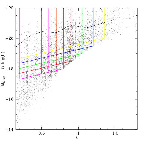
Figure 1: $M_{B}$ for the VVDS galaxies at different redshifts. The solid colored lines denote the various subsamples selected with properties mentioned in Table 1. The dashed line shows the observed evolution in $M_{B}^{*}$.

The VVDS-Deep sample is magnitude limited in the $I_{AB}$ band with $17.5\leq I_{AB}\leq 24$ and covers an area of 0.49 $deg^{2}$ without any color or shape restrictions imposed. The spectroscopic observations were taken with the Visible Multiple-Object Spectrograph (VIMOS, Le Fèvre et al. 2003) at the ESO VLT, whereas the Virmos Deep Imaging survey (VDIS) BVRI photometric data (Le Fèvre et al., 2004) was obtained with the wide field 12k mosaic camera at the CFHT (Canada-France-Hawaii telescope) and is complete and free from surface brightness selection effects (McCracken et al., 2003).

The sample contains 6582 galaxies with secure redshifts, i.e. known at a confidence level $\geq 80\%$. These galaxies have a mean redshift of z $\approx$ 0.83. Fig. 1 shows the absolute magnitude of these galaxies as a function of redshift alongwith the different luminosity-threshold subsamples selected, where the luminosity threshold is assumed to evolve according to the relation $M_{B}(z)=-1.15z+M_{B}(z=0)$. The factor of ’-1.15’ arises from the redshift evolution of the characteristic absolute magnitude, $M_{B}^{*}$, of galaxies as measured in the luminosity function. This value has been determined using the luminosity function measurements obtained within the same sample by Ilbert et al. (2005).

An evolving luminosity threshold needs to be taken into consideration when comparing samples at different epochs, as it provides us with statistically similar samples at different redshifts, having similar evolved luminosities. Assuming that the global evolution of galaxies has as a main consequence to increase the global luminosity of galaxies, we follow the evolution of galaxies with similar properties on average. This falls within the boundaries of standard practice of galaxy evolution studies.

As our subsamples are nearly volume complete, and as we are using all types of galaxies together, we may follow the global increase in the halo mass of an average galaxy. However, we do recognize that this way of selecting galaxies does not garantee to follow the exact same population with cosmic time. Unfortunately, there is no single prescription enabling to tag galaxies and exactly follow their precursors / descendants. Indeed, if this were possible it would be the solution to galaxy evolution. To try to quantify the impact of our selection on the average halo mass, we have used the Millennium simulation. This will be further discussed in the next section.

Samples using a similar type of selection, i.e. using luminosity thresholds, have been extensively studied within a theoretical framework (Zehavi et al., 2005; Coil et al., 2006; Conroy et al., 2006; Zheng et al., 2007). The corresponding HOD parametrisation requires fewer parameters to be fitted as compared to differential, luminosity binned samples. However, this means that one is biased towards increasingly brighter galaxies at higher redshifts, simply due to the fact that the sample is selected in apparent magnitude. As can be seen in Fig. 1, there is a change of about 5 in the B-band absolute magnitude over the redshift bin z $\approx$ [0.1, 1.5]. Table 1 shows the various properties of the subsamples alongwith their number densities. The galaxy number densities were computed by integrating the luminosity functions, derived by Ilbert et al. 2005 on the same galaxy sample and parameterized using Schechter functions. The evolution in the best-fit Schechter parameters, $M^{*}$, $\phi^{*}$ and $\alpha$ was taken into consideration, thereby accounting for luminosity evolution. We estimated the errors on the number densities by propagating the errors on the Schechter parameters. $M_{B}^{thresh}$ denotes the evolving absolute magnitude threshold at the highest redshift. For each $M_{B}^{thresh}$ two samples were obtained, one at low redshift and another at higher redshift with brighter galaxies selected due to the evolving selection cut. The two samples overlap slightly in redshift in order to maximise the number of objects. $M_{B}^{low}$ and $M_{B}^{high}$ are the absolute magnitudes of the evolving cut at the lower and higher redshift limits respectively of the redshift range.

2.2 Studies with simulations

Ideally, we would like to follow statistically the same galaxy population with time in order to study the growth of the underlying dark matter halo mass. This is a tricky issue as it is difficult if not impossible to know the exact progenitors of a descendant galaxy population and how to select them. However, by taking care to follow the exact population mix down to a fixed absolute luminosity, we can minimize the bias in the average halo mass due to the presence/lack of faint or bright galaxies. As mentioned above, this is made possible by accurate measurements of galaxy evolution. In order to tackle this issue we use the Milli-Millennium simulation of galaxies having $270^{3}$ particles in a box of $62.5Mpc/h$ on its side (Springel et al., 2005). The simulations retain information on the progenitor trees of galaxies making it possible to make a comparison with volume-limited samples.

Let us select a galaxy sample at high redshift chosen with a luminosity cut-off in the B-band similar to what is done in the VVDS data, hereafter called the ’parent sample’. This sample is then evolved into two samples at lower redshift, a ’simulated sample’ at the lower redshift, having a luminosity cut-off that is evolved and fainter (again similar to what we did in the data), and another sample that contains all the descendant galaxies at the same lower redshift (hereafter the ’descendant sample’). Doing a galaxy to galaxy match between the two samples would tell us how many galaxies in the simulated data set are actual descendants and therefore the same population followed through time and the effects on the underlying average halo mass. Table 2 shows the Millennium samples selected having roughly the same mean redshift and mean absolute magnitude, $M_{B}$, as in the VVDS data sample of Table 1.

Table 2: Simulated data sets vs. descendants

Sample	$\bar{z}$	$M_{B}^{mean}$	Avg. Halo mass	Overlap $\%$
			$10^{10}M_{\odot}/h$
parent	$0.69$	$-17.86$	$127.04$
simulated	$0.46$	$-17.61$	$164.84$
descendant	$0.46$	$-17.71$	$176.21$	$86.96$
parent	$0.76$	$-18.37$	$135.56$
simulated	$0.51$	$-18.09$	$181.83$
descendant	$0.51$	$-18.17$	$199.49$	$84.03$
parent	$0.90$	$-18.85$	$125.82$
simulated	$0.56$	$-18.50$	$192.06$
descendant	$0.56$	$-18.57$	$219.35$	$82.10$
parent	$0.99$	$-19.32$	$125.60$
simulated	$0.69$	$-18.93$	$177.15$
descendant	$0.69$	$-19.05$	$202.82$	$80.43$
parent	$1.08$	$-19.76$	$126.24$
simulated	$0.69$	$-19.25$	$191.36$
descendant	$0.69$	$-19.42$	$232.73$	$77.12$

We find that at worst 77% of the $M<-20$ and at best 87% of the $M<-18$ simulated luminosity threshold sample are actual descendants at lower redshifts. From Table 2 we can also study the effect of the selections on the underlying average halo mass. It can be seen that typically the underlying halos in the descendant sample are heavier than those in the simulated sample. After taking a closer look at the descendant sample we noted that even though there are a larger number of fainter galaxies, there are also slightly more bright galaxies that lead to a slightly higher average magnitude. The combination of faint satellite galaxies residing in massive halos and fewer galaxies of intermediate luminosity, likely lead to a descendant sample with more massive halos and slightly brighter galaxies on average than the simulated sample. This possibly causes a lower overlap between the simulated and descendant samples for the brightest samples.

The Millennium simulation shows that a growth in halo mass detected in the data would be underestimated with respect to what could be seen ideally. The underestimation in mass is of the order of roughly 10 $\%$, and therefore a measure in the growth of mass of a halo can be mainly attributed to the hierarchical formation of structure and not due to the typology of the selection (taking into consideration the high overlap between the simulated and descendant samples).

2.3 The correlation function

The redshift-space correlation functions for the different luminosity threshold samples have been computed via the Landy & Szalay (1993) estimator:

$$\xi(r_{p},\pi)=\frac{N_{R}(N_{R}-1)}{N_{G}(N_{G}-1)}\frac{GG(r_{p},\pi)}{RR(r_{p},\pi)}-\frac{N_{R}-1}{N_{G}}\frac{GR(r_{p},\pi)}{RR(r_{p},\pi)}+1$$ (1)

where $N_{G}$ and $N_{R}$ are respectively the total number of galaxies and randomly distributed points in the same survey. $GG(r_{p},\pi)$ is the number of distinct galaxy-galaxy pairs with separations lying in the interval ($\pi$,$\pi+d\pi$) in the radial direction and ($r_{p}$,$r_{p}+dr_{p}$) perpendicular to the line of sight. Likewise, $RR(r_{p},\pi)$ and $GR(r_{p},\pi)$ are the number of random-random pairs and galaxy-random pairs respectively in the same interval.

In order to avoid redshift space distortions, $\xi(r_{p},\pi)$ has been integrated along the line of sight to obtain the projected correlation function (Davis & Peebles, 1983):

$$\begin{split}\omega_{p}(r_{p})&=2\int_{0}^{\infty}\xi(r_{p},\pi)\rm{d}\pi\\ &=2\int_{0}^{\infty}\xi\left[\sqrt{r_{p}^{2}+y^{2}}\right]\rm{d}y,\end{split}$$ (2)

where $\xi(r)$ is the real space correlation function with $r$ = $\sqrt{r_{p}^{2}+y^{2}}$. The measurements using the same sample impose a similar upper limit (Pollo et al., 2005, 2006; Meneux et al., 2006). Pollo et al. (2005) found that $\omega_{p}(r_{p})$ is quite insensitive to $\pi_{max}$ in the range of $15Mpc/h<\pi_{max}<25Mpc/h$ for $r_{p}<10Mpc/h$. Too small a value for this limit would cause an underestimation of the small-scale power, and too large a value would introduce noise. After several experiments, the optimal value of $\pi_{max}$=20 Mpc/$h$ has been adopted.

The errors have been estimated using bootstrap resampling of the data, which consists of computing the variance of $w_{p}(r_{p})$ in $N_{real}$ bootstrap realizations of the sample. Each realization is obtained by randomly selecting a subset of galaxies from the data sample allowing for repetitions. A correction factor is then applied to account for the underestimation of the errors obtained using this technique. This correction factor has been calibrated on mock samples to match the ensemble error (accounting for cosmic variance) of the simulated mock samples (see Pollo et al. 2006).

$\begin{array}[]{cc}\includegraphics[width=225.48424pt]{wprp_zfit_mp.ps}&\includegraphics[width=225.48424pt]{wprp_tfit_mp.ps}\\ \end{array}$

Figure 2: The correlation function for the various luminosity threshold samples. The symbols and error bars denote the measurements from the VVDS-Deep. The lines present the best-fit halo model for Z model of Zehavi et al. (2005) in the left panel and for TWZZ model of Tinker et al. (2005) in the right panel.

3 Analytical Modeling

3.1 The Halo model

The analytical model is based on the halo model (see Cooray & Sheth 2002, for a review), here we will briefly mention the main ingredients. All mass is assumed to be bound up into dark matter halos having a range of masses which in turn host galaxies.

In this model the power spectrum, P(k), and/or correlation function, $\xi(r)$, of the galaxies (which are fourier transform pairs) can be written as the sum of two terms. One that dominates on non-linear scales -smaller than the size of a halo, and the other term becoming significant on larger linear scales, known as the 1-halo and 2-halo terms respectively. The 1 halo term arises from pairs of galaxies lying within the same halo, whereas pairs of galaxies lying in different halos contribute to the 2 halo term. In fourier space this can be written as,

$$P(k)=P_{1h}(k)+P_{2h}(k),$$ (3)

where,

$$\begin{split}P_{1h}^{gal}(k,z)&={1\over\bar{n}_{gal}^{2}}\int_{0}^{\infty}dm\,n(m,z)\langle N_{g}(N_{g}-1)|m\rangle\,|u(k|m)|^{2},\\ P_{2h}^{gal}(k,z)&=\left({1\over\bar{n}_{gal}}\int_{0}^{M_{max}}dm\,n(m,z)\langle N_{g}|m\rangle\,b(m,z)\,|u(k|m)|\right)^{2}\\ &\qquad\qquad\times P_{lin}(k,z),\\ \end{split}$$ (4)

and $\bar{n}_{gal}$ is the number density of galaxies:

$$\begin{split}\bar{n}_{gal}=\int_{0}^{\infty}\!dm\,n(m,z)\langle N_{g}|m\rangle.\end{split}$$ (5)

Here, $\langle N_{g}|m\rangle$ is the average number of galaxies occupying a halo of mass $m$, $u(k|m)$ is the halo density profile in fourier space, $n(m,z)$ is the number density of halos of mass $m$, $b(m,z)$ is the bias factor which describes the strength of halo clustering, and $P_{lin}(k,z)$ is the power spectrum of the mass in linear theory all at a given redshift $z$. The upper limit of integration, $M_{max}$, approximately accounts for the halo exclusion effect (different halos cannot overlap) by suppressing the 2-halo term at small scales. Following Zehavi et al. (2004), $M_{max}$ is the mass of the halo with virial radius $r/2$. One can also calculate the one-halo term for the correlation function exactly in real space, which is the approach we have taken. For more details we refer the reader to Berlind & Weinberg (2002). The two-halo term has been computed in k-space and then fourier transformed to obtain the correlation function. Then the projected correlation function is obtained as in Equation 2. Similarly to the data the upper limit is chosen to be finite ($r_{max}$=20 Mpc/$h$) in order to avoid noise caused by uncorrelated distant pairs.

We assume that the density profiles of halos have the form described by Navarro et al. (1997), with a halo concentration parameter $c(M)=11(M/M_{*})^{-0.13}$ to account for the definition of halos as spheres enclosing 200 times the background density (Zehavi et al., 2005) and where $\sigma(M_{*},z)=\delta_{sc}$ ($\sigma$ and $\delta_{sc}$ are defined below). The halo abundances and clustering are described by the Sheth & Tormen (1999) parameterization:

$$\begin{split}\frac{m}{\bar{\rho}}n(m,z){\rm d}m&=f(\nu){\rm d}\nu\\ &=\frac{{\rm d}\nu^{2}}{\nu^{2}}\sqrt{\frac{a\nu^{2}}{2\pi}}exp\left(-\frac{a\nu^{2}}{2}\right)A[1+(a\nu^{2})^{-p}]\\ b(m,z)&=1+\frac{a\nu^{2}-1}{\delta_{sc}}-\frac{2p/\delta_{sc}}{1+(a\nu^{2})^{p}}\\ \nu&=\frac{\delta_{sc}}{\sigma(m,z)},\end{split}$$ (6)

allowing us to write the background density as,

$$\bar{\rho}=\int{\rm d}m\,n(m,z)\,m.$$ (7)

with $\delta_{sc}$ being the critical density required for spherical collapse, extrapolated using linear theory to the present time ($=1.686$, ignoring the weak cosmological dependence), a $\approx$ 0.71, p $=$ 0.3, and A $\approx$ 0.322. $\sigma(m,z)$ is the rms value of the initial fluctuation field when smoothed with a top hat filter and extrapolated to the present time using linear theory.

$$\sigma(m,z)=\sigma(m,0)\frac{G(z)}{G(0)}$$ (8)

where $G$ is the growth factor from Carroll, Press & Turner (1992).

3.2 The HOD models

We will consider two similar HOD models. The first one is based on the model used in Zehavi et al. (2005) (hereafter Z model) to compare to the SDSS data, and is motivated by Kravtsov et al. (2004).

$$\begin{split}\langle N_{g}|m\rangle&=1+\left(\frac{m}{M_{1}}\right)^{\alpha}\qquad\rm{for\,\,m>M_{min}}\\ &=0\qquad\qquad\qquad\rm{otherwise}\end{split}$$ (9)

The second model was proposed by Tinker et al. (2005) (hereafter TWZZ model) and is given by,

$$\begin{split}\langle N_{g}|m\rangle&=1+\frac{m}{M_{1}}\rm{exp}\left(-\frac{M_{cut}}{m}\right)\qquad\rm{for\,\,m>M_{min}}\\ &=0\qquad\qquad\qquad\qquad\qquad\rm{otherwise}\end{split}$$ (10)

where $M_{min}$ is the minimum mass for a halo to host one central galaxy, and $M_{1}$ is the mass of a halo hosting on average one satellite galaxy. The ’1’ represents one central galaxy placed at the center of mass of the parent halo, and the satellite galaxies follow the underlying dark matter distribution. TWZZ model has been used to study the HOD for a range of redshifts and number densities and found to give results for the correlation function in good agreement with various redshift surveys in the range $z=[0-5]$ (Conroy et al., 2006).

Our purpose here will be to obtain the best-fit HOD parameters for the two models, and compare the number-weighted halo masses and number of galaxies. We have decided to use these models in order to keep things simple and easy to interpret. Based on the statistics of the sample and the number of data points used, it is best to use HOD models with a minimal number of free parameters adapted to the science case at hand, i.e. for this paper, the average halo masses and number galaxies mentioned below. The main results that are obtained should remain essentially the same irrespective of the HOD model chosen.

A complementary approach would be to use modeling based on conditional luminosity functions (CLF) or conditional occupation numbers (CON) (e.g. van den Bosch et al. 2003, Yang et al. 2003, Cooray 2006). The present attempt is a first at using a large number of galaxy spectra at high redshift to study the evolutionary behaviour of a few properties pertaining to the galaxy and dark matter distribution. These ’few’ properties are certainly not comprehensive, and this work can be seen as a starting point for more studies using the sample. Moreover, larger data samples from ongoing and upcoming redshift surveys will certainly provide grounds for extensive studies based on CLF/CON.

4 Results

4.1 Results from VVDS

The different parameters were allowed to vary within the following ranges: $10\leq log(M_{min})\leq 15$, $10\leq log(M_{1})\leq 15$, $10\leq log(M_{cut})\leq 15$, $0.5\leq\alpha\leq 2.0$. These limits represent reasonable constraints on the typical mass of a dark matter halo and the power law slope. The minimum mass for a halo to host one central galaxy is usually $\geq 10^{11}h^{-1}M_{\odot}$ for low redshift galaxies (Zehavi et al., 2005), and LBGs at high redshifts (Hamana et al., 2004). At the high mass end, the brightest SDSS galaxy samples have $M_{min}<10^{14}h^{-1}M_{\odot}$. Taking into account our sampling having brightest samples of galaxies at high redshifts, in the hierarchical structure formation scenario this then represents an upper limit on the mass. On the other hand, $M_{1}$ has been found to be $\sim 23M_{min}$ (Zehavi et al., 2005). Furthermore, power law slopes $\geq$ 1.5 are considered “artificially high”, which generally dominate brighter samples that have fewer satellite galaxies on average (Conroy et al., 2006). The number density obtained using Eq. 5 was restricted to lie within 3$\sigma$ from the observed number density given in Table 1. The correlation functions for the different luminosity threshold samples is shown in Fig.2 alongwith the best fits for the two HOD models obtained with the MPFIT algorithm (Markwardt, 2009) that uses the Levenberg-Marquardt technique (Moré et al., 1978) to solve the non-linear least-squares problem using the full covariance matrix.

Table 3: Results for Z model

$M_{B}^{high}$	$log_{10}M_{min}$	$log_{10}M_{1}$	$\alpha$	$log_{10}<M>$	$<N>$	$\chi^{2}/dof$	$\bar{n}_{fit}$
$<-17.77$	$11.05\pm 0.87$	$12.73\pm 1.00$	$0.99\pm 0.10$	$13.00\pm 0.13$	$1.21\pm 0.01$	1.03	37.28
$<-18.00$	$11.21\pm 0.18$	$13.03\pm 0.11$	$1.27\pm 0.08$	$12.97\pm 0.08$	$1.12\pm 0.01$	1.35	26.29
$<-18.27$	$11.37\pm 0.16$	$12.93\pm 0.06$	$1.11\pm 0.12$	$13.14\pm 0.14$	$1.22\pm 0.01$	0.88	20.65
$<-18.50$	$11.63\pm 0.19$	$13.31\pm 0.18$	$1.31\pm 0.09$	$12.98\pm 0.06$	$1.11\pm 0.02$	0.52	11.16
$<-18.71$	$11.88\pm 0.08$	$13.57\pm 0.10$	$1.33\pm 0.16$	$13.10\pm 0.08$	$1.09\pm 0.03$	1.16	6.59
$<-19.00$	$11.76\pm 0.08$	$13.39\pm 0.08$	$1.19\pm 0.24$	$12.88\pm 0.09$	$1.11\pm 0.03$	0.84	8.53
$<-19.16$	$12.06\pm 0.12$	$13.72\pm 0.10$	$1.43\pm 0.27$	$13.11\pm 0.08$	$1.08\pm 0.05$	1.51	4.39
$<-19.50$	$11.92\pm 0.16$	$13.43\pm 0.22$	$1.22\pm 0.25$	$12.94\pm 0.07$	$1.12\pm 0.04$	1.24	5.99
$<-19.48$	$12.06\pm 0.07$	$13.78\pm 0.04$	$1.66\pm 0.18$	$13.13\pm 0.06$	$1.06\pm 0.05$	1.08	4.36
$<-20.00$	$12.35\pm 0.11$	$13.80\pm 0.16$	$1.42\pm 0.41$	$13.09\pm 0.04$	$1.08\pm 0.10$	0.78	2.17

Table 4: Results for TWZZ model

$M_{B}^{high}$	$log_{10}M_{min}$	$log_{10}M_{1}$	$log_{10}M_{cut}$	$log(<M>)$	$<N>$	$\chi^{2}/dof$	$\bar{n}_{fit}$
$<-17.77$	$11.00\pm 0.15$	$12.54\pm 0.39$	$13.01\pm 2.07$	$13.09\pm 0.03$	$1.11\pm 0.01$	1.19	38.00
$<-18.00$	$11.45\pm 0.19$	$11.87\pm 0.71$	$14.93\pm 0.62$	$12.82\pm 0.05$	$1.01\pm 0.02$	1.33	14.51
$<-18.27$	$11.67\pm 0.13$	$13.03\pm 0.22$	$13.32\pm 0.75$	$13.12\pm 0.01$	$1.09\pm 0.02$	0.75	10.06
$<-18.50$	$11.62\pm 0.08$	$12.93\pm 0.08$	$13.26\pm 0.24$	$12.98\pm 0.01$	$1.08\pm 0.02$	0.51	11.09
$<-18.71$	$11.88\pm 0.09$	$13.22\pm 0.29$	$13.45\pm 0.74$	$13.10\pm 0.01$	$1.07\pm 0.04$	1.16	6.40
$<-19.00$	$11.74\pm 0.11$	$13.22\pm 0.15$	$12.62\pm 0.89$	$12.88\pm 0.02$	$1.09\pm 0.03$	0.81	8.71
$<-19.16$	$12.14\pm 0.11$	$13.47\pm 0.19$	$13.49\pm 0.61$	$13.12\pm 0.01$	$1.06\pm 0.06$	1.42	3.67
$<-19.50$	$11.90\pm 0.16$	$13.23\pm 0.35$	$12.73\pm 0.82$	$12.94\pm 0.02$	$1.11\pm 0.04$	1.17	6.18
$<-19.48$	$12.07\pm 0.05$	$13.15\pm 0.16$	$13.97\pm 0.25$	$13.13\pm 0.01$	$1.04\pm 0.05$	0.97	4.18
$<-20.00$	$12.32\pm 0.12$	$13.54\pm 0.45$	$13.21\pm 0.76$	$13.09\pm 0.02$	$1.07\pm 0.10$	0.73	2.27

Tables 3 & 4 show the best-fit parameters for the two different models obtained by a minimum chi-square estimate, the value of the reduced $\chi^{2}$, alongwith the average number-weighted halo masses and number of galaxies per halo defined as:

$$\begin{split}\langle M\rangle&=\frac{\int_{0}^{\infty}n(m)\langle N_{g}|m\rangle m\,\rm{d}m}{\int_{0}^{\infty}n(m)\rm{d}m},\\ \langle N\rangle&=\frac{\int_{0}^{\infty}n(m)\langle N_{g}|m\rangle\rm{d}m}{\int_{0}^{\infty}n(m)\rm{d}m}.\end{split}$$ (11)

The generalized chi-square estimate is obtained the usual way adopting:

$$\chi^{2}=\sum_{i=0}^{n_{bin}}\sum_{j=0}^{n_{bin}}[w_{p}^{obs}(r_{p_{i}})-w_{p}^{model}(r_{p_{i}})]C_{ij}^{-1}[w_{p}^{obs}(r_{p_{j}})-w_{p}^{model}(r_{p_{j}})]$$ (12)

where $n_{\mathrm{bin}}$ is the number of bins and $C_{ij}$ is the covariance of the values of $w_{p}$ between the $i$th and $j$th bins.

The results obtained from both models and given in the tables are found to be in agreement (at least for comparable parameters), which is to be expected as the models are similar. In the case of TWZZ model the power law exponent is kept constant and the number of satellites has a smooth, exponential cut-off. For example, in both cases the value for the minimum mass ($M_{min}$) is very similar if not the same. The power law exponent for the Z model several times shows values of $\alpha$ that are quite high ($>1.4$). Artificially high values have been noticed in fits to simulations as well (Conroy et al., 2006) and occur for galaxy samples at high redshifts. The 1-$\sigma$ error bars on the parameters are obtained with the MPFIT algorithm.

$\begin{array}[]{cc}\includegraphics[width=216.81pt]{mass_growz_mp.eps}&\includegraphics[width=216.81pt]{mass_growt_mp.eps}\\ \end{array}$

Figure 3: The evolution in the number-weighted average halo mass given by Eq.11 for various luminosity threshold samples is shown for the Z model (left panel) and TWZZ model (right panel). The symbols with error bars are obtained from the VVDS, whereas the low redshift symbols at $z=0.1$ with small error bars are from the SDSS. The mass growth can be characterized by $M(z)=M_{0}e^{-\beta z}$, with $\beta=1.07\pm 0.57$ (for the VVDS points), $\beta=1.94\pm 0.10$ (VVDS + SDSS points) in the case of the Z model, and $\beta=1.54\pm 0.13$ (for the VVDS points), $\beta=2.09\pm 0.04$ (VVDS + SDSS points) for the TWZZ model. The values of $\beta$ =0.62 and 2.00 respectively represent the prediction from N-body simulations and the VVDS + SDSS samples.

$\begin{array}[]{cc}\includegraphics[width=216.81pt]{sat_fracz_mp.eps}&\includegraphics[width=216.81pt]{sat_fract_mp.eps}\\ \end{array}$

Figure 4: The evolution in the satellite fraction for various luminosity threshold samples is shown for the Z model (left panel) and TWZZ model (right panel). The symbols with error bars are obtained from the VVDS, whereas the low redshift symbols at $z=0.1$ are from the SDSS. Simply for illustrative purposes, the curves show the reciprocal standard power law behaviour, $y=1/(ax^{b})$, of the data, with $a=13.05$ and $b=0.61$ for the Z model, and $a=20.41$ and $b=0.79$ for the TWZZ model.

Figure 3 shows the number-weighted average halo mass, $<M>$, versus the redshift. The symbols with error bars represent the various sub-samples selected from the VVDS. The error bars are obtained based on error propagation formulas. The point at the lowest redshift ($z\sim 0.1$) is obtained from the SDSS using the best-fit HOD parameters from Zehavi et al. (2005). The mass in this case was calculated using the Z model for the luminosity threshold sample having the same $M-M^{*}$ difference as the samples at higher redshift in the VVDS (where the difference in the r-band for the SDSS has been converted to the B-band, Ilbert et al. 2005). It can be seen that the halo mass evolves and increases as one goes to lower redshifts. This is an indication of the halo mass growth due to the hierarchical aggregation of matter. We find that on average $<M>$ increases by $~{}90\%$ from redshift $\sim 1$ to $\sim 0.5$, showing that massive halos have a rapid accretion phase quite late on, similar to what is expected from N-body simulations (Wechsler et al. 2002). As shown in Wechsler et al. (2002) the mass growth can be easily characterized by the form $M(z)=M_{0}e^{-\beta z}$. The interesting comparison with the addition of low redshift SDSS points gives a linear minimum $\chi^{2}$ fit of $\beta\sim 1.94\pm 0.10$ for the Z Model and $\beta\sim 2.09\pm 0.04$ for the TWZZ model. This is to be compared to the predictions of the mass accretion history of halos in N-body simulations and halos generated through PINOCCHIO (Monaco et al., 2002; Wechsler et al., 2002; Li et al., 2007), where $\beta\sim 0.62$. One can argue that the direct comparison between data obtained from different rest-frame bands can be tricky and could in part lead to a slight boost in $\beta$, even though necessary care has been taken in converting to a common rest-frame band. The latter is reflected in the value obtained for $\beta$, using only the VVDS points leads to a smaller value ($\sim 1.54(1.07)\pm 0.13(0.57)$ for TWZZ (Z) model) albeit with larger error than that obtained from the extrapolation to smaller redshifts, but slightly more consistent with the results from simulations.

For samples at similar redshifts we can see that the number-weighted average halo mass increases with the luminosity threshold of the sample reinforcing the notion that luminous galaxies occupy massive halos. This is in agreement with results obtained from simulations (Conroy et al., 2006) and for LBGs (Ouchi et al., 2005; Lee et al., 2006).

Figure 4 presents the evolution of the galaxy satellite fraction, or the average number of satellite galaxies. The illustrative reciprocal power law behaviour of the dataset shows relatively little change in the satellite fraction (always close to $\sim 0.1$ within 1 $\sigma$) over the redshift range of z=[0.5-1.0]. Over z=[0.1-0.5] there is a sharper increase by a factor $\sim$3 to the local SDSS value of $\sim$0.3. The evolution is mainly accentuated by the SDSS points, although the two lowest redshift VVDS points for the case of the Z model do hint towards an increase with lower redshifts. It is possible that the sharper upturn is once again caused by the complicated comparison between two different data surveys. However, here again care has been taken to convert to the appropriate rest-frame band when making these comparisons and should not affect the overall trend. The increase in the satellite fraction as one goes to lower redshifts can be explained by the dynamical friction of subhalos within their host halos (Conroy et al., 2006). Subhalos are more likely to remain intact within massive halos, whereas in less massive halos they are subject to more dynamical friction and can easily be destroyed. The dynamical friction becomes more/less efficient as a function of the relative masses of subhalos to distinct halos. This is to be compared to recent results obtained by Zheng et al. (2007) who find that the evolution of the satellite fraction follows a trend similar to what is seen here.

The following Fig. 5 shows the evolution in the halo occupation, $N_{g}(m)$, for the extreme luminosity threshold samples obtained from the best fit parameters for the two models. Evidently, the minimum mass, $M_{min}$ increases with the luminosity of the sample as is found locally in the SDSS (Zehavi et al., 2005), again demonstrating that luminous galaxies occupy more massive halos.

$\begin{array}[]{cc}\includegraphics[width=216.81pt]{hod_zmp.ps}&\includegraphics[width=216.81pt]{hod_tmp.ps}\\ \end{array}$

Figure 5: The evolution of the halo occupation for the extreme luminosity threshold samples having $M_{B}<$ -18, -20. The solid line corresponds to the lower redshift sample in each case, and the dashed line to the brighter sample at higher redshift both having the same evolved luminosity threshold (see Table 1). The solid lines correspond to $\bar{z}=0.44,0.67$ and the dashed lines to $\bar{z}=0.66,1.05$ respectively for the samples with $M_{B}<$ -18, -20. The left panel depicts Z model and the right panel TWZZ model.

4.2 Comparison to SDSS

In this section we will compare to results for the same HOD model (Z model) as used in Zehavi et al. (2005). Figure 6 shows the comparison between the masses of halos that have at least one central galaxy ($M_{min}$) and one satellite galaxy ($M_{1}$) on average as a function of $L_{thresh}/L_{*}$, where the ratio is in the B-band, and $L_{thresh}$ is the luminosity threshold given in Table 1 ($L_{thresh}$ and $L_{*}$ are at similar redshifts). Here we will try to compare results obtained at different redshifts. For $40\%$ of the VVDS samples, $M_{min}$ is similar to the local SDSS results within the error bars, with the rest of the VVDS samples having higher values of $M_{min}$. Generally, the VVDS samples exhibit more massive halo masses, $M_{1}$, required to host satellite galaxies than what is seen locally. The value for the power law slope, $\alpha$, is mostly similar to that for local galaxies, with the bright intermediate redshift galaxies showing a higher slope. We can see that generally the samples with higher values for $\alpha$, also have higher values of $M_{1}$ and $M_{min}$ than present-day galaxies.

It is interesting to note the $M_{1}/M_{min}$ ratio, which is on average $\sim$ 45, rather high as compared to the value of $\sim$ 23 for the SDSS galaxies. A direct comparison and interpretation of these results is complicated as one is looking at two different surveys taken in different restframe bands. However, we can speculate that the high value of the ratio implies that the halo with one central galaxy needs to accrete roughly 45 times its mass in order to host a satellite galaxy. In other words, a halo of a given mass is likely to have fewer satellite galaxies at higher redshifts as opposed to a halo of the same mass observed locally.

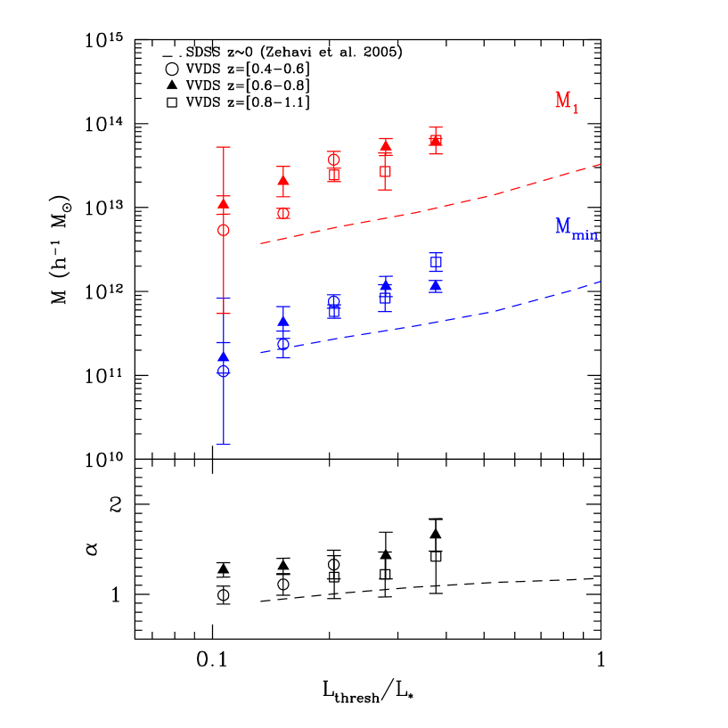
Figure 6: The best fit masses ($M_{min},M_{1}$) and power law slope $\alpha$ of halos for Z model versus $(L_{thresh}/L_{*})$. The different symbols represent results for the VVDS, where each set of symbols correspond to samples lying in different redshift ranges (circles, solid triangles, and empty squares represent samples having $z=[0.4-0.6],[0.6-0.8],[0.8-1.1]$ respectively). The superimposed dashed lines depict the SDSS.

5 Discussion & Conclusions

The comparison of analytical models and data provides useful information of how the distribution of galaxies depends on the underlying dark matter. Subsequently, the best-fitting parameters obtained as a result of this comparison provide physical information regarding the dark matter halos and galaxies.

The size of the VVDS dataset allows one to study, with a unique sample, the global change in the underlying halo properties of an average galaxy down to $z\sim 1$. We attempt to follow the evolution in some properties of a magnitude selected sample, evolving the magnitude cut-off based on accurate measurements of galaxy evolution. We have presented results of the fitting of analytical halo models, incorporating simple HOD models with minimal number of free parameters, to data (in this case the projected 2-point correlation function) from the VVDS survey. This allowed us to study the evolution of the average number weighted halo mass and satellite fraction.

On different scales there are contributions from central-satellite, satellite-satellite, and central-central pairs of galaxies to the correlation function thereby providing constraints on the evolution of the galaxy satellite fraction. The evolution was obtained from data observed in the same restframe band, and provides for simpler interpretations as compared to previous studies using data from different restframe bands. Various luminosity threshold samples at different redshifts were selected and the corresponding best-fit HOD parameters for two similar HOD models obtained. This is done in order to single out possible degeneracies and inconsistencies with the fitting procedure at high redshifts. On the whole, both models are in agreement with each other and show similar trends in evolution. The impact of our selection on the average halo mass is addressed using the Millennium simulation. We find that a growth in halo mass as seen in the data could rather be an underestimation of $\sim 10\%$ to what is seen in an ’ideal’ sample containing all the descendants. Therefore a measure in the growth of mass of a halo can be mainly attributed to the hierarchical formation of structure and not due to the typology of the selection.

We find that the number-weighted average halo mass grows by $\sim 90\%$ from redshift 1.0 to 0.5. This is the first time a growth in the underlying halo mass has been measured at high redshifts within a single data survey, and provides evidence for the rapid accretion phase of massive halos. The mass accretion history follows the form given in Wechsler et al. (2002) with $M(z)=M_{0}e^{-\beta z}$, where $\beta\sim 1.07\pm 0.57(1.54\pm 0.13)$ when only the VVDS points were used and $\beta\sim 1.94\pm 0.10(2.09\pm 0.04)$ after including the SDSS data as reference points at low redshift and depending on the model used to obtain the best fits. The addition of the low redshift SDSS points adds complications due to the addition of possible systematics by comparing data from two different rest-frame bands, even after conversion to a common fiducial band. We adopt the average value of $\beta\sim 1.3\pm 0.30$ from the VVDS points when discussing a growth in halo mass, and found to be slightly higher than the results from N-body simulations.

If we express this result in terms of the expected halo mass at present times, $M_{0}\simeq$ $10^{13.5}h^{-1}M_{\odot}$, such halos appear to accrete $m\sim$ 0.25 $M_{0}$ between redshifts of 0.5 and 1.0. Stewart et al. (2007) have shown that $\sim$ 25% (80%) of $M_{0}=10^{13}h^{-1}M_{\odot}$ halos experienced an $m>0.3M_{0}$ ($m>0.1M_{0}$) merger event in the last 10 Gyr, this would translate into a $m>0.1M_{0}$ merger event over the redshift range z=[0.5-1.0] for the high mass halos here. From merger rate studies one finds that 30% of the stellar mass of massive galaxies with $10^{10}M_{\odot}<M<10^{11}M_{\odot}$ has been assembled through mergers since z=1 (de Ravel et al. 2009, and references therein). The integrated stellar mass growth obtained can then be compared to the halo mass growth obtained here.

For samples at similar redshifts we see that the average halo mass, $<M>$, generally increases with the luminosity threshold of the sample, with a very mild hint of a decreasing galaxy satellite fraction. This implies that galaxies in the faint sample show a stronger probability of being satellites in low mass halos as compared to bright galaxies in massive halos.

We also find that the satellite fraction or average number of satellite galaxies appears to slowly increase over the redshift interval [0.5,1.0], but a stronger increase by a factor of $\sim$3 over z=[0.1,0.5] is seen. This can be understood in terms of the dynamical friction that subhalos hosting satellite galaxies encounter within their host halos. The efficiency of dynamical friction depends on the relative subhalo to halo mass. Subhalos experience more efficient dynamical friction in low mass halos, which can be thought of as progenitor halos at high redshift. The subhalos are continuously subjected to tidal stripping and gravitational heating within the dense environments and get eroded if not completely. As time evolves the halo accretes mass and undergoes mergers with other halos. The subhalos that form as remnants of halo mergers are now more likely to remain intact within the higher mass halo, in turn leading to a larger number of satellite galaxies in present-day halos.

A comparison with the SDSS results shows a few interesting features. The value for $M_{min}$, which is the mass of a halo hosting at least one central galaxy on average, in $40\%$ of the luminosity threshold VVDS samples is similar to values for local SDSS galaxies. Whereas, $M_{1}$ is generally higher for VVDS galaxies as compared to what is seen locally. The ratio of $M_{1}/M_{min}$ is found to be considerably higher (almost a factor of 2) in the VVDS as compared to the SDSS results. This shows that in order to begin hosting satellite galaxies, halos at high redshift need to accrete a larger amount of mass than is seen locally. Hence one would observe roughly twice as many local satellite galaxies than high redshift ones within the same evolved halo mass. This is another line of evidence in favor of the lower observed satellite fraction at high redshift and high local satellite fraction. This interpretation is highly simplified in light of the fact that the results have been obtained with data taken in different restframe bands.

In order to investigate further and better constrain the mass growth and evolution in the number of satellite galaxies per halo over a larger redshift range, one needs to have samples from the same survey at low redshifts. This can be done with samples from deeper and wider redshift surveys. Here we have concentrated on luminosity-threshold samples leading to a link between the luminosity of galaxies and the underlying dark matter distribution. The present paper can be seen as a precursor to many studies that can be carried out with larger samples than the VVDS, including CLF - conditional luminosity function studies (e.g. van den Bosch et al. 2003, etc.), analyses with galaxy samples of different stellar masses (Zheng et al. 2007), etc.. They will certainly add to the understanding of the vast pool of underlying dark matter properties and hopefully obtain tighter constraints on models of galaxy formation.

6 Acknowledgements

UA would like to acknowledge funding from the Marie Curie training network supported by the European Community’s Sixth Framework Programme (FP6). UA also thanks Alessandro Sozzetti and Martin Kilbinger for helpful discussions. The authors thank the anonymous referee for very useful comments and suggestions that helped improve the paper. This research program has been developed within the framework of the VVDS consortium. This work has been funded in part by the ANR program ANR-05-BLAN-0283 and partially supported by the CNRS-INSU and its Programme National de Cosmologie (France), and by the Italian Ministry (MIUR) grants COFIN2000 (MM02037133) and COFIN2003 (No. 2003020150) and by INAF grants (PRIN-INAF 2005) and the grant of Polish Ministry of Science and Higher Education PBZ/MNiSW/07/2006/34. The VLT-VIRMOS observations have been carried out on guaranteed time (GTO) allocated by the European Southern Observatory (ESO) to the VIRMOS consortium, under a contractual agreement between the Centre National de la Recherche Scientifique of France, heading a consortium of French and Italian institutes, and ESO, to design, manufacture and test the VIMOS instrument.

List of Affiliations
¹Laboratoire d’Astrophysique de Marseille, UMR 6110 CNRS-Université de Provence, BP8, F-13376 Marseille Cedex 12, France
²INAF-Osservatorio Astronomico di Brera, Via Brera 28, I-20021, Milan, Italy
³Max Planck Institut für Extraterrestrische Physik (MPE), Giessenbachstrasse 1, D-85748 Garching bei München,Germany
⁴Max Planck Institut für Astrophysik, D-85741, Garching, Germany
⁵Centre de Physique Théorique, UMR 6207 CNRS-Université de Provence, F-13288, Marseille, France
⁶Universitätssternwarte München, Scheinerstrasse 1, D-81679 München, Germany
⁷The Andrzej Soltan Institute for Nuclear Studies, ul. Hoza 69, 00-681 Warszawa, Poland
⁸Astronomical Observatory of the Jagiellonian University, ul Orla 171, PL-30-244, Kraków, Poland
⁹INAF-Osservatorio Astronomico di Bologna, Via Ranzani 1, I-40127, Bologna, Italy
¹⁰IASF-INAF, Via Bassini 15, I-20133, Milano, Italy
¹¹IRA-INAF, Via Gobetti 101, I-40129, Bologna, Italy
¹²INAF-Osservatorio Astronomico di Capodimonte, Via Moiariello 16, I-80131, Napoli, Italy
¹³Università di Bologna, Dipartimento di Astronomia, Via Ranzani 1, I-40127, Bologna, Italy
¹⁴Laboratoire d’Astrophysique de Toulouse/Tabres (UMR5572), CNRS, Université Paul Sabatier - Toulouse III,
Observatoire Midi-Pyrénées, 14 av. E. Belin, F-31400, Toulouse, France
¹⁵Institut d’Astrophysique de Paris, UMR 7095, 98 bis Bvd Arago, F-75014, Paris, France
¹⁶Observatoire de Paris, LERMA, 61 Avenue de l’Observatoire, F-75014, Paris, France
¹⁷Astrophysical Institute Potsdam, An der Sternwarte 16, D-14482, Potsdam, Germany
¹⁸INAF-Osservatorio Astronomico di Roma, Via di Frascati 33, I-00040, Monte Porzio Catone, Italy
¹⁹Universitá di Milano-Bicocca, Dipartimento di Fisica, Piazza delle Scienze 3, I-20126, Milano, Italy
²⁰Integral Science Data Centre, ch. d’Écogia 16, CH-1290, Versoix, Switzerland
²¹Geneva Observatory, ch. des Maillettes 51, CH-1290, Sauverny, Switzerland
²²Centro de Astrofísica da Universidade do Porto, Rua das Estrelas, P-4150-762, Porto, Portugal
²³Institute for Astronomy, 2680 Woodlawn Dr., University of Hawaii, Honolulu, Hawaii, 96822, USA
²⁴School of Physics & Astronomy, University of Nottingham University Park, Nottingham, NG72RD, UK
²⁵Canada France Hawaii Telescope corporation, Mamalahoa Hwy, Kamuela, HI-96743, USA
²⁶INAF - Osservatorio Astronomico di Torino, Strada Osservatorio 20, Pino Torinese, I-10025, Italy

7 Appendix

Here we present the table of values for the projected correlation function ($w_{p}$) and associated errors ($\sigma$) at different values of $r_{p}$ (in units of Mpc $h^{-1}$) for the different subsamples mentioned in Table 1 in the main text. The values for $w_{p}$ and $\sigma$ are reported horizontally at the corresponding values for $r_{p}$ in the top row.

Table 5: Projected correlation function with associated errors at different $r_{p}$ for the different subsamples

$M_{B}^{low}$	$M_{B}^{high}$	0.13	0.25	0.40	0.63	1.00	1.58	2.51	3.98	6.31	10.00	$r_{p}$
$-17.31$	$-17.77$	111.66	82.28	47.85	36.06	27.95	15.88	14.05	10.51	5.96	5.84	$w_{p}$
		37.60	29.03	16.56	10.86	9.12	6.86	5.05	3.48	2.51	2.29	$\sigma$
$-17.66$	$-18.00$	126.04	64.42	39.47	42.53	29.04	23.08	14.54	9.81	6.34	5.50	$w_{p}$
		30.37	19.46	9.63	7.13	5.98	4.16	2.84	2.19	1.70	1.20	$\sigma$
$-17.69$	$-18.27$	144.25	92.38	53.99	50.06	38.30	24.86	19.11	12.79	8.34	7.75	$w_{p}$
		38.60	27.52	14.16	9.26	9.81	6.69	3.95	3.11	2.94	1.80	$\sigma$
$-18.16$	$-18.50$	117.06	74.55	50.91	42.15	29.02	22.90	16.15	12.23	8.27	6.27	$w_{p}$
		30.44	21.94	13.42	6.66	6.67	4.67	3.38	2.72	2.11	1.08	$\sigma$
$-18.02$	$-18.71$	128.23	88.16	49.62	53.91	33.02	27.19	18.93	12.82	8.79	7.89	$w_{p}$
		44.93	25.76	14.40	10.92	8.82	5.67	3.95	2.71	2.65	1.41	$\sigma$
$-18.60$	$-19.00$	102.02	62.36	54.98	29.06	23.63	21.53	14.76	11.98	8.09	6.29	$w_{p}$
		32.39	22.12	13.33	8.43	8.13	5.01	3.70	3.07	2.37	1.23	$\sigma$
$-18.35$	$-19.16$	101.78	99.94	72.26	45.95	32.67	25.17	19.58	14.98	10.30	9.06	$w_{p}$
		39.40	27.35	20.75	9.48	9.99	5.75	4.33	3.53	2.56	1.57	$\sigma$
$-19.04$	$-19.50$	129.74	95.63	68.13	30.44	27.86	21.47	16.47	13.56	10.41	6.53	$w_{p}$
		44.85	30.38	17.90	8.77	8.93	6.04	3.99	3.20	2.39	1.28	$\sigma$
$-18.67$	$-19.48$	98.56	84.77	84.00	55.49	36.81	24.64	21.98	15.27	10.22	8.18	$w_{p}$
		46.76	40.82	25.60	15.59	12.05	7.89	5.94	4.37	3.25	1.95	$\sigma$
$-19.37$	$-20.00$	190.62	118.71	90.48	44.62	37.33	28.48	21.63	16.75	12.71	8.13	$w_{p}$
		73.55	42.16	21.57	12.33	13.63	7.79	5.60	3.70	2.94	1.61	$\sigma$

References

- Benson et al. (2000) Benson A., Cole S., Frenk C.S., Baugh C.M., Lacey C.G., 2000, MNRAS, 311, 793
- Berlind & Weinberg (2002) Berlind A., Weinberg D.H., 2002, ApJ, 575, 587
- Blaizot et al. (2005) Blaizot J., et al., 2005, MNRAS, 360, 159
- Carroll, Press & Turner (1992) Carroll S.M, Press W.H., Turner E.L., 1992, ARA&A, 30, 499
- Coil et al. (2006) Coil A., et al., 2006, ApJ, 644, 671
- Connolly et al. (2002) Connolly A., et al. 2002, ApJ, 579, 42
- Conroy et al. (2006) Conroy C., Wechsler R.H., Kravtsov A.V., 2006, ApJ, 647, 201
- Conroy et al. (2007) Conroy C., et al. 2007, ApJ, 654, 153
- Cooray & Sheth (2002) Cooray A., Sheth R.K., 2002, Phys Reps, 372, 1
- Cooray (2006) Cooray A., 2006, MNRAS, 365, 842
- Davis & Peebles (1983) Davis M., Peebles P.J.E., 1983, ApJ, 267, 465
- de Ravel et al. (2009) de Ravel L. et al., 2009, A&A, 498, 379
- Gott & Turner (1979) Gott J.R., Turner E.L., 1979, ApJ, 232, L79
- Gunn & Gott (1972) Gunn J.E., Gott J.R.III, 1972, ApJ, 176, 1
- Guzzo et al. (1991) Guzzo, L., Iovino, A, Chincarini, G., Giovanelli, R. & Haynes, M.P., 1991, ApJ, 382, L5
- Hamana et al. (2004) Hamana T., Ouchi M., Shimasaku K., Kayo I., Suto Y., 2004, MNRAS, 347, 813
- Hawkins et al. (2003) Hawkins E., Maddox S., Cole S., et al. (the 2dFGRS Team) 2003, MNRAS, 346, 78
- Ilbert et al. (2005) Ilbert O., et al. 2005, A&A, 439, 863
- Jenkins et al. (1998) Jenkins A. et al., 1998, ApJ, 499, 20
- Kauffmann et al. (1999) Kauffmann G., Colberg J.M., Diaferio A., White S.D.M., 1999, MNRAS, 303, 188
- Kravtsov et al. (2004) Kravtsov A.V., Berlind A.A., Wechsler R.H., Klypin A.A., Gottlober S., Allgood B., Primack J.R., 2004, ApJ, 609, 35
- Landy & Szalay (1993) Landy S.D., Szalay A.S., 1993, ApJ, 412, 64
- Le Fèvre et al. (2003) Le Fèvre O., et al., 2003, The Messenger, 111, 18
- Le Fèvre et al. (2004) Le Fèvre O., et al., 2004, A&A, 428, 1043
- Le Fèvre et al. (2005a) Le Fèvre O., et al., 2005, A&A, 439, 845
- Le Fèvre et al. (2005b) Le Fèvre O., et al., 2005, A&A, 439, 877
- Lee et al. (2006) Lee K.-S., Giavalisco M., Gnedin O.Y., Somerville R.S., Ferguson H.C., Dickinson M., Ouchi M., 2006, ApJ, 642, 63
- Li et al. (2007) Li Y., Mo H.J., van den Bosch F.C., Lin W.P., 2007, MNRAS, 379, 689
- Magliocchetti & Porciani (2003) Magliocchetti M., Porciani C., 2003, MNRAS, 346, 186
- Markwardt (2009) Markwardt C., 2009, ASPC, 411, 251
- McCracken et al. (2003) Mc Cracken H., et al., 2003, A&A, 410, 17
- Meneux et al. (2006) Meneux B., et al. 2006, A&A, 452, 387
- Monaco et al. (2002) Monaco P., Theuns T., Taffoni G, 2002, MNRAS, 331, 587
- Moré et al. (1978) Moré J., Numerical Analysis, ed. G. A. Watson (Springer-Verlag: Berlin), 630, 105
- Navarro et al. (1997) Navarro J., Frenk C., White S.D.M., 1997, ApJ, 490, 493
- Ouchi et al. (2005) Ouchi M., Hamana T., Shimasaku K., et al. 2005, ApJL, 635, 117
- Peacock (1997) Peacock J.A., 1997, MNRAS, 284, 885
- Peebles (1974) Peebles P.J.E., 1974, A&A, 32, 197
- Phleps et al. (2006) Phleps S., Peacock J.A., Meisenheimer K., Wolf C., 2006, A & A, 457, 145
- Pollo et al. (2005) Pollo A. et al., 2005, A& A, 439, 887
- Pollo et al. (2006) Pollo A. et al., 2006, A& A, 451, 409
- Press et al. (1992) Press W.H., Teukolsky S.A., Vetterling W.T., Flannery B.P., 1992, Numerical Recipes in C, Cambridge University Press
- Sheth & Tormen (1999) Sheth R.K., Tormen G., 1999, MNRAS, 308, 119
- Springel et al. (2005) Springel V., 2005, Nature, 435, 629
- Stewart et al. (2007) Stewart K., Bullock J.S., Wechsler R.H., Maller A.H., Zentner A.R., 2007, astro-ph/0711.5027
- Tinker et al. (2005) Tinker J.L., Weinberg D.H., Zheng Z., Zehavi I., 2005, ApJ, 631, 41
- Totsuji & Kihara (1969) Totsuji H., Kihara T., 1969, PASJ, 21, 221
- van den Bosch et al. (2003) van den Bosch F.C., Yang X., Mo H.J., 2003, MNRAS, 340, 771
- Wechsler et al. (2002) Wechsler R.H., Bullock J.S., Primack J.R., Kravtsov A.V., Dekel A., 2002, ApJ, 568, 52
- Weinberg et al. (2004) Weinberg D.H., Davé R., Katz N., Hernquist L., 2004, ApJ, 601, 1
- White & Rees (1978) White S.D.M., Rees M.J., 1978, MNRAS, 183, 341
- Yang et al. (2003) Yang X., Mo H.J., van den Bosch F.C., 2003, MNRAS, 339, 1057
- Zehavi et al. (2004) Zehavi I., Weinberg D.H., Zheng Z., et al. 2004, ApJ, 608, 16
- Zehavi et al. (2005) Zehavi I., et al., 2005, ApJ, 630, 1
- Zheng (2004) Zheng Z., 2004, ApJ, 610, 61
- Zheng et al. (2007) Zheng Z., Coil A., Zehavi I., 2007, ApJ, 667, 760