Object-image correspondence for curves under finite and affine cameras

Abstract.

We provide criteria for deciding whether a given planar curve is an image of a given spatial curve, obtained by a central or a parallel projection with unknown parameters. These criteria reduce the projection problem to a certain modification of the equivalence problem of planar curves under affine and projective transformations. The latter problem can be addressed using Cartan’s moving frame method. This leads to a novel algorithmic solution of the projection problem for curves. The computational advantage of the algorithms presented here, in comparison to algorithms based on a straightforward solution, lies in a significant reduction of a number of real parameters that has to be eliminated in order to establish existence or non-existence of a projection that maps a given spatial curve to a given planar curve. The same approach can be used to decide whether a given finite set of ordered points on a plane is an image of a given finite set of ordered points in $\mathbb{R}^{3}$. The motivation comes from the problem of establishing a correspondence between an object and an image, taken by a camera with unknown position and parameters.

Keywords: Curve matching, central and parallel projections, finite projective and affine cameras, geometric invariants

1. Introduction

The problem of identification of objects in 3D with their planar images, taken by a camera with unknown position and parameters, is an important task in computer object recognition. Since the defining features of many objects can be represented by curves, obtaining an algorithmic solution for the projection problem for curves is essential, but appears to be unknown in the case of projections with a large number of free parameters. We address this problem for two classes of cameras: finite projective cameras and affine cameras.

The set of finite projective cameras (also called finite cameras) has 11 parameters and corresponds to the set of central projections. The set of affine cameras has 8 parameters and corresponds to the set of parallel projections. An affine camera can be obtained as a limit of a finite camera, as the camera center approaches infinity along the perpendicular from the camera center to the image plane. See [hartley04] for an overview of camera projections and related geometry. An affine camera has fewer parameters and provides a good approximation of a finite camera when the distance between a camera and an object is significantly greater than the object depth [hartley04, stiller06].

The projection problem for curves is formulated as follows:

Problem 1.

Given a curve ${\mathcal{Z}}$ in $\mathbb{R}^{3}$ and a curve ${\mathcal{X}}$ in $\mathbb{R}^{2}$, does there exist a finite camera (central projection) or an affine camera (parallel projection) that maps ${\mathcal{Z}}$ to ${\mathcal{X}}$?

A straightforward approach to Problem 1, in the case of central projections, leads to the following real quantifier eliminations problem:

Problem 2.

Given a curve ${\mathcal{Z}}$ in $\mathbb{R}^{3}$ and a curve ${\mathcal{X}}$ in $\mathbb{R}^{2}$ decide whether there exist 11 real parameters, which describe a central projection $P$, such that

$$\forall x\in{\mathcal{X}}\,\,\exists z\in{\mathcal{Z}},\mbox{ such that }x=P(z)?$$

Real quantifier elimination problems are algorithmically solvable [tarski:51]. There is an extensive body of literature devoted to computationally effective methods in real quantifier elimination, including [Collins:75], [Grig88], [Hong:90a], [HRS93], [pedersen93]. High computational complexity of these algorithms make a reduction in the number of quantifiers to be desirable.

The projection criteria, developed in this paper, reduces the projection problem to the problem of deciding whether the given planar curve ${\mathcal{X}}$ is equivalent to a curve in a certain family of planar curves under an action of the projective group, in the case of central projections, and under the action of the affine group in the case of parallel projections. The family of curves depends on 3 parameters in the case of central projections, and on 2 parameters in the case of parallel projections.

The group-equivalence problem can be solved by an adaptation Cartan’s moving frame method. Following this method for the case of central projections, when ${\mathcal{Z}}$ and ${\mathcal{X}}$ are rational algebraic curves, we define two corresponding rational signature maps ${\mathcal{S}}_{\mathcal{X}}\colon\mathbb{R}\to\mathbb{R}^{2}$ and ${\mathcal{S}}_{\mathcal{Z}}\colon\mathbb{R}^{4}\to\mathbb{R}^{2}$. Construction of these signature maps requires only differentiation and arithmetic operations and is computationally trivial. Problem 2 reduces to

Problem 3.

Given two rational maps ${\mathcal{S}}_{\mathcal{X}},\,\mathbb{R}\to\mathbb{R}^{2}$ and ${\mathcal{S}}_{\mathcal{Z}}\colon\mathbb{R}^{4}\to\mathbb{R}^{2}$ decide whether there exist $c_{1},c_{2},c_{3}\in\mathbb{R}$, such that

$$\forall t\in\mathbb{R},\,\mbox{ where }{\mathcal{S}}_{\mathcal{X}}(t)\mbox{ is defined},\,\exists s\in\mathbb{R},\mbox{ such that }{\mathcal{S}}_{\mathcal{X}}(t)={\mathcal{S}}_{\mathcal{Z}}(s,c_{1},c_{2},c_{3}).$$

Thus, the projection criteria developed in this paper allows us to reduce the number of real quantifiers that need to be eliminated from 13 (11 parameters define a central projection, one is needed to parametrize curve ${\mathcal{Z}}$ and another one to parametrize curve ${\mathcal{X}}$) to 5. The case of parallel projection is treated in the similar manner and leads to the reduction of the number of real quantifiers that need to be eliminated from 10 to 4.

Previous works on related problems include [feldmar95], where a solution to Problem 1 is given for finite cameras with known internal parameters. In this case, the number of free parameters is reduced from 11 to 6 parameters, representing the position and the orientation of the camera. The method presented in [feldmar95] also uses an additional assumption that a planar curve ${\mathcal{X}}\subset\mathbb{R}^{2}$ has at least two points, whose tangent lines coincide. In the current paper we do not assume that the internal camera parameters are known.

A solution of the projection problem for finite ordered sets of points under affine cameras appeared in [stiller06, stiller07] and served as an inspiration for this paper. In Section 7, we summarize the approach of [stiller06, stiller07] and indicate how the solution of Problem 1 may be adapted to produce an alternative solution to the projection problem for finite ordered sets of points under either affine or finite cameras.

One of the advantages of the novel approach to the solution of Problem 1, introduced in this paper, is its universality: essentially the same method can be adapted to various types of the projections and various types of objects, both continuous and discrete. Similar to many previous considerations of the projection problems, we utilize actions of affine and projective groups to obtain a solution to the projection problem. Our literature search did not yield, however, neither previous solutions for the projection problem for curves, where cameras with unknown internal and external parameters are considered, nor a similar combination of ideas as presented here. The algorithmic solution presented here, would have to be fine-tuned to become practically useful in real-life applications, but we believe, it has a good potential to develop into a practically efficient method. Some directions of such improvement are indicated in Section 8 of the paper.

Problem 1 can be generalized to higher dimensions as follows:

Problem 4.

Given a curve ${\mathcal{Z}}$ in $\mathbb{R}^{n}$ and a curve ${\mathcal{X}}$ in $\mathbb{R}^{n-1}$ ($n\geq 3)$ does there exist a central or a parallel projection from $\mathbb{R}^{n+1}$ to a hyperplane in $\mathbb{R}^{n}$ that maps ${\mathcal{Z}}$ to ${\mathcal{X}}$?

The solution, proposed in this paper, has a straightforward adaptation to higher dimensions and will result in a reduction in the number of quantifiers that need to be eliminated from $n(n+1)+1$ to $n+2$ for central projections and from $n^{2}+1$ to $n+1$ for parallel projections. In this paper, we restrict the presentation to the case of $n=3$, which has applications in computer image recognition and presents least computational challenge.

The paper is structured as follows. After reviewing the geometry of finite and affine cameras in Section 2, we define actions of direct products of affine and projective groups on the set of cameras in Section 3. We use these actions to reduce Problem 1 for finite and affine projections to a modification of the equivalence problem for planar curves under projective and affine transformations, respectively. This leads to the main result of this paper, projection criteria for curves, formulated in Section 4. In Section 5, we review a solution for the group-equivalence problem, based on differential signature construction [calabi98]. In Section 6, we combine our projection criteria and the differential signature construction in order to obtain an algorithm for solving the projection problem and show some examples. Although the projection criteria derived in Section 4 of the paper are valid for arbitrary classes of curves (and, more generally, for arbitrary subsets of $\mathbb{R}^{3}$ and $\mathbb{R}^{2}$, respectively) the computational algorithms of Section 6 are developed for rational algebraic curves. We will consider a possible generalization of these algorithms to non-rational algebraic curves in an upcoming paper [bk-prep]. In Section 7 we indicate how the approach of this paper can be applied to the projection problem for finite ordered sets of points. A solution to the latter problem for affine projections appeared in [stiller06, stiller07]. We provide a brief comparison of the two approaches. In Section 8, we discuss possible variations of our algorithm based on alternative solutions of the group-equivalence problem, as well as possible adaptations to curves presented by samples of discrete points whose coordinates may be known only approximately.

2. Finite and affine cameras

A simple pinhole camera is shown in Figure 1 and corresponds to a central projection.

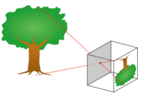
Figure 1. Pinhole camera [pinhole-figure].

Let $(z_{1},z_{2},z_{3})$ be coordinates in $\mathbb{R}^{3}$, relative to an orthonormal coordinate basis, such that the camera is located at the origin on $\mathbb{R}^{3}$ and the image plane is passing through the point $(0,0,1)$ perpendicular to the $z_{3}$-axis. We assume that a coordinate system on the image plane is provided by the first two coordinate functions on $\mathbb{R}^{3}$, i.e. $x(z_{1},z_{2},1)=z_{1}$ and $y(z_{1},z_{2},1)=z_{2}$. Then a point $(z_{1},z_{2},z_{3})$, such that $z_{3}\neq 0$ is projected to the point

(1) $$(x,y)=\left(\frac{z_{1}}{z_{3}},\frac{z_{2}}{z_{3}}\right).$$

We introduce a freedom to choose the position of the camera center ($3$ degrees of freedom), the position of the image plane, ($3$ degrees of freedom), as well as a choice of, in general, non-orthogonal, linear system of coordinates on the image plane ($5$ degrees of freedom, since the overall scale is absorbed by the previous choices, i.e., the choice of the distance between the image plane and the camera center). For real parameters $p_{ij},i=1\dots 3,j=1\dots 4$, a generic projection maps a point $(z_{1},z_{2},z_{3})\in\mathbb{R}^{3}$ to a point in the image plane with coordinates

(2) $$x = \frac{p_{11}\,z_{1}+p_{12}\,z_{2}+p_{13}\,z_{3}+p_{14}}{p_{31}\,z_{1}+p_{32}\,z_{2}+p_{33}\,z_{3}+p_{34}},$$

$$y = \frac{p_{21}\,z_{1}+p_{22}\,z_{2}+p_{23}\,z_{3}+p_{24}}{p_{31}\,z_{1}+p_{32}\,z_{2}+p_{33}\,z_{3}+p_{34}}.$$

A convenient matrix representation of this map is obtained by embedding $\mathbb{R}^{n}$ into projective space $\mathbb{P}^{n}$ and utilizing homogeneous coordinates on $\mathbb{P}^{n}$.

Notation 5.

Square brackets around matrices (and, in particular, vectors) will be used to denote an equivalence class with respect to multiplication of a matrix by a nonzero scalar. Multiplication of equivalence classes of matrices $A$ and $B$ of appropriate sizes is well-defined by $[A]\,[B]:=[A\,B]$.

With this notation a point $(x,y)\in\mathbb{R}^{2}$ corresponds to a point $[x,y,1]=[\lambda x,\lambda y,\lambda]\in\mathbb{P}^{2}$ for all $\lambda\neq 0$, and a point $(z_{1},z_{2},z_{3})\in\mathbb{R}^{3}$ corresponds to $[z_{1},z_{2},z_{3},1]\in\mathbb{P}^{3}$. We will refer to the points in $\mathbb{P}^{n}$ whose last homogeneous coordinate is zero as points at infinity. In homogeneous coordinates projection (2) is given by

(3) $$[x,\,y\,,1]^{\operatorname{tr}}=[P]\,[z_{1},\,z_{2},\,z_{3},\,1]^{\operatorname{tr}},$$

where $P$ is $3\times 4$ matrix of rank 3.

Matrix $P$ has a $1$-dimensional kernel, i. e. there exists a non-zero point $(z^{0}_{1},z^{0}_{2},z^{0}_{3},z^{0}_{4})\in\mathbb{R}^{4}$ such that $P\,(z^{0}_{1},z^{0}_{2},z^{0}_{3},z^{0}_{4})^{tr}=(0,0,0)^{tr}$. Therefore, the image of the point $[z^{0}_{1},z^{0}_{2},z^{0}_{3},z^{0}_{4}]\in\mathbb{P}^{3}$ under the projection is undefined (recall that $[0,0,0]$ is not a point in $\mathbb{P}^{2}$). Geometrically the kernel of $P$ corresponds to the center of the projection.

Camera is called finite if its center is not at infinity. In the case of finite cameras the left $3\times 3$ submatrix of $P$ is non-singular.

On the contrary an infinite camera has its center at an infinite point of $\mathbb{P}^{3}$ and so the left $3\times 3$ submatrix of $P$ is singular. An infinite camera is called affine when the preimage of the line at infinity in $\mathbb{P}^{2}$ is the plane at infinity in $\mathbb{P}^{3}$. In this case $[P]$ can be represented by a matrix whose last row is $(0,0,0,1)$. Affine cameras correspond to parallel projections from $\mathbb{R}^{3}$ to a plane. Eight degrees of freedom reflect a choice of the direction of a projection and a choice of, in general non-orthogonal, linear system of coordinates on the image plane. An image plane may be assumed to be perpendicular to the direction of the projection, since other choices are absorbed in the freedom to choose a coordinate system on the image plane.

Definition 6.

A set of equivalence classes $[P]$, where $P=(p_{ij})^{i=1\dots 3}_{j=1\dots 4}$ is a $3\times 4$ matrix whose left $3\times 3$ submatrix is non-singular, is called the set of finite projections and is denoted ${\mathcal{FP}}$.

A set of equivalence classes $[P]$, where $P=(p_{ij})^{i=1\dots 3}_{j=1\dots 4}$ has rank 3 and its last row is $(0,0,0,\lambda)$, $\lambda\neq 0$, is called the set of affine projections and is denoted ${\mathcal{AP}}$. Affine projections are also called generalized weak perspective projections [stiller06, stiller07]).

Equation (2) determines a central projection $\mathbb{R}^{3}\to\mathbb{R}^{2}$ when $[P]\in{\mathcal{FP}}$ and it determines a parallel projection when $[P]\in{\mathcal{AP}}$.

The sets of finite and affine projections are disjoint. Projections that are not included in these two classes are infinite non-affine projections. These are not frequently used in computer vision and are not considered in this paper.

A simple pinhole camera projection (1) is represented by the matrix:

(4) $${P_{f}^{0}}:=\left[\begin{array}[]{cccc}1&0&0&0\\ 0&1&0&0\\ 0&0&1&0\end{array}\right]$$

and is called the standard finite projection. The standard affine projection is the orthogonal projection on the $z_{1}z_{2}$-plane. It is represented by the matrix

(5) $${P_{a}^{0}}:=\left[\begin{array}[]{cccc}1&0&0&0\\ 0&1&0&0\\ 0&0&0&1\end{array}\right].$$

3. Group actions

Since group actions and, in particular, actions of the affine and projective groups play a crucial role in our construction, we review here the relevant definitions:

Definition 7.

An action of a group $G$ on a set ${S}$ is a map ${\Phi}\colon G\times{S}\to{S}$ that satisfies the following two properties:

1. ${\Phi}(e,s)=s$, $\forall s\in{S}$, where $e$ is the identity of the group.

2. ${\Phi}(g_{1},{\Phi}(g_{2},s))={\Phi}(g_{1}\,g_{2},s)$, $\forall\,s\in{S}$ and $\forall\,g_{1},g_{2}\in G$.

For $g\in G$ and $s\in{S}$ we sometimes write ${\Phi}(g,s)=g\,s.$

Definition 8.

An action is called transitive if for all $s_{1},s_{2}\in{S}$ there exists $g\in G$ such that $s_{1}=g\,s_{2}$.

Definition 9.

For a fixed element $s\in{S}$ the set $G_{s}=\{g\in G|gs=s\}\subset G$ is called the stabilizer of $s$.

It can be shown that a stabilizer $G_{s}$ is a subgroup of $G$.

Definition 10.

The projective group ${\mathcal{PGL}}(n+1)$ is a quotient of the general linear group ${{\mathcal{G}L}}(n+1)$, consisting of $(n+1)\times(n+1)$ non-singular matrices, by a 1-dimensional abelian subgroup $\lambda I$, where $\lambda\neq 0\in\mathbb{R}$ and $I$ is the identity matrix. Elements of ${\mathcal{PGL}}(n+1)$ are equivalence classes $[B]=[\lambda B]$, where $\lambda\neq 0$ and $B\in{{\mathcal{G}L}}(n+1)$.

The affine group ${\mathcal{A}}(n)$ is a subgroup of ${\mathcal{PGL}}(n+1)$ whose elements $[B]$ have a representative $B\in{{\mathcal{G}L}}(n+1)$ whose last row is $(0,\dots,0,1)$.

The special affine group ${\mathcal{SA}}(n)$ is a subgroup of ${\mathcal{A}}(n)$ whose elements $[B]$ have a representative $B\in{{\mathcal{G}L}}(n+1)$ with determinant $1$ and the last row equal to $(0,\dots,0,1)$.

In homogeneous coordinates the standard action of the projective group ${\mathcal{PGL}}(n+1)$ on $\mathbb{P}^{n}$ is defined by:

(6) $${\Phi}([B],[z_{1},\dots,z_{n},z_{0}]^{\operatorname{tr}})=[B]\,[z_{1},\dots,z_{n},z_{0}]^{\operatorname{tr}}.$$

The action (6) induces almost everywhere defined linear-fractional action of ${\mathcal{PGL}}(n+1)$ on $\mathbb{R}^{n}$. In particular, for $n=2$, $[B]\in{\mathcal{PGL}}(3)$ we have

(7) $$(x,y)\to\left(\frac{b_{11}\,x+b_{12}\,y+b_{13}}{b_{31}\,x+b_{32}\,y+b_{33}},\frac{b_{21}\,x+b_{22}\,y+b_{23}}{b_{31}\,x+b_{32}\,y+b_{33}}\right).$$

The restriction of (6) to ${\mathcal{A}}(n)$ induces an action on $\mathbb{R}^{n}$ consisting of compositions of linear transformations and translations. In particular, for $n=2$ and $[B]\in{\mathcal{A}}(2)$ represented by a matrix $B$ whose last row is $(0,0,0,1)$

(8) $$(x,y)\to\left(b_{11}\,x+b_{12}\,y+b_{13},\,b_{21}\,x+b_{22}\,y+b_{23}\right).$$

3.1. Action on finite cameras

A straightforward exercise in matrix multiplication shows that the map ${\Phi}:\left({{\mathcal{PGL}}(3)}\times{\mathcal{A}(3)}\right)\times{\mathcal{FP}}\to{\mathcal{FP}}$ defined by

(9) $${\Phi}\big{(}([A],[B]),\,[P])=[A]\,[P]\,[B^{-1}]$$

for $[P]\in{\mathcal{FP}}$ and $([A],[B])\in{{\mathcal{PGL}}(3)}\times{\mathcal{A}(3)}$, satisfies Definition 7 of a group-action.

Proposition 11.

The action of ${{\mathcal{PGL}}(3)}\times{\mathcal{A}(3)}$ on ${\mathcal{FP}}$, defined by (9) is transitive.

Proof.

According to Definition 8 we need to prove that for all $[P_{1}],[P_{2}]\in{\mathcal{FP}}$ there exists $([A],[B])\in{{\mathcal{PGL}}(3)}\times{\mathcal{A}(3)}$ such that $[A][P_{1}][B^{-1}]=[P_{2}]$. It is sufficient to prove that for all $[P]\in{\mathcal{FP}}$ there exists $([A],[B])\in{{\mathcal{PGL}}(3)}\times{\mathcal{A}(3)}$ such that $[P]=[A]\,[{P_{f}^{0}}]\,[B]$, where $[{P_{f}^{0}}]$ is the standard finite projection (4). A finite projection is given by a $3\times 4$ matrix $P=(p_{ij})^{i=1\dots 3}_{j=1\dots 4}$ whose left $3\times 3$ submatrix is non-singular. Therefore there exist $c_{1},\,c_{2},\,c_{3}\in\mathbb{R}$ such that $p_{*4}=c_{1}\,p_{*1}+c_{2}\,p_{*2}+c_{3}\,p_{*3}$, where $p_{*j}$ denotes the $j$-th column of the matrix $P$. We define $A:=(p_{ij})^{i=1\dots 3}_{j=1\dots 3}$ to be the left $3\times 3$ submatrix of $P$ and

(10) $$B:=\left(\begin{array}[]{cccc}1&0&0&c_{1}\\ 0&1&0&c_{2}\\ 0&0&1&c_{3}\\ 0&0&0&1\end{array}\right).$$

We observe that $([A],[B])\in{{\mathcal{PGL}}(3)}\times{\mathcal{A}(3)}$ and $[A][{P_{f}^{0}}][B]=[P]$. ∎

Corollary 12.

The set ${\mathcal{FP}}$ of finite projections is diffeomorphic to the homogeneous space $({{\mathcal{PGL}}(3)}\times{\mathcal{A}(3)})/H_{f}^{0}$, where $H_{f}^{0}$ is the 9-dimensional stabilizer of $[{P_{f}^{0}}]$.

A straightforward computation shows that

(11) $$H_{f}^{0}=\left\{\left([A],\,\left[\begin{array}[]{cc}A&\bf{0}^{\operatorname{tr}}\\ \bf{0}&1\end{array}\right]\right)\right\},\mbox{ where $A\in{{\mathcal{G}L}}(3)$.}$$

Remark 13.

It follows from the proof of Proposition 11 that any finite projection is a composition of a translation in $\mathbb{R}^{3}$ (corresponding to translation of the camera center to the origin), the standard projection (4) (pinhole camera), and a projective transformation on the image plane.

3.2. Action on affine cameras

Formula (9) with $[P]\in{\mathcal{AP}}$ and $([A],[B])\in{\mathcal{A}(2)}\times{\mathcal{A}(3)}$ defines an action of the direct product ${\mathcal{A}(2)}\times{\mathcal{A}(3)}$ on the set of affine projections ${\mathcal{AP}}$.

Proposition 14.

The action of ${\mathcal{A}(2)}\times{\mathcal{A}(3)}$ on ${\mathcal{AP}}$, defined by (9), is transitive.

Proof.

It is sufficient to prove that for all $[P]\in{\mathcal{AP}}$ there exists $([A],[B])\in{\mathcal{A}(2)}\times{\mathcal{A}(3)}$ such that $[P]=[A]\,[{P_{a}^{0}}]\,[B]$, where ${P_{a}^{0}}$ is the standard projection (5). An affine projection $P$ is given by the matrix

(12) $$P=\left(\begin{array}[]{cccc}p_{11}&p_{12}&p_{13}&p_{14}\\ p_{21}&p_{22}&p_{23}&p_{24}\\ 0&0&0&1\end{array}\right)$$

of rank 3. Therefore there exist $1\leq i<j\leq 3$ such that the rank of the submatrix $\left(\begin{array}[]{cc}p_{1i}&p_{1j}\\ p_{2i}&p_{2j}\end{array}\right)$ is 2. Then for $1\leq k\leq 3$, such that $k\neq i$ and $k\neq j$, there exist $c_{1},\,c_{2}\in\mathbb{R}$, such that $\left(\begin{array}[]{c}p_{1k}\\ p_{2k}\end{array}\right)=c_{1}\,\left(\begin{array}[]{c}p_{1i}\\ p_{2i}\end{array}\right)+c_{2}\,\left(\begin{array}[]{c}p_{1j}\\ p_{2j}\end{array}\right)$. We define

(13) $$A:=\left(\begin{array}[]{ccc}p_{1i}&p_{1j}&p_{14}\\ p_{2i}&p_{2j}&p_{24}\\ 0&0&1\end{array}\right)$$

and define $B$ to be the matrix whose columns are vectors $b_{*i}:=(1,0,0,0)^{\operatorname{tr}}$, $b_{*j}:=(0,1,0,0)^{\operatorname{tr}}$, $b_{*k}:=(c_{1},c_{2},1,0)^{\operatorname{tr}}$, $b_{*4}=(0,0,0,1)^{\operatorname{tr}}$. We observe that $([A],[B])\in{\mathcal{A}(2)}\times{\mathcal{A}(3)}$ and that $[A][{P_{a}^{0}}][B]=[{P_{a}^{0}}]$. ∎

Remark 15.

Note that there are only three possible values of $(i,j,k)$ in the above proof:

1. $(i,\,j,\,k)=(1,2,3)$, then

   (14) $$B=\left(\begin{array}[]{cccc}1&0&c_{1}&0\\ 0&1&c_{2}&0\\ 0&0&1&0\\ 0&0&0&1\end{array}\right);$$

2. $(i,\,j,\,k)=(1,3,2)$, then the corresponding $B$ is obtained by interchanging the second and the third column in (14);

3. $(i,\,j,\,k)=(2,3,1)$, then the corresponding $B$ is obtained by a cyclic shift (by one to the right) of the first three columns in (14).

Corollary 16.

The set ${\mathcal{AP}}$ of affine projections is diffeomorphic to the homogeneous space $({\mathcal{A}(2)}\times{\mathcal{A}(3)})/H_{a}^{0}$, where $H_{a}^{0}$ is the 10-dimensional stabilizer of $[{P_{a}^{0}}]$.

A straightforward computation shows that

(15) $$H^{0}_{a}=\left\{\left(\left[\begin{array}[]{cccc}m_{11}&m_{12}&a_{1}\\ m_{21}&m_{22}&a_{2}\\ 0&0&1\end{array}\right],\left[\begin{array}[]{cccc}m_{11}&m_{12}&0&a_{1}\\ m_{21}&m_{22}&0&a_{2}\\ m_{31}&m_{32}&m_{33}&a_{3}\\ 0&0&0&1\end{array}\right]\right)\right\},$$

where $m_{33}\,(m_{11}m_{22}-m_{12}m_{21})\neq 0$.

4. Projection criteria for curves

In this section we formulate criteria for the existence of a finite or an affine projection that maps a given algebraic curve in $\mathbb{R}^{3}$ to a given algebraic curve in $\mathbb{R}^{2}$.

We recall [fulton] that for every algebraic curve ${\mathcal{X}}\subset\mathbb{R}^{n}$ there exists a unique projective algebraic curve $[{\mathcal{X}}]\subset\mathbb{P}^{n}$ such that $[{\mathcal{X}}]$ is the smallest projective variety containing ${\mathcal{X}}$. As before, we identify a point on $[{\mathcal{X}}]$ with the column vector of its homogeneous coordinates.

Definition 17.

We say that a curve ${\mathcal{Z}}\subset\mathbb{R}^{3}$ projects onto ${\mathcal{X}}\subset\mathbb{R}^{2}$ if there exists a $3\times 4$ matrix $P$ of rank 3 such that the set $[P][{\mathcal{Z}}]$ is dense in $[{\mathcal{X}}]$. In this definition, we allow the center of the projection $[P]$ to lie on $[{\mathcal{Z}}]$, and if this happens $[P][{\mathcal{Z}}]$ is undefined at one point.

Note that if ${\mathcal{Z}}\subset\mathbb{R}^{3}$ projects onto ${\mathcal{X}}\subset\mathbb{R}^{2}$ according to Definition 17 then the image of ${\mathcal{Z}}$ under the map (2) is dense in ${\mathcal{X}}$. Disregarding possible exclusions of finites sets of points, we write ${\mathcal{X}}=[P]({\mathcal{Z}})$ and $[{\mathcal{X}}]=[P][{\mathcal{Z}}]$ if Definition 17 is satisfied.

In the next two subsections we show that the projection problem for central and parallel projections can be reduced to a variation of the equivalence problem of planar curves under projective and affine actions, respectively.

Definition 18.

We say that two curves ${\mathcal{X}}_{1}\subset\mathbb{R}^{n}$ and ${\mathcal{X}}_{2}\subset\mathbb{R}^{n}$ are ${\mathcal{PGL}}(n+1)$-equivalent (and also that $[{\mathcal{X}}_{1}],[{\mathcal{X}}_{2}]\in\mathbb{P}^{n}$ are ${\mathcal{PGL}}(n+1)$-equivalent) if there exists $[A]\in{\mathcal{PGL}}(n+1)$, such that

(16) $$[{\mathcal{X}}_{2}]=\{[A][x]\,|\,[x]\in[{\mathcal{X}}_{1}]\}.$$

If (16) is satisfied for $[A]\in G$, where $G$ is a subgroup of ${\mathcal{PGL}}(n+1)$, we say that ${\mathcal{X}}_{1}$ and ${\mathcal{X}}_{2}$ are $G$-equivalent.

We write ${\mathcal{X}}_{2}=[A]({\mathcal{X}}_{1})$ and $[{\mathcal{X}}_{2}]=[A][{\mathcal{X}}_{1}]$ if Definition 18 is satisfied. Before stating the projection criteria, we make the following simple, but important observation.

Proposition 19.

1. If ${\mathcal{Z}}\subset\mathbb{R}^{3}$ projects onto ${\mathcal{X}}\subset\mathbb{R}^{2}$ by an affine projection, then any curve that is ${\mathcal{A}}(3)$-equivalent to ${\mathcal{Z}}$ projects onto any curve that is ${\mathcal{A}}(2)$-equivalent to ${\mathcal{X}}$ by an affine projection. In other words, affine projections are defined on affine equivalence classes of curves.

2. If ${\mathcal{Z}}\subset\mathbb{R}^{3}$ projects onto ${\mathcal{X}}\subset\mathbb{R}^{2}$ by a finite projection then any curve in $\mathbb{R}^{3}$ that is ${\mathcal{A}}(3)$-equivalent to ${\mathcal{Z}}$ projects onto any curve on $\mathbb{R}^{2}$ that is ${\mathcal{PGL}}(3)$-equivalent to ${\mathcal{X}}$ by a finite projection.

Proof.

(i) Assume that there exists an affine projection $[P]\in{\mathcal{AP}}$ such that $[{\mathcal{X}}]=[P][{\mathcal{Z}}]$. Then for all $(A,B)\in{\mathcal{A}(2)}\times{\mathcal{A}(3)}$ we have $[A]\,[{\mathcal{X}}]=[A]\,[P]\,[B^{-1}]\,\left([B]\,[{\mathcal{Z}}]\right)$. Since $[A]\,[P]\,[B^{-1}]\in{\mathcal{AP}}$, a set $[B][{\mathcal{Z}}]$ projects onto $[A][{\mathcal{X}}]$. (ii) is proved similarly.∎

It is not true in general that if a curve ${\mathcal{Z}}$ can be projected onto two planar curves ${\mathcal{X}}_{1}$ and ${\mathcal{X}}_{2}$ by an affine (or a finite) projection, then the curves ${\mathcal{X}}_{1}$ and ${\mathcal{X}}_{2}$ are ${\mathcal{A}}(2)$-equivalent (or ${\mathcal{PGL}}(3)$-equivalent). Counterexamples appear in Example 31 (for finite projections) and Example 34 (for affine projections).

We are now ready to state and prove the projection criteria.

Theorem 20.

(finite projection criteria) A curve ${\mathcal{Z}}\subset\mathbb{R}^{3}$ projects onto a curve ${\mathcal{X}}\subset\mathbb{R}^{2}$ by a finite projection if and only if there exist $c_{1},c_{2},c_{3}\in\mathbb{R}$ such that the projective curve

(17) $$[\tilde{\mathcal{Z}}_{c_{1},c_{2},c_{3}}]=\left\{\left[{z_{1}+c_{1}},\,{z_{2}+c_{2}},\,{z_{3}+c_{3}}\right]\,\Big{|}\,\forall(z_{1},z_{2},z_{3})\in{\mathcal{Z}},\right\}\subset\mathbb{P}^{2}$$

is ${\mathcal{PGL}}(3)$-equivalent to $[{\mathcal{X}}]\subset\mathbb{P}^{2}$.

Proof.

($\Rightarrow$)Assume there exists a finite projection $[P]$ such that $[{\mathcal{X}}]=[P]\,[{\mathcal{Z}}]$. It was established in the proof of Proposition 11 that $[P]=[A]\,[{P_{f}^{0}}]\,[B]$ for some $[A]\in{\mathcal{PGL}}(3)$ and $[B]\in{\mathcal{SA}}(3)$, where $B$ is given by (10) for some $c_{1},c_{2},c_{3}\in\mathbb{R}$, and ${P_{f}^{0}}$ is the standard finite projection (4). Therefore $[{\mathcal{X}}]=[A][{P_{f}^{0}}]\,[B]\,[{\mathcal{Z}}]$. Since

$$[{P_{f}^{0}}][B][z_{1},z_{2},z_{3},\,1]^{\operatorname{tr}}=[z_{1}+c_{1},z_{2}+c_{2},z_{3}+c_{3}]^{\operatorname{tr}},$$

then $[{\mathcal{X}}]=[A][\tilde{\mathcal{Z}}_{c_{1},c_{2},c_{3}}]$, where $[\tilde{\mathcal{Z}}_{c_{1},c_{2},c_{3}}]$ is defined by (17)

($\Leftarrow$) To prove the converse direction we assume that there exists $[A]\in{\mathcal{PGL}}(3)$ and $c_{1},c_{2},c_{3}\in\mathbb{R}$ such that $[{\mathcal{X}}]=[A][\tilde{\mathcal{Z}}_{c_{1},c_{2},c_{3}}]$, where $[\tilde{\mathcal{Z}}_{c_{1},c_{2},c_{3}}]$ is defined by (17). A direct computation shows that ${\mathcal{Z}}$ is projected onto ${\mathcal{X}}$ by the finite projection $[P]=[A]\,[{P_{f}^{0}}]\,[B]$, where $B$ is given by (10) and $[{P_{f}^{0}}]$ is the standard finite projection (4). ∎

Theorem 21.

(affine projection criteria.) A curve ${\mathcal{Z}}\subset\mathbb{R}^{3}$ projects onto a curve ${\mathcal{X}}\subset\mathbb{R}^{2}$ by an affine projection if and only if there exist $c_{1},c_{2}\in\mathbb{R}$ and an ordered triplet $(i,j,k)\in\left\{(1,2,3),\,(1,3,2),\,(2,3,1)\right\}$ such that the planar curve

(18) $$\tilde{\mathcal{Z}}^{i,j,k}_{c_{1},c_{2}}=\left\{\left(z_{i}+c_{1}\,z_{k},\,z_{j}+c_{2}\,z_{k}\right)\,\Big{|}\,(z_{1},z_{2},z_{3})\in{\mathcal{Z}}\right\}\subset\mathbb{R}^{2}$$

is ${\mathcal{A}}(2)$-equivalent to ${\mathcal{X}}\subset\mathbb{R}^{2}$.

Proof.

($\Rightarrow$)Assume ${\mathcal{Z}}$ projects onto ${\mathcal{X}}$. Then there exists an affine projection $[P]\in{\mathcal{AP}}$ such that $[{\mathcal{X}}]=[P][{\mathcal{Z}}]$. Recall that the matrix $P$ is of the form (12) and let $(i,j,k)$ be a permutation of numbers $(1,2,3)$ such that $i<j$ and the submatrix of $P$ formed by the $i$-th and $j$-th columns has rank 2. As it was established in the proof of Proposition 14 there exist $[A]\in{\mathcal{A}}(2)$ and $[B]\in{\mathcal{A}}(3)$, listed in Remark 15, such that $[P]=[A]\,[{P_{a}^{0}}]\,[B]$, where $[{P_{a}^{0}}]$ is the standard projection (5). Since $[{P_{a}^{0}}][B][{\mathcal{Z}}]=[\tilde{\mathcal{Z}}^{i,j,k}_{c_{1},c_{2}}]$, then $[{\mathcal{X}}]=[A][\tilde{\mathcal{Z}}^{i,j,k}_{c_{1},c_{2}}]$ and the direct statement is proved.

($\Leftarrow$) To prove the converse direction we assume that there exist $[A]\in{\mathcal{A}}(2)$, two real numbers $c_{1}$ and $c_{2}$, and a triplet of indices such that $(i,\,j,\,k)\in\left\{(1,2,3),\,(1,3,2),\,(2,3,1)\right\}$, such that $[{\mathcal{X}}]=[A][\tilde{\mathcal{Z}}^{i,j,k}_{c_{1},c_{2}}]$, where a planar curve $\tilde{\mathcal{Z}}^{i,j,k}_{c_{1},c_{2}}(s)$ is given by (18). Let $B$ be a matrix listed in Remark 15, corresponding to the $(i,j,k)$-triplet. A direct computation shows that ${\mathcal{Z}}$ is projected onto ${\mathcal{X}}$ by the affine projection $[P]=[A][{P_{a}^{0}}][B]$. ∎

The families of set $\tilde{\mathcal{Z}}^{i,j,k}_{c_{1},c_{2}}$ given by (18) with $(i,\,j,\,k)\in\left\{(1,2,3),\,(1,3,2),\,(2,3,1)\right\}$ and $c_{1},c_{2}\in\mathbb{R}$ have a large overlap. The following corollary eliminates this redundancy and, therefore, is useful for practical computations.

Corollary 22.

(reduced affine projection criteria) A curve ${\mathcal{Z}}\subset\mathbb{R}^{3}$ projects onto ${\mathcal{X}}\subset\mathbb{R}^{2}$ by an affine (parallel) projection if and only if there exist $b,c,f\in\mathbb{R}$ such that the curve ${\mathcal{X}}$ is ${\mathcal{A}}(2)$-equivalent to one of the following planar curves

(19) $$\tilde{\mathcal{Z}} = \left\{\left(z_{2},\,z_{3}\right)\,\Big{|}\,(z_{1},z_{2},z_{3})\in{\mathcal{Z}}\right\}\subset\mathbb{R}^{2},$$

(20) $$\tilde{\mathcal{Z}}_{b} = \left\{\left(z_{1}+b\,z_{2},\,z_{3}\right)\,\Big{|}\,(z_{1},z_{2},z_{3})\in{\mathcal{Z}}\right\}\subset\mathbb{R}^{2},$$

(21) $$\tilde{\mathcal{Z}}_{c,f}(s) = \left\{\left(z_{1}+c\,z_{3},\,z_{2}+f\,z_{3}\right)\,\Big{|}\,(z_{1},z_{2},z_{3})\in{\mathcal{Z}}\right\}\subset\mathbb{R}^{2}.$$

Proof.

We first prove that for any permutation $(i,j,k)$ of numbers $(1,2,3)$ such that $i<j$, and for any $c_{1},c_{2}\in\mathbb{R}$ the set $\tilde{\mathcal{Z}}^{i,j,k}_{c_{1},c_{2}}=\left\{\left(z_{i}+c_{1}\,z_{k},\,z_{j}+c_{2}\,z_{k}\right)\,\Big{|}\,(z_{1},z_{2},z_{3})\in{\mathcal{Z}}\right\}$ is ${\mathcal{A}}(2)$-equivalent to one of the sets listed in (19)-(21).

Obviously, $\tilde{\mathcal{Z}}^{1,2,3}_{c_{1},c_{2}}=\tilde{\mathcal{Z}}_{c,f}$ with $c=c_{1}$ and $f=c_{2}$.

For $\tilde{\mathcal{Z}}^{1,3,2}_{c_{1},c_{2}}$, if $c_{2}\neq 0$ then $\left(\begin{array}[]{cc}1&-\frac{c_{1}}{c_{2}}\\ 0&\frac{1}{c_{2}}\end{array}\right)\left(\begin{array}[]{c}z_{1}+{c_{1}}z_{2}\\ z_{3}+c_{2}{z_{2}}\end{array}\right)=\left(\begin{array}[]{c}z_{1}-\frac{c_{1}}{c_{2}}z_{3}\\ z_{2}+\frac{1}{c_{2}}{z_{3}}\end{array}\right)$ and so $\tilde{\mathcal{Z}}^{1,3,2}_{c_{1},c_{2}}$ is ${\mathcal{A}}(2)$-equivalent to $\tilde{\mathcal{Z}}_{c,f}$ with $c=-\frac{c_{1}}{c_{2}}$ and $f=\frac{1}{c_{2}}$. Otherwise, if $c_{2}=0$, the $\tilde{\mathcal{Z}}^{1,3,2}_{c_{1},c_{2}}=\tilde{\mathcal{Z}}_{b}$ with $b=c_{1}$.

Similarly for $\tilde{\mathcal{Z}}^{2,3,1}_{c_{1},c_{2}}$, if $c_{2}\neq 0$ then $\tilde{\mathcal{Z}}^{2,3,1}_{c_{1},c_{2}}$ is ${\mathcal{A}}(2)$-equivalent to $\tilde{\mathcal{Z}}_{c,f}$ with $c=\frac{1}{c_{2}}$ and $f=-\frac{c_{1}}{c_{2}}$. Otherwise, if $c_{2}=0$, then $\tilde{\mathcal{Z}}^{2,3,1}_{c_{1},c_{2}}(s)=(z_{2}(s)+c_{1}z_{1}(s),\,z_{3}(s))$. If $c_{1}\neq 0$ then $\tilde{\mathcal{Z}}^{2,3,1}_{c_{1},c_{2}}$ is ${\mathcal{A}}(2)$-equivalent to $\tilde{\mathcal{Z}}_{b}$ with $b=\frac{1}{c_{1}}$, otherwise $c_{1}=0$ and $\tilde{\mathcal{Z}}^{2,3,1}_{c_{1},c_{2}}=\tilde{\mathcal{Z}}$.

We can reverse the argument and show that any curve given by (19)-(21) is ${\mathcal{A}}(2)$-equivalent to a curve from family (18). Then the reduced criteria follows from Theorem 21. ∎

5. Group-equivalence problem

Theorems 20 and 21 reduce the projection problem to the problem of establishing group-action equivalence between a given curve and a curve from a certain family. A variety of methods exist to solve group-equivalence problem for curves. We base our algorithm on the differential signature construction described in [calabi98] which originates from Cartan’s moving frame method [C37]. We consider the possibility of using some other methods in Section 8.

5.1. Differential invariants for planar curves

In this section we consider rational algebraic curves, i. e.  curves $\gamma(t)=(x(t),y(t))$ defined by a rational map $\gamma\colon\mathbb{R}\to\mathbb{R}^{2}$, defined on $\mathbb{R}$, with a possible exclusion of a finite set of points, where the denominators of $x(t)$ or $y(t)$ are zero. By $C_{\gamma}$ we denote the image of $\gamma$ in $\mathbb{R}^{2}$. The case of non-rational algebraic curves will be considered in [bk-prep].

An action of a group $G$ on $\mathbb{R}^{2}$ induces an action on curves in $\mathbb{R}^{2}$. Using the chain rule, this action can be prolonged to the $k$-th order jet space of curves denoted by ${\mathcal{J}}^{k}$. Variables $x,y,\dot{x},\dot{y},\ddot{x},\ddot{y},\dots$, which represent the derivatives of $x,y$ with respect to the parameter of orders from $0$ to $k$, serve as coordinate functions on ${\mathcal{J}}^{k}$.

Definition 23.

Restriction of a function ${\mathcal{F}}$ on ${\mathcal{J}}^{k}$ to a curve $\gamma(t)=(x(t),y(t))$, $t\in\mathbb{R}$, is a single-variable function ${\mathcal{F}}|_{\gamma}(t):={\mathcal{F}}\left(x(t),y(t),\frac{dx(t)}{dt},\frac{dy(t)}{dt},\frac{d^{2}x(t)}{dt^{2}},\dots\right)$.

A function ${\mathcal{F}}$ on ${\mathcal{J}}^{k}$ is invariant under reparameterizations if for all rational curves $\gamma\colon\mathbb{R}\to\mathbb{R}^{2}$ and for all rational maps $\phi\colon\mathbb{R}\to\mathbb{R}$, we have ${\mathcal{F}}|_{\gamma}(\phi(t))={\mathcal{F}}|_{\tilde{\gamma}}(t)$, where $\tilde{\gamma}(t)=\gamma(\phi(t))$.

For example, $\dot{x}|_{\tilde{\gamma}}(t)=\dot{x}|_{\gamma}(\phi(t))\phi^{\prime}(t)$, and hence $\dot{x}$ is not invariant under reparameterizations, but $\frac{\dot{x}}{\dot{y}}$ is invariant under reparameterizations.

Definition 24.

A $k$-th order differential invariant is a function on ${\mathcal{J}}^{k}$ that depends on $k$-th order jet variables and is invariant under the prolonged action of $G$ and reparameterizations of curves.

For example, for the action of the $3$-dimensional Euclidean group, consisting of rotations, translations and reflections on the plane, the curvature $\kappa=\frac{\ddot{y}\dot{x}-\ddot{x}\dot{y}}{\sqrt{\dot{x}^{2}+\dot{y}^{2}}}$ is (up to a sign) a lowest order differential invariant. The sign of $\kappa$ changes when a curve is reflected, rotated by $\pi$ radians or traced in the opposite direction ($\kappa^{2}$ is invariant under the full Euclidean group). Higher order differential invariants are obtained by differentiation of curvature with respect to Euclidean arclength $ds={\sqrt{\dot{x}^{2}+\dot{y}^{2}}}\,dt$, i. e. $\kappa_{s}=\frac{d\,\kappa}{d\,s}=\frac{1}{\sqrt{\dot{x}^{2}+\dot{y}^{2}}}\frac{d\,\kappa}{d\,t}$. Any other Euclidean differential invariant can be locally expressed as a function of $\kappa,\kappa_{s},\kappa_{ss},\dots$.

For the majority of Lie group actions on $\mathbb{R}^{2}$, a lowest order differential invariant appears at order $r-1$ where $r=\dim G$. The group actions on the plane with this property are called ordinary. All actions considered in this paper are ordinary. A lowest order differential invariant for an ordinary action of a group $G$ is called $G$-curvature, and a lowest order invariant differential form is called infinitesimal $G$-arclength. Any differential invariant with respect to the $G$-action can be locally expressed as a functions of $G$-curvature and its derivatives with respect to $G$-arclength. Affine and projective curvatures and infinitesimal arclengths are well known, and can be expressed in terms of Euclidean invariants [faugeras94, kogan03].

In particular, ${\mathcal{SA}}$-curvature $\mu$ and infinitesimal ${\mathcal{SA}}$-arclength $d\alpha$ are expressed in terms of their Euclidean counterparts as follows:

(22) $$\mu=\frac{3\,\kappa\,(\kappa_{ss}+3\,\kappa^{3})-5\,\kappa_{s}^{2}}{9\,\kappa^{8/3}},\quad d\alpha=\kappa^{1/3}ds.$$

${\mathcal{SA}}(2)$-curvature has the differential order $4$. Any ${\mathcal{SA}}$-differential invariant can be locally expressed as a function of $\mu$ and its derivatives with respect to the ${\mathcal{SA}}$-arclength: $\mu_{\alpha}=\frac{d\mu}{d\alpha},\,\mu_{\alpha\alpha}=\frac{d\mu_{\alpha}}{d\alpha},\,\dots$. ${\mathcal{SA}}$-curvature is undefined for straight lines ($\kappa=0$) and $\frac{d}{d\alpha}$ is undefined at the inflection points of a curve. It is shown, for instance, in [Gug63] that $\mu|_{\gamma}$ is constant if and only if $C_{\gamma}$ is a conic. Moreover, $\mu|_{\gamma}\equiv 0$ if and only if $C_{\gamma}$ is a parabola, $\mu|_{\gamma}$ is a positive constant if and only if $C_{\gamma}$ is an ellipse, and $\mu|_{\gamma}$ is a negative constant if and only if $C_{\gamma}$ is a hyperbola.

By considering the effects of scalings and reflections on ${\mathcal{SA}}(2)$-invariants, we obtain two lowest order ${\mathcal{A}}(2)$-invariants that are rational functions in jet variables:

(23) $$J_{a}=\frac{(\mu_{\alpha})^{2}}{\mu^{3}},\quad K_{a}=\frac{\mu_{\alpha\alpha}}{3\,\mu^{2}}.$$

${\mathcal{PGL}}(3)$-curvature $\eta$ and infinitesimal arclength $d\rho$ are expressed in terms of their ${\mathcal{SA}}$-counterparts:

(24) $$\eta=\frac{6\mu_{\alpha\alpha\alpha}\mu_{\alpha}-7\,\mu_{\alpha\alpha}^{2}-9\mu_{\alpha}^{2}\,\mu}{6\mu_{\alpha}^{8/3}},\quad d\rho=\mu_{\alpha}^{1/3}d\alpha.$$

The two lowest order rational ${\mathcal{PGL}}(3)$-invariants

(25) $$J_{p}=\eta^{3},\quad K_{p}=\eta_{\rho}.$$

are of differential order 7 and 8, respectively.

Definition 25.

A curve $\gamma$ is called ${\mathcal{A}}(2)$-exceptional if invariants (23) are undefined on a one-dimensional subset of $C_{\gamma}$. Equivalently $C_{\gamma}$ is a straight line or a parabola. In the former case its Euclidean curvature $\kappa|_{\gamma}\equiv 0$, while in the latter case its ${\mathcal{SA}}$-curvature $\mu|_{\gamma}\equiv 0$.

A curve $\gamma$ is called ${\mathcal{PGL}}(3)$-exceptional if invariants (25) are undefined on a one-dimensional subset of $C_{\gamma}$. Equivalently, $C_{\gamma}$ is a straight line or a conic. In the latter case $\mu|_{\gamma}$ is a constant.

5.2. Differential signature for planar curves

Following [calabi98] we will use differential signatures to solve the equivalence problem for curves under a group action.

Definition 26.

Let $J_{G}$ and $K_{G}$ be differential invariants of orders $r-1$ and $r$, respectively, for an ordinary action of an $r$-dimensional Lie group $G$ on the plane. A $G$-signature of a non-exceptional parametric curve $\gamma(t)=(x(t),y(t))$, $t\in\mathbb{R}$, is a parametric curve ${\mathcal{S}}_{\gamma}(t)=\big{(}J_{G}|_{\gamma}(t),{K_{G}}|_{\gamma}(t)\big{)}$.

We note that a signature $S_{\gamma}\colon\mathbb{R}\to\mathbb{R}^{2}$ of a rational curve $\gamma(t)$, which is defined using rational $G$-invariants, such as given by (23) or (25), is again a rational curve $\mathbb{R}\to\mathbb{R}^{2}$. In a degenerate case the image of $S_{\gamma}$ consists of a single point in $\mathbb{R}^{2}$:

$$\exists(j,\,k)\in\mathbb{R}^{2},\mbox{ such that }J_{G}|_{\gamma}(t)\equiv j,\quad{K_{G}}|_{\gamma}(t)\equiv k,\quad\forall t\in\mathbb{R}.$$

Curves with degenerate signatures are symmetric with respect to a one-dimesional subgroup of $G$. For example, circles and lines have constant Euclidean signatures. A circle is symmetric under rotations about its center and a line is symmetric under translations along itself.

It follows from the definition of invariants that the image ${\mathfrak{S}}_{\gamma}:=\{{\mathcal{S}}_{\gamma}(t)|t\in\mathbb{R}\}$ is invariant under reparametrizations of the curve $\gamma$ and that the following theorem holds:

Theorem 27.

If two non $G$-exceptional planar rational curves $C_{\alpha}$ and $C_{\beta}$ are $G$-equivalent then the images of their $G$-signatures coincide: ${\mathfrak{S}}_{\alpha}={\mathfrak{S}}_{\beta}$.

Theorem 27 is valid not only for rational curves, but for all classes of curves to which the definition of signature can be reasonably adapted, and, in particular, for curves with arbitrary smooth parameterizations. Examples in [musso09] suggest that one has to be careful when stating the converse of this theorem for arbitrary smooth curves. Theorem 8.53 of [olver::inv] shows that the converse is true for curves $y=f(x)$ where $f\colon\mathbb{R}\to\mathbb{R}$ is an analytic function. In [bk-prep] we show that this proof can be adapted to the case of rational algebraic curves and obtain the following result:

Theorem 28.

Two non $G$-exceptional planar rational curves $C_{\alpha}$ and $C_{\beta}$ are $G$-equivalent if and only if their $G$-signatures coincide: ${\mathfrak{S}}_{\alpha}={\mathfrak{S}}_{\beta}$.

A $G$-exceptional curve is not $G$-equivalent to any of non $G$-exceptional curves.

Remark 29.

Signature construction reduces the problem of $G$-equivalence of rational algebraic curves to the problem of deciding whether two rational maps from $\mathbb{R}$ to $\mathbb{R}^{2}$ (that represent the signatures of the given curves) have the same images. The implicit equation ${\hat{\mathcal{S}}}_{\gamma}(K,J)=0$ for the signature curve can be computed by an elimination algorithm as outlined, for instance, in Section 3.3 of [CLO96]. When comparing signatures using their implicit equations, one has to be aware that, since $\mathbb{R}$ is not an algebraically closed field, two non overlapping signature curves can have the same implicit equation as shown by Example 8.69 in [olver::inv].

6. Algorithms and Examples

In this section, we outline the algorithms for solving projection problems based on a combination of the projection criteria of Section 4 and the group equivalence criterion of Section 5. The detailed algorithms, which also cover $G$-exceptional curves, and their preliminary Maple implementation are posted on www.math.ncsu.edu/ iakogan/symbolic/projections.html. We illustrate the algorithms by several examples. Additional examples can be found at the above link.

6.1. Finite projections.

The following algorithm is based on the finite projection criteria stated in Theorem 20.

Algorithm 30.

(Outline for finite projections.) INPUT: a planar curve $\gamma(t)=\left(x(t),\,y(t)\right)$, $t\in\mathbb{R}$, and a spatial curve $\Gamma(t)=\big{(}z_{1}(s),z_{2}(s),z_{3}(s)\big{)},$ $s\in\mathbb{R}$, with rational parameterizations.

OUTPUT: YES or NO answer to the question ”Does there exist a finite projection $[P]$, such that $[C_{\gamma}]=[P][C_{\Gamma}]$ is satisfied?”. STEPS:

1. if $\gamma$ is ${\mathcal{PGL}}(3)$-exceptional (a straight line or a conic) then follow a special procedure, else

2. evaluate ${\mathcal{PGL}}(3)$-invariants given by (25) on $\gamma(t)$. The result consists of two rational functions $J_{p}|_{\gamma}(t)$ and $K_{p}|_{\gamma}(t)$ of $t$;

3. for arbitrary $c_{1},c_{2},c_{3}\in\mathbb{R}$ define a curve $\epsilon_{c_{1},c_{2},c_{3}}(s)=\left(\frac{z_{1}(s)+c_{1}}{z_{3}(s)+c_{3}},\,\frac{z_{2}(s)+c_{2}}{z_{3}(s)+c_{3}}\right)$;

4. evaluate ${\mathcal{PGL}}(3)$-invariants given by (25) on $\epsilon_{c_{1},c_{2},c_{3}}(s)$ – obtain two rational functions $J_{p}|_{\epsilon}(c_{1},c_{2},c_{3},s)$ and $K_{p}|_{\epsilon}(c_{1},c_{2},c_{3},s)$ of $c_{1},c_{2},c_{3}$ and $s$;

5. if $\exists c_{1},c_{2},c_{3}\in\mathbb{R}$, such that $\forall t\in\mathbb{R}$, where denominators of $J_{p}|_{\gamma}(t)$ and $K_{p}|_{\gamma}(t)$ are non-zero, $\exists s\in\mathbb{R}$:

   $$J_{p}|_{\epsilon}(c_{1},c_{2},c_{3},\,s)=J_{p}|_{\gamma}(t)\mbox{ and }K_{p}|_{\epsilon}(c_{1},c_{2},c_{3},\,s)=K_{p}|_{\gamma}(t),$$

   then OUTPUT: YES, else OUTPUT: NO.

If the output is YES then, in many cases, we can, in addition to establishing the existence of $c_{1},c_{2},c_{3}$ in Step 8 of the algorithm, find at least one of such triplets explicitly. We then know that $C_{\Gamma}$ can be projected to $C_{\gamma}$ by a projection centered at $(-c_{1},-c_{2},-c_{3})$.

We can also, in many cases, determine explicitly a transformation $[A]\in{\mathcal{PGL}}(3)$ that maps $C_{\gamma}$ to $C_{\epsilon_{c_{1},c_{2},c_{3}}}$. We then know that $C_{\Gamma}$ can be projected to $C_{\gamma}$ by the projection $[P]=[A][{P_{f}^{0}}][B]$, where ${P_{f}^{0}}$ is defined by (4) and $B$ is defined by (10).

Example 31.

We would like to decide if the spatial curve

(26) $$\Gamma(s)=\left(z_{1}(s),\,z_{2}(s),z_{3}(s)\right)=\left(s^{3},\,s^{2},\,s\right),\,s\in\mathbb{R}$$

projects onto any of three given planar curves for $t\in\mathbb{R}$:

$$\gamma_{1}(t) = \left(t^{2}\,,\,t\right),\,$$

$$\gamma_{2}(t) = \left(\frac{t^{3}}{t+1}\,,\,\frac{t^{2}}{t+1}\right),\,$$

$$\gamma_{3}(t) = \left(t,\,t^{5}\right).$$

For $c_{1},c_{2},c_{3}\in\mathbb{R}$ we define a curve

(27) $$\epsilon_{c_{1},c_{2},c_{3}}(s)=\left(\frac{s^{3}+c_{1}}{s+c_{3}},\,\frac{s^{2}+c_{2}}{s+c_{3}}\right).$$

Since parabola $\gamma_{1}(t)$ is ${\mathcal{PGL}}(3)$-exceptional, its ${\mathcal{PGL}}(3)$-signature is undefined. It is known that all planar conics are ${\mathcal{PGL}}(3)$-equivalent and so, from Theorem 20, we know that $C_{\Gamma}$ can be projected to $C_{\gamma_{1}}$ if there exist $c_{1},c_{2},c_{3}\in\mathbb{R}$, such that the curve defined by (27) is a conic. This is obviously true for $c_{1}=c_{2}=c_{3}=0$. Indeed, on can check that $C_{\Gamma}$ can be projected to $C_{\gamma_{1}}$ by the standard finite projection (4).

The curve $\gamma_{2}(t)$ is not ${\mathcal{PGL}}(3)$-exceptional, but has a degenerate signature:

$$J_{p}|_{\gamma_{2}}(t)\equiv\frac{250047}{12800}\mbox{ and }J_{p}|_{\gamma_{2}}(t)\equiv 0,\quad\forall t\in\mathbb{R}.$$

Following Algorithm 30, we need to decide whether there exist $c_{1},c_{2},c_{3}\in\mathbb{R}$, such that the restriction of invariants (25) to the curve defined by (27) have the same values $J_{p}|_{\epsilon}(s)=\frac{250047}{12800}\mbox{ and }J_{p}|_{\epsilon}(s)=0,\,\forall s\in\mathbb{R}$. This is, indeed, true for $c_{1}=c_{2}=0$ and $c_{3}=1$. We can check that $C_{\Gamma}$ can be projected to $C_{\gamma_{2}}$ by the a finite projection

$$P:=\left[\begin{array}[]{cccc}1&0&0&0\\ 0&1&0&0\\ 0&0&1&1\end{array}\right].$$

It is important to observe that, although $C_{\Gamma}$ can be projected to both $C_{\gamma_{1}}$ and $C_{\gamma_{2}}$, the last two curves are not ${\mathcal{PGL}}(3)$-equivalent. This underscores an observation made after Proposition 19.

The curve $\gamma_{3}(t)$ also has a degenerate signature:

$$J_{p}|_{\gamma_{3}}(t)\equiv\frac{1029}{128}\mbox{ and }J_{p}|_{\gamma_{3}}(t)\equiv 0.$$

Following Algorithm 30, we need to decide whether there exist $c_{1},c_{2},c_{3}\in\mathbb{R}$ such that restriction of invariants (25) to the curve defined by (27) have the same values $J_{p}|_{\epsilon}(s)=\frac{1029}{128}\mbox{ and }J_{p}|_{\epsilon}(s)=0,\,\forall s\in\mathbb{R}$. Substitution of several values of $s$, yields a system of polynomial equations for $c_{1},c_{2},c_{3}\in\mathbb{R}$ that has no solutions. We conclude that there is no finite projection from $C_{\Gamma}$ to $C_{\gamma_{3}}$.

6.2. Affine projections

The following algorithm is based on the reduced affine projection criteria stated in Corollary 22.

Algorithm 32.

(Outline for affine projections.) INPUT: a planar curve $\gamma(t)=\left(x(t),\,y(t)\right)$, $t\in\mathbb{R}$, and a spatial curve $\Gamma(t)=\big{(}z_{1}(s),z_{2}(s),z_{3}(s)\big{)},$ $s\in\mathbb{R}$, with rational parameterizations. OUTPUT: YES or NO answer to the question ”Does there exist an affine projection $[P]$, such that $[C_{\gamma}]=[P][C_{\Gamma}]$ is satisfied?”. STEPS:

1. if $\gamma$ is ${\mathcal{A}}(2)$-exceptional (a straight line or a parabola) then follow a special procedure, else

2. evaluate ${\mathcal{A}}(2)$-invariants given by (23) on $\gamma(t)$. The result consists of two rational functions $J_{a}|_{\gamma}(t)$ and $K_{a}|_{\gamma}(t)$ of $t$;

3. define a curve $\alpha(s)=(z_{2}(s),z_{3}(s))$;

4. evaluate ${\mathcal{A}}(2)$-invariants given by (23) on $\alpha(s)$ – obtain two rational functions $J_{a}|_{\alpha}(s)$ and $K_{a}|_{\alpha}(s)$ of $s$;

5. if $\forall t\in\mathbb{R}$, where denominators of $J_{a}|_{\gamma}(t)$ and $K_{a}|_{\gamma}(t)$ are non-zero, $\exists s\in\mathbb{R}$:

   $$J_{a}|_{\alpha}(s)=J_{a}|_{\gamma}(t)\mbox{ and }K_{a}|_{\alpha}(s)=K_{a}|_{\gamma}(t),$$

   then OUTPUT: YES and exit the procedure, else

6. for arbitrary $b\in\mathbb{R}$ define a curve $\beta_{b}(s)=\left({z_{1}(s)+b\,z_{2}(s)},\,z_{3}(s)\right)$;

7. evaluate ${\mathcal{A}}(2)$-invariants given by (23) on $\beta_{b}(s)$ – obtain two rational functions $J_{a}|_{\beta}(b,s)$ and $K_{a}|_{\beta}(b,s)$ of $b$ and $s$;

8. if $\exists$ $b\in\mathbb{R}$, such that $\forall t\in\mathbb{R}$, where denominators of $J_{a}|_{\gamma}(t)$ and $K_{a}|_{\gamma}(t)$ are non-zero, $\exists s\in\mathbb{R}$:

   $$J_{a}|_{\beta}(b,s)=J_{a}|_{\gamma}(t)\mbox{ and }K_{a}|_{\beta}(b,s)=K_{a}|_{\gamma}(t),$$

   then OUTPUT: YES and exit the procedure, else

9. for arbitrary $c,\,f\in\mathbb{R}$ define a curve $\delta_{c,f}(s)=\left({z_{1}(s)+c\,z_{3}(s)},\,z_{2}+f\,z_{3}(s)\right)$;

10. evaluate ${\mathcal{A}}(2)$-invariants given by (23) on $\delta_{c,f}(s)$ – obtain two rational functions $J_{a}|_{\delta}(c,f,s)$ and $K_{a}|_{\delta}(c,f,s)$ of $c,f$ and $s$;

11. if $\exists$ $c,f\in\mathbb{R}$ , such that $\forall t\in\mathbb{R}$, where denominators of $J_{a}|_{\gamma}(t)$ and $K_{a}|_{\gamma}(t)$ are non-zero, $\exists s\in\mathbb{R}$:

    $$J_{a}|_{\delta}(c,f,s)=J_{a}|_{\gamma}(t)\mbox{ and }K_{a}|_{\delta}(c,f,s)=K_{a}|_{\gamma}(t),$$

    then OUTPUT: YES else OUTPUT: NO.

Although the algorithm for affine projections includes more steps then its finite projection counterpart, it is computationally less challenging. If the output is YES then, in many cases, we can find an affine projection explicitly.

Example 33.

In order to decide whether the spatial curve

$$\Gamma(s)=\left(z_{1}(s),\,z_{2}(s),\,z_{3}(s)\right)=\left(s^{4}+1,\,s^{2},\,s\right),\,s\in\mathbb{R},$$

can be projected onto $\gamma(t)=\left(t\,,\,t^{4}+t^{2}\right),\,t\in\mathbb{R}$ by an affine projection, we start by determining that $\gamma$ is not an ${\mathcal{A}}(2)$-exceptional curve (neither a straight line or a parabola). The curve $\gamma$ has non-constant ${\mathcal{A}}(2)$-invariants (23) that satisfy the following implicit signature equation:

(28) $$-448\,J^{2}+(3780\,K+14525)\,J+245\,K^{3}+40000-6000\,K-1575\,K^{2}=0$$

Following Algorithm 32, we first check whether $\gamma(t)$ is ${\mathcal{A}}(2)$-equivalent to $\alpha(s)=\left(z_{2}(s),\,z_{3}(s)\right)=\left(s^{2},\,s\right)$. The answer is no, since $\alpha(s)$ is an ${\mathcal{A}}(2)$-exceptional curve (parabola) and $\gamma(t)$ is not ${\mathcal{A}}(2)$-exceptional. We next check whether there exists $b\in\mathbb{R}$ such that $\gamma(t)$ is ${\mathcal{A}}(2)$-equivalent to $\beta_{b}(s)=\big{(}\,z_{1}(s)+b\,z_{2}(s),\,z_{3}(s)\big{)}=\big{(}s^{4}+1+b\,s^{2},\,s\big{)}$. We evaluate invariants (23) on $\beta_{b}(s)$:

(29) $$J_{a}|_{\beta_{b}}(s)=\frac{100\,s^{2}\,(3\,b-14s^{2})^{2}}{(b-14s^{2})^{3}},$$

(30) $$K_{a}|_{\beta_{b}}(s)=\frac{-5\,(140\,s^{4}-56\,b\,s^{2}+b^{2})}{(b-14\,s^{2})^{2}}.$$

When $b=0$ the invariants are constant: $J_{a}|_{\beta_{0}}(s)\equiv-50/7$ and $K_{a}|_{\beta_{0}}(s)\equiv-25/7$, and, therefore, ${\beta_{0}}(s)$ is not ${\mathcal{A}}(2)$-equivalent to $\gamma(t)$. For all $b\neq 0$ the invariants (29) and (30) are non-constant and satisfy the signature equation (28).

This provides a necessary condition and a strong indication that $\gamma(t)$ is ${\mathcal{A}}(2)$-equivalent to $\beta_{b}(s)$ for $b\neq 0$. For $b=1$ this ${\mathcal{A}}(2)$-equivalence is obvious, and hence $\Gamma(s)$ projects onto $\gamma(t)$ by an affine projection.

Example 34.

We would like to decide if the spatial curve

(31) $$\Gamma(s)=\left(z_{1}(s),\,z_{2}(s),z_{3}(s)\right)=\left(s^{2}+s,\,s^{3}-3\,s^{2},\,s^{4}\right),\,s\in\mathbb{R}$$

projects onto any of three given planar curves for $t\in\mathbb{R}$:

$$\gamma_{1}(t) = \left(t^{4}+t\,,\,t^{2}\right),\,$$

$$\gamma_{2}(t) = \left(t^{3}-t\,,\,t^{3}+t^{2}\right),\$$

$$\gamma_{3}(t) = \left(t/{(1+t^{3})},\,t^{2}/{(1+t^{3})}\right)\mbox{(Folium of Descartes).}$$

None of given $\gamma$’s is ${\mathcal{A}}(2)$-exceptional and the implicit equations of their ${\mathcal{A}}(2)$-signatures are given, respectively, by:

(32) $$\hat{S}_{\gamma_{1}}: (165+75\,K)\,J-448-560\,K-175\,K^{2}=0,$$

(33) $$\hat{S}_{\gamma_{2}}: 9261\,J^{2}-(26460\,K+132300)\,J+160\,K^{3}+160000+264000\,K+12900\,K^{2}=0,$$

(34) $$\hat{S}_{\gamma_{3}}: 10\,K+1=0.$$

Following Algorithm 32, we establish that $\alpha(s)=\big{(}z_{2}(s),z_{3}(s)\big{)}$ and $\beta_{b}(s)=\big{(}\,z_{1}(s)+b\,z_{2}(s),\,z_{3}(s)\big{)}$, for all $b\in\mathbb{R}$, are not ${\mathcal{A}}(2)$-equivalent to either of $\gamma$’s.

We then establish that $\delta_{c,f}(s)=\big{(}z_{1}(s)+c\,z_{3}(s),\,z_{2}(s)+f\,z_{3}(s)\big{)}$ is ${\mathcal{A}}(2)$-equivalent to $\gamma_{1}$ when $c=0$ and $f=1/2$ and is ${\mathcal{A}}(2)$-equivalent to $\gamma_{2}$ when $c=0$ and $f=0$, but there are no real values of $f$ and $c$ such that $\delta_{c,f}(s)$ and $\gamma_{3}$ are ${\mathcal{A}}(2)$-equivalent.

We conclude that there are affine projections of $\Gamma(s)$ onto both $\gamma_{1}(t)$ and $\gamma_{2}(t)$, but not onto $\gamma_{3}(t)$.

We note that, although $\Gamma(s)$ affinely projects to both $\gamma_{1}(t)$ and $\gamma_{2}(t)$, the curves $\gamma_{1}(t)$ and $\gamma_{2}(t)$ are not ${\mathcal{A}}(2)$-equivalent because their signatures have different implicit equations (32) and (33). This illustrates that the converse to Proposition 19 does not hold.

7. Projection of finite ordered sets (lists) of points

In [stiller06, stiller07], the authors present a solution to the problem of deciding whether or not there exists an affine projection of a list $Z=({\mathbf{z}}^{1},\dots,{\mathbf{z}}^{m})$ of $m$ points in $\mathbb{R}^{3}$ to a list $X=({\mathbf{x}}^{1},\dots,{\mathbf{x}}^{m})$ of $m$ points in $\mathbb{R}^{2}$, without finding a projection explicitly. They identify the lists $Z$ and $X$ with the elements of certain Grassmanian spaces and use Plüker embedding of Grassmanians into projective spaces to explicitly define the algebraic variety that characterizes pairs of sets related by an affine projection.

We indicate here how our approach leads to an alternative solution for the projection problem for lists of points. Details of this adaptation appear in the dissertation [burdis10] and in an upcoming paper [bk-prep].

Theorem 35.

(finite projection criteria for lists of points.) A given list $Z=({\mathbf{z}}^{1},\dots,{\mathbf{z}}^{m})$ of $m$ points in $\mathbb{R}^{3}$ with coordinates ${\mathbf{z}}^{i}=(z^{r}_{1},z^{r}_{2},z^{r}_{3})$, $r=1\dots m$ projects onto a given list $X=({\mathbf{x}}^{1},\dots,{\mathbf{x}}^{m})$ of $m$ points in $\mathbb{R}^{2}$ with coordinates ${\mathbf{x}}^{r}=(x^{r},y^{r})$ by a finite projection if and only if there exist $c_{1},c_{2},c_{3}\in\mathbb{R}$ and $[A]\in{\mathcal{PGL}}(3)$, such that

(35) $$[x^{r},y^{r},1]^{tr}=[A][z_{1}^{r}+c_{1},\,z_{2}^{r}+c_{2},\,z_{3}^{r}+c_{3}]^{tr}\mbox{ for }r=1\dots m.$$

Theorem 36.

(affine projection criteria for lists of points.) A given list $Z=({\mathbf{z}}^{1},\dots,{\mathbf{z}}^{m})$ of $m$ points in $\mathbb{R}^{3}$ with coordinates ${\mathbf{z}}^{i}=(z^{r}_{1},z^{r}_{2},z^{r}_{3})$, $r=1\dots m$ projects onto a given list $X=({\mathbf{x}}^{1},\dots,{\mathbf{x}}^{m})$ of $m$ points in $\mathbb{R}^{2}$ with coordinates ${\mathbf{x}}^{r}=(x^{r},y^{r})$ by an affine projection if and only if there exist $c_{1},c_{2}\in\mathbb{R}$, an ordered triplet $(i,j,k)\in\left\{(1,2,3),\,(1,3,2),\,(2,3,1)\right\}$ and $[A]\in{\mathcal{A}}(2)$, such that

(36) $$[x^{r},y^{r},1]^{tr}=[A]\,\left[z^{r}_{i}+c_{1}\,z^{r}_{k},\,z^{r}_{j}+c_{2}\,z^{r}_{k},1\right]^{tr}\mbox{ for }r=1\dots m.$$

The proofs of Theorems 35 and 36 are straightforward adaptations of the proofs of Theorem 20 and 21. The reduced affine projection criteria for curves, given in Corollary 22, is adapted to the finite lists in an analogous way.

The finite and the affine projection problems for lists of $m$ points are, therefore, reduced to a modification of the problems of equivalence of two lists of $m$ points in $\mathbb{P}^{2}$ under the action of ${\mathcal{PGL}}(3)$ and ${\mathcal{A}}(2)$ groups, respectively. A separating set of invariants for lists of $m$ points in $\mathbb{P}^{2}$ under ${\mathcal{A}}(2)$-action consists of ratios of certain areas and is listed, for instance, in Theorem 3.5 of [olver01]. Similarly, a separating set of invariants for lists of $m$ ordered points in $\mathbb{P}^{2}$ under ${\mathcal{PGL}}(3)$-action consists of cross-ratios of certain areas and is listed, for instance, in Theorem 3.10 in [olver01]. In the case of finite projections, we, thus, obtain a system of polynomial equations on $c_{1},c_{2}$ and $c_{3}$ that have solutions if and only if the given set $Z$ projects to the given set $X$. An analogue of Algorithm 30 for finite lists of points follows. The affine projections are treated in a similar way.

Figure 2 illustrates that a solution of the projection problem for lists of points does not provide an immediate solution to the discretization of the projection problem for curves. Indeed, if $Z=({\mathbf{z}}^{1},\dots,{\mathbf{z}}^{m})$ is a discrete sampling of a curve $\Gamma$ and $X=({\mathbf{x}}^{1},\dots,{\mathbf{x}}^{m})$ is a discrete sampling of $\gamma$, these lists might not be in a correspondence under a projection even when the curves are related by a projection. Some approaches to discretization of the projection algorithms for curves are discussed in the next section.

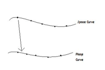
Figure 2. Projection problem for curves vs. projection problems for finite ordered sets of points

8. Directions of further research

The projection criteria developed in Section 4 reduce the problem of object-image correspondence for curves under a projection from $\mathbb{R}^{3}$ to $\mathbb{R}^{2}$, to a variation of the group-equivalence problem for curves in $\mathbb{R}^{2}$. We use differential signature construction [calabi98] to address the group-equivalence problem. In practical applications, curves are often presented by samples of points. In this case, invariant numerical approximations of differential invariants presented in [calabi98, boutin00] may be used to obtain signatures. Differential invariants and their approximations are highly sensitive to image perturbations and, therefore, are not practical in many situations. Other types of invariants, such as semi-differential (or joint) invariants [vang92-1, olver01], integral invariants [sato97, hann02, feng09] and moment invariants [hu62] are less sensitive to image perturbations and may be employed to solve the group-equivalence problem. One of our future projects is to develop variations of Algorithms 30 and 32 that are based on alternative solutions of the group-equivalence problem.

One of the essential contributions of [stiller06, stiller07] is the definition of an object/image distance between ordered sets of $m$ points in $\mathbb{R}^{3}$ and $\mathbb{R}^{2}$, such that the distance is zero if and only if these sets are related by a projection. Since, in practice, we are given only an approximate position of points, a “good” object/image distance provides a tool for deciding whether a given set of points in $\mathbb{R}^{2}$ is a good approximation of a projection of a given set of points in $\mathbb{R}^{3}$. Defining such object/image distance in the case of curves is an important direction of further research.

Although the projection algorithm presented here may not be immediatly applicable to real-life images, we consider this work to be a first step toward the development of more efficient algorithms to determine projection correspondence for curves and other continuous objects – the problem whose algorithmic solution, for classes of projections with large degrees of freedom, does not seem to appear in the literature.

Acknowledgements: This project was inspired by a discussion with Peter Stiller of paper [stiller07] during IS&T/ SPIE 2007 symposium. We also thank Hoon Hong and Peter Olver for discussions of this project.