Estimating Self-Sustainability in Peer-to-Peer Swarming Systems

Abstract

Peer-to-peer swarming is one of the de facto solutions for distributed content dissemination in today’s Internet. By leveraging resources provided by clients, swarming systems reduce the load on and costs to publishers. However, there is a limit to how much cost savings can be gained from swarming; for example, for unpopular content peers will always depend on the publisher in order to complete their downloads. In this paper, we investigate such a dependence of peers on a publisher. For this purpose, we propose a new metric, namely swarm self-sustainability. A swarm is referred to as self-sustaining if all its blocks are collectively held by peers; the self-sustainability of a swarm is the fraction of time in which the swarm is self-sustaining. We pose the following question: how does the self-sustainability of a swarm vary as a function of content popularity, the service capacity of the users, and the size of the file? We present a model to answer the posed question. We then propose efficient solution methods to compute self-sustainability. The accuracy of our estimates is validated against simulations. Finally, we also provide closed-form expressions for the fraction of time that a given number of blocks is collectively held by peers.

1 Introduction

Peer-to-peer swarming, such as used by BitTorrent [1], is a scalable and efficient way to publish content in today’s Internet. Peer-to-peer swarming has been widely studied during the last decade, and its use by enterprises is steadily growing [2, 3, 4, 5]. By leveraging resources provided by clients, peer-to-peer swarming decreases costs to publishers, and provides scalability and system robustness. As demand for content increases, system capacity scales accordingly, as all clients collaborate with each other while downloading the desired content. As the demand for multimedia files and the size of these files increase, peer-to-peer swarming systems have become an important content dissemination solution for many content providers [4, 5].

However, there is a limit on how much savings can be gained from swarming techniques. For example, in the case of unpopular content, peers must rely on the publisher in order to complete their downloads. In this paper, we investigate such a dependence of peers on a publisher.

A swarm is a set of peers interested in the same content (file or bundle of files [6]) that exchange blocks of the files among themselves. We consider a scenario where each swarm includes one stable publisher that is always online and ready to serve content. The corresponding system is henceforth referred to as a hybrid peer-to-peer system, since peers can always rely on the publisher if they cannot find blocks of the files among themselves. If all blocks are available among the peers, the swarm is referred to as self-sustaining. Quantifying swarm self-sustainability, defined as the fraction of time during which the swarm is self-sustaining, is useful for provisioning purposes. The larger the swarm’s self-sustainability, the lower the dependency of peers on the publisher, and the lower the bandwidth needed by the publisher to serve the peers.

The primary contribution of this paper is a model to study swarm self-sustainability. We use a two-layer model to quantify swarm self-sustainability as a function of the number of blocks in the file, the mean upload capacity of peers and the popularity of a file. The upper layer of our model captures how user dynamics evolve over time, while the lower layer captures the probability of a given number of blocks being available among the peers conditioned on a fixed upper layer population state. Our model is flexible enough to account for large or small numbers of blocks in the file, heterogeneous download times for different blocks, and peers residing in the system after completing their downloads. We derive closed-form expressions for the distribution of the number of blocks available among the peers and apply them to show that self-sustainability increases as a function of the number of blocks in the file. The derived expressions involve sums and subtractions of large numbers, and are amenable to numerical errors. Hence, we present an efficient algorithm to compute the swarm self-sustainability that avoids these problems. We then numerically investigate the minimum popularity needed to attain a given self-sustainability level. Finally, we validate the estimates made by the model against detailed simulations.

The remainder of this paper is organized as follows. After providing a brief background into swarming systems in §2, in §3 we propose our model. In §LABEL:sec:instant we present an efficient algorithm to solve the proposed model followed by analytical results in §LABEL:sec:analytical. In §4 we evaluate our model against experiments. In §5 we discuss some limitations and caveats of our model, §6 presents the related work and §7 concludes the paper.

2 Swarming Systems Primer

A swarm is a set of peers concurrently sharing content of common interest. Content might be a file or a bundle of files that are distributed together. The content is divided into blocks that peers upload to and download from each other. Since there is no interaction between peers across swarms, each swarm can be studied separately.

BitTorrent is one of the most popular applications that uses peer-to-peer swarming for content dissemination, and we will use it to illustrate how swarming works. Unlike a traditional server-based system, BitTorrent includes a tracker that promotes the interaction of participating peers. The identities of the trackers are announced to peers in torrent files, which can be found and downloaded through search engines such as Torrent Finder [7]. Peers periodically query the tracker to obtain a random subset of other peers in the swarm in order to exchange (upload and download) blocks with them. Peers also discover new neighbors from other peers, in addition to the tracker, when the Peer Exchange (PEX) extension is enabled.

There are two kinds of peers in the system: seeds and leechers. Seeds are peers that have completed their downloads and only upload blocks. Leechers are peers that have not completed their downloads and are actively downloading (and uploading) blocks of the file. Thus, leechers turn into seeds upon completing their downloads. Leechers adopt a tit-for-tat incentive strategy while downloading the file, i.e., leechers preferentially upload content to other leechers that reciprocate likewise, and “choke” or ignore leechers that do not reciprocate.

As many leechers may leave the system immediately after completing the download, content publishers often support a stable seed that we refer to as the publisher. A publisher is guaranteed to have all of the blocks constituting the file. In the rest of this paper we assume that each swarm includes one publisher.

BitTorrent peers adopt the rarest first policy to decide which blocks to download from their neighbors. According to the rarest first policy, a peer prioritizes the rarest blocks when selecting the ones to download next. We say that a peer is interested in another peer if the latter can provide blocks to the former. Since rarest first guarantees a high diversity of blocks in the system, any peer is almost always interested in any other peer, which in general yields high system performance [8].

Note, however, that in BitTorrent peers only have local information about the system. Hence, they can only implement a local rarest first policy. The intrinsic limit on the number of connections that a user can establish naturally provides each of them with only a myopic view of the system. Firewalls, NATs and other exogenous factors may also prevent users from establishing connections among themselves.

3 Model

In this section, we present our model to estimate swarm self-sustainability. Our model is hierarchical. The upper layer characterizes user dynamics, and the lower layer comprises a performance model used to quantify the distribution of blocks available among the peers, for a given state of the upper layer model. We present each of the layers, in §3.1 and §3.2, respectively, and then introduce the metric of interest in §3.3.

3.1 User Dynamics Model

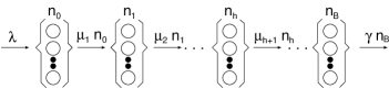
Figure 1: User dynamics. In stage $h$, there are ${n}_{h}$ users, each user owning $h$ blocks, $0\leq h\leq{B}$.

A file consists of ${B}$ blocks. Requests for a file arrive according to a Poisson process with rate $\lambda$. We further assume that the time required for a user to download its $j^{th}$ block is a random variable with mean $1/\mu_{j}$, $1\leq j\leq B$. After completing their downloads, peers remain in the system for a time with mean $1/\gamma$.

We model user dynamics with $({B}+1)$ M/G/$\infty$ queues in series. Each of the first $B$ M/G/$\infty$ queues models the download of a block, and capture the self-scaling property of BitTorrent swarms, i.e., each peer brings one unit of service capacity to the system. The last queue captures the residence time of seeds (see Figure 1).

The system state is characterized by a $({B}+1)$-tuple, ${\bf n}=({n}_{0},{n}_{1},{n}_{2},\ldots,{n}_{{B}})$, where ${n}_{h}$ represents the number of customers in queue $h$, i.e., the number of users that have downloaded $h$ blocks of the file, $0\leq h\leq{B}$. We denote by ${\bf N}$ the random variable characterizing the current state of the upper layer model and by ${\bf n}$ its realization. The number of peers in the system is referred to as $n$, $n=\sum_{i=0}^{B}n_{i}$.

Peers arrive according to a Poisson process with rate $\lambda$ to queue 0 and transit from queue $h$, also referred to as stage $h$, to queue $h+1$ ($0\leq h\leq{B}-1$) with rate $\mu_{h+1}$, the download rate of the $(h+1)^{th}$ block downloaded by a peer. The mean residence time in queue ${B}$ captures the mean time that peers remain in the system after completing their downloads, $1/\gamma$. Setting $\gamma=\infty$ models the case where all peers immediately leave the system after completing the download. Throughout this paper, unless otherwise stated, we assume that the mean download times of all blocks are the same, $1/\mu_{j}=1/\mu$, $1\leq j\leq B$. Nevertheless, all results are easily extended to the case where the mean time it takes for a user to download its $j^{th}$ block is $1/\mu_{j}$.

Let $\pi({n}_{0},\ldots,n_{{B}})$ be the joint steady state population probability distribution, $\pi(n_{0},\ldots,n_{B})=P({\bf N}=(n_{0},\ldots,n_{B}))$, of finding ${n}_{h}$ users in the $h^{th}$ queue, $0\leq h\leq{B}$, and let $\pi_{h}({n}_{h})=P(N_{h}=n_{h})$, $h=0,\ldots,B$, be the corresponding marginal probability. The steady state distribution of the queueing system has the following product form,

$$\pi({n}_{0},\ldots,{n}_{{B}-1},{n}_{{B}})=\prod_{h=0}^{{B}}\pi_{h}({n}_{h})=\frac{(\lambda/\gamma)^{{n}_{B}}}{{n}_{B}!}e^{-\lambda/\gamma}\prod_{h=0}^{{B}-1}\left(\frac{\rho^{{n}_{h}}}{{n}_{h}!}e^{-\rho}\right)$$ (1)

where $\rho=\lambda/\mu$ is the load of the system (refer to Table 1 for notation).

3.2 Performance Model For a Given Population State

parameters
$\lambda$	mean arrival rate of peers (peers/s)
$1/\mu$	mean time to download a block (s)
$\rho=\lambda/\mu$	mean load of the system (per stage)
${B}$	number of blocks in file
$1/\gamma$	mean residence time of seeds
variables
${n}_{h}$	number of users that own $h$ blocks
${{\bf n}}{=}{({n}_{0}}{,}{\ldots},{{n}_{{B}})}$	upper layer state
$\pi({\bf n})$	steady state probability of state ${\bf n}$
$n=\sum_{i=0}^{{B}}{n}_{i}$	number of peers in the system
${V}$	number of blocks available among the peers
metrics
$p({v})=P({V}={v})$	probability of ${v}$ blocks being available among peers
${A}{=}p({B})$	swarm self-sustainability

Table 1: Table of notation. Vectors are denoted by bold face symbols. Unless otherwise stated, $\gamma=\infty$ in which case $n_{B}=0$. When referring to block availability, it is subsumed availability among peers (excluding publisher).

We now describe the lower layer of the model. Given the current population state, ${\bf n}=({n}_{0},\ldots,{n}_{{B}})$, our goal is to determine the distribution of the number of blocks available among the peers. We begin by stating our key modeling assumption.

Uniform and independent block allocation: In steady state, the set of blocks owned by a randomly selected user in stage $h$ is chosen uniformly at random among the ${B\choose h}$ possibilities and independently among users.

A user $u$ in stage $h$, $0\leq h\leq{B}$, has a signature $s_{h,u}\in\{0,1\}^{B}$, defined as a ${B}$ bit vector where the $i^{{th}}$ bit is set to 1 if the user has block $i$ and 0 otherwise. Each user in stage $h$ owns $h$ blocks and has one of ${{B}\choose h}$ possible signatures.

Under the uniform and independent block allocation, signatures are chosen uniformly at random and independently among users; the latter is clearly a strong assumption since in any peer-to-peer swarming system the signatures of users are correlated. Nevertheless, in §4 we show that the effect of such correlations on our metric of interest, swarm self-sustainability, is negligible in many interesting scenarios. Therefore, we proceed with our analysis under such an assumption.

Let $S_{h,u}$ be the random variable denoting the signature of the $u^{th}$ user in stage $h$, and $s_{h,u}$ its realization, $1\leq u\leq n$. The sample space of the lower layer model, $\Omega_{{\bf n}}$, for a given state of the upper layer, ${\bf n}$, is the set of all $\{0,1\}^{Bn}$ bit vectors in which element $B(u-1)+i$ equals one if the $u^{th}$ user has block $i$, and zero otherwise, $1\leq u\leq n$, $1\leq i\leq B$. An element in $\Omega_{{\bf n}}$ is the concatenation of $n$ bit vectors of size $B$ each. $\Omega_{{\bf n}}$ has cardinality $|\Omega_{{\bf n}}|=\prod_{h=0}^{{B}}{{{B}\choose h}}^{{n}_{h}}$. Then, under the uniform and independent block allocation assumption,

$$P(S_{1,1}{=}s_{1,1}{,}\ldots{,}S_{B,{n}_{B}}{=}s_{B,{n}_{B}}|{\bf N}={\bf n}){=}\frac{1}{|\Omega_{{\bf n}}|}$$ (2)

In the next section, we relate the upper and lower layer models, showing how  (1) and  (2) yield the key metric of interest, namely, swarm self-sustainability.

3.3 Self-Sustainability

We now define the key metric of interest, swarm self-sustainability. Let $V$ denote the steady state number of blocks available among the peers. Denote by ${p}({v})$ the steady state probability that ${v}$ blocks are available among the peers,

$$p({v})=P(V={v})=\sum_{{\bf n}\in\mathbb{N}^{B+1}}P(V={v}|{\bf N}={{\bf n}})\pi({\bf n})$$ (3)

Definition 3.1

The swarm self-sustainability, ${A}$, is the steady-state probability that the peers have the entire file,

$$A=p(B)$$ (4)

Definition 3.1 together with equation (3) yield,

$${A}=\sum_{{\bf n}\in\mathbb{N}^{B+1}}P(V={B}|{\bf N}={{\bf n}})\pi({\bf n}){=}\sum_{{\bf n}\in\mathbb{N}^{B+1}}P(V={B}|{\bf N}={{\bf n}})\frac{(\lambda/\gamma)^{{n}_{B}}}{{n}_{B}!}e^{-\lambda/\gamma}\prod_{h=0}^{{B}-1}\left(\frac{\rho^{{n}_{h}}}{{n}_{h}!}e^{-\rho}\right)$$ (5)

The second equality in  (5) follows from (1). $P(V={B}|{\bf N}={\bf n})$ is obtained from (2) (see Appendix A).

We denote the swarm self-sustainability for a given value of $B$ and $\rho$ as $\hat{{p}}({B},\rho)$. The Bonferroni inequalities [10], which generalize the inclusion/exclusion principle, applied to (LABEL:d0), yield upper and lower bounds on $\hat{{p}}({B},\rho)$,

$$1-Be^{-(B+1)\rho/2}\leq\hat{{p}}({B},\rho)\leq 1-Be^{-(B+1)\rho/2}+{(B(B-1)/2)}e^{-2(B+1)\rho/3}$$ (6)

It is easy to show that if $\rho\geq 1.6$ and $B\geq 4$ then $1-Be^{-(B+1)\rho/2}+{(B(B-1)/2)}e^{-(B+1)\rho 2/3}\leq$ $\qquad 1-(B+1)e^{-(B+2)\rho/2}$, from which the result follows by comparing $\hat{{p}}({B},\rho)$ and $\hat{{p}}({B}+1,\rho)$. $\Box$

The key insight of Theorem LABEL:theo:filesize can be easily explained in terms of the busy periods of the proposed model. The busy period is defined as an uninterrupted interval during which the swarm is self-sustaining. As the file size increases, the number of blocks that need to be maintained increases linearly but the busy period of the system increases exponentially [6]. Indeed, as the file size increases the availability gain compensates the overhead to maintain a larger number of blocks, and the self-sustainability increases.

4 Evaluation

In this section we report $(a)$ a validation of the proposed model, against detailed simulations, showing that despite the simplifying assumptions considered in our model, it captures how self-sustainability depends on different system parameters and $(b)$ results on the minimum popularity to attain a given self-sustainability level.

4.1 Experimental Setup

Our simulation experiments were conducted using the Tangram-II modeling environment [11]. Tangram-II is an event-driven, object oriented modeling tool. The three main objects in our simulations are the tracker, the peer and the seed. Their implementations are based on the official BitTorrent protocol description [1, 8]. Every time a peer enters the system, receives a block or leaves, we record the event in our logs, the current timestamp, peer id, and signature (see  §1). 

4.1.1 Simulator and Protocol Descriptions

When a peer $P$ joins the system, it receives a random list of fifty other peers from the tracker, which constitutes its peer set. Throughout the simulation, as peers leave the system the size of the peer set of $P$ may dwindle to less than twenty. Once the peer set size is less than twenty, $P$ requests additional neighbors from the tracker. The set of peers to whom $P$ offers content blocks is a subset of its peer set, referred to as the active peer set.

BitTorrent proceeds in rounds of ten seconds. By the end of each round, peer $P$ runs the tit-for-tat incentive mechanism. According to this mechanism, $P$ reciprocates contents with those neighbors that contributed in the previous round. $P$ selects $r$ of those peers that contributed in the last round to add to its active peer set ($r\leq 4$). In the next round, the active peer set of $P$ will consist of the $r$ aforementioned peers plus $5-r$ additional peers selected uniformly at random out of its peer set. This random selection of peers is referred to as optimistic unchoke, performed to allow peers to get bootstrapped as well as to let them learn about new neighbors. Finally, peers select blocks to download using the rarest first algorithm, except for the first four blocks, which are chosen uniformly. Each block of the file is divided into sixteen sub-blocks. After selecting the blocks to download, peers can get different sub-blocks (of the same block) from different neighbors concurrently. A block can be uploaded after all its sub-blocks are downloaded, assembled and checked using the block hash key.

In our experiments we observe that self-sustainability decreases with the size of the active peer sets. That is because, if the active peer sets are large, each peer splits its bandwidth across many other peers and blocks take longer to get replicated in the network. As mentioned above, we select an active peer set of size five, which is adopted by many BitTorrent implementations.

In our experiments the seed behaves as a standard peer, except that it $(i)$ initially owns all blocks and $(ii)$ is altruistic, hence does not execute the tit-for-tat algorithm. We did not implement the mechanism used by peers to download their last block, also known as end game mode [1]. This is inconsequential, though, since the end game mode does not significantly affect the steady state behavior of the system (see §4.2.1 and [12]).

4.1.2 Experimental Parameters

The configuration of our experiments consists of torrents that publish a file of size $S$ divided into $B$ blocks of size $s$, $s=256$KB, a typical block size in BitTorrent. The number of blocks in the file, $B$, takes values 16, 50, 100 and 200, which corresponds to files of size 4MB, 12MB, 25MB and 51MB, respectively. Note that if a swarm is constituted of multiple files which can be downloaded separately, we are interested in analyzing the self-sustainability of each individual file. A file of size 51MB already yields self-sustainability larger than 0.9 for $\lambda>0.05$ peers/min (see Figure 3). Simulations to analyze such a steep increase in self-sustainability (see Figure 3) quickly requires prohibitively large execution times and significant variability in the metrics of interest across runs. For this reason, we focused on quantitatively validating our model for files with up to 200 blocks, but also use the model to analyze files of size greater than 200 blocks.

The uplink capacity of each peer is $39$KBps, which corresponds to $\mu=39/256=0.15$ blocks/s, a typical effective capacity for BitTorrent peers [13, Figure 1]. The publisher maximum upload capacity is the same as that of a peer. A publisher that contributes the same capacity as an ordinary peer might correspond to either a domestic user or a commercial publisher that supports a large catalog of titles and only provides enough capacity for each swarm so as to allow peers to complete their downloads at rate $\mu$. The peer arrival rate is varied according to the experimental goals between $(.25,.5,1,2,\ldots,9)$ peers/min, as described next.

4.2 Model Validation

Our analytical model makes a number of simplifying assumptions as described in §3. In what follows, our goal is to show that even with those simplifying assumptions, discussed in §4.2.1, our model still captures swarm self-sustainability in a realistic setting, as shown in §4.2.2.

4.2.1 Validating Model Assumptions

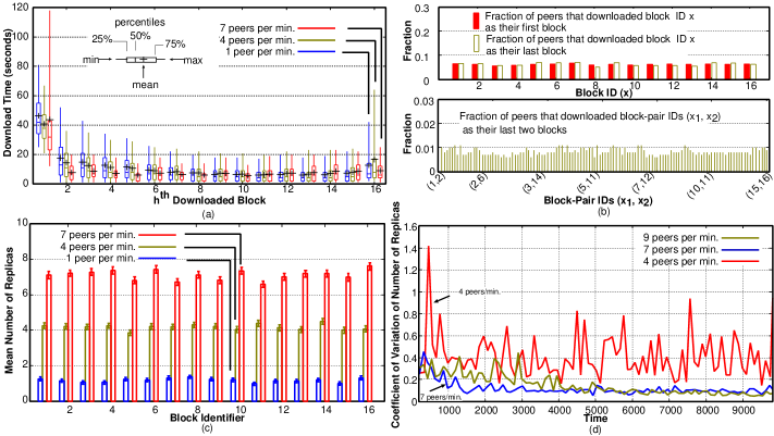
Figure 2: $(a)$ Download times of $h^{th}$ block downloaded by a peer. The boxplots show the four quartiles and crosses indicate means. $(b)$ Top: shaded (resp., light) rectangles are fractions of peers that download block $x$ as their first (resp., last) block. Bottom: fraction of peers that download block-pair $(x_{1},x_{2})$ as their last two blocks. $(c)$ Mean number of replicas of each block with 95% confidence intervals. $(d)$ Coefficient of variation of number of replicas of blocks versus time.

Our aim in this section is to validate $(a)$ that the mean download times of blocks are roughly the same (an exception being the first block downloaded by the peers), i.e., $\mu_{h}=\mu$, $2\leq h\leq B$ (see  §3.1) and $(b)$ that the signatures of the users are uniformly distributed (see §1).

Figure 2(a) shows the download time of the $h^{th}$ block downloaded by a peer. The boxplots and lines show the distribution quartiles and minimum and maximum values. Crosses indicate means download times of blocks, which are approximately the same, except for the first and last blocks. In particular, even though our simulator ignores the end game mode [12], in general peers do not experience difficulty finding a neighbor from whom to download their last block. The median of the last block is roughly the same as the one observed for the other blocks, and the mean is only slightly larger. The first block requested by a peer, however, takes longer to be downloaded. This happens because a peer can only download its first block after being optimistically unchoked (see  §4.1.1). Although this affects the time spent by peers in stage zero of our model and as a consequence the total download time, it is inconsequential to our self-sustainability estimates (the time that peers remain in stage zero of the upper layer model has no influence in our results). While BitTorrent peers download their first block, they cannot contribute to self-sustainability as they have no content to provide (see  §4.1.1).

Our second goal is to study the users’ signatures distribution (§1). For this purpose, we validated that the first two and last two blocks downloaded by a user are indeed uniform and then studied one of the consequences of the uniform and independence assumption, namely, that the number of replicas of each block in the system is well balanced.

Figure 2(b) (top) shows, for each block, the fraction of peers that downloaded that block as their first block (shaded bars). The figure was generated from independent samples: every 500 seconds, one user owning one block was randomly selected, and the identity of its block was recorded (the same procedure was repeated for users owning all but one block of the file (light bars)). Similarly, Figure 2(b) (bottom) shows, for every $B(B-1)$ block-pair, the fraction of peers that downloaded that pair as their first two blocks. Figure 2(b) indicates that the first and last blocks downloaded by users, as well as the first downloaded block-pair, are approximately uniformly distributed (the same procedure was repeated for users owning all but two blocks, with similar results).

Figure 2(c) shows the mean number of replicas of each block (including the one stored at the publisher) for $\lambda=1$ peer/min, $4$ peers/min and $7$ peers/min. The mean number of replicas of each block is around $\rho({B}-1)/2+1$, which corresponds to a well balanced system (see §LABEL:sec:minloadanl). Figure 2(d) corroborates this claim by showing the coefficient of variation of the number of replicas of blocks as a function of time. Let $r_{i,t}$ be the number of replicas of block $i$ at time $t$. The mean number of replicas of blocks at time $t$ is $\mu_{t}=\sum_{i=1}^{B}r_{i,t}/B$ and the coefficient of variation is $c_{t}=\sqrt{(\sum_{i=1}^{B}(r_{i,t}-\mu_{t})^{2}/B)}/\mu_{t}$. Figure 2(d) indicates that throughout the simulation, the coefficient of variation is usually smaller than 0.8, which means that the number of replicas of blocks has a low variance. In a system where users signatures are uniform and independent we would observe similar behavior.

4.2.2 Validating Model Estimate of Self-Sustainability

To study how content popularity impacts self-sustainability, we simulated BitTorrent in the setting described in §4.1.2, varying the arrival rate of peers, $\lambda$, from 1 peer/minute to 8 peers/minute, in increments of 1 peer/minute, while maintaining all other parameters fixed. Equivalently, this corresponds to an increase in the load, $\rho=\lambda s/{\mu}$, from 0.1 to 0.8. Each simulation lasted for 10,000s. Twenty one independent simulations were executed for each value of $\lambda$, and used to compute 95% confidence intervals. The same experiment is repeated for $B=16$, $50$, $100$ and $200$.

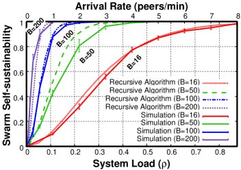
Figure 3: Model validation. Swarm self sustainability as a function of the system load. Results obtained with recursive algorithm and simulations (with 95% confidence intervals) are plotted with dotted and solid lines, respectively.

Figure 3 shows self-sustainability, $A$, as a function of the content popularity, $\lambda$, for $B=16,50,100$ and $200$. For unpopular contents, $\lambda=1$ peer/min, and small files, $B=16$, swarm self-sustainability is around 0.1 and the publisher needs to frequently provide blocks that are unavailable among the peers. As the popularity of the files increases, swarm self-sustainability increases and content is available even in the absence of the publisher. For $\lambda=8$ peers/min, the fraction of time at which the publisher needs to provide blocks to peers is close to zero.

Figure 3 indicates that the results obtained with our model are close to those obtained through simulation. Even assuming that the mean download times of all blocks are the same ($\mu_{h}=\mu$, for $1\leq h\leq B$), the model was able to capture the self-sustainability observed in our simulations. We also repeated the simulations with heterogeneous peer upload capacities, for $B=16$ (the upload rate distribution taken from the measured data used to generate Figure 1 in the BitTyrant study [13]) and our results did not qualitatively change (details in [9]).

Consider now the impact of file size on swarm self-sustainability. Figure 3 shows that for a fixed content popularity, as file size increases, self-sustainability increases. This is in accordance with Theorem LABEL:theo:filesize, and reflects the fact that, as file size increases, peers stay longer in the system and the coverage, defined as the mean number of users in the system, increases. The higher the coverage, the greater the self-sustainability of the swarm. In fact, as file size increases, the number of blocks that needs to be maintained by the publisher increases linearly but the availability gain increases exponentially [6].

4.3 Popularity to Attain High Self-Sustainability

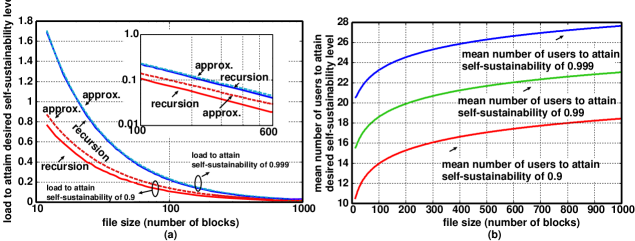
Figure 4: Larger files yield increased availability. $(a)$ $x$-axis, file size. $y$-axis, necessary load ($\rho^{\star}=\lambda/\mu$) to attain self-sustainability greater than 0.9 (red) and 0.999 (blue). The results obtained using the approximation (LABEL:eq:rhostar) are also shown. $(b)$ the mean number of users in the system, $B\rho^{\star}$, to attain a desired self-sustainability level.

We now address the following question: what is the minimum file popularity (or load) needed to attain a given self-sustainability? Answering this question is useful not only for publisher dimensioning but also for other strategic decisions such as how to distribute and bundle files across multiple swarms [6].

Recall that the load is defined as $\rho=\lambda/\mu$. Figure 4 shows the minimum load, $\rho^{\star}$, necessary to achieve high self-sustainability, $A^{\star}$ ($A^{\star}=0.9,0.999$), for file sizes varying between 2MB and 256MB ($B=8,\ldots,1,000$). This figure illustrates self-sustainability as predicted by the recursions contained in Theorem LABEL:theo:efficientalgo, eq. (LABEL:dimsimple) and the approximation (LABEL:eq:rhostar). Figure 4(a) suggests that when the goal is to find the minimum popularity to attain a high self-sustainability level, equation (LABEL:eq:rhostar) can be used to approximate $\rho^{\star}$. However, if the goal is to compute self-sustainability under different loads and for different files sizes, as illustrated by Figure 3, the recursion provided by Theorem LABEL:theo:efficientalgo needs to be used.

Figure 4(a) indicates that the popularity, $\rho^{\star}$, needed to attain a high degree of self-sustainability increases as the file size, $B$, decreases. In particular, the zoom in the figure shows that $\log\rho^{\star}$ is linear in $\log B$. The comments made at the end of  §4.2 to explain Figure 3 also apply here. Peers take longer to download larger files, which increases block availability. Nevertheless, the benefits of leveraging peer-to-peer swarming can be noted even for small files. Figure 4(a) shows that for a file of $4$MB ($B=16$), an arrival rate of $8$ peers/min (which corresponds to a load of 0.8) already yields a very high self-sustainability.

More insights on how file size impacts self-sustainability are obtained from Figure 4(b). Figure 4(b) plots the mean number of users in the system, also referred to as the mean coverage [6], necessary to attain a high level of self-sustainability. The curves in Figure 4(b) correspond to the the respective ones in Figure 4(a) multiplied by $B$. The main insight shown in this example is that the coverage necessary to attain a given self-sustainability level slowly increases as a function of $B$. As the file size increases, a slightly larger population suffices to attain a given self-sustainability level. For instance, for a file of size 10 a coverage of 20 is necessary to attain self-sustainability of 0.999, whereas a coverage of 29 suffices to achieve the same self-sustainability if the file has 1,000 blocks.

5 Discussion

Next, we discuss the assumptions adopted to yield a tractable model.

Uniformity and independence assumptions: In the performance model presented in §3.2 we assume that the signatures of users are drawn uniformly and independently at random. In particular, we do not account for correlations among users’ signatures. Although such correlations are present in practice, our simulations have indicated that the independence assumption is appropriate in order to capture the self-sustainability of swarms.

In the user dynamic model presented in §3.1 we make the following assumptions: $(i)$ peers arrive according to a Poisson process with rate $\lambda$ (steady state assumption), $(ii)$ the download times of all blocks have the same mean, $1/\mu$ (smooth download assumption) and $(iii)$ users leave the system immediately after completing their downloads, $\gamma=\infty$ (self-regarding users assumption). We discuss each of these in turn.

Steady state assumption: It has been shown in  [6, Section 4.3.4] that a vast number of long-lived swarms have relatively stable mean arrival rates over periods of months. Our model can be used to predict the self-sustainability of such swarms.

Smooth download assumption: Under this assumption, the capacity of the system scales perfectly with the number of users. Our simulations indicate that the mean download time of the first and last blocks are slightly larger than the others. Although our model has the flexibility to capture such asymmetries (see observation two in §LABEL:sec:bwratio), we show that their implications in the estimates of self-sustainability are not significant (see §4.2.1).

Self-regarding users assumption: Our model has the flexibility to account for users that stay in the network after completing their downloads. However, in today’s BitTorrent users have no incentive to stay in the system after obtaining the files of their interest. Therefore, we focus on the worst case scenario in which users, not having incentives to linger in the system after completing their downloads, depart immediately.

Finally, in our simulations we consider a publisher that is always online and that behaves like a typical peer.

Typical peer-like publisher: Our simulations indicate that if the publisher has the same capacity as a typical peer, the smooth download assumption holds and the swarm self-sustainability estimates of our model are accurate. Coping with intermittent publishers and devising dynamic bandwidth allocation strategies according to which the smooth download assumption holds is non trivial [14], and is subject of future work.

6 Related Work and Discussion

Modeling of Peer-to-Peer Swarming Systems

The literature on availability [15], performance [16] and incentive issues [13] in BitTorrent-like swarming systems is vast. Nevertheless, to our knowledge this paper presents the first analytical model for publisher dependency estimation. We are unaware of related analytical work that analyzed swarm self-sustainability taking into account the fact that files are divided into multiple blocks, a very fundamental characteristic of these systems.

For large populations, Massoulié and Vojnovic [17] used a coupon collector model to show that asymptotically the distribution of blocks across the population is well balanced, and does not critically depend on the block selection algorithm used by the peers. Qiu and Srikant [16] and Fan et al. [18] also considered the large population regime, and used fluid approximations and differential equations to model the system assuming that the efficiency is always high. In this paper we are particularly interested in the small population regime. For small populations, Markov Chain (MC) models have been proposed by Yang and Veciana [19], providing insights on the performance of the system but not dealing with the problem of block availability among peers. Norros and Reittu [20], using a different model, studied the dissemination of a two-block file in a closed network accounting for the availability of the blocks. In this paper, we consider an open network and propose a model which can be used to estimate self-sustainability of files of arbitrary size.

In this work we studied the implications of the content popularity on the self-sustainability of swarms. In a real time setting, Leskela et al. [21] pointed out a phase transition in the stability of the peer-to-peer system as a function of the content popularity. In contrast, our system is always stable. Norros et al. [22] imply a phase transition of the mean broadcast times as a function of the departure rate of seeds. In this paper we are concerned with self-sustainability.

Hybrid Peer-to-Peer Swarming Systems

The literature on the use of peer-to-peer swarming systems for enterprise content delivery is rapidly growing  [23, 24, 25]. The methodology usually consists of defining an optimization problem to be solved by the publishers and then showing how different system parameters affect the optimal bandwidth allocation strategy. The approach we take in this paper is different. We are interested in the minimum fraction of time that the publisher must be active so as to guarantee that all blocks are always available.

Ioannidis and Marbach [26] study how quickly the bandwidth available at the server has to grow as the number of users increases. For this purpose they consider two query propagation mechanisms, the random walk and the expanding ring. Here, on the other hand, we assume that peers can always find the blocks they need in case they are available. While  [26] focuses on the control plane and it’s asymptotic analysis, here we focus on the data plane and account also for small files.

Menasche et al. [6], Wong et al. [27] and Susitaival et al.  [28] propose models for content availability in BitTorrent without accounting for the fact that files are divided into blocks. Our model differs from  [6, 27, 28] in that we $(a)$ consider a hybrid peer-to-peer system, in which a publisher is always available and $(b)$ account for the fact that the file is divided into blocks. Finally, explicit scheduling of blocks exchanges to minimize peer download times was studied by Mundinger et al. [29]. In this paper we assume that peers exchange blocks using only local information, as in BitTorrent.

Balls and Bins

The derivation of some of our results fit into the balls and bins framework. Each user is allocated a set of blocks (balls) each of which must correspond to a different identifier (bin). In the context of balls and bins, a set of balls each of which must be allocated in a different bin is referred to as complex [30]. Previous work on the allocation of complexes into bins appears in Mirakhmedov and Mirakhmedov [31], Kolchin et al. [30, Chapter VII], and references therein. In particular, the definition of $\psi_{h}(i,m)$ in this paper was inspired by [32, Figure 1].

In a peer-to-peer setting, balls and bins were used by Simatos et al. [33] to study the duration of the regime during which the system is saturated because capacity is smaller than demand. The scenario studied in this paper differs from  [33] in several aspects. For instance,  [33] considers a finite population of peers.

7 Conclusion

Peer-to-peer swarming systems are a powerful tool for content delivery, as reflected by the immense popularity of BitTorrent and the vast literature on the topic. However, most works in this area have focused on the dissemination of popular content, for which peer-to-peer systems are naturally suitable. In this work, we investigate the dependency of peers on a publisher that leverages peer-to-peer techniques for the dissemination of both popular and unpopular content. In particular, the latter deserve special attention, since unpopular content can represent a significant fraction of demand and revenue [34]. We believe that devising strategies for disseminating large catalogs of files leveraging peer-to-peer techniques is an important and interesting research area, and we see our model as a first attempt to shed light into the intrinsic advantages and limitations of peer-to-peer swarming systems for the dissemination of such catalogs.

Acknowledgements We are thankful to Carsten Schneider, author of Sigma [35], for his support using the package. This work was supported in part by the NSF under award numbers CNS-0519922 and CNS-0721779. Research of DSM also sponsored by a scholarship from CAPES/Fulbright (Brazil). Research of ESS, RML and AAAR is partially funded by research grants from CNPq and FAPERJ.

Appendix A An Expression of $P(V={B}|{\bf N}={\bf n})$

We now show how to obtain $P(V={B}|{\bf N}={\bf n})$ from (2). Recall that, given an upper layer state ${\bf n}$, $\Omega_{{\bf n}}$ is the lower layer sample space. Denote by ${\bf S}$ the random variable that represents the lower layer state, and by ${\bf s}$ its realization. Then

$$P(V={B}|{\bf N}={\bf n})=\sum_{{\bf s}:V={B},{\bf s}\in\Omega_{{\bf n}}}P({\bf S}={\bf s}|{\bf N}={\bf n})\stackrel{{\scriptstyle\eqref{uniformjoint}}}{{=}}\sum_{{\bf s}:V={B},{\bf s}\in\Omega_{{\bf n}}}1/|\Omega_{{\bf n}}|$$ (7)

Therefore, the problem of computing $P(V={B}|{\bf N}={\bf n})$ is reduced to that of counting the states in which all blocks are available among the peers. Using the inclusion/exclusion principle, $P({V}={B}|{\bf N}={\bf n})={|\Omega_{{\bf n}}|}^{-1}\sum_{i=0}^{{B}-1}(-1)^{i}{{B}\choose i}\prod_{j=1}^{{B}-1}{{{B}-i\choose j}}^{{n}_{j}}.$ In general, $P({V}={v}|{\bf N}={\bf n})$ is also obtained using the inclusion/exclusion principle [36, Section 4.2].

Appendix B Recursion to Compute $\psi_{h}(k,{v})$

Consider the scenario where $k$ blocks are available among the peers and an additional user contributes $h$ blocks. $\psi_{h}(k,{v})$ is the probability that ${v}$ blocks are available among the peers after accounting for the blocks contributed by the additional user. $\psi_{h}(k,{v})$ can be recursively computed,

$$\psi_{h}(k,{v})=\psi_{h-1}(k,{v}-1)\frac{B{-}{v}{-}h}{B{-}h{+}1}+\psi_{h-1}(k,{v})\frac{{v}}{B{-}h{+}1},\qquad 0\leq k,{v}\leq B,\quad 0<h\leq B$$ (8)

The base cases are $\psi_{0}(k,{v})=0$ if ${v}\neq k$ and $\psi_{0}(k,{v})=1$ if ${v}=k$. Note that the above recursion is convenient to avoid numerical problems since it only involves additions and multiplications of probabilities.

For presentation convenience, we consider an arbitrary ordering of the $h$ blocks contributed by the additional user. After contributing the first $h-1$ blocks, there are two cases to consider, $(i)$ ${v}$ blocks are available among the peers [and the $h^{th}$ block overlaps with a previously available block, an event which happens with probability ${v}/({B{-}h{+}1})$] or $(ii)$ ${v}-1$ blocks are available [and the $h^{th}$ block does not overlap with previously available blocks, an event which happens with probability $(B{-}{v}{-}h)/({B{-}h{+}1})$]. Cases $(i)$ and $(ii)$ correspond to the first and second terms in (8), respectively.

Appendix C Proof of Lemma LABEL:lemmaprob

We now show that (LABEL:mainrec) and (LABEL:umpvm) are equivalent. To this purpose, we consider an extended representation of the upper layer states. In such representation, the upper layer state, ${\bf n}^{\prime}$, is defined as follows.

Consider the users in the system ordered uniformly at random. The number of blocks owned by the $i^{th}$ user is denoted by ${n}^{\prime}_{i}$. The upper layer state is represented by vector ${\bf n}^{\prime}$. The dimension of ${\bf n}^{\prime}$ is $1\times n$, where $n$ is the number of users in the system.

Note that ${\bf n}$ is inferred from ${\bf n}^{\prime}$. Let $n_{l}({\bf n}^{\prime})$ be the number of users that have $l$ blocks when the state is ${\bf n}^{\prime}$. Since any permutation of the users in the system is equally likely, the steady state probability of state ${\bf n}^{\prime}$ is $\pi({\bf n}^{\prime})$,

$$\pi({\bf n}^{\prime})=\prod_{l=0}^{{B}-1}\left[\frac{\rho^{n_{l}({\bf n}^{\prime})}}{n_{l}({\bf n}^{\prime})!}e^{-\rho}\right]\frac{1}{n!}$$

The steady state probability of state ${\bf n}^{\prime}$, conditioned on the event that there are $n$ users in the system, is

$$\frac{\pi({\bf n}^{\prime})}{\sum_{\forall{\bf n}^{\prime}:|{\bf n}^{\prime}|=n}\pi({\bf n}^{\prime})}{=}\frac{\pi({\bf n}^{\prime})}{e^{-B\rho}(B\rho)^{n}/{n}!}=\frac{1}{B^{n}\prod_{l=0}^{{B}-1}{n_{l}({\bf n}^{\prime})!}}$$ (9)

The first equality follows from the fact that a superposition of $B$ Poisson processes with rate $\rho$ is a Poisson process with rate $B\rho$.

The key idea of the proof consists of partitioning the state space into sets $G_{h}(n)$, $0\leq h\leq{B}-1$, $0\leq n$. Set $G_{h}(n)$ contains states in which there are $n$ users in the system and ${n}^{\prime}_{n}=h$. $G_{h}(n)$ is defined as $G_{h}(n)=\{{\bf n}^{\prime}:{n}^{\prime}_{n}=h\textrm{ and }0\leq{n}^{\prime}_{j}\leq B-1,1\leq j<n\}$. The set containing all states in which there are $n$ users in the system, $G(n)$, is

$$G(n)=\cup_{h=0}^{B-1}G_{h}(n)=\{{\bf n}^{\prime}:0\leq{n}^{\prime}_{j}\leq B-1,1\leq j\leq n\}$$ (10)

Note that $G_{h}(n)$ is obtained from $G(n-1)$ by adding to each element of $G(n-1)$ a user that owns $h$ blocks,

$$G_{h}(n)=\{({\bf n}^{\prime},0)+h{\bf 1}_{n}:{\bf n}^{\prime}\in G(n-1)\}$$ (11)

${\bf 1}_{n}$ denotes a $1\times n$ vector in which all elements equal zero, except element $n$, which equals one. Let $p({v}|{{\bf n}^{\prime}})$ be the probability of ${v}$ blocks being available among the peers when the upper layer state is ${\bf n}^{\prime}$. If ${\bf n}^{\prime}\in G_{h}(n)$ ($n>0$),

$$p({v}|{{\bf n}^{\prime}})=\sum_{k=0}^{B}p(k|{{\bf n}^{\prime}-h{\bf 1}_{n}})\psi_{h}(k,{v}),\qquad{\bf n}^{\prime}\in G_{h}(n)$$ (12)

According to definition  (LABEL:umpvm),

$${p}_{n}({v}){=}\left[\sum_{{\bf n}^{\prime}\in G(n)}p({v}|{{\bf n}^{\prime}})\pi({\bf n}^{\prime})\right]\Big{/}\left[\sum_{{\bf n}^{\prime}\in G(n)}\pi({\bf n}^{\prime})\right]=\sum_{{\bf n}^{\prime}\in G(n)}p({v}|{{\bf n}^{\prime}})\frac{1}{B^{n}\prod_{l=0}^{{B}-1}{{n}_{l}({\bf n}^{\prime})!}}$$ (13)

where the first and second equalities follow from (10) and (9), respectively. Hence,

$$p_{n}({v})=\sum_{h=0}^{B-1}\sum_{{\bf n}^{\prime}\in G_{h}(n)}p({v}|{{\bf n}^{\prime}})\frac{1}{B^{n}\prod_{l=0}^{{B}-1}{{n}_{l}({\bf n}^{\prime})!}}{=}\sum_{h=0}^{B-1}\sum_{{\bf n}^{\prime}\in G_{h}(n)}\sum_{k=0}^{B}p(k|{{\bf n}^{\prime}-h{\bf 1}_{n}})\psi_{h}(k,{v})\frac{1}{B^{n}\prod_{l=0}^{{B}-1}{{n}_{l}({\bf n}^{\prime})!}}$$ (14)

$${=}\sum_{h=0}^{B-1}\sum_{k=0}^{B}\underbrace{\sum_{{\bf m}^{\prime}\in G(n-1)}p(k|{{\bf m}^{\prime}})\frac{1}{B^{n-1}\prod_{l=0}^{{B}}{{n}^{\prime}_{l}!}}}_{{p}_{n-1}(k)}\psi_{h}(k,{v})\frac{1}{B}{=}\sum_{h=0}^{B-1}\sum_{k=0}^{B}{p}_{n-1}(k)\psi_{h}(k,{v})\frac{1}{B}$$ (15)

where the first, second and third equalities follow from (10), (12) and (11), respectively. Note that the summands in  (15) for which $h>v$ or $k\in[0,v-h-1]\cup[v+1,B]$ are equal to zero, since in these cases $\psi_{h}(k,v)=0$. Therefore,  (15) yields (LABEL:mainrec).

Appendix D Probabilistic Derivation of  (LABEL:1okp1)

Next, we provide a probabilistic derivation of (LABEL:1okp1). An algebraic proof can be obtained using the Sigma package [35], applying a paradigm called creative telescoping [37].

Henceforth, we consider the case ${v}<{B}$ (the case ${v}={B}$ follows similarly). The probabilistic interpretation for (LABEL:1okp1) follows from the connection between $\psi_{h}(k,{v})$ and the hypergeometric distribution. Suppose we have an urn containing $B$ balls, $B-k$ of which are white (unavailable blocks) and $k$ are black (available blocks). $\psi_{h}(k,{v})$ is the probability of selecting without replacement $h$ balls, of which ${v}-k\leq h$ are white.

Consider now another experiment, namely selecting without replacement all balls from the urn. Let $J_{w}$ be the round in which the $w^{th}$ white ball is selected, $0<J_{1}<J_{2}<\ldots<J_{B-k}<{B}+1$. Let $W_{b}$ be the number of black balls selected between the $b^{th}$ and $b+1^{th}$ white, plus one. Equivalently, $W_{b}$ is the number of elements in the set $S=\{n\in\{0,\ldots,{B}\}:\textrm{ exactly $b$ white balls are selected before ball $n$}\}$. Then $W_{0}=J_{1}$, $W_{1}=J_{2}-J_{1}$, $\ldots$, $W_{k-1}=J_{k}-J_{k-1}$, and $W_{B-k}={B}+1-J_{i}$. Clearly, $\sum_{b=0}^{B-k}W_{b}={B}+1$. By symmetry, $E[W_{b}]=({B}+1)/(B-k+1)$ ($0\leq b\leq B-k$).

Now let ${v}-k$ be given, ${v}-k\in\{0,1,\ldots,{v}\}$. Let ${\bf 1}_{h}$ be the indicator equal to 1 if exactly ${v}-k$ white balls are selected among the first $h$ balls. Note that $E[{\bf 1}_{h}]=\psi_{h}(k,{v})$. Also, from the definition of $W_{{v}-k}$, we have $W_{{v}-k}=\sum_{h=0}^{{B}}{\bf 1}_{h}$. Therefore, $E[W_{{v}-k}]=\sum_{h=0}^{{B}}E[{\bf 1}_{h}]=\sum_{h=0}^{{B}}\psi_{h}(k,{v})=({B}+1)/(B-k+1)$.

Appendix E Proof of Theorem LABEL:theo:efficientalgo

Replacing (LABEL:1okp1) into  (LABEL:simplified1) yields,

$${p}_{n}({v}){=}\left\{\begin{array}[]{lll}1/B^{n},&n\geq 1,{v}=0&(i)\\ \sum_{k=0}^{{v}}p_{n-1}(k)(B+1)/(B(B-k+1)),&n\geq 1,0<{v}<B&(ii)\\ 1-\sum_{l=0}^{B-1}{p}_{n}(l),&n\geq 1,{v}=B&(iii)\\ 1,&n=0,{v}=0&(iv)\\ 0,&n=0,{v}\neq 0&(v)\end{array}\right.$$ (16)

In case $(ii)$, $p_{n}({v})=p_{n-1}({v})(B+1)/(B(B-{v}+1))+\sum_{k=0}^{{v}-1}p_{n-1}(k)(B+1)/(B(B-k+1))=p_{n-1}({v})(B+1)/(B(B-{v}+1))+p_{n}({v}-1)$ which yields (LABEL:dimsimple).

Appendix F Expression of $p_{n}({v})$ When $\gamma=\infty$

If $\gamma=\infty$, the closed-form expression for $p_{n}({v})$ is ${p}_{n}({v}){=}{B\choose{v}}\left(\frac{1+B}{B}\right)^{n}\sum_{l=0}^{{v}}{{v}\choose l}(-1)^{l}(B-{v}+l+1)^{-n}$, $n\geq 1,B>{v}\geq 0$, and ${p}_{n}(B)=1-\sum_{{v}=0}^{B-1}{p}_{n}({v})$.

Appendix G Self-Sustainability with Heterogeneous Download Times

We now present an efficient algorithm to compute swarm self-sustainability if the block download times, $\mu_{h}$, are not necessarily equal for all $h$, $1\leq h\leq B$.

Denote by $a_{h,r}({v})$ the probability that ${v}$ blocks are available among the peers conditioned on the presence of $r$ users in layer $h$ and all users being in layers $h$ up to $B$,

$$a_{h,r}({v})=P(V={v}\Big{|}{n}_{h}=r;{n}_{i}=0,i<h),\qquad 0\leq h\leq B,\qquad 0\leq r\leq M$$ (17)

$M$ is the maximum number of users per layer. The following recursion correctly computes $a_{h,r}$, $0\leq h\leq B$, $0\leq r\leq M$,

$$a_{h,r}({v}){=}\left\{\begin{array}[]{lll}{\displaystyle{\sum_{\begin{subarray}{c}i=0\end{subarray}}^{{v}}}}a_{h,r{-}1}(i)\psi_{h}(i,{v}),&{r\geq 1},h\neq B&(i)\\ \sum_{r=0}^{\infty}a_{h+1,r}({v})\pi_{h+1}(r),&r=0,h\neq B&(ii)\\ 1,&r=0,h=B,v=0&(iii)\\ 0,&r=0,h=B,v\neq 0&(iv)\\ \end{array}\right.$$ (18)

We approximate $A$ by its truncated version, $\overline{A}^{(M)}$, considering only states in which there are up to $M$ users in each layer of the system. Recall that $N$ is the maximum number of users in the system, $N=O(BM)$. A naive use of (18) yields an algorithm to compute $\overline{A}^{(M)}$ in time $O(B^{3}M)=O(B^{2}N)$.

In what follows, we show how to compute $\overline{A}^{(M)}$ in $O(NB\log B)$. For this purpose, we re-write the sum in  (18)$(i)$ as a convolution, which is computed in time $O(B\log B)$. Let

$$\widehat{a}_{h,r{-}1}(k)=a_{h,r{-}1}(k){k!}{(B{-}k)!},\quad 0\leq k\leq B\quad\textrm{ and }\quad\widehat{\psi}_{h}({v}-k)=1/({({v}{-}k)!}{(h{-}({v}{-}k))!}),\quad 0\leq k\leq{v}$$

Then, the following convolution correctly computes  (18)$(i)$, $\widehat{{{{a}}}}_{h,r}=\widehat{{{{a}}}}_{h,r-1}\otimes\widehat{{\psi}}_{h}$.

${a}_{h,r}$ is obtained from $\widehat{a}_{h,r}$ as

$$a_{h,r}({v})=\left\{\begin{array}[]{ll}({\widehat{a}_{h,r}({v})})/\left({({v}-h)!(B{-}{v})!{{{B}\choose h}}}\right),&0\leq{v}\leq B-1\\ 1-\sum_{i=0}^{{B}-1}a_{h,r}(i),&v=B\\ \end{array}\right.$$ (19)

Appendix H Derivation of  (LABEL:closedform)

We now show that (LABEL:closedform) follows from (LABEL:dimsimple2). The case ${v}=B$ follows trivially. For ${v}<B$, we show that (LABEL:closedform) satisfies (LABEL:dimsimple2), i.e., ${p}_{n}({v})-{p}_{n-1}({v})(1/(B-{v}+1))={p}_{n}({v}-1)$,

$${p}_{n}({v})-{p}_{n-1}({v})(1/(B-{v}+1))={B\choose{v}}\sum_{l=0}^{{v}}{{v}\choose l}(-1)^{l}(B-{v}+l+1)^{-n}-\frac{{B\choose{v}}\sum_{l=0}^{{v}}{{v}\choose l}(-1)^{l}(B-{v}+l+1)^{-n+1}}{B-{v}+1}$$

$$={B\choose{v}}\sum_{l=0}^{{v}}{{v}\choose l}(-1)^{l+1}(B-{v}+l+1)^{-n}\frac{l}{B-{v}+1}={B\choose{v}-1}\sum_{l=0}^{{v}-1}{{v}-1\choose l}(-1)^{l}(B-{v}+l+2)^{-n}={p}_{n}({v}-1)$$

Appendix I Derivation of (LABEL:d0)

We now derive  (LABEL:d0) from ${p}_{n}(B)=\sum_{l=0}^{B}{B\choose l}(-1)^{l}(l+1)^{-n}$.

$${p}(B) = \sum_{n=0}^{\infty}\sum_{l=0}^{B}{p}_{n}(B)e^{-(B+1)\rho}((B+1)\rho)^{n}/n!=$$

$$= \sum_{l=0}^{B}{B\choose l}(-1)^{l}e^{-B\rho}e^{(B+1)\rho/(l+1)}\underbrace{\sum_{n=0}^{\infty}e^{-(B+1)\rho/(l+1)}((B+1)\rho/(l+1))^{n}/n!}_{=1}$$

Appendix J Probability that $l$ tagged blocks are unavailable

The probability that $l$ tagged blocks are unavailable, when $\gamma=\mu$, is $\exp\left(-\rho\left(\frac{l(B+1)}{l+1}\right)\right)$.

Let $\alpha_{h,r}$ be the probability that there are $l$ tagged unavailable blocks, conditioned on all users being in stages $h,h+1,\ldots,{B}-1,{B}$, stage $h$ having $r$ users (similar in spirit to recursion presented in Appendix G). $\alpha_{h}$ is the corresponding metric, but with no conditioning on the number of users in layer $h$. Given $l$, the following recursion yields $\alpha_{h,r}$.

$$\alpha_{h,r}{=}\left\{\begin{array}[]{rlr}(i)&1&h{=}{B},r{=}0\\ (ii)&\alpha_{h,r-1}\prod_{i=0}^{h-1}\frac{B-l-i}{B-i}&{h\leq{B},r\geq 1}\\ (iii)&\sum_{m=0}^{\infty}\alpha_{h+1,m}\pi_{h+1}(m)&h\leq{B},r=0\\ \end{array}\right.$$ (21)

Our goal is to find the expression of $\alpha_{h,0}$,

$$\alpha_{h,0}=\sum_{m=0}^{\infty}\alpha_{h+1,m}\pi_{h+1}(m)$$ (22)

From  (21)$(ii)$,

$$\alpha_{h+1,m}=\alpha_{h+1,m-1}\prod_{i=0}^{h}\frac{B-l-i}{B-i}\therefore\alpha_{h+1,m}=\alpha_{h+1,0}\Big{(}\prod_{i=0}^{h}\frac{B-l-i}{B-i}\Big{)}^{m}$$ (23)

Hence, replacing (23) into (22),

$$\alpha_{h,0}=\sum_{m=0}^{\infty}\alpha_{h+1,0}\Big{(}\prod_{i=0}^{h}\frac{B-l-i}{B-i}\Big{)}^{m}\frac{e^{-\rho}\rho^{m}}{m!}=\alpha_{h+1,0}\sum_{m=0}^{\infty}\Big{[}\underbrace{\prod_{i=0}^{h}\frac{B-l-i}{B-i}}_{\beta_{h+1}}\Big{]}^{m}\frac{e^{-\rho}\rho^{m}}{m!}$$ (24)

Let

$$\beta_{h}=\prod_{i=0}^{h-1}\frac{B-l-i}{B-i}=\frac{{B-h\choose l}}{{B\choose l}}$$ (25)

Therefore,

$$\alpha_{h,0}=\alpha_{h+1,0}\sum_{m=0}^{\infty}({\beta_{h+1}}\rho)^{m}\frac{e^{-\rho}}{m!}=\alpha_{h+1,0}e^{-x}\sum_{m=0}^{\infty}({\beta_{h+1}}\rho)^{m}\frac{e^{-\rho+x}}{m!}=\alpha_{h+1,0}e^{-x}$$ (26)

where $-\rho+x=-\beta_{h+1}\rho$,

$$x=\rho-\beta_{h+1}\rho=\rho(1-\beta_{h+1})$$ (27)

So,

$$\alpha_{h,0}=\alpha_{h+1,0}\exp(-\rho(1-\beta_{h+1}))=\alpha_{h+1,0}\exp(-\rho(1-\frac{{B-h-1\choose l}}{{B\choose l}}))$$ (28)

The solution of recursion  (28) is

$$\alpha_{h,0}{=}\left\{\begin{array}[]{lll}(i)&1,&h{=}{B}\\ (ii)&\prod_{a=h}^{{B}-1}\exp(-\rho(1-\frac{{B-a-1\choose l}}{{B\choose l}})),&0\leq h<B\\ \end{array}\right.$$ (29)

If $h=0$,

$$\alpha_{0,0}=\prod_{a=0}^{{B}-1}\exp(-\rho(1-\frac{{B-a-1\choose l}}{{B\choose l}}))=\exp(-\rho(\left(\sum_{a=0}^{{B}-1}1\right)-\left(\sum_{a=0}^{{B}-1}\frac{{B-a-1\choose l}}{{B\choose l}}\right)))$$ (30)

The hockey stick pattern of the Pascal triangle, $\sum_{a=0}^{{B}-1}{{B-a-1\choose l}}={{B\choose l+1}}$, together with  (30), yields

$$\alpha_{0,0}=\exp\left(-\rho\left(B-\frac{{B\choose l+1}}{{B\choose l}}\right)\right)=\exp\left(-\rho\left(\frac{l(B+1)}{l+1}\right)\right)$$ (31)

Appendix K Integrating the User Dynamics into the Lower Layer

Next, we provide an alternative description of our model which explicitly characterizes the evolution of the signature of each user in time.

Assume that each user selects uniformly at random one of the blocks among those that he does not have. Each user then contacts other users uniformly at random for opportunities to download the selected block. The time between contacts initiated by a specific (tagged) user is characterized by a Poisson process of rate $\mu$. If the contacted user has the requested block, it is transfered immediately. Otherwise, the tagged user is instantaneously re-directed to the publisher, who then transfers the block. All transfers are assumed to be instantaneous.

The system described above can be fully characterized using the signatures introduced in our lower layer model. Let $S$ be the lower layer state, i.e., $S$ is a $\{0,1\}^{Bn}$ bit vector in case there are $n$ users in the system, (see §3.2). $n_{i}(S)$ is the number of users in stage $i$ when the system state is $S$. Let $h(S,u)$ be the stage of user $u$ when the system state is $S$.

Let ${\mbox{\boldmath$\Omega$}}_{n}$ be the union of the state spaces of the lower layer model corresponding to an the upper layer in which there are $n$ users in the system, ${\mbox{\boldmath$\Omega$}}_{n}=\bigcup_{{\bf n}:|{\bf n}|=n}{\mbox{\boldmath$\Omega$}}_{|{\bf n}|}$. Let ${\mbox{\boldmath$\Omega$}}^{\prime}$ be the union of all possible state spaces of the lower layer model, ${\mbox{\boldmath$\Omega$}}^{\prime}=\bigcup_{i=0}^{\infty}{\mbox{\boldmath$\Omega$}}_{i}$. Starting from state $S$, let $T_{0}$ be the state resulting from an arrival and $T_{u,b}$ be the state resulting from user $u$ concluding the download of block $b$.

Let ${\bf 0}$ denote a vector of lenght $B$ with all elements equal to zero; ${\bf e}_{i}$ denotes a vector with its $i^{th}$ element equal to 1 and all other elements equal to zero; $S\setminus u$ denotes the bit vector $S$ after the removal of the bits corresponding to user $i$ (bits $(u-1)B+1$ up to $uB$). We assume that after a user leaves the system, the remaining users are re-indexed accordingly.

$$T_{0}:{\mbox{\boldmath$\Omega$}}_{n} \rightarrow {\mbox{\boldmath$\Omega$}}_{n+1}$$

$$S \rightarrow S.{\bf 0}$$ (32)

If $h(S,u)<B-1$

$$T_{u,b}:{\mbox{\boldmath$\Omega$}}_{n} \rightarrow {\mbox{\boldmath$\Omega$}}_{n}$$

$$S \rightarrow S+{\bf e}_{B(u-1)+b}$$ (34)

If $h(S,u)=B-1$

$$T_{u,b}:{\mbox{\boldmath$\Omega$}}_{n} \rightarrow {\mbox{\boldmath$\Omega$}}_{n-1}$$

$$S \rightarrow S\setminus u$$ (35)

Note that transformation $T_{u,b}$ explicitly characterizes the evolution of the signature of each user in time. (34) corresponds to the download of a block and a signature update whereas (35) corresponds to a download completion.

The entries of the generator matrix $Q=(q(S,S^{\prime}):S,S^{\prime}\in{\mbox{\boldmath$\Omega$}}^{\prime})$ are

$$q(S,T_{0}(S)) = \lambda$$ (36)

$$q(S,T_{u,b}(S)) = \mu/(B-h(S,u))$$ (37)

Equations (36)-(37) provide an integrated description of the upper and lower layer models. This model description is similar in spirit to [14]. While Hajek and Zhu [14] are interested in studying the stability of a system that resembles the one described above, the system considered in this paper is always stable, and we are interested in its self-sustainability.

References

- [1] B. Cohen, Incentives build robustness in BitTorrent, in: P2PECON, 2003.
- [2] P. Pollack, Warner Bros and P2P, http://arstechnica.com/news.ars/post/20060130-6080.html.
- [3] Torrent Freak, Twitter uses BitTorrent for server deployment, http://torrentfreak.com/twitter-uses-bittorrent-for-server-deployment-1%00210/.
- [4] Amazon, Using BitTorrent with Amazon S3, http://aws.amazon.com/.
- [5] Ubuntu, Download Ubuntu using BitTorrent, http://torrent.ubuntu.com:6969/.
- [6] D. Menasche, A. Rocha, B. Li, D. Towsley, A. Venkataramani, Content availability and bundling in swarming systems, in: CONEXT, 2009, pp. 121–132.
- [7] Torrent Finder, http://torrent-finder.com/.
- [8] A. Legout, N. Liogkas, E. Kohler, Rarest first and choke algorithms are enough, in: IMC, 2006.
- [9] D. S. Menasche, A. A. Rocha, E. de Souza e Silva, R. M. Leao, D. Towsley, A. Venkataramani, Estimating self-sustainability in peer-to-peer swarming systems, UMass Technical Report arXiv: http://arxiv4.library.cornell.edu/abs/1004.0395v2.
- [10] Wikipedia, Boole’s inequality, http://en.wikipedia.org/wiki/Boole%27s_inequality.
- [11] E. de Souza e Silva, R. M. M. Leao, D. R. Figueiredo, An integrated modeling environment for computer systems and networks, Performance Evaluation Review 36 (4) (2009) 64–69.
- [12] A. Bharambe, C. Herley, V. Padmanabhan, Analyzing and improving BitTorrent network performance mechanisms, in: INFOCOM, 2006, pp. 1–12.
- [13] M. Piatek, T. Isdal, T. Anderson, A. Krishnamurthy, A. Venkataramani, Do incentives build robustness in Bittorrent?, in: 4th USENIX Symposium on Networked Systems Design & Implementation, 2007.
- [14] B. Hajek, J. Zhu, The missing piece syndrome in peer-to-peer communication, in: ISIT, 2010, pp. 1748–1752.
- [15] G. Neglia, G. Reina, H. Zhang, D. Towsley, J. D. Arun Venkataramani, Availability in Bittorrent systems, in: INFOCOM, 2007.
- [16] D. Qiu, R. Srikant, Modeling and performance analysis of Bittorrent-like peer to peer networks, in: SIGCOMM, 2004, pp. 367–378.
- [17] L. Massoulie, M. Vojnovic, Coupon replication systems, in: SIGMETRICS, 2005, pp. 2–13.
- [18] B. Fan, D.-M. Chiu, J. Lui, Stochastic differential equation approach to model peer to peer systems, in: ICC, 2006, pp. 915service–920.
- [19] X. Yang, G. De Veciana, Service capacity of peer to peer networks, in: INFOCOM, Vol. 4, 2004, pp. 2242–2252.
- [20] H. Reittu, I. Norros, Toward modeling of a single file broadcasting in a closed network, in: IEEE Workshop on Spatial Stochastic Models in Wireless Networks, 2007, pp. 1–5.
- [21] L. Leskela, P. Robert, F. Simatos, Stability properties of linear file sharing networks, arXiv.org.
- [22] I. Norros, B. J. Prabhu, H. Reittu, On uncoordinated file distribution with non-altruistic downloaders, in: ITC-20, 2007, pp. 606–617.
- [23] R. S. Peterson, E. G. Sirer, Antfarm: efficient content distribution with managed swarms, in: NSDI, 2009, pp. 107–122.
- [24] S. Das, S. Tewari, L. Kleinrock, The case for servers in a peer-to-peer world, in: ICC, 2006, pp. 331–336.
- [25] I. Rimac, A. Elwalid, S. Borst, On server dimensioning for hybrid peer-to-peer content distribution networks, in: P2P’08, 2008, pp. 321–330.
- [26] S. Ioannidis, P. Marbach, On the design of hybrid peer-to-peer systems, in: SIGMETRICS, 2008, pp. 157–168.
- [27] S. Wong, E. Altman, M. Ibrahim, P2P networks: interplay between legislation and information technology, in: INRIA 6889, 2009.
- [28] R. Susitaival, S. Aalto, J. Virtamo, Analyzing the dynamics and resource usage of p2p file sharing by a spatio-temporal model, in: ICCS, 2006, pp. 420–427.
- [29] J. Mundinger, R. Weber, G. Weiss, Optimal scheduling of peer-to-peer file dissemination, Journal of Scheduling 11 (2008) 105–120.
- [30] V. Kolchin, B. Sevastyanov, V. Chistyakov, Random Allocations, V. H. Winston and Sons, 1978.
- [31] S. S. Mirakhmedov, S. M. Mirakhmedov, On asymptotic expansion in the random allocation of particles by sets, Journal of Theoretical Probability 3 (2009) 904–919.
- [32] A. P. Burger, J. H. van Vuuren, Balanced minimum covers of a finite set, Discrete Mathematics 307 (2007) 2853–2860.
- [33] F. Simatos, P. Robert, F. Guillemin, A queueing system for modeling a file sharing principle, in: SIGMETRICS, 2008, pp. 181–192.
- [34] C. Anderson, The Long Tail: Why the Future of Business is Selling Less of More, Hyperion, 2006.
- [35] C. Schneider, Symbolic summation assists combinatorics, Sem.Lothar.Combin. 56 (2007) 1–36.
- [36] H. Wilf, Generatingfunctionology, Acad. Press, 1994.
- [37] D. Zeilberger, The method of creative telescoping, Journal of Symbolic Computation archive 11 (1991) 195–204.