Phonon driven transport in amorphous semiconductors

Abstract

Starting from Holstein’s work on small polaron hopping, the evolution equations for localized and extended states in the presence of atomic vibrations are systematically derived for an amorphous semiconductor. The transition probabilities are obtained for transitions between all combinations of localized and extended states. For any transition process involving a localized state, the activation energy is not simply the energy difference between the final and initial states; the reorganization energy of atomic configuration is also included as an important part of the activation energy (Marcus form). The activation energy for the transitions between localized states decreases with rising temperature and leads to the Meyer-Neldel rule. The predicted Meyer-Neldel temperatures are consistent with observations in several materials. The computed field-dependence of conductivity agrees with experimental data. The present work suggests that the upper temperature limit of variable range hopping is proportional to the frequency of first peak of phonon spectrum. We have also improved the description of the photocurrent decay at low temperatures. Analysis of the transition probability from an extended state to a localized state suggests that there exists a short-lifetime belt of extended states inside the conduction band or valence band.

1 Introduction

In the last 50 years, transport properties in amorphous semiconductors have been intensely studiedeve ; dyr ; bern ; ram ; pl ; les . Miller-Abrahams (MA) theorymil and variable range hopping (VRH) md are frequently used to fit dc conductivity data. For localized tail states close to a mobility edge, ‘phonon induced delocalization’kik plays an important role in transport. In addition, exciton hopping among localized states is suggested as the mechanism of photoluminescence in a quantum wellgou . The Meyer-Neldel rule has been deduced from the shift of Fermi levelOver , from multi-excitation entropyYelon90 ; Yelon06 and from other perspectiveswan ; cra ; Emin08 .

In the MA theory of dc conductivitymil , the polarization of the network by impurity atoms and by carriers in localized tail states was neglected. The transitions between localized states were induced by single-phonon absorption or emission. Subsequent research on transient photocurrent decaysch ; ore ; kris ; mon adopted a parameterized MA transition probability and therefore inherited the single-phonon features of MA theory. However in other electronic hopping processes, the polarization of the environment by moving electrons plays an important role. Electron transfer in polar solvents, electron transfer inside large moleculesmarcu and polaron diffusion in a molecular crystalHol1 ; Hol2 are relevant examples. The transition probability $W_{LL}$ between two sites in a thermally activated process is given by the Marcus formulamarcu :

$$W_{LL}=\nu_{LL}e^{-E_{a}^{LL}/k_{B}T},~{}~{}E_{a}^{LL}=\frac{\lambda_{LL}}{4}(1+\frac{\Delta G_{LL}^{0}}{\lambda_{LL}})^{2},$$ (1)

where $\nu_{LL}$ has the dimension of frequency that characterizes a specific hopping process. Here, $E_{a}^{LL}$ is the temperature-dependent activation energy, $\lambda_{LL}$ is the reorganization energy, $\Delta G_{LL}^{0}$ is the energy difference between the final state and the initial statemarcu . (1) has been established for both electron transfermarcu and small polaron hoppingrei . The mathematical form of Holstein’s work for 1d molecular crystals is quite flexible and can be used for 3d materials with slight modificationsEmin74 ; Emin75 ; Emin76 ; Emin77 ; Emin91 . Emin applied small polaron theory to transport properties in amorphous semiconductors, and assumed that the static displacements of atoms induced by electron-phonon (e-ph) interaction caused carrier self-trapping on a single atomcom . The effect of static disorder was taken into account by replacing a fixed transfer integral with a distribution of. He found that the static disorder reduces the strength of the electron-lattice coupling needed to stabilize global small-polaron fomationEmin94 . Böttger and Bryksin summarizedbot a wide range literature on hopping conduction in solids before 1984.

By estimating the size of various contributions, we show in Sec.II that (1) static disorder is more important than the static displacement induced by e-ph interaction, so that the carriers are localized at the band tails by the static disordermd ; and ; (2) the static displacement induced by the e-ph interaction in a localized state is much larger than the vibrational amplitude of the atoms, so that any transition involving localized state(s) must be a multi-phonon process. In a semiconductor, the mid-gap states and localized band tail states are the low-lying excited states (most important for transport) at moderate temperaturemd ; and . To simplify the problem, let us leave aside the mid-gap states (induced by impurity atoms, dangling bonds and other defects) and restrict attention to localized tail states (induced by topological disorder) and extended states only. Mid-gap states are well treated by other methodsmd .

The first aim of this work is to extend Holstein’s workHol1 ; Hol2 to amorphous semiconductors, and to derive the equations of time evolution for localized tail states and extended states in the presence of atomic vibrations. If there are only two localized states in system, the evolution equations reduce to the Marcus theory of electron transfer. If there is one localized state and one extended state, the evolution equations are simplified to Kramers’ problem of particle escape-capture. The short-time solution of the evolution equations can be used to compute a spatially averaged current densitykubo i.e. conductivity (we will report this in a forthcoming paper).

The second aim of this paper is to estimate the transition probabilities of four elementary processes: (i) transition from a localized tail state to another localized tail state (LL); (ii) transition from a localized tail state to an extended state (LE); (iii) transition from an extended state to a localized tail state (EL) and (iv) transition from an extended state to another extended state (EE). The distribution functions of carriers in localized states and in extended states satisfy two coupled generalized Boltzmann equations. The transition probabilities of LL, LE, EL and EE transitions obtained are necessary input for these two equations. Then transport properties could be computed from these Boltzmann equations. In this paper, we will not pursue this approach, and instead only estimate conductivity from the intuitive picture of hopping and mean free path. The present work on four transitions illuminates the physical processes in transport which are obscured in ab initio estimations of the conductivitykubo .

The third aim is to (i) check if the new results describe experiments better than previous theories; (ii) establish new relations for existing data and (iii) predict new observable phenomenon. In LL, LE and EL transitions, the frequency of first peak $\bar{\nu}$ of the phonon spectrum supplies energy separating different transport behavior. In the high temperature regime ($T>h\bar{\nu}/k_{B}$), static displacements induced by the e-ph interaction require configurational reorganization in a transition involving localized state(s). A Marcus type transition rate is found at ‘very’ high temperature ($T>2.5h\bar{\nu}/k_{B}$). The decreasing reorganization energy with rising temperature leads to the Meyer-Neldel rule: this is a special dynamic realization of the multi-excitation entropy modelYelon06 . The predicted Meyer-Neldel temperature is satisfied in various materials (cf. Table 1). At low temperature ($T<h\bar{\nu}/10k_{B}$), the atomic static displacements induced by e-ph interaction reduce the transfer integral, and a few phonons may be involved in LL, LE and EL transitions. For LL transition: VRH may be more effective than the transition between neighboring localized states. The upper temperature limit of VRH is found to be proportional to $\bar{\nu}$. This new relation is compared to existing experimental data in Figure 3. In the intermediate range($h\bar{\nu}/10k_{B}<T<h\bar{\nu}/k_{B}$), the well-known non-Arrhenius and non-VRH behavior appears naturally in the present framework. Comparing with previous models, the present work improves the description of the field-dependent conductivity, cf. Figure 1 and Figure 2. The predicted time decay of the photocurrent is compared with observations in a-Si:H and a-As₂Se₃ and is improved, compared to previous models at low temperature, cf. Figure 4. For EL transition, we suggest that there exists a short-lifetime belt of extended states inside conduction band or valence band (cf. Figure 5).

2 Evolution of states driven by vibrations

2.1 Single-electron approximation and evolution equations

For definiteness, we consider electrons in the conduction band of an amorphous semiconductor. For carriers in mid-gap states and holes in the valence band, we need only modify the notation slightly. For the case of intrinsic and lightly doped n-type semiconductors, the number of electrons is much smaller than the number of localized states. The correlation between electrons in a hopping process and the screening caused by these electrons may be neglected. Essentially we have a single particle problem: one electron interacts with localized tail states and extended states in the conduction band.

Consider then, one electron in an amorphous solid with $\mathcal{N}$ atoms. For temperature $T$ well below the melting point $T_{m}$, the atoms execute small harmonic oscillations around their equilibrium positions $\{\mathcal{R}_{\mathbf{n}}\}$: $\mathbf{W}_{\mathbf{n}}=\mathcal{R}_{\mathbf{n}}+\mathbf{u}^{\mathbf{n}}$, where $\{\mathbf{W}_{\mathbf{n}}\}$ and $\{\mathbf{u}^{\mathbf{n}}\}$ are the instantaneous positions and vibrational displacements. The wave function $\psi(\mathbf{r},\{\mathbf{u}^{\mathbf{n}}\};t)$ is then a function of the vibrational displacements of all atoms and of the coordinates $\mathbf{r}$ of the electron. The Hamiltonian $H_{1}$ of the “one electron + many nuclei” system may be separated into: $H_{1}=h_{e}+h_{v}$, where:

$$h_{e}=\frac{-\hbar^{2}}{2m}\nabla^{2}+\sum_{\mathbf{n}=1}^{\mathcal{N}}U(\mathbf{r},\mathcal{R}_{\mathbf{n}},\mathbf{u}^{\mathbf{n}}),$$ (2)

is the single-electron Hamiltonian including the vibrations. In $h_{e}$ put $\{\mathbf{u}^{\mathbf{n}}=0\}$, and one obtains the hamiltonian $h_{a}$ for an electron moving in a network with static disorder. Let

$$h_{v}=\sum_{j}-\frac{\hbar^{2}}{2M_{j}}\nabla_{j}^{2}+\frac{1}{2}\sum_{jk}k_{jk}x_{j}x_{k},$$ (3)

be the vibrational Hamiltonian, where $(k_{jk})$ is the matrix of force constants. To simplify, we rename $\{\mathbf{u}^{\mathbf{n}},\mathbf{n}=1,2,\cdots,\mathcal{N}\}$ as $\{x_{j},$ $j=1,2,\cdots,3\mathcal{N}\}$. The evolution of $\psi(\mathbf{r},\{\mathbf{u}^{\mathbf{n}}\};t)$ is given by:

$$i\hbar\frac{\partial\psi(\mathbf{r},\{\mathbf{u}^{\mathbf{n}}\};t)}{\partial t}=H_{1}\psi(\mathbf{r},\{\mathbf{u}^{\mathbf{n}}\};t).$$ (4)

The Hilbert space of $h_{e}$ is spanned by the union of localized states $\{\phi_{A_{1}}\}$ and the extended states $\{\xi_{B_{1}}\}$.
$\psi(\mathbf{r},\{\mathbf{u}^{\mathbf{n}}\};t)$ may be expanded as

$$\psi(\mathbf{r},x_{1},\cdots,x_{3\mathcal{N}};t)=\sum_{A_{1}}a_{A_{1}}\phi_{A_{1}}+\sum_{B_{1}}b_{B_{1}}\xi_{B_{1}},$$ (5)

where $a_{A_{1}}$ is the probability amplitude at moment $t$ that the electron is in localized state $A_{1}$ while the displacements of the nuclei are $\{x_{j},$ $j=1,2,\cdots 3\mathcal{N}\}$; $b_{B_{1}}$ is the amplitude at moment $t$ that the electron is in extended state $B_{1}$ while the displacements of the nuclei are $\{x_{j},$ $j=1,2,\cdots 3\mathcal{N}\}$. To get the evolution equations for $a_{A_{1}}$ and $b_{B_{1}}$, one substitutes (5) into (4), and separately applies $\int d^{3}r\phi_{A_{2}}^{\ast}$ and $\int d^{3}r\xi_{B_{2}}^{\ast}$ to both sides of the equationHol1 ; Hol2 . After some approximations (cf. Appendix A), the evolution equations are simplified to:

$$\{i\hbar\frac{\partial}{\partial t}-E_{A_{2}}-h_{v}\}a_{A_{2}}=\sum_{A_{1}}J_{A_{2}A_{1}}a_{A_{1}}+\sum_{B_{1}}K_{A_{2}B_{1}}^{\prime}b_{B_{1}},$$ (6)

and

$$\{i\hbar\frac{\partial}{\partial t}-E_{B_{2}}-h_{v}\}b_{B_{2}}=\sum_{A_{1}}J_{B_{2}A_{1}}^{\prime}a_{A_{1}}+\sum_{B_{1}}K_{B_{2}B_{1}}b_{B_{1}},$$ (7)

where $E_{B_{2}}$ is the energy eigenvalue of $h_{a}$ corresponding to extended state $\xi_{B_{2}}$, and

$$E_{A_{1}}(\{x_{p_{A_{1}}}^{A_{1}}\})=E_{A_{1}}^{0}-\sum_{p_{A_{1}}\mathbf{\in}D_{A_{1}}}d_{p_{A_{1}}}x_{p_{A_{1}}}^{A_{1}}$$ (8)

is the energy of localized state $\phi_{A_{1}}$ to the first order of e-ph interaction, where $d_{p_{A_{1}}}=\int d\mathbf{r}|\phi_{A_{1}}^{0}(\mathbf{r},\{\mathcal{R}_{\mathbf{n}}\})|^{2}\partial U/\partial X_{p_{A_{1}}}$. $E_{A_{1}}^{0}$ and $\phi_{A_{1}}^{0}$ are the corresponding eigenvalue and eigenfunction of $h_{a}$ and $\phi_{A_{1}}$ is correction of $\phi_{A_{1}}^{0}$ to the first order of e-ph interaction.

The transfer integral

$$J_{A_{2}A_{1}}=\int d^{3}r\phi_{A_{2}}^{\ast}\sum_{\mathbf{p}\in D_{A_{2}}}U(r-\mathcal{R}_{\mathbf{p}},\mathbf{u}^{\mathbf{p}})\phi_{A_{1}},$$ (9)

induces transitions from $\phi_{A_{1}}$ to $\phi_{A_{2}}$. Similarly $J_{A_{1}A_{2}}$ induces transitions from $A_{2}$ to $A_{1}$, and is due to the attraction on the electron by the atoms in $D_{A_{1}}$. From definition (9), no simple relation exists between $J_{A_{2}A_{1}}$ and $J_{A_{1}A_{2}}$. This is because: (i) the number of atoms in $D_{A_{1}}$ may be different to that in $D_{A_{2}}$; (ii) even the numbers of atoms are the same, the atomic configurations can be different due to the topological disorder in amorphous materials. This is in contrast with the situation of small polarons in a crystalHol2 : $J_{A_{2}A_{1}}=(J_{A_{1}A_{2}})^{\ast}$, where two lattice sites are identical. The non-Hermiticity of $J_{A_{2}A_{1}}$ comes from the asymmetric potential energy partition (59) for well localized states. The transition probability from a localized state to another is different with its inverse process.

The e-ph interaction

$$K_{A_{2}B_{1}}^{\prime}=\sum_{j}x_{j}\int d^{3}r\phi_{A_{2}}^{\ast}\frac{\partial U}{\partial X_{j}}\xi_{B_{1}},$$ (10)

is a linear function of atomic displacements $x_{j}$. It causes EL transitions from extended states to localized states. LE transition from a localized tail state in region $D_{A_{1}}$ to an extended state (LE) is induced by the transfer integral:

$$J_{B_{2}A_{1}}^{\prime}=\sum_{\mathbf{p}\notin D_{A_{1}}}\int d^{3}r\xi_{B_{2}}^{\ast}U(r-\mathcal{R}_{\mathbf{p}},\mathbf{u}^{\mathbf{p}})\phi_{A_{1}}~{},$$ (11)

not by the e-ph interaction $K_{A_{2}B_{1}}^{\prime}$. Later we neglect the dependence of $J_{B_{2}A_{1}}^{\prime}$ on the displacements of atoms and only view $J_{B_{2}A_{1}}^{\prime}$ as function of $\xi_{A_{1}}$ only. The EE transition between two extended states $\xi_{B_{1}}$ and $\xi_{B_{2}}$ is caused by e-ph interaction:

$$K_{B_{2}B_{1}}=\sum_{j}x_{j}\int d^{3}r\xi_{B_{2}}^{\ast}\frac{\partial U}{\partial X_{j}}\xi_{B_{1}},$$

$$~{}~{}~{}K_{B_{2}B_{1}}=(K_{B_{1}B_{2}})^{\ast}~{}.$$ (12)

It is almost identical to scattering between two Bloch states by the e-ph interaction. In contrast with LL, LE and EL transitions, transition $\xi_{B_{1}}\rightarrow\xi_{B_{2}}$ and its inverse process $\xi_{B_{2}}\rightarrow\xi_{B_{1}}$ are coupled by the same interaction, as illustrated in (12). The transition probabilities of the two processes are equal. The numerical magnitude of the coupling parameters of the four transitions are estimated in Appendix B.

2.2 Reformulation using Normal Coordinates

As usual, it is convenient to convert $\{x_{k}\}$ to normal coordinatesdra ; tafn $\{\Theta\}$,

$$x_{k}=\sum_{\alpha}\Delta_{k\alpha}\Theta_{\alpha},~{}~{}~{}(\Delta^{T}k\Delta)_{\beta\alpha}=\delta_{\alpha\beta}M_{\alpha}\omega_{\alpha}^{2},$$ (13)

$$\alpha=1,2,\cdots,3\mathcal{N},$$

where $\Delta_{k\alpha}$ is the minor of the determinant $\left|k_{ik}-\omega^{2}M_{i}\delta_{ik}\right|=0$, $\Delta^{T}$ is the transpose matrix of the matrix $(\Delta_{k\alpha})$. The two coupling constants in (10) and (12) which involve e-ph interaction are expressed as:

$$K_{A_{2}B_{1}}^{\prime}=\sum_{\alpha}\Theta_{\alpha}K_{A_{2}B_{1}}^{\prime\alpha},$$ (14)

$$~{}~{}K_{A_{2}B_{1}}^{\prime\alpha}=\sum_{j}\Delta_{j\alpha}\int d^{3}r\phi_{A_{2}}^{\ast}\frac{\partial U}{\partial X_{j}}\xi_{B_{1}},$$

and

$$K_{B_{2}B_{1}}=\sum_{\alpha}\Theta_{\alpha}K_{B_{2}B_{1}}^{\alpha},$$

$$~{}~{}K_{B_{2}B_{1}}^{\alpha}=\sum_{j}\Delta_{j\alpha}\int d^{3}r\xi_{B_{2}}^{\ast}\frac{\partial U}{\partial X_{j}}\xi_{B_{1}},$$ (15)

where $K_{A_{2}B_{1}}^{\prime\alpha}$ and $K_{A_{2}B_{1}}^{\alpha}$have the dimension of force. (6) and (7) become:

$$(i\hbar\frac{\partial}{\partial t}-h_{A_{2}})a_{A_{2}}(\cdots\Theta_{\alpha}\cdots;t)$$

$$=\sum_{A_{1}}J_{A_{2}A_{1}}a_{A_{1}}+\sum_{B_{1}}K_{A_{2}B_{1}}^{\prime}b_{B_{1}},$$ (16)

and

$$(i\hbar\frac{\partial}{\partial t}-h_{B_{2}})b_{B_{2}}(\cdots\Theta_{\alpha}\cdots;t)$$

$$=\sum_{A_{1}}J_{B_{2}A_{1}}^{\prime}a_{A_{1}}+\sum_{B_{1}}K_{B_{2}B_{1}}b_{B_{1}},$$ (17)

where $h_{A_{1}}=E_{A_{1}}+h_{v}$ describes the polarization of the amorphous network caused by an electron in localized state $\phi_{A_{1}}$ mediated by the e-ph coupling, and $h_{B_{2}}=E_{B_{2}}+h_{v}$. $a_{A_{2}}(\cdots\Theta_{\alpha}\cdots;t)$ is the probability amplitude at moment $t$ that the electron is in localized state $\phi_{A_{2}}$ while the vibrational state of the atoms is given by normal coordinates $\{\Theta_{\alpha},\alpha=1,2,\cdots,3\mathcal{N}\}$. $b_{B_{2}}(\cdots\Theta_{\alpha}\cdots;t)$ is the probability amplitude at moment $t$ that the electron is in extended state $\xi_{B_{2}}$.

The e-ph interaction can cause a static displacement of atoms. The potential energy shift caused by the displacement of atoms is:

$$\Delta V=\frac{1}{2}\sum_{jk}k_{jk}x_{j}x_{k}-\sum_{p}g_{p}x_{p},$$ (18)

where $g_{p}$ is the average value of the attractive force
$-\partial U(\mathbf{r},\{\mathcal{R}_{\mathbf{n}}\})/\partial X_{p}\sim Z^{\ast}e^{2}/(4\pi\epsilon_{0}\epsilon_{s}r^{2})$ of electrons acting on the $p^{th}$ degree of freedom in some electronic state. The second term of (18) comes from the e-ph interaction, which acts like an external field with strength $g_{p}$. $\Delta V$ can be written as:

$$\Delta V=\frac{1}{2}\sum_{jk}k_{jk}(x_{j}-x_{j}^{0})(x_{k}-x_{k}^{0})-\frac{1}{2}\sum_{jk}k_{jk}x_{j}^{0}x_{k}^{0}$$ (19)

where

$$x_{m}^{0}=\sum_{p}g_{p}(k^{-1})_{mp},~{}m=1,2,\cdots 3\mathcal{N}$$ (20)

is the static displacement for the $m^{th}$ degree of freedom. The constant force $g_{p}$ exerted by the electron on the $p^{th}$ vibrational degree of freedom produces a static displacement $x_{m}^{0}$ for the $m^{th}$ degree of freedom. The deformation caused by the static external force of e-ph interaction is balanced by the elastic force. A similar result was obtained for a continuum modelEmin76 . The last term in (19) is the polarization energy, a combined contribution from the elastic energy and e-ph interaction.

Owing to the coupling of localized state $A_{1}$ with the vibrations of atoms, the origin of each normal coordinate is shiftedLLP :

$$\Theta_{\alpha}\rightarrow\Theta_{\alpha}-\Theta_{\alpha}^{A_{1}},~{}~{}~{}$$ (21)

$$\Theta_{\alpha}^{A_{1}}=\left(M_{\alpha}\omega_{\alpha}^{2}\right)^{-1}\sum_{p_{A_{1}}\mathbf{\in}D_{A_{1}}}d_{p_{A_{1}}}\Delta_{p_{A_{1}}\alpha},$$

where $\Theta_{\alpha}^{A_{1}}\sim(N_{A_{1}}/\mathcal{N})(Z^{\ast}e^{2}/4\pi\epsilon_{0}\epsilon_{s}\xi_{A_{1}}^{2})/\left(M_{\alpha}\omega_{\alpha}^{2}\right)$ is the static displacement in the normal coordinate of the $\alpha^{th}$ mode caused by the coupling with localized state $A_{1}$, where $N_{A_{1}}$ is the number of atoms in region $D_{A_{1}}$. (21) leads to a modification of the phonon wave function and a change in total energy. Using $(k^{-1})_{jk}=(k^{-1})_{kj}$   and the inverse of (13), one finds that the shift $\Theta_{\alpha}^{A_{1}}$ of origin of the $\alpha^{th}$ normal coordinate is related to the static displacements by:

$$\Theta_{\alpha}^{A_{1}}=\sum_{k}(\Delta^{-1})_{\alpha k}x_{k}^{0},~{}x_{k}^{0}\in D_{A_{1}}.$$ (22)

The eigenfunctions of $h_{A_{1}}$ are:

$$\Psi_{A_{1}}^{\{N_{\alpha}\}}=\prod\limits_{\alpha=1}^{3\mathcal{N}}\Phi_{N_{\alpha}}(\theta_{\alpha}-\theta_{\alpha}^{A_{1}}),~{}$$

$$\Phi_{N}(z)=(2^{N}N!\pi^{1/2})^{-1/2}e^{-z^{2}/2}H_{N}(z),$$ (23)

where $H_{N}(z)$ is the $N^{th}$ Hermite polynomial,
$\theta_{\alpha}=(M_{\alpha}\omega_{\alpha}/\hbar)^{1/2}\Theta_{\alpha}$ is the dimensionless normal coordinate and $\theta_{\alpha}^{A_{1}}=(M_{\alpha}\omega_{\alpha}/\hbar)^{1/2}\Theta_{\alpha}^{A_{1}}$. The corresponding eigenvalues are:

$$\mathcal{E}_{A_{1}}^{\{N_{\alpha}\}}=E_{A_{1}}^{0}+\sum_{\alpha}(N_{\alpha}+\frac{1}{2})\hbar\omega_{\alpha}+\mathcal{E}_{A_{1}}^{b},$$ (24)

$$~{}\mathcal{E}_{A_{1}}^{b}=-\frac{1}{2}\sum_{\alpha}M_{\alpha}\omega_{\alpha}^{2}(\Theta_{\alpha}^{A_{1}})^{2}.$$

In an amorphous semiconductor, an electron in state $A_{1}$ polarizes the network and the energy of state $|A_{1}\{N_{\alpha}\}\rangle$ is shifted downward by $\mathcal{E}_{A_{1}}^{b}\sim k^{-1}[Z^{\ast}e^{2}/4\pi\epsilon_{0}\epsilon_{s}\xi_{A_{1}}^{2}]^{2}$. The eigenvalues and eigenvectors of $h_{B_{1}}$ are:

$$\mathcal{E}_{B_{1}}^{\{N_{\alpha}\}}=E_{B_{1}}+\sum_{\alpha}(N_{\alpha}+\frac{1}{2})\hbar\omega_{\alpha},$$ (25)

$$~{}~{}~{}\Xi_{B_{1}}^{\{N_{\alpha}\}}=\prod\limits_{\alpha=1}^{3\mathcal{N}}\Phi_{N_{\alpha}}(\theta_{\alpha}).$$

2.3 Static displacement and vibrational amplitude

In this subsection we compare the relative magnitude of static disorder, static displacement of atoms induced by e-ph interaction, and the amplitude of the atomic vibrations. For a localized state $\phi_{A_{2}}$, one needs to make following substitution in (18): $g_{p}=d_{p_{A_{2}}}$ ($d_{p_{A_{2}}}$ is defined after (8)) if $p\in D_{A_{2}}$ and $g_{p}=0$ if $p\notin D_{A_{2}}$. The typical value of spring constant $k$ of a bond is $k\sim M\omega^{2}\sim Z^{\ast}e^{2}/(4\pi\epsilon_{0}\epsilon_{s}d^{3})$, $M$ is the mass of a nucleus, $\omega$ is a typical frequency of the vibrations. The static displacement of an atom is $x_{m}^{0}\sim g/k\sim(d/\xi)^{2}d$. A typical thermal vibrational amplitude $\mathbf{u}^{v}$ is

$$u^{v}\sim\sqrt{k_{B}T/M\omega^{2}}\sim d(k_{B}T)^{1/2}(Z^{\ast}e^{2}/4\pi\epsilon_{0}\epsilon_{s}d)^{-1/2}.$$

The zero point vibrational amplitude is

$$\sqrt{\hbar\omega/M\omega^{2}}\sim d(m/M)^{1/4}(\hbar^{2}/md^{2})^{1/4}(Z^{\ast}e^{2}/4\pi\epsilon_{0}\epsilon_{s}d)^{-1/4},$$

where $m$ is the mass of electron. The e-ph interaction for extended states is weak. From both experiments and simulationsbig ; yue , the variation of bond length (i.e. static disorder) is of order $\sim 0.05d$, where $d$ is a typical bond length. Now it becomes clear that for amorphous semiconductors the static disorder is much larger than the static displacements of the atoms induced by e-ph interaction. The static displacement caused by the e-ph interaction is important only when the static displacement is comparable to or larger than the amplitude of the atomic vibrations. For weakly polar or non-polar amorphous semiconductors, the following three statements are satisfied: (1) static disorder localizes the carriers in band tails; (2) carriers in localized tail states have a stronger e-ph interaction than the carriers in extended states, and the network is polarized by the most localized tail states; and (3) carriers in extended states have a weaker e-ph interaction and carriers in extended states are scattered in the processes of single-phonon absorption and emission. The small polaron theory assumed that e-ph interaction was dominant and led to self-trapping of carriers. This assumption is suitable for ionic crystals, molecular crystals and some polar amorphous materials. For weakly polar or non-polar amorphous materials, the aforementioned estimations indicate that taking carriers to be localized by static disorder is a better starting point.

2.4 Second quantized representation

We expand probability amplitude $a_{A_{1}}(\cdots\Theta_{\alpha}\cdots;t)$ with the eigenfunctions of $h_{A_{1}}$:

$$a_{A_{1}}=\sum_{\cdots N_{\alpha}^{\prime}\cdots}C_{\{N_{\alpha}^{\prime}\}}^{A_{1}}(t)\Psi_{A_{1}}^{\{N_{\alpha}^{\prime}\}}e^{-it\mathcal{E}_{A_{1}}^{\{N_{\alpha}^{\prime}\}}/\hbar},$$ (26)

where $C_{\{N_{\alpha}^{\prime}\}}^{A_{1}}(t)$ is the probability amplitude at moment $t$ that the electron is in localized state $A_{1}$ while the vibrational state of the nuclei is characterized by occupation number $\{N_{\alpha}^{\prime},\alpha=1,2,\cdots,3\mathcal{N}\}$. Similarly we expand the probability amplitude $b_{B_{1}}(\cdots\Theta_{\alpha}\cdots;t)$ with eigenfunctions of $h_{B_{1}}$:

$$b_{B_{1}}=\sum_{\cdots N_{\alpha}^{\prime}\cdots}F_{\{N_{\alpha}^{\prime}\}}^{B_{1}}(t)\Xi_{B_{1}}^{\{N_{\alpha}^{\prime}\}}e^{-it\mathcal{E}_{B_{1}}^{\{N_{\alpha}^{\prime}\}}/\hbar},$$ (27)

where $F_{\{N_{\alpha}^{\prime}\}}^{B_{1}}(t)$ is the probability amplitude at moment $t$ that the electron is in extended state $B_{1}$ while the vibrational state of the nuclei is characterized by occupation number $\{N_{\alpha}^{\prime},\alpha=1,2,\cdots,3\mathcal{N}\}$.

Substitute Eq.(26) and Eq.(27) into Eq.(16) and applying $\int\displaystyle\prod\limits_{\alpha}d\theta_{\alpha}\Psi_{A_{2}}^{\{N_{\alpha}\}}$ to both sides we obtain

$$i\hbar\frac{\partial C_{\{N_{\alpha}\}}^{A_{2}}(t)}{\partial t}=\sum_{A_{1}\cdots N_{\alpha}^{\prime}\cdots}\langle A_{2}\{N_{\alpha}\}|V_{LL}^{tr}|A_{1}\{N_{\alpha}^{\prime}\}\rangle$$

$$C_{\{N_{\alpha}^{\prime}\}}^{A_{1}}(t)e^{it(\mathcal{E}_{A_{2}}^{\{N_{\alpha}\}}-\mathcal{E}_{A_{1}}^{\{N_{\alpha}^{\prime}\}})/\hbar}$$

$$+\sum_{B_{1}\cdots N_{\alpha}^{\prime}\cdots}\langle A_{2}\{N_{\alpha}\}|V_{EL}^{e-ph}|B_{1}\{N_{\alpha}^{\prime}\}\rangle$$

$$F_{\{N_{\alpha}^{\prime}\}}^{B_{1}}(t)e^{it(\mathcal{E}_{A_{2}}^{\{N_{\alpha}\}}-\mathcal{E}_{B_{1}}^{\{N_{\alpha}^{\prime}\}})/\hbar}$$ (28)

where

$$\langle A_{2}\{N_{\alpha}\}|V_{LL}^{tr}|A_{1}\{N_{\alpha}^{\prime}\}\rangle=$$

$$J_{A_{2}A_{1}}\int\displaystyle\prod\limits_{\alpha}d\theta_{\alpha}\Psi_{A_{2}}^{\{N_{\alpha}\}}\Psi_{A_{1}}^{\{N_{\alpha}^{\prime}\}}$$ (29)

describes the transition from localized state $A_{1}$ with phonon distribution $\{\cdots N_{\alpha}^{\prime}\cdots\}$ to localized state $A_{2}$ with phonon distribution $\{\cdots N_{\alpha}\cdots\}$ caused by transfer integral $J_{A_{2}A_{1}}$ defined in Eq.(9).

$$\langle A_{2}\{N_{\alpha}\}|V_{EL}^{e-ph}|B_{1}\{N_{\alpha}^{\prime}\}\rangle=$$

$$\int\displaystyle\prod\limits_{\alpha}d\theta_{\alpha}\Psi_{A_{2}}^{\{N_{\alpha}\}}(\sum_{\alpha}\Theta_{\alpha}K_{A_{2}B_{1}}^{\prime\alpha})\Xi_{B_{1}}^{\{N_{\alpha}^{\prime}\}}$$ (30)

is the transition from an extended state to a localized state induced by electron-phonon interaction.

Similarly from Eq.(17) we have

$$i\hbar\frac{\partial F_{\{N_{\alpha}\}}^{B_{2}}}{\partial t}=\sum_{A_{1}\cdots N_{\alpha}^{\prime}\cdots}\langle B_{2}\{N_{\alpha}\}|V_{LE}^{tr}|A_{1}\{N_{\alpha}^{\prime}\}\rangle$$

$$C_{\{N_{\alpha}^{\prime}\}}^{A_{1}}e^{it(\mathcal{E}_{B_{2}}^{\{N_{\alpha}\}}-\mathcal{E}_{A_{1}}^{\{N_{\alpha}^{\prime}\}})/\hbar}$$

$$+\sum_{B_{1}\cdots N_{\alpha}^{\prime}\cdots}\langle B_{2}\{N_{\alpha}\}|V_{EE}^{e-ph}|B_{1}\{N_{\alpha}^{\prime}\}\rangle$$

$$F_{\{N_{\alpha}^{\prime}\}}^{B_{1}}e^{it(\mathcal{E}_{B_{2}}^{\{N_{\alpha}\}}-\mathcal{E}_{B_{1}}^{\{N_{\alpha}^{\prime}\}})/\hbar}$$ (31)

where

$$\langle B_{2}\{N_{\alpha}\}|V_{LE}^{tr}|A_{1}\{N_{\alpha}^{\prime}\}\rangle=$$

$$J_{B_{2}A_{1}}^{\prime}\int\displaystyle\prod\limits_{\alpha}d\theta_{\alpha}\Xi_{B_{2}}^{\{N_{\alpha}\}}\Psi_{A_{1}}^{\{N_{\alpha}^{\prime}\}}$$ (32)

describes the transition from localized state $|A_{1}\cdots N_{\alpha}^{\prime}\cdots\rangle$ to extended state $|B_{2}\cdots N_{\alpha}\cdots\rangle$ caused by transfer integral $J_{B_{2}A_{1}}^{\prime}$, the dependence on $\{x_{j}\}$ in $J^{\prime}$ is neglected.

$$\langle B_{2}\{N_{\alpha}\}|V_{EE}^{e-ph}|B_{1}\{N_{\alpha}^{\prime}\}\rangle=$$

$$\int\displaystyle\prod\limits_{\alpha}d\theta_{\alpha}\Xi_{B_{2}}^{\{N_{\alpha}\}}(\sum_{\alpha}\Theta_{\alpha}K_{B_{2}B_{1}}^{\alpha})\Xi_{B_{1}}^{\{N_{\alpha}^{\prime}\}}$$ (33)

is the matrix element of the transition between two extended states caused by electron-phonon interaction. Eq.(28) and Eq.(31) are the evolution equations in second-quantized form. The phonon state on the left hand side (LHS) can be different from that in the right hand side. In general, the occupation number in each mode changes when the electron changes its state.

3 Transition between two localized states

3.1 $J_{{}_{A_{3}A_{1}}}$ as perturbation

In amorphous solids, the transfer integral (9) between two localized states is small. Perturbation theory can be used to solve Eq.(28) to find the probability amplitude. Then the transition probabilityHol2 from state $\Psi_{\{N_{\alpha}^{\prime}\}}^{A_{1}}$ to state $\Psi_{\{N_{\alpha}\}}^{A_{3}}$ is:

$$W_{T}(A_{1}\rightarrow A_{3})=\frac{J_{A_{3}A_{1}}^{2}}{\hbar^{2}}\exp\{\frac{-\beta}{2}[(E_{A_{3}}^{0}+\mathcal{E}_{b}^{A_{3}})-(E_{A_{1}}^{0}+\mathcal{E}_{b}^{A_{1}})]\}\times$$

$$\exp\{-\frac{1}{2}\sum_{\alpha}(\theta_{\alpha}^{A_{3}}-\theta_{\alpha}^{A_{1}})^{2}\coth\frac{{}^{\beta\hbar\omega_{\alpha}}}{2}\}\times$$

$$\int_{-t}^{t}d\tau\exp\{\frac{i\tau}{\hbar}[(E_{A_{3}}^{0}+\mathcal{E}_{b}^{A_{3}})-(E_{A_{1}}^{0}+\mathcal{E}_{b}^{A_{1}})]\}$$

$$[\exp\{\frac{1}{2}\sum_{\alpha}(\theta_{\alpha}^{A_{3}}-\theta_{\alpha}^{A_{1}})^{2}csch\frac{\beta\hbar\omega_{\alpha}}{2}\cos\tau\omega_{\alpha})\}-1].$$ (34)

We should notice: (i) for localized states we adopt the partition (59) for full potential energy (cf. AppendixA), the LL transition is driven by transfer integral $J_{A_{3}A_{1}}$; (ii) The localized band tail states strongly couple with the atomic vibrationsdra ; tafn , a carrier in a localized tail state introduces static displacements of atoms through e-ph interaction, so that the occupied localized state couples with all vibrational modes. When a carrier moves in or out of a localized tail state, the atoms close to this state are shifted. In normal coordinate language, this is expressed by $\theta_{\alpha}^{A_{3}}-\theta_{\alpha}^{A_{1}}$ in (34) for each mode. Thus a LL transition is a multi-phonon process; (iii) If we notice that the transfer integral $J_{A_{3}A_{1}}\propto e^{-R_{31}/\xi}$, where $2/\xi=\xi_{A_{1}}^{-1}+\xi_{A_{3}}^{-1}$. The product of first two factors in (34) is similar to the single-phonon transition probability obtained in mil . In the following subsection, we will see that (34) is reduced to MA theory when reorganization energy is small or two localized states are similar: $\theta_{\alpha}^{A_{3}}\thickapprox\theta_{\alpha}^{A_{1}}$ or when temperature is high.

3.2 High temperature limit

For high temperature ($k_{B}T\geq\hbar\overline{\omega}$, $\overline{\omega}=2\pi\bar{\nu}$), (34) reduces to:

$$W_{T}(A_{1}\rightarrow A_{3})=\frac{J_{A_{3}A_{1}}^{2}}{\hbar^{2}}\exp\{\frac{-\beta}{2}[(E_{A_{3}}^{0}+\mathcal{E}_{b}^{A_{3}})-(E_{A_{1}}^{0}+\mathcal{E}_{b}^{A_{1}})]\}\times$$

$$\exp\{-\frac{1}{2}\sum_{\alpha}(\theta_{\alpha}^{A_{3}}-\theta_{\alpha}^{A_{1}})^{2}\tanh\frac{{\beta\hbar\omega_{\alpha}}}{4}\}\times$$

$$(2\pi)^{1/2}[\frac{1}{2}\sum_{\alpha}(\theta_{\alpha}^{A_{3}}-\theta_{\alpha}^{A_{1}})^{2}\omega_{\alpha}^{2}csch\frac{\beta\hbar\omega_{\alpha}}{2}]^{-1/2}$$

$$\exp(-\frac{[(E_{A_{3}}^{0}+\mathcal{E}_{b}^{A_{3}})-(E_{A_{1}}^{0}+\mathcal{E}_{b}^{A_{1}})]^{2}}{\sum_{\alpha}(\theta_{\alpha}^{A_{3}}-\theta_{\alpha}^{A_{1}})^{2}\hbar^{2}\omega_{\alpha}^{2}csch\frac{\beta\hbar\omega_{\alpha}}{2}}).$$ (35)

At ‘very’ high temperature ($k_{B}T\geq 2.5\hbar\overline{\omega}$) using $\tanh x\approx x$ and csch$x\approx 1/x$, (35) becomes

$$W_{T}(A_{1}\rightarrow A_{3})=\nu_{LL}e^{-E_{a}^{LL}/k_{B}T},$$

$$~{}\nu_{LL}=\frac{J_{A_{3}A_{1}}^{2}}{\hbar}[\frac{\pi}{\lambda_{LL}k_{B}T}]^{1/2},~{}~{}E_{a}^{LL}=\frac{\lambda_{LL}}{4}(1+\frac{\Delta G_{LL}^{0}}{\lambda_{LL}})^{2}.$$ (36)

where

$$\Delta G_{LL}^{0}=(E_{A_{3}}^{0}+\mathcal{E}_{b}^{A_{3}})-(E_{A_{1}}^{0}+\mathcal{E}_{b}^{A_{1}}),$$

$$\lambda_{LL}=\frac{1}{2}\sum_{\alpha}M_{\alpha}\omega_{\alpha}^{2}(\Theta_{\alpha}^{A_{3}}-\Theta_{\alpha}^{A_{1}})^{2}.$$ (37)

$\Delta G_{LL}^{0}$ is the energy difference between two localized states. $\lambda_{LL}$ is the reorganization energy which depends on the vibrational configurations $\{\Theta_{\alpha}^{A_{3}}\}$ and $\{\Theta_{\alpha}^{A_{1}}\}$ of the two localized states. Because $\Theta_{\alpha}^{A}$ does not have a determined sign for different states and modes, one can only roughly estimate

$$\lambda_{LL}\sim k^{-1}(Z^{\ast}e^{2}/4\pi\epsilon_{s}\epsilon_{0}\xi^{2})^{2}\sim\epsilon_{s}^{-1}(d/\xi)^{3}(Z^{\ast}e^{2}/4\pi\epsilon_{0}\xi).$$

This is consistent with common experience: the longer the localization length (the weaker the localization), the smaller the reorganization energy. From (36), we know that $E_{a}^{LL}$ is about 0.01-0.05eV, in agreement with the observed valuetes for a-Si. (36) has the same form as Marcus type rate (1) for electron transfer in a polar solvent and in large molecules. Because $x_{0}\geq u^{v}$, the vibrational energy $ku^{v2}/2$ is the lower limit of the reorganization energy $\lambda_{LL}\sim N_{A}kx_{0}^{2}/2$. For most LL transitions, $\lambda_{LL}$ is greater than $\Delta G_{LL}$. For less localized states and higher temperature, $\lambda_{LL}\sim\Delta G_{LL}$, then $E_{a}^{LL}=\lambda/4+\Delta G_{LL}/2+(\Delta G_{LL})^{2}/4\lambda\simeq\Delta G_{LL}$, and the present work reduces to MA theory.

From ab initio simulationsbig ; yue in various a-Si structural models, the distance between the two nearest most localized tail states is $R_{A_{3}A_{1}}\sim 3-5$Å (one or two bond lengths). The effective nuclear chargecle is $Z^{\ast}=4.29$ and static dielectric constantsi $\epsilon_{s}=11.8$, $J_{A_{3}A_{1}}\sim 0.02$eV (Appendix B). The energy dependence $\Delta G_{LL}$ between the final and initial states affects $W_{LL}$, mobility and the contribution to conductivity. For LL transition, the largest $\Delta G_{LL}$ is the mobility edge $D$, so that we pick up $D/2=0.05$eVsca as a typical $\Delta G_{LL}$. For the most localized tail state in a-Si, the localization lengthbig ; yue is $\xi\approx 5$Å. $J_{A_{1}A_{2}}$ is estimated in Appendix B. From the force constantforce $k\sim dc_{44},$ $c_{44}=81$ GPa, a typical reorganization energy is $\lambda_{LL}=0.2$eV, yielding $W_{T}\sim 10^{12}$sec^-1.

If one assumes the same parameters as above, the prediction of MA theory would be
$(n_{D/2}$  or  $n_{D/2}+1)J^{2}/\hbar(D/2)\sim 10^{12}-10^{13}$sec ^-1 (at T=300K), the same order of magnitude as the present work, where $n_{D/2}=(e^{\beta D/2}-1)^{-1}$ is the phonon occupation factor. This is why MA theory appears to work for higher temperature.

3.3 Field dependence of conductivity

For electrons, external field $F$ lowers the barrier of the LL transition $\delta(\Delta G_{LL})=-eF\xi-eFR<0$ along the direction opposite to the field, where $R$ is the distance between centers of two localized states.

An electric field increases the localization length of a localized state. A localized electron is bound by the extra force $f\sim Z^{\ast}e^{2}u^{s}/4\pi\epsilon_{0}\epsilon_{s}d^{3}$ of the disorder potential: $fu^{s}=\hbar^{2}/2m\xi^{2}$. The relative change $\delta\xi$ in localization length induced by the external field is $\delta\xi/\xi=-\delta f/2f,$ where $\delta f=-eF$ is the force exerted by external electric field. Thus $\delta\xi/\xi\thicksim(eF/2)(Z^{\ast}e^{2}u^{s}/[4\pi\epsilon_{0}\epsilon_{s}d^{3}])^{-1}>0$. As a consequence, reorganization energy $\lambda$ decreases with increasing $F$. From $\lambda\thicksim g^{2}/k\thicksim\epsilon_{s}^{-2}Z^{\ast}e^{2}d^{3}/(4\pi\epsilon_{0}\xi^{4})$, the relative change $\delta\lambda$ in reorganization energy $\lambda$ is $\delta\lambda/\lambda=-4\delta\xi/\xi\thickapprox-2eF(Z^{\ast}e^{2}u^{s}/[4\pi\epsilon_{0}\epsilon_{s}d^{3}])^{-1}<0$.

From the expression of $E_{LL}^{a}$ in (36), to first order of field, the change in activation energy is

$$\delta E_{LL}^{a}=\frac{\delta\lambda}{4}[1-(\frac{\Delta G}{\lambda})^{2}]+\frac{\delta(\Delta G)}{2}(1+\frac{\Delta G}{\lambda}).$$ (38)

For temperatures lower than the Debye temperature, $\Delta G_{LL}<\lambda_{LL}$. It is obvious that $\delta E_{LL}^{a}<0$, activation energy decreases with external field.

Increasing $\xi$ with $F$ also leads to that transfer integral $J$ increases with $F$: since $J_{A_{3}A_{1}}\propto e^{-R_{31}/\xi}$,
$J_{A_{3}A_{1}}(F)/J_{A_{3}A_{1}}(0)=\exp\{R_{31}(\xi^{-1}-\xi_{F}^{-1})\}\\ \thickapprox\exp\{\xi^{-1}R_{31}\delta\xi/\xi\}>1$, where $\xi_{F}$ is the average localization length in external field. Using the value of $\delta\xi/\xi$, $J_{A_{3}A_{1}}(F)/J_{A_{3}A_{1}}(0)\\ =\exp\{\xi_{0}^{-1}R_{31}(eF/2)(Z^{\ast}e^{2}u^{s}/[4\pi\epsilon_{0}\epsilon_{s}d^{3}])^{-1}\}$.

For hopping conduction, the conductivity $\sigma$ is estimated as $\sigma=ne^{2}\mu$, for $n$ carrier density and $\mu=D/k_{B}T$ the mobility, $D$ is the diffusion coefficient of carriersmd . To obtain conductivity, one should average mobility over different $\Delta G_{LL}$, density of states and occupation number. We approximate this average by $\Delta G_{LL}\sim k_{B}T$. If one only considers the contribution from the hopping among nearest neighbor localized states, $D=R_{A_{3}A_{1}}^{2}W_{T}(A_{1}\rightarrow A_{3})$. The force produced by the experimental field is much weaker than the extra force produced by the static disorder $eF<<f$, no carrier is delocalized by the external field. The carrier density $n$ and the distance $R_{A_{3}A_{1}}$ between two localized states are not affected by external field, so that $\sigma(T,F)/\sigma(T,0)=W_{T}(F)/W_{T}(0)$. According to (36), $\sigma(T,F)/\sigma(T,0)=[\lambda(F)/\lambda(0)]^{-1/2}[J_{A_{3}A_{1}}(F)/J_{A_{3}A_{1}}(0)]^{2}\\ \exp\{-\beta[E_{a}^{LL}(F)-E_{a}^{LL}(0)]\}$. Workers often fit experimental data in form: $\sigma(T,F)/\sigma(T,0)=\exp[s(T)F]$. Using $(1+x)^{-1/2}\thickapprox 1-x/2\thickapprox e^{-x/2}$ transform $(1+\delta\lambda/\lambda)^{-1/2}\thickapprox e^{-\delta\lambda/(2\lambda)}$, one finds:

$$s(T)=e(\frac{Z^{\ast}e^{2}u^{s}}{4\pi\epsilon_{0}\epsilon_{s}d^{3}(T)})^{-1}+\frac{R}{\xi(T)}e(\frac{Z^{\ast}e^{2}u^{s}}{4\pi\epsilon_{0}\epsilon_{s}d^{3}(T)})^{-1}$$

$$+\frac{\lambda(T)}{4k_{B}T}(1-\frac{\Delta G_{LL}^{2}}{\lambda^{2}(T)})2e(\frac{Z^{\ast}e^{2}u^{s}}{4\pi\epsilon_{0}\epsilon_{s}d^{3}(T)})^{-1}$$

$$+\frac{e(\xi(T)+R)}{2k_{B}T}(1+\frac{\Delta G_{LL}}{\lambda(T)}).$$ (39)

According to the percolation theory of the localized-delocalized transitionzal , the localization length $\xi$ of a localized state increases with rising temperature: $\xi(T)=\xi_{0}(1-T/T_{m})^{-1}$ (the critical index is between 1/2 and 1; we employ 1 here), where $T_{m}$ is the temperature where all localized states become delocalized; $T_{m}$ is close to the melting point. Then $\lambda(T)=g^{2}(T)/k(T)=\lambda_{0}(1-T/T_{m})^{4}$ and the slope $s(T)$ in $\exp[s(T)F]$ increases with decreasing temperature. Figure 1 is a comparison between the observationsell in a-Ge and the values of present work. The parameters used are $d=2.49$Å, $u^{s}/d=0.1$ and $T_{m}=$1210 K. $\lambda_{0}=0.2$eV is estimated from $Z^{\ast}=4$. Because the conductivity comes from various localized states, $\Delta G_{LL}$ varies from 0 to $D$.

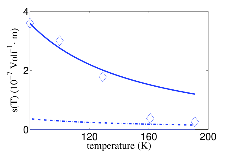
Figure 1: The slope $s(T)$ (see text) for a-Ge: diamonds are dataell . The dashed line is expected from the simple picture that the potential energy drops along the inverse direction of field for electronsbot ; fren . The solid line is calculated from (39). To estimate the average over various localized states, we take $\Delta G_{LL}=k_{B}T$.

The field polarizes the wave functions of occupied states and empty states (with a virtual positive charge). A static voltage on a sample adds a term to the double-well potential between two localized states:

$$U(y)=\frac{1}{2}ay^{2}+\frac{1}{4}by^{4}-eFy,$$ (40)

where $a\sim-k$ and $b\sim k/x_{0}^{2}$. To first order in the field, the two minima $y_{1}$ and $y_{2}$ of (40) do not shift. To second order in field, the distance between two minima of (40) decreases by an amount $\delta R=(3b/4a^{3})\sqrt{-a/b}(eF)^{2}$. This results in a further decrease of reorganization energymarcu in addition to the direct voltage drop.

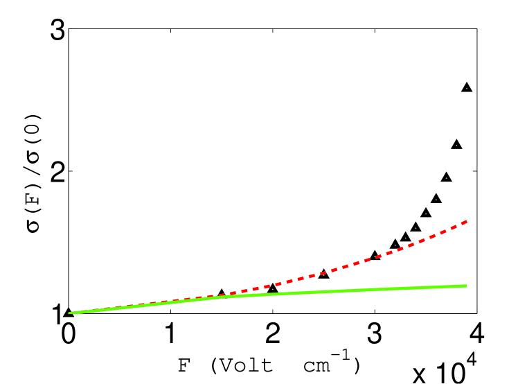
Figure 2: Field dependence of conductivity in vanadium oxide. The triangle symbols are measured rog values of $\sigma(F)/\sigma(F=0)$ for VO_1.83 at 200K. The solid line is the change in carrier density $n(E)/n(E=0)$ computed from Frenkel-Poole model, dashed line is the change in mobility $\mu(F)/\mu(F=0)$ from present work.

In Figure  2, we compare the observed $\sigma(F)/\sigma(F=0)$ resultsrog at 200K with the best fit of $\exp($const$\cdot F^{1/2})$ of the Frenkel-Poole model and with $\exp(s(T)F+dF^{2})$ of present work (VO_1.83 is of special interest for microbolometer applicationsrog ), where

$$d=(k_{B}T)^{-1}(Z^{\ast}e^{2}/4\pi\epsilon_{0}\epsilon_{s}R^{2})(3b/4a^{3})\sqrt{-a/b}e^{2}.$$

We can see from Figure 2 that the change in mobility provides a better description of experiments than that of the change in carrier density by field in the Frenkel-Poole modelfren .

3.4 Meyer-Neldel rule

From the formula for $\lambda_{LL}$ in the paragraph below (39), the reorganization energy for LL transitions decreases with rising temperature:

$$\delta\lambda_{LL}(T)=-4\delta T(1-T/T_{m})^{-1}T_{m}^{-1}\lambda_{LL}(T).$$

From (36),

$$\delta E_{a}^{LL}(T)=-E_{a}(0)\frac{\delta T}{T_{m}}(1-\frac{T}{T_{m}})^{-1}(1-\frac{\Delta G_{LL}^{2}}{\lambda_{LL}^{2}})\frac{\lambda_{LL}}{E_{a}^{LL}(0)}.$$ (41)

If $E_{a}^{LL}(T)$ decreases with rising temperature according to:

$$E_{a}^{LL}(T)=E_{a}^{LL}(0)(1-T/T_{MN}),$$ (42)

then the Meyer-Neldel rule is obtainedabt : comparing (41) and (42) one finds

$$T_{MN}\approx\frac{T_{m}}{4}(1+\frac{\Delta G_{LL}}{\lambda_{LL}})(1-\frac{\Delta G_{LL}}{\lambda_{LL}})^{-1}.$$ (43)

According to (35), during a LL transition the vibrational configurations of two localized tail states are reorganized. A large number of excitations (phonons) is required. A temperature-dependent activation energy implies that entropy must be involved and is an important ingredient for activation. The present approach supports the multi-excitation entropy theory of Yelon and MovagharYelon90 ; Yelon06 .

Table 1: predicted and observed Meyer-Neldel temperature T_MN in several materials (see text).

material	Tm(K)	$\epsilon_{s}$	d(Å)	$\xi/d$	$\Delta G_{LL}$(eV)	T${}_{MN}^{theory}$(K)	T${}_{MN}^{expt}$(K)
a-Si:H	1688	11.9	2.35	1.7-1.8	0.1	756-890	499-776Over
a-Ge1-xSe2Pbx	993	13	2.41	1.7	0.11	744	765eln
a-(As2Se3)100-x(SbSI)x	650	11	2.4	1.5	0.12	596	591sku
ZnO	2242	9.9-11	1.71	1.5	0.01	595	226-480schm ; sag
NiO	2257winch	11moni	1.75	1	0.06moni ; elp	1455	1460-1540dew

Table 1 is a comparison of the predicted Meyer-Neldel temperature $T_{MN}$ with observed ones. The number of atoms involved in a localized tail state is taken to the second nearest neighbor. The reorganization energy is estimated from the parameters given in Table 1, then T_MN is estimated from (43). Beside NiO, the most localized state extends to about $1.5d$. In NiO the hole of d electron shell is localized on one oxygen atom. The localization comes from the on-site repulsion in a d-band split by the crystal field. The theory agrees well with observations in quite different materials. In a typical ionic crystal like ZnO, the localized tail states arise from thermal disorder and are confined in very small energy range: $E_{U}\sim ku^{v2}/2\sim k_{B}T\sim 0.025$eV (T=300K). The fraction of localized carriers is much less than that in an amorphous semiconductor where localization is caused by static disorder. That is why $\Delta G_{LL}$ is about 10 times smaller than that in an amorphous semiconductor. In ZnO, most of the carriers are better described by large polarons. Taking the melting point as the localized-delocalized transition temperature $T_{m}$ is presumably an overestimation, so that the computed T_MN is too high.

3.5 Low temperatures

For low temperature ($k_{B}T\leq\hbar\bar{\omega}/10$), the argument in the last exponential of (34) is small. The exponential can be expanded in Taylor series and the ‘time’ integral can be completed. Denote:

$$f(\omega_{\alpha})=\frac{1}{2}(\theta_{\alpha}^{A_{3}}-\theta_{\alpha}^{A_{1}})^{2}csch\frac{\beta\hbar\omega_{\alpha}}{2},$$ (44)

then:

$$W_{T}(A_{1}\rightarrow A_{3})=\frac{2\pi J_{A_{3}A_{1}}^{2}}{\hbar}\exp\{\frac{-\beta\Delta G_{LL}^{0}}{2}\}$$

$$\exp\{-\frac{1}{2}\sum_{\alpha}(\theta_{\alpha}^{A_{3}}-\theta_{\alpha}^{A_{1}})^{2}\coth\frac{{}^{\beta\hbar\omega_{\alpha}}}{2}\}$$

$$\{\sum_{\alpha}f(\omega_{\alpha})\frac{1}{2}[\delta(\Delta G_{LL}^{0}+\hbar\omega_{\alpha})+\delta(\Delta G_{LL}^{0}-\hbar\omega_{\alpha})]$$

$$+\sum_{\alpha\alpha^{\prime}}f(\omega_{\alpha})f(\omega_{\alpha^{\prime}})\frac{1}{8}[\delta(\Delta G_{LL}^{0}+\hbar\omega_{\alpha}+\hbar\omega_{\alpha^{\prime}})$$

$$+\delta(\Delta G_{LL}^{0}-\hbar\omega_{\alpha}-\hbar\omega_{\alpha^{\prime}})$$

$$+\delta(\Delta G_{LL}^{0}+\hbar\omega_{\alpha}-\hbar\omega_{\alpha^{\prime}})+\delta(\Delta G_{LL}^{0}-\hbar\omega_{\alpha}+\hbar\omega_{\alpha^{\prime}})]\newline +\cdots\}.$$ (45)

One may say that the transfer integral is reduced by a factor $\exp\{-\frac{1}{4}\sum_{\alpha}(\theta_{\alpha}^{A_{3}}-\theta_{\alpha}^{A_{1}})^{2}\}$ due to the strong e-h coupling of localized states.

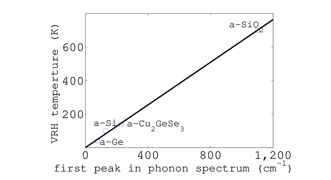
Figure 3: The present work predicts that the upper temperature limit of VRH is proportional to $\bar{\nu}$. The squares are observed data in several materialsbrod74 ; bah ; sriv ; awa ; oss ; gmar ; aiy , the line is a linear fit.

The derivation of (45) from (34) suggests that below a certain temperature T_up, the thermal vibrations of network do not have enough energy to adjust the atomic static displacements around localized states. The low temperature LL transition (45) becomes the only way to cause a transitions between two localized states (it does not need reorganization energy). Since the variable range hopping (VRH)motv is the most probable low temperature LL transition, T_up is the upper limit temperature of VRH.

On the other hand, the available thermal energy is $\sum_{j}\hbar\omega_{j}n_{j}$, where $n_{j}$ is the occupation number of the $j^{th}$ mode. At a low temperature, $n_{j}\sim exp(-\hbar\omega_{j}/k_{B}T)$, the available vibrational energy is determined by the number of modes with $\hbar\omega\leq k_{B}$T. The higher the frequency $\bar{\nu}$ of the first peak in phonon spectrum, the fewer the excited phonons. In other words, for a system with higher $\bar{\nu}$, only at higher temperature could one have enough vibrational energy to enable a transition. Therefore the present work predicts that for different materials, the upper temperature limit $T_{up}$ of VRH is proportional to the frequency $\bar{\nu}$ of the first peak in phonon spectrum.

Figure 3 reports experimental data for a-Sibrod74 , a-Gebrod74 ; bah , a-SiO₂sriv ; awa ; oss and a-Cu₂GeSe₃gmar ; aiy : the upper limit temperature T_up of VRH vs. the first peak of phonon spectrum $\bar{\nu}$. A linear relation between T_up and $\bar{\nu}$ is satisfied. From a linear fit, we deduce $T_{up}\approx\hbar\overline{\omega}/2.3k_{B}$, far beyond the more stringent condition T$<\hbar\overline{\omega}/10k_{B}$ for Taylor expansion of the exponential in (34). This is easy to understand: low frequency modes are acoustic, the density of states decreases quickly with reducing phonon frequency (Debye square distribution). T$<\hbar\overline{\omega}/10k_{B}$ is derived from csch$\frac{\beta\hbar\omega}{2}<0.01$ for all modes. The exponent of (34) is a summation over all modes. At $T_{up}\approx\hbar\overline{\omega}/2.3k_{B}$, although a single phonon seems have higher frequency, because the density of states at this frequency is small, the available vibration energy is low and VRH is already dominant.

4 Transition from a localized state to an extended state

The transition probability from localized state $A_{1}$ to extended state $B_{2}$ is:

$$W_{T}(A_{1}\rightarrow B_{2})=\frac{J_{B_{2}A_{1}}^{\prime 2}}{\hbar^{2}}e^{-\beta(E_{B_{2}}-E_{A_{1}}^{0}-\mathcal{E}_{A_{1}}^{b})/2}$$

$$\exp\{-\frac{1}{2}\sum_{\alpha}(\theta_{\alpha}^{A_{1}})^{2}\coth\frac{\beta\hbar\omega_{\alpha}}{2}\}\times$$

$$\int_{-t}^{t}d\tau\exp\{\frac{i\tau}{\hbar}(E_{B_{2}}-E_{A_{1}}^{0}-\mathcal{E}_{A_{1}}^{b})\}$$

$$[\exp\{\frac{1}{2}\sum_{\alpha}(\theta_{\alpha}^{A_{1}})^{2}csch\frac{\beta\hbar\omega_{\alpha}}{2}\cos\omega_{\alpha}\tau\}-1].$$ (46)

When a carrier moves out of a localized state, the nearby atoms are shifted and the occupation number in all modes are changed. Thus a LE transition is a multi-phonon process.

For ‘very’ high temperature $k_{B}T\geq 2.5\hbar\overline{\omega},$ (46) reduces to:

$$W_{T}^{LE}=\nu_{LE}e^{-E_{a}^{LE}/k_{B}T},~{}~{}E_{a}^{LE}=\frac{\lambda_{LE}}{4}(1+\frac{\Delta G_{LE}^{0}}{\lambda_{LE}})^{2},$$ (47)

where

$$\Delta G_{LE}^{0}=E_{B_{2}}-(E_{A_{1}}^{0}+\mathcal{E}_{A_{1}}^{b})$$ (48)

is the energy difference between extended state $B_{2}$ and localized state $A_{1}$, and

$$\nu_{LE}=\frac{J_{B_{2}A_{1}}^{\prime 2}}{\hbar}(\frac{\pi}{\lambda_{LE}k_{B}T})^{1/2},~{}\lambda_{LE}=\frac{1}{2}\sum_{\alpha}M_{\alpha}\omega_{\alpha}^{2}(\Theta_{\alpha}^{A_{1}})^{2}.$$ (49)

Here, $\lambda_{LE}$ is the reorganization energy for transition from localized state $A_{1}$ to extended state $B_{2}$. It is interesting to notice that the activation energy $E_{a}^{LE}$ for LE transition can be obtained by assuming $\Theta_{\alpha}^{A_{3}}=0$ in $\lambda_{LL}$. Transition from a localized state to an extended state corresponds to that of a particle escaping a barrier along the reaction pathkram .

Formally, the LE transition is similar to LL transition. To obtain the former, one makes the substitutions: $J_{A_{3}A_{1}}\rightarrow J_{B_{2}A_{1}}^{\prime}$, $\Theta_{\alpha}^{A_{3}}-\Theta_{\alpha}^{A_{1}}\rightarrow\Theta_{\alpha}^{A_{1}}$ and $[(E^{A_{1}}+\mathcal{E}_{b}^{A_{1}})-(E^{A_{3}}+\mathcal{E}_{b}^{A_{3}})]\rightarrow[E_{B_{2}}-(E_{A_{1}}^{0}+\mathcal{E}_{b}^{A_{1}})]$. However the physical meaning of the two are different.  From (37) and (49), we know that $\lambda_{LE}$ is the same order of magnitude as $\lambda_{LL}$. $\Delta G_{LE}^{0}$ is order of mobility edge, which is much larger than $\Delta G_{LL}^{0}$ and $J^{\prime}_{B_{2}A_{1}}>>J^{\prime}_{A_{3}A_{1}}$. The spatial displacement of the electron in a LE transition is about the linear size of the localized state.  From (47) and (36), $W_{T}^{LE}$ becomes comparable to $W_{T}^{LL}$ only when temperature is higher than $k_{B}^{-1}(E_{a}^{LE}-E_{a}^{LL})[2\ln(J_{LE}/J_{LL})]^{-1}$. The mobility edge of a-Si is about $0.1-0.2$eVbig ; yue , so that the LL transition is dominant in intrinsic a-Si below 580K. However if higher localized states close to the mobility edge are occupied due to doping, there exist some extended states which satisfy $\Delta G_{LE}^{0}\sim\Delta G_{LL}^{0}$. For these LE transitions, $E_{a}^{LE}$ is comparable to $E_{a}^{LL}$. The LE transition probability is about 10 times larger than that of LL transition. For these higher localized states, using parameters given for LL  transition in a-Si, $W_{T}^{LE}\sim 10^{13}$sec^-1.

According to approximation (i): $Y_{BA}<<1$ (Appendix A), (46) is only suitable for localized tail states which are far from the mobility edge. (46) complements Kikuchi’s idea of ‘phonon induced delocalization’kik : transitions from less localized states close to mobility edge to extended states. For less localized states, the coupling with atomic vibrations is weakerdra ; tafn , the reorganization energy $\lambda_{LE}$ is small. The transition from a less localized state (close to mobility edge) to an extended state is thus driven by single-phonon emission or absorptionkik , similar to the MA theorymil . Consider a localized state and an extended state, both close to the mobility edge. Then $\Delta G_{LE}^{0}$ is small, $W_{LE}$ can be large. The inelastic process makes the concept of localization meaningless for the states close to the mobility edgethou ; im .

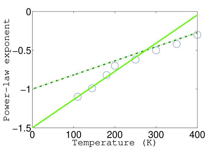
Figure 4: photocurrent time decay index as function of temperature: circles are data for a-Si:Hkris and a-As₂Se₃ore , dashed line is from the transition probability of MA theory, solid line is from (36,47) in $G<<\lambda$ limit. At higher temperature, $\lambda_{LE}\sim\Delta G_{LE}$, and the present result reduces to MA theory.

When a gap-energy pulse is applied to amorphous semiconductors, the transient photocurrent decays with a power-law: $t^{r(T)}$. The exponent is $r(T)=-1+k_{B}T/E_{U}$ according to a phenomenological MA type transition probability, $E_{U}$ is the Urbach energy of the band tailsch ; ore ; mon . (47) leads toHol2 $r(T)=-3/2+2k_{B}T/E_{U}$ if we follow the reasoning in ore ; mon ; bot . Figure 4 depicts the decay index as a function of temperature. At lower temperature the experimental data deviates from the prediction of the MA theory. At higher temperature and for states close to mobility edge, $\lambda\sim\Delta G$ and $E_{a}\sim\Delta G$, the present theory reduces to MA theorymon ; bot .

5 EL transition and EE transition

If an electron is initially in an extended state $|B_{1}\rangle$, the amplitude for a transition can be computed in perturbation theory. The probability of the transition from extended state $|B_{1}\rangle$ to localized state $|A_{2}\rangle$ is:

$$W_{T}(B_{1}\rightarrow A_{2})=\frac{1}{\hbar^{2}}\exp\{-\frac{\beta}{2}(E_{A_{2}}^{0}+\mathcal{E}_{A_{2}}^{b}-E_{B_{1}})\}$$

$$\exp\{-\frac{1}{2}\sum_{\alpha}(\theta_{\alpha}^{A_{2}})^{2}\coth\frac{\beta\hbar\omega_{\alpha}}{2}\}(I_{1}+I_{2}),$$ (50)

where:

$$I_{1}=\int_{-t}^{t}d\tau\exp\{\frac{i\tau}{\hbar}(E_{A_{2}}^{0}+\mathcal{E}_{A_{2}}^{b}-E_{B_{1}})\}$$

$$\exp\{\frac{1}{2}\sum_{\alpha}(\theta_{\alpha}^{A_{2}})^{2}csch\frac{\beta\hbar\omega_{\alpha}}{2}\cos\omega_{\alpha}\tau\}\times$$

$$[\sum_{\alpha^{\prime}}(\frac{1}{2}(K_{A_{2}B_{1}}^{\prime\alpha^{\prime}})^{2}+\frac{1}{4}(K_{A_{2}B_{1}}^{\prime\alpha^{\prime}}\theta_{\alpha^{\prime}}^{A_{2}})^{2}\coth\frac{\beta\hbar\omega_{\alpha^{\prime}}}{2})$$

$$\frac{\hbar}{M_{\alpha^{\prime}}\omega_{\alpha^{\prime}}}csch\frac{\beta\hbar\omega_{\alpha^{\prime}}}{2}\cos\omega_{\alpha^{\prime}}\tau$$

$$-\frac{1}{4}\sum_{\alpha^{\prime}}\frac{\hbar}{M_{\alpha^{\prime}}\omega_{\alpha^{\prime}}}(K_{A_{2}B_{1}}^{\prime\alpha^{\prime}}\theta_{\alpha^{\prime}}^{A_{2}})^{2}csch^{2}\frac{\beta\hbar\omega_{\alpha^{\prime}}}{2}\cos^{2}\omega_{\alpha^{\prime}}\tau],$$ (51)

and:

$$I_{2}=[\frac{1}{4}\sum_{\alpha^{\prime}}(K_{A_{2}B_{1}}^{\prime\alpha}\Theta_{\alpha^{\prime}}^{A_{2}})^{2}]\int_{-t}^{t}d\tau\exp\{\frac{i\tau}{\hbar}(E_{A_{2}}^{0}+\mathcal{E}_{A_{2}}^{b}-E_{B_{1}})\}\times$$

$$[\exp\{\frac{1}{2}\sum_{\alpha}(\theta_{\alpha}^{A_{2}})^{2}csch\frac{\beta\hbar\omega_{\alpha}}{2}\cos\omega_{\alpha}\tau\}-1].$$ (52)

For very high temperature $k_{B}T\geq 2.5\hbar\overline{\omega}$, the EL transition probability is

$$W_{EL}=\nu_{EL}e^{-E_{a}^{EL}/k_{B}T},$$ (53)

with

$$\nu_{EL}=\frac{1}{\hbar}(\frac{\pi}{k_{B}T\lambda_{EL}})^{1/2}\{\frac{1}{4}\sum_{\alpha^{\prime}}(K_{A_{2}B_{1}}^{\prime\alpha^{\prime}}\Theta_{\alpha^{\prime}}^{A_{2}})^{2}$$

$$+\sum_{\alpha^{\prime}}[\frac{(K_{A_{2}B_{1}}^{\prime\alpha^{\prime}})^{2}\hbar}{2M_{\alpha^{\prime}}\omega_{\alpha^{\prime}}}csch\frac{\beta\hbar\omega_{\alpha^{\prime}}}{2}+\frac{(K_{A_{2}B_{1}}^{\prime\alpha}\Theta_{\alpha^{\prime}}^{A_{2}})^{2}}{8}sech^{2}\frac{\beta\hbar\omega_{\alpha^{\prime}}}{4}]$$

$$-[2(\sum_{\alpha}\omega_{\alpha}^{2}(\theta_{\alpha}^{A_{2}})^{2}csch\frac{\beta\hbar\omega_{\alpha}}{2})^{-1}$$

$$-4\frac{(E_{A_{2}}^{0}+\mathcal{E}_{A_{2}}^{b}-E_{B_{1}})^{2}}{(\sum_{\alpha}\hbar\omega_{\alpha}^{2}(\theta_{\alpha}^{A_{2}})^{2}csch\frac{\beta\hbar\omega_{\alpha}}{2})^{2}}]\times$$

$$\times\sum_{\alpha^{\prime}}[\frac{(K_{A_{2}B_{1}}^{\prime\alpha^{\prime}})^{2}\hbar\omega_{\alpha^{\prime}}}{4M_{\alpha^{\prime}}}csch\frac{\beta\hbar\omega_{\alpha^{\prime}}}{2}$$

$$+\frac{\omega_{\alpha^{\prime}}^{2}(K_{A_{2}B_{1}}^{\prime\alpha^{\prime}}\Theta_{\alpha^{\prime}}^{A_{2}})^{2}\coth\frac{\beta\hbar\omega_{\alpha^{\prime}}}{2}}{8}csch\frac{\beta\hbar\omega_{\alpha^{\prime}}}{2}$$

$$-\frac{\omega_{\alpha^{\prime}}^{2}(K_{A_{2}B_{1}}^{\prime\alpha^{\prime}}\Theta_{\alpha^{\prime}}^{A_{2}})^{2}}{4}csch^{2}\frac{\beta\hbar\omega_{\alpha^{\prime}}}{2}]\},$$ (54)

and

$$E_{a}^{EL}=\frac{\lambda_{EL}}{4}(1+\frac{\Delta G_{EL}^{0}}{\lambda_{EL}})^{2},~{}~{}\lambda_{EL}=\frac{1}{2}\sum_{\alpha}M_{\alpha}\omega_{\alpha}^{2}(\Theta_{\alpha}^{A_{2}})^{2},$$

$$\Delta G_{EL}^{0}=E_{A_{2}}^{0}+\mathcal{E}_{A_{2}}^{b}-E_{B_{1}}<0,$$ (55)

where $\lambda_{EL}$ is order of magnitude of $\lambda_{LL}$. Because $\Delta G_{EL}^{0}<0$, from the expressions of $E^{EL}_{a}$ and $E^{LL}_{a}$, we know $E_{a}^{EL}$ is smaller than $E_{a}^{LL}$. Since $K_{A_{2}B_{1}}^{\prime\alpha^{\prime}}\Theta_{\alpha^{\prime}}^{A_{2}}$ is the same order magnitude as $J_{A_{3}A_{1}}$, the EL transition probability is larger than that of LL transition. In a-Si, this yields $W_{T}^{EL}\sim 10^{13}-10^{14}$sec^-1. When a carrier moves in a localized state, the nearby atoms are shifted due to the e-ph interaction, so that all modes are affected. Thus an EL transition is a multi-phonon process.

$\Delta G_{EL}^{0}<0$ has a deep consequence. From the expression (24) for $\mathcal{E}_{A_{2}}^{b}$ and the order of magnitude of mobility edgesca , we know that the energy difference $\Delta G_{EL}^{0}<0$ is order several tenths eV. For extended states with $|\Delta G_{EL}^{0}|/\lambda_{EL}<1$, we are in the normal regime: the higher the energy of an extended state (i.e. $\Delta G_{EL}^{0}/\lambda_{EL}$ more negative but still $|\Delta G_{EL}^{0}|/\lambda_{EL}<1$), the smaller the activation energy $E_{a}^{EL}$. The higher extended state has a shorter lifetime, therefore the time that an electron is able to remain in such an extended state is less than the time it spends in a lower extended state. An extended state with shorter lifetime contributes less to the conductivity. For extended states with energies well above the mobility edge (such that $|\Delta G_{EL}^{0}|/\lambda_{EL}>1$), we are in Marcus inverted regime (cf. Figure 5): the higher the energy of an extended state, the larger the activation energy. The higher extended states have long lifetimes and will contribute more to conductivity. In the middle of the two regimes, $\Delta G_{EL}^{0}/\lambda_{EL}\approx-1$. For these extended states, no activation energy is required for the transition to localized states. Such extended states will quickly decay to the localized states. In experiments, there is indirect evidence for the existence of this short-lifetime belt. In a crystal, phonon-assisted non-radiative transitions are slowed by the energy-momentum conservation law. In c-Si/SiO₂ quantum well structure, the photoluminescence lifetime is about 1 ms, and is insensitive to the wavelengthoka . The photoluminescence lifetime of a-Si/SiO₂ structure becomes shorter with a decrease in wavelength: 13ns at 550nm and 143ns at 750nmkan . The trend is consistent with the left half of Figure 5. The observed wavelength indicates that the energy difference ($>1.66$eV) between the hole and electron is larger than band gap (1.2eV), so that the excited electrons are in extended states. According to (54) and Figure 5, higher extended states are more quickly depleted by the non-radiative transitions than the lower ones, so that a photoluminescence signal with higher frequency has a shorter lifetime. We need to be careful on two points: (i) the observed recombination time is order of ns, it is the EE transitions that limits EL transition to a large extent; (ii) for a quantum well, the number of atoms is small, so that the reorganization energy is smaller than the bulk. The static displacements may be able to adjust at the experiment temperature 2-10K. To really prove the existence of the short-lifetime belt, one needs to excite electrons into and above the belt with two narrow pulses: if the higher energy luminescence lasts longer than the lower energy one, the existence of a short-lifetime belt is demonstrated.

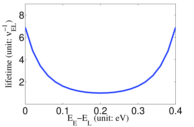
Figure 5: The non-radiative transition lifetime of extended state as function of energy difference $E_{E}-E_{L}$ between initial extended state and final localized state. $\lambda_{EL}=0.2$ eV is estimated from the data given in Sec. III. When $E_{E}-E_{L}=\lambda_{EL}$, lifetime is a minimum. The short lifetime belt exists in range 0.1 eV$<E_{E}-E_{L}<0.3$eV. The vertical axis is scaled by $\nu_{EL}^{-1}$.

In the conduction band, the energy of any localized tail state is lower than that of any extended state, so that a zero-phonon process is impossible. Because the $\Delta G_{EL}^{0}<0,$ factor $\exp[|\Delta G_{EL}^{0}|/(2k_{B}T)]$ increases with decreasing temperature. On the other hand, other factors in (63) decrease with decreasing temperature. Thus there exists an optimal temperature T_∗, at which the transition probability is maximum. If one measures the variation of luminescence changing with temperature in low temperature region, at T_∗ the lifetime of the photoluminescence will be shortest.

A transition from one extended state to another extended state is a single-phonon absorption or emission process driven by e-ph interaction. The transition probability from extended state $|B_{1}\rangle$ to extended state $|B_{2}\rangle$ is:

$$W(B_{1}\rightarrow B_{2})=\frac{2\pi}{\hbar}\sum_{\alpha^{\prime}}(K_{B_{2}B_{1}}^{\alpha^{\prime}})^{2}\frac{\hbar}{M_{\alpha^{\prime}}\omega_{\alpha^{\prime}}}$$

$$[\frac{\overline{N_{\alpha^{\prime}}^{\prime}}}{2}\delta(E_{B_{2}}-E_{B_{1}}-\hbar\omega_{\alpha^{\prime}})+\frac{\overline{N_{\alpha^{\prime}}^{\prime}}+1}{2}\delta(E_{B_{2}}-E_{B_{1}}+\hbar\omega_{\alpha^{\prime}})],$$ (56)

where $\overline{N_{\alpha^{\prime}}^{\prime}}=(e^{\beta\hbar\omega_{\alpha^{\prime}}}-1)^{-1}$ is the average phonon number in the $\alpha^{\prime}$th mode. In a crystal, (56) arises from inelastic scattering with phonons.

5.1 Four transitions and conduction mechanisms

Table 2: Some features of 4 types of transitions in a-Si.

transitions	origin	phonons needed	activated	role in conduction	probability $W_{T}$(sec-1)
L$\rightarrow$L	$J$ (9)	multi	yes	direct	$10^{12}$
L$\rightarrow$E	$J^{{}^{\prime}}$ (11)	multi	yes	direct+indirect	$10^{10}-10^{13}$
E$\rightarrow$L	$K^{{}^{\prime}}$ (10)	multi	yes	direct+indirect	$10^{13}-10^{14}$
E$\rightarrow$E	$K$ (12)	single	no	reduce	$10^{13}$

The characteristics of the four types of transitions are summarized in Table 2. The last column gives the order of magnitude of the transition probability estimated from the parameters of a-Si at T=300K. In a-Si:H, the role of hydrogen atoms is to passivate dangling bond, the estimated rates are roughly applicable to a-Si:H. The rate of LL transitions is between two nearest neighbors. For an intrinsic or lightly n-doped semiconductor at moderate temperature (for a-Si $T<580$K, the energy of mobility edge), only the lower part of conduction tail is occupied. Then $\Delta G_{LE}$ is large, and the LE transition probability is about two orders of magnitude smaller than that of the LL transition. For an intrinsic semiconductor at higher temperature or a doped material, $\Delta G_{LE}^{0}$ becomes comparable to $\Delta G_{LL}^{0}$, LE transition probability is about ten times larger than that of LL transition. The first three transitions increase the mobility of an electron, whereas EE transition decreases mobility of an electron.

Although $W_{EL}>W_{LE}$, the transient decay of photocurrent is still observableore . The reason is that for extended states below the short-lifetime belt, $W_{EL}\sim W_{EE}$, so that an electron in an extended state can be scattered into another extended state and continue to contribute to conductivity before becoming trapped in some localized state.

If a localized tail state is close to the bottom of the conduction band, for another well localized state and an extended state close to mobility edge, $\Delta G_{LE}\sim\Delta G_{LL}+D$, and $W_{LE}$ is one or two orders of magnitude smaller than $W_{LL}$. If a localized state is close to mobility edge, $\Delta G_{LE}\sim\Delta G_{LL},$ because $J^{\prime}$ is several times larger than $J,$ $W_{LE}$ could be one order of magnitude larger than $W_{LL}$. The probability of EL transition is then one or two orders of magnitude larger than that of LL transition. The reason is that $\Delta G_{EL}<0$, $E_{a}^{EL}$ is smaller than $E_{a}^{LL}$ while $K^{\prime}\Theta$ is the same order of magnitude as $J$. The probability of EE transition $W_{EE}$ is about 10³ times larger than $W_{LL}$ (cf. Table 2). The EE transition deflects the drift motion which is along the direction of electric field and reduces conductivity. This is in contrast with the LL, LE and EL transitions. The relative contribution to conductivity of four transitions also depends on the number of carriers in extended states and in localized states, which are determined by the extent of doping and temperature. At low temperature ( $k_{B}T<\hbar\overline{\omega}/10$), the non-diagonal transition is still multi-phonon activated process whatever it is LL, LE or EL transition. The activation energy is just half of the energy difference between final state and initial state (cf. (37), (48) and (55)).

5.2 Long time and higher order processes

The perturbation treatments of the four fundamental processes are only suitable for short times, in which the probability amplitude of the final state is small. Starting from a localized state we only have $L\rightarrow E$ process and $L\rightarrow L$ process. Starting from an extended state, we only have $E\rightarrow L$ process and $E\rightarrow E$ process. For long times, higher order processes appear. For example $L\rightarrow E\rightarrow L\rightarrow L\rightarrow E\rightarrow L\rightarrow E\rightarrow E\rightarrow L$ etc. Those processes are important in amorphous solids. In a macroscopic sample, there are many occupied localized and extended states. If we are concerned with the collective behavior of all carriers rather than an individual carrier in a long time period, the picture of the four transitions works well statistically.

All four transitions are important to dc conductivity and transient photocurrent. In previous phenomenological models, the role of LE transition was taken into account by parameterizing the MA probabilityore ; mon . The details of LE transition and the polarization of network by the localized carriers were ignored. The present work has attempted to treat the four transitions in a unified way. Our approach enhanced previous theories in two aspects: (1) the role of polarization is properly taken into account; and (2) we found the important role played by the EL transition and associated EE transition in dc conductivity and in the non-radiative decay of extended states.

6 Summary

For amorphous solids, we established the evolution equations for localized tail states and extended states in the presence of lattice vibrations. For short times, perturbation theory can be used to solve Eqs.(6) and (7). The transition probabilities of LL, LE, EL and EE transitions are obtained. The relative rates for different processes and the corresponding control parameters are estimated.

The new results found in this work are summarized in the following. At high temperature, any transition involving well-localized state(s) is a multi-phonon process, the transition rate takes form (1). At low temperature, variable range hopping appears as the most probable LL transitions.

The field-dependence of the conductivity estimated from LL transition is closer to experiments than previous theories. The predicted Meyer-Neldel temperature and the linear relation between the upper temperature limit of VRH and the frequency $\bar{\nu}$ of first peak of phonon spectrum are consistent with experiments in quite different materials.

We suggested that there exists a short lifetime belt of extended states inside conduction band or valence band. These states favor non-radiative transitions by emitting several phonons.

From (59) one can see that single-phonon LL transition appears when states become less localized. In intrinsic or lightly doped amorphous semiconductors, the well localized states are the low lying excited states and are important for transport. Carriers in these well localized tail states polarize the network: any process involving occupation changes of well localized tail states must change the occupation numbers in many vibrational modes and are multi-phonon process. Moving towards to the mobility edge, the localization length of a state becomes larger and larger. When the static displacements caused by the carrier in a less localized state are comparable to the vibrational displacements, one can no longer neglected the vibrational displacements in (59). The usual electron-phonon interaction also plays a role in causing transition from a less localized state. In this work, we did not discuss this complicated situation. Formally when reorganization energy $\lambda_{LL}$ between two localized states is small and comparable to the typical energy difference $\Delta G_{LL}$, the present multi-phonon LL transition probability reduces to single-photon MA theory.

The multi-phonon LE transition discussed in this work is for well localized states, it is a supplement to the theory of phonon-induced delocalization which is concerned with the less localized states close to the mobility edge. As discussed in Appendix A, when the atomic static displacements caused by a carrier in a less localized state is comparable to the vibrational amplitude, LE transition could be caused either by a phonon in resonance with the initial and final states or by the transfer integral $J^{{}^{\prime}}_{B_{2}A_{1}}$.

Appendix A Approximations used to derive evolution equations

Usually in the zero order approximation of crystals (specially in the theory of metals), the full potential energy
$\sum_{\mathbf{n}}U_{\mathbf{n}}(r-\mathbf{R}_{\mathbf{n}}-\mathbf{u}_{v}^{\mathbf{n}})$ is replaced by $V_{c}=\sum_{\mathbf{n}}U_{\mathbf{n}}(r-\mathbf{R}_{\mathbf{n}})$, where $\mathbf{R}_{\mathbf{n}}$ and $\mathbf{u}_{v}^{\mathbf{n}}$ are the equilibrium position and vibrational displacemet of the $n$th atom. One then diagonalizes $h_{c}=-\hbar^{2}\nabla^{2}/2m+V_{c}$, such that all eigenstates are orthogonal. Electron-phonon interaction $\sum_{j=1}^{3\mathcal{N}}x_{j}\frac{\partial U}{\partial X_{j}}$ slightly modifies the eigenstates and eigenvalues of $h_{c}$ or causes scattering between eigenstates. This procedure works if e-ph interaction does not fundamentally change the nature of Bloch states. As long as static disorder is not strong enough to cause localization, Bloch states are still proper zero order states. However one should be careful when dealing with the effect of static disorder $\{\mathbf{u}_{s}^{\mathbf{n}}\}$. It must be treated as perturbation along with e-ph interaction. If we put static disorder in potential energy and diagonalize $h_{s}=-\hbar^{2}\nabla^{2}/2m+\sum_{\mathbf{n}}U_{\mathbf{n}}(r-\mathbf{R}_{\mathbf{n}}-\mathbf{u}_{s}^{\mathbf{n}})$, the scattering effect of static disorder disappear in the disorder-dressed eigenstates. The physical properties caused by static disorder e.g. resistivity is not easy to display in an intuitive kinetic consideration based on Boltzmann-like equation: eigenstates of $h_{s}$ are not affected by static disorder $\{\mathbf{u}_{s}^{\mathbf{n}}\}$. By contrast, computing transport coefficients with eigen states of $h_{s}$ is not a problem in Kubo formula or its improvmentkubo .

We face a dilemma in amorphous semiconductors. On one hand the static disorder $\{\mathbf{u}_{s}^{\mathbf{n}}\}$ is so strong that some band tail states are localized, static disorder must be taken into account at zero order i.e. diagonalize $h_{s}$; on the other hand from kinetic point-of-view the carriers in extended states are scattered by the static disorder which should be displayed explicitly $\sum_{\mathbf{n}}\mathbf{u}_{s}^{\mathbf{n}}\cdot\partial U_{\mathbf{n}}(r-\mathbf{R}_{\mathbf{n}})/\partial\mathbf{R}_{\mathbf{n}}$ rather than included in the exact eigenstates of $h_{s}$.

The very different strengths of the e-ph interaction in localized states and in extended states also requires different partitions of the potential energy $\sum_{\mathbf{n}}U_{\mathbf{n}}(r-\mathcal{R}_{\mathbf{n}}-\mathbf{u}_{v}^{\mathbf{n}})$, where $\mathcal{R}_{\mathbf{n}}=\mathbf{R}_{\mathbf{n}}+\mathbf{u}_{s}^{\mathbf{n}}$ is the static position of the $n^{th}$ atom in an amorphous solid. Molecular dynamics (MD) simulationsdra ; tafn show that the eigenvalues of localized states are strongly modified (about several tenth eV) by e-ph interaction, while the eigenvalues of extended states do not fluctuate much. It seems reasonable that for localized states we should include e-ph interaction at zero order, and put it in the zero-order single-particle potential energy (just like small polaron theoryHol1 ; Hol2 ), while for extended states e-ph interaction acts like a perturbation (similar to the inelastic scattering of electrons caused by e-ph interaction in metals).

The traditional partition of full potential energy is

$$\sum_{\mathbf{n}}U(r-\mathcal{R}_{\mathbf{n}},\mathbf{u}^{\mathbf{n}})=\sum_{\mathbf{n}=1}^{\mathcal{N}}U(\mathbf{r}-\mathcal{R}_{\mathbf{n}})+\sum_{j=1}^{3\mathcal{N}}x_{j}\frac{\partial U}{\partial X_{j}}.$$ (57)

In this ansatz, static disorder is included at zero order. Localized states and extended states are eigen states of $h_{s}$. The second term of (57), the e-ph interaction, is the unique residual perturbation to eigenstates of $h_{s}$. It causes transitions among the eigen states of $h_{s}$ i.e. LL, LE, EL and EE transitions, to lowest order transition is driven by single-phonon absorption or emission. Since all attractions due to static atoms are included in $h_{s}$, two types of transfer integrals $J_{A_{2}A_{1}}$ (from a localized state to another localized state) and $J_{B_{2}A_{1}}^{\prime}$ (from a localized state to an extended state) do not exist. One can still use Kubo formula or subsequent developmentkubo to compute transport coefficients.

However partition (57) obscures the construction of a
Boltzmann-like picture for electronic conduction where various agitation and obstacle mechanisms are explicitly exposed. The elastic scattering caused by static disorder is hidden in the eigen states of $h_{s}$. To explicitly illustrate the elastic scattering produced by static disorder, one has to further resolve the first term of (57) into

$$\sum_{\mathbf{n}=1}^{\mathcal{N}}U(\mathbf{r}-\mathcal{R}_{\mathbf{n}})=\sum_{\mathbf{n}=1}^{\mathcal{N}}U(\mathbf{r}-\mathbf{R}_{\mathbf{n}})$$

$$+\sum_{\mathbf{n}}\mathbf{u}_{s}^{\mathbf{n}}\cdot\partial U_{\mathbf{n}}(r-\mathbf{R}_{\mathbf{n}})/\partial\mathbf{R}_{\mathbf{n}}.$$ (58)

(57) is also inconvenient for localized states. The e-ph interaction for a carrier in a localized state is much stronger than in an extended statedra ; tafn . It is reflected in two aspects: (i) a localized carrier polarizes network and produces static displacements for the atoms in which the localized state spread; (ii) the wave functions and corresponding eigenvalues of localized states are obviously changed (the change in eigenvalues can be clearly seen in MD trajectorydra ; tafn ). To describe these two effects, in perturbation theory one has to calculate e-ph interaction to infinite order.

Taking different partitions for localized states and extended states is a practical ansatz.For a localized state, we separate

$$\sum_{\mathbf{n}}U(r-\mathcal{R}_{\mathbf{n}},\mathbf{u}_{v}^{\mathbf{n}})=\sum_{\mathbf{n}\in D_{A_{1}}}U(r-\mathcal{R}_{\mathbf{n}},\mathbf{u}_{v}^{\mathbf{n}})$$

$$+\sum_{\mathbf{p}\notin D_{A_{1}}}U(r-\mathcal{R}_{\mathbf{p}},\mathbf{u}_{v}^{\mathbf{p}}),$$ (59)

where $D_{A_{1}}$ is the distorted region where localized tail state $\phi_{A_{1}}$ spreads. For a nucleus outside $D_{A_{1}}$, its effect on localized state $A_{1}$ dies away with the distance between the nucleus and $D_{A_{1}}$. The second term leads to two transfer integrals $J_{A_{2}A_{1}}$ (induces LL transition) and $J_{B_{2}A_{1}}^{\prime}$ (induces LE transition) in the evolution equations of localized states.

Since for a well-localized state $\phi_{A_{1}}$, the wave function is only spread on the atoms in a limited spatial region $D_{A_{1}}$, $\langle\phi_{A_{1}}|\cdot|\phi_{A_{1}}\rangle=0$, where $\cdot$ stands for the second term in the RHS of (59). In calculating $J_{A_{2}A_{1}}=\langle\phi_{A_{2}}|\cdot|\phi_{A_{1}}\rangle$ and $J_{B_{2}A_{1}}^{\prime}=\langle\xi_{B_{2}}|\cdot|\phi_{A_{1}}\rangle$, it is legitimate to neglect $\mathbf{u}_{v}^{\mathbf{p}}$, $\cdot\thickapprox\sum_{\mathbf{p}\notin D_{A_{1}}}U(r-\mathcal{R}_{\mathbf{p}})$. The change in potential energy induced by the atomic vibrational displacements is fully included in the first term in RHS of (59). Because the wave function $\phi_{A_{1}}$ of localized state $A_{1}$ is confined in $D_{A_{1}}$, one can view $\phi_{A_{1}}$ as the eigenfunction of $h_{A_{1}}^{0}=-\hbar^{2}\nabla^{2}/2m+\sum_{\mathbf{n}\in D_{A_{1}}}U(r-\mathcal{R}_{\mathbf{n}},\mathbf{u}_{v}^{\mathbf{n}})$ with eigenvalue $E_{A_{1}}(\{\mathbf{u}_{v}^{\mathbf{n}},\mathbf{n}\in D_{A_{1}}\})$. The rest of atoms outside $D_{A_{1}}$ act as boundary of $\phi_{A_{1}}$. A carrier in localized state $\phi_{A_{1}}$ propagates in region $D_{A_{1}}$ and is reflected back at the boundary of $D_{A_{1}}$.Since static disorder is fully contained in $h_{A_{1}}^{0}$, in the present ansatz, localized carriers are free from elastic scattering of static disorder.

For a less localized state $\phi_{A_{1}}$, its wave function spreads over a wider spatial region $D_{A_{1}}$. With shift to the mobility edge, $\sum_{\mathbf{n\in}D_{A_{1}}}\mathbf{u}_{v}^{\mathbf{n}}\cdot\nabla U(r-\mathcal{R}_{\mathbf{n}})$ become smaller and smaller, eventually comparable to $\sum_{\mathbf{p}\notin D_{A_{1}}}U(r-\mathcal{R}_{\mathbf{p}})$ and $\sum_{\mathbf{p}\notin D_{A_{1}}}\mathbf{u}_{v}^{\mathbf{p}}\cdot\nabla U(r-\mathcal{R}_{\mathbf{p}},\mathbf{u}_{v}^{\mathbf{p}})$. For carriers on these less localized states, their polarization of the network is weak, and the atomic static displacements are comparable to the vibrational amplitudes. Entering or leaving a less localized state does not require configuration reorganization, and the reorganization energy becomes same order of magnitude as vibrational energy. For such a situation, only a phonon in resonance with the initial and final states contributes to the transition. The multi-phonon processes gradually become the single-phonon processes, although the driving force is still the transfer integral induced by $\sum_{\mathbf{p}\notin D_{A_{1}}}U(r-\mathcal{R}_{\mathbf{p}})$. One obtains the MA theory.

For a less localized state, if we treat $\sum_{\mathbf{n\in}D_{A_{1}}}\mathbf{u}_{v}^{\mathbf{n}}\cdot\nabla U(r-\mathcal{R}_{\mathbf{n}})$, $\sum_{\mathbf{p}\notin D_{A_{1}}}U(r-\mathcal{R}_{\mathbf{p}})$ and $\sum_{\mathbf{p}\notin D_{A_{1}}}\mathbf{u}_{v}^{\mathbf{p}}\cdot\nabla U(r-\mathcal{R}_{\mathbf{p}},\mathbf{u}_{v}^{\mathbf{p}})$ in the same foot as perturbation, the phonon-induced delocalization naturally appears and is accompany with EL transitions induced by transfer integral $J^{{}^{\prime}}_{B_{2}A_{1}}$.

For extended states, to construct a kinetic description, (57) is suitable partition of full potential energy. The second term of (57), the e-ph interaction, causes EL and EE transitions in the evolution equation of extended state. The elastic scattering of the carriers in extended states induced by static disorder can be taken into account by two methods: (i) Using the eigenvalues and eigenfunctions of $h_{s}$ in Kubo formula; (2) if we wish to deal static disorder more explicitly, we can apply coherent potential approximation to (58). In this work we do not discuss these issues and only concentrate on the transitions involving atomic vibrations.

In deriving (6,7), we neglected the dependence of extended state $\xi_{B_{1}}$ on the vibrational displacements, then $\nabla_{j}\xi_{B_{1}}=0$. Since $v_{n}/v_{e}\sim 10^{-3}$ (where $v_{e}$ and $v_{n}$ are typical velocities of the electron and nucleus), $m/M\sim 10^{-4}$ ($m$ and $M$ are mass of electron and of a typical nucleus) and $x/d\sim 10^{-2}-10^{-1}$ ($x$ and $d$ are typical vibrational displacement of atom and bond length), one can show $\sum_{j}(\hbar^{2}/M_{j})(\nabla_{j}a_{A_{1}})(\nabla_{j}\phi_{A_{1}})$ or $\sum_{j}(\hbar^{2}/2M_{j})\nabla_{j}^{2}\phi_{A_{1}}<<\sum_{\mathbf{p}\notin D_{A_{1}}}U(r-\mathcal{R}_{\mathbf{p}},\mathbf{u}^{\mathbf{p}})\phi_{A_{1}}$ or $\sum_{j}x_{j}(\partial U/\partial X_{j})\xi_{B_{1}}$. Therefore terms including $\nabla_{j}\phi_{A_{1}}$ or  $\nabla_{j}^{2}\phi_{A_{1}}$ can be neglected.

To further simplify the evolution equations, we need two connected technical assumptions: (i) the overlap integral $Y_{B_{2}A_{1}}$ between extended state $\xi_{B_{2}}$ and localized tail state $\phi_{A_{1}}$ satisfies $Y_{B_{2}A_{1}}\sim N_{A_{1}}/\mathcal{N}<<1$ and (ii) overlap integral $S_{A_{2}A_{1}}$ between two localized tail states satisfies $S_{A_{2}A_{1}}<<1$. Assumption (i) means that we do not consider the localized tail states very close to the mobility edge and consider only the most localized tail states. Condition (ii) is satisfied for two localized states which do not overlap. It means we exclude the indirect contribution to conductivity from the transitions between two localized tail states with overlapping spatial regions.

For two localized states $A_{2}$ and $A_{1}$, $S_{A_{2}A_{1}}<<1$ if $D_{A_{1}}$ and $D_{A_{2}}$ do not overlap. The terms multiplied by $S_{A_{2}A_{1}}$ can be neglected for localized tail states which their spatial regions do not overlap. What is more, the transfer integral is important only when the atoms $\mathbf{p}\notin D_{A_{1}}$ fall into $D_{A_{2}}$ or $A_{1}=A_{2}$,

$$\sum_{A_{1}}a_{A_{1}}\int d^{3}r\phi_{A_{2}}^{\ast}\sum_{\mathbf{p}\notin D_{A_{1}}}U(r-\mathcal{R}_{\mathbf{p}},\mathbf{u}^{\mathbf{p}})\phi_{A_{1}}$$

$$\approx\sum_{A_{1}}a_{A_{1}}J_{A_{2}A_{1}}+W_{A_{2}}a_{A_{2}}$$ (60)

where $W_{A_{2}}=\int d^{3}r|\phi_{A_{2}}|^{2}\sum_{\mathbf{p}\notin D_{A_{2}}}U(r-\mathcal{R}_{\mathbf{p}},\mathbf{u}^{\mathbf{p}})$ only affects the self energy of a localized state through $a_{A_{2}}$. Comparing with $E_{A_{1}}$ and with $h_{v}$, $W_{A_{2}}$ can be neglectedHol1 .

Appendix B Scales of the coupling parameters of four transitions

For these most localized tail states, the wave functions take the form of $\phi_{A_{1}}\sim e^{-|\mathbf{r}-\mathcal{R}_{A_{1}}|/\xi_{1}}$. $J_{A_{2}A_{1}}$ is estimated to be $-(N_{A_{2}}Z^{\ast}e^{2}/4\pi\epsilon_{0}\varepsilon_{s}\xi)(1+R_{12}/\xi)e^{-R_{12}/\xi}$, where average localization length $\xi$ is defined by $2\xi^{-1}=\xi_{1}^{-1}+\xi_{2}^{-1}$. $R_{12}$ is the average distance between two localized states, $\varepsilon_{s}$ is the static dielectric constant, $Z^{\ast}$ is the effective nuclear charge of atom, $N_{A_{2}}$ is the number of atoms inside region $D_{A_{2}}$. Later we neglect the dependence of $J_{A_{2}A_{1}}$ on the vibrational displacements $\{x\}$ of the atoms and consider $J_{A_{2}A_{1}}$ as a function of the distance $R_{12}$ between two localized states, localization length $\xi_{1}$ of state $\phi_{A_{1}}$ and localization length $\xi_{2}$ of state $\phi_{A_{2}}$. If a localized state is not very close to the mobility edge, its localization length $\xi$ is small. The overlap between it and an extended state $Y_{B_{2}A_{1}}\sim N_{A_{1}}/\mathcal{N}$ may be neglected.

If we approximate extended states as plane waves $\xi_{B_{1}}\sim e^{ik_{B_{1}}r}$, then $K_{A_{2}B_{1}}^{\prime}\sim(Z^{\ast}e^{2}u/4\pi\epsilon_{0}\varepsilon_{s}\xi_{A_{2}}^{2})(1-ik_{B_{1}}\xi_{A_{2}})^{-1}$. So that $K_{A_{2}B_{1}}^{\prime}u/J_{A_{2}A_{1}}\sim e^{R_{12}/\xi}u/\xi$, where $u\sim\\ \sqrt{k_{B}T/M\omega^{2}}$ or $\sqrt{\hbar/M\omega}$ is typical amplitude of vibration at high or low temperature. The distance between two nearest localized states is $\sim$ several Å in a-Si, and $K_{A_{2}B_{1}}^{\prime}u$ is several times smaller than $J_{A_{2}A_{1}}$. If we again approximate extended state as plane wave $\xi_{B_{2}}^{\ast}\sim e^{-ik_{B_{2}}r}$, $J_{B_{2}A_{1}}^{\prime}\sim(Z^{\ast}e^{2}/4\pi\epsilon_{0}\varepsilon_{s}\xi_{A_{1}})(1+ik_{B_{2}}\xi_{A_{1}})^{-2}$. $J_{B_{2}A_{1}}^{\prime}$ is of the same order of magnitude as $J_{A_{2}A_{1}}$. $J_{B_{2}A_{1}}^{\prime}$ does not create transitions from an extended state to a localized state. The asymmetries in (10) and (11) come from the different separations (59) and (58) of the single particle potential energy for localized states and extended states. One should not confuse this with the usual symmetry between transition probabilities for forward process and backward process computed by the first order perturbation theory, where two processes are coupled by the same interaction. If we approximate extended states $\xi_{B_{1}}$ and $\xi_{B_{2}}$ by plane waves with wave vector $k_{1}$ and $k_{2}$, $K_{B_{2}B_{1}}\sim Z^{\ast}e^{2}u\kappa^{3}/(4\pi\epsilon_{0}\varepsilon_{s}[\kappa+i(k_{2}-k_{1})])$, where $\kappa\sim(e^{2}/\epsilon_{0})(\partial n/\partial\mu)$ is the Thomas-Fermi screening wave vector. In a lightly doped or intrinsic semiconductor, $\kappa$ is hundreds or even thousands times smaller than $1/a,$ $a$ is bond length. Since for most localized state, localization length $\xi$ is several times $a$, therefore $K_{B_{2}B_{1}}\sim(\kappa\xi)^{2}K_{A_{2}B_{1}}^{\prime}$, is much weaker than three other coupling constants.

Appendix C LE transition at low temperature

The LE transition probability for low temperature $k_{B}T\leq\hbar\overline{\omega}/10$ can be worked out as in (45). Denote:

$$f_{LE}(\omega_{\alpha})=\frac{1}{2}(\theta_{\alpha}^{A_{1}})^{2}csch\frac{\beta\hbar\omega_{\alpha}}{2},$$ (61)

and the result is

$$W_{T}(A_{1}\rightarrow B_{2})=\frac{2\pi J_{B_{2}A_{1}}^{\prime 2}}{\hbar}\exp\{\frac{-\beta\Delta G_{LE}^{0}}{2}\}$$

$$\exp\{-\frac{1}{2}\sum_{\alpha}(\theta_{\alpha}^{A_{1}})^{2}\coth\frac{{}^{\beta\hbar\omega_{\alpha}}}{2}\}\times$$

$$\{\sum_{\alpha}f_{LE}(\omega_{\alpha})\frac{1}{2}[\delta(\Delta G_{LE}^{0}+\hbar\omega_{\alpha})+\delta(\Delta G_{LE}^{0}-\hbar\omega_{\alpha})]$$

$$+\sum_{\alpha\alpha^{\prime}}f_{LE}(\omega_{\alpha})f_{LE}(\omega_{\alpha^{\prime}})\frac{1}{8}[\delta(\Delta G_{LE}^{0}+\hbar\omega_{\alpha}+\hbar\omega_{\alpha^{\prime}})$$

$$+\delta(\Delta G_{LE}^{0}-\hbar\omega_{\alpha}-\hbar\omega_{\alpha^{\prime}})$$

$$+\delta(\Delta G_{LE}^{0}+\hbar\omega_{\alpha}-\hbar\omega_{\alpha^{\prime}})+\delta(\Delta G_{LE}^{0}-\hbar\omega_{\alpha}+\hbar\omega_{\alpha^{\prime}})]\newline +\cdots\}.$$ (62)

Appendix D EL transition at low temperature

For low temperature ($k_{B}T\leq\hbar\overline{\omega}/10$), one can expand the exponentials in (51) and (52) into power series. Then the integrals can be carried out term by term. To 2-phonon processes, the transition probability from extended state $|B_{1}\rangle$ to localized state $|A_{2}\rangle$ is

$$W_{T}(B_{1}\rightarrow A_{2})=\frac{2\pi}{\hbar}\exp\{-\frac{\beta}{2}(E_{A_{2}}^{0}+\mathcal{E}_{A_{2}}^{b}-E_{B_{1}})\}$$

$$\exp[-\frac{1}{2}\sum_{\alpha}(\theta_{\alpha}^{A_{2}})^{2}\coth\frac{\beta\hbar\omega_{\alpha}}{2}]$$

$$\{\frac{1}{2}\sum_{\alpha^{\prime}}[\frac{(K_{A_{2}B_{1}}^{\prime\alpha})^{2}\hbar}{2M_{\alpha^{\prime}}\omega_{\alpha^{\prime}}}+\frac{(K_{A_{2}B_{1}}^{\prime\alpha}\Theta_{\alpha^{\prime}}^{A_{2}})^{2}}{4}\coth\frac{\beta\hbar\omega_{\alpha^{\prime}}}{2}]csch\frac{\beta\hbar\omega_{\alpha^{\prime}}}{2}$$

$$\times[\delta(E_{A_{2}}^{0}+\mathcal{E}_{A_{2}}^{b}-E_{B_{1}}+\hbar\omega_{\alpha^{\prime}})+\delta(E_{A_{2}}^{0}+\mathcal{E}_{A_{2}}^{b}-E_{B_{1}}-\hbar\omega_{\alpha^{\prime}})]$$

$$+\sum_{\alpha^{\prime}}\frac{(K_{A_{2}B_{1}}^{\prime\alpha}\Theta_{\alpha^{\prime}}^{A_{2}})^{2}}{8}(1-csch^{2}\frac{\beta\hbar\omega_{\alpha^{\prime}}}{2})\sum_{\alpha^{\prime\prime}}f_{EL}(\omega_{\alpha^{\prime\prime}})$$

$$[\delta(E_{A_{2}}^{0}+\mathcal{E}_{A_{2}}^{b}-E_{B_{1}}+\hbar\omega_{\alpha^{\prime\prime}})+\delta(E_{A_{2}}^{0}+\mathcal{E}_{A_{2}}^{b}-E_{B_{1}}-\hbar\omega_{\alpha^{\prime\prime}})]$$

$$+\frac{1}{4}\sum_{\alpha^{\prime}\alpha^{\prime\prime}}[\frac{(K_{A_{2}B_{1}}^{\prime\alpha})^{2}\hbar}{2M_{\alpha^{\prime}}\omega_{\alpha^{\prime}}}+\frac{(K_{A_{2}B_{1}}^{\prime\alpha}\Theta_{\alpha^{\prime}}^{A_{2}})^{2}}{4}\coth\frac{\beta\hbar\omega_{\alpha^{\prime}}}{2}]$$

$$csch\frac{\beta\hbar\omega_{\alpha^{\prime}}}{2}f_{EL}(\omega_{\alpha^{\prime\prime}})$$

$$\times[\delta(E_{A_{2}}^{0}+\mathcal{E}_{A_{2}}^{b}-E_{B_{1}}+\hbar\omega_{\alpha^{\prime}}+\hbar\omega_{\alpha^{\prime\prime}})+$$

$$+\delta(E_{A_{2}}^{0}+\mathcal{E}_{A_{2}}^{b}-E_{B_{1}}+\hbar\omega_{\alpha^{\prime}}-\hbar\omega_{\alpha^{\prime\prime}})$$

$$+\delta(E_{A_{2}}^{0}+\mathcal{E}_{A_{2}}^{b}-E_{B_{1}}-\hbar\omega_{\alpha^{\prime}}+\hbar\omega_{\alpha^{\prime\prime}})$$

$$+\delta(E_{A_{2}}^{0}+\mathcal{E}_{A_{2}}^{b}-E_{B_{1}}-\hbar\omega_{\alpha^{\prime}}-\hbar\omega_{\alpha^{\prime\prime}})]$$

$$+[\sum_{\alpha^{\prime}}\frac{(K_{A_{2}B_{1}}^{\prime\alpha}\Theta_{\alpha^{\prime}}^{A_{2}})^{2}}{64}(2-csch^{2}\frac{\beta\hbar\omega_{\alpha^{\prime}}}{2})]\times$$

$$\sum_{\alpha^{\prime\prime}\alpha^{\prime\prime\prime}}f_{EL}(\omega_{\alpha^{\prime\prime}})f_{EL}(\omega_{\alpha^{\prime\prime\prime}})$$

$$\times[\delta(E_{A_{2}}^{0}+\mathcal{E}_{A_{2}}^{b}-E_{B_{1}}+\hbar\omega_{\alpha^{\prime\prime}}+\hbar\omega_{\alpha^{\prime\prime\prime}})+$$

$$+\delta(E_{A_{2}}^{0}+\mathcal{E}_{A_{2}}^{b}-E_{B_{1}}+\hbar\omega_{\alpha^{\prime\prime}}-\hbar\omega_{\alpha^{\prime\prime\prime}})$$

$$+\delta(E_{A_{2}}^{0}+\mathcal{E}_{A_{2}}^{b}-E_{B_{1}}-\hbar\omega_{\alpha^{\prime\prime}}+\hbar\omega_{\alpha^{\prime\prime\prime}})+$$

$$\delta(E_{A_{2}}^{0}+\mathcal{E}_{A_{2}}^{b}-E_{B_{1}}-\hbar\omega_{\alpha^{\prime\prime}}-\hbar\omega_{\alpha^{\prime\prime\prime}})]$$

$$-\sum_{\alpha^{\prime}}\frac{(K_{A_{2}B_{1}}^{\prime\alpha}\Theta_{\alpha^{\prime}}^{A_{2}})^{2}}{16}csch^{2}\frac{\beta\hbar\omega_{\alpha^{\prime}}}{2}$$

$$[\delta(E_{A_{2}}^{0}+\mathcal{E}_{A_{2}}^{b}-E_{B_{1}}+2\hbar\omega_{\alpha^{\prime}})$$

$$+\delta(E_{A_{2}}^{0}+\mathcal{E}_{A_{2}}^{b}-E_{B_{1}}-2\hbar\omega_{\alpha^{\prime}})]+\cdots\},$$ (63)

where

$$f_{EL}(\omega_{\alpha})=\frac{1}{2}(\theta_{\alpha}^{A_{2}})^{2}csch\frac{\beta\hbar\omega_{\alpha}}{2}.$$ (64)

References

• (1) F. Evers and A. D. Mirlin, Rev. Mod. Phys. 80, 1355 (2008).
• (2) J. C. Dyre and T. B. Schrøder, Rev. Mod. Phys. 72, 873 (2000).
• (3) B. Kramer and A. MacKinnon, Rep. Prog. Phys. 56, 1469 (1993).
• (4) J. Rammer, Rev. Mod. Phys. 63, 781 (1991).
• (5) P. A. Lee and T. V. Ramakrishnan, Rev. Mod. Phys. 57, 287 (1985).
• (6) D. J. Thouless, Phys. Rep. 13, 93 (1974).
• (7) A. Miller and E. Abrahams, Phys. Rev. 120, 745 (1960).
• (8) N. F. Mott and E. A. Davis, Electronic Processes in Non-crystalline Materials, 2nd Ed., Clarendon Press, Oxford (1979).
• (9) M. Kikuchi, J. Non-Cryst. Sol. 59/60, 25 (1983).
• (10) C. Gourdon and P. Lavallard, Phys. Stat. Sol. B153, 641 (1989).
• (11) H. Overhof and P. Thomas Electronic Transport in Hydrogenated Amorphous Silicon Springer Tracts in Modern Physics No. 114 (Springer, Berlin, 1989).
• (12) A. Yelon and B. Movaghar, Phys. Rev. Lett. 65, 618 (1990).
• (13) A. Yelon, B. Movaghar and R. S. Crandall, Reports on Progress in Physics, 69, 1145 (2006).
• (14) X. Wang, Y. bar-Yam, D. Adler and J. D. Joannopoulos, Physical Review B 38, 1601 (1988).
• (15) R. S. Crandall, Physical Review B 66, 195210 (2002).
• (16) D. Emin, Physical Review Letters, 100, 166602 (2008).
• (17) H. Scher and E. W. Montroll, Phys. Rev. B 12, 2455 (1975).
• (18) J. Orenstein and M. Kastner, Phys. Rev. Lett. 46, 1421 (1981).
• (19) I. K. Kristensen and J. M. Hvam, Sol. Stat. Commun. 50, 845 (1984).
• (20) D. Monroe, Phys. Rev. Lett. 54, 146 (1985).
• (21) R. A. Marcus, Rev. Mod. Phys., 65, 599 (1993).
• (22) T. Holstein, Ann. of Phys., 8, 325 (1959).
• (23) T. Holstein, Ann. of Phys., 8, 343 (1959).
• (24) H. G. Reik, in J. T. Devereese (Ed), Polarons in Ionic and Polar Semiconductors, Chapter VII, North-Holland/American Elsevier, Amsterdam (1972).
• (25) D. Emin, Phys. Rev. Lett. 32, 303 (1974).
• (26) D. Emin, Adv. Phys. 24, 305 (1975).
• (27) D. Emin and T. Holstein, Phys. Rev. Lett., 36, 323 (1976).
• (28) E. Gorham-Bergeron and D. Emin, Phys. Rev. B 15, 3667 (1977).
• (29) D. Emin, Phys. Rev. B 43, 11720 (1991).
• (30) D. Emin: “Aspects of Theory of Small Polaron in Disirder Materials”, in Electronic and Sructural Properties of Amorpous Semiconductors, ed. p.261, by P. G. Le Comber and J. Mort, Academic Press, London (1973).
• (31) D. Emin and M.-N. Bussac, Phys. Rev. B 49, 14290 (1994).
• (32) H. Böttger and V. V. Bryksin, Hopping Conduction in Solids, VCH, Deerfield Beach, FL (1985).
• (33) P. W. Anderson, Rev. Mod. Phys. 50, 191 (1978).
• (34) M.-L. Zhang and D. A. Drabold, Phys. Rev. B81, 085210 (2010).
• (35) M.-L, Zhang, S.-S. Zhang and E. Pollak, Journal of Chemical Physics, 119, 11864 (2003).
• (36) H. A.Kramers, Physica 7, 284 (1940).
• (37) D. A. Drabold, P. A. Fedders, S. Klemm and O. F. Sankey, Phys. Rev. Lett., 67, 2179 (1991).
• (38) R. Atta-Fynn, P. Biswas and D. A. Drabold, Phys. Rev. B 69, 245204 (2004).
• (39) T. D. Lee, F. E. Low and D. Pines, Phys. Rev. 90, 297 (1953).
• (40) Y. Pan, M. Zhang and D. A. Drabold, J. Non. Cryst. Sol. 354, 3480 (2008).
• (41) Y. Pan, F. Inam, M. Zhang and D. A. Drabold, Phys. Rev. Lett. 100 206403 (2008).
• (42) M.-L. Zhang, Y. Pan, F. Inam and D. A. Drabold, Phys. Rev. B 78, 195208 (2008).
• (43) T. A. Abtew, M. Zhang and D. A. Drabold, Phys. Rev. B 76, 045212 (2007).
• (44) E. Clementi, D.L.Raimondi, and W.P. Reinhardt, J. Chem. Phys. 47, 1300 (1967).
• (45) K. W. Böer, Survey of Semiconductor Physics, Vol.1, John Wiley, NewYork (2002).
• (46) H. Rucker and M. Methfessel, Phys. Rev. B 52, 11059 (1995).
• (47) R. Zallen, The Physics of Amorphous Solids, John Wiley and Sons, New York. (1998).
• (48) P. J. Elliott, A. D. Yoffe and E. A. Davis, in Tetradrally Bonded Amorpous Semiconductors, p311, edited by M. H. Brodsky, S. Kirkpatric and D. Weaire, AIP, NewYork (1974).
• (49) R. E. DeWames, J. R. Waldrop, D. Murphy, M. Ray and R. Balcerak, “Dynamics of amorphous VOx for microbolometer application”, preprint Feb. 5, 2008.
• (50) J. Frenkel, Phys. Rev. 54, 647-648, (1938).
• (51) T. A. Abtew, M. Zhang, P. Yue and D. A. Drabold, J. Non-Cryst. Sol. 354 2909 (2008).
• (52) N. M. El-Nahass, H. M. Abd El-Khalek, H. M. Mallah and F. S. Abu-Samaha, Eur. Phys. J. Appl. Phys. 45, 10301 (2009).
• (53) F. Skuban, S. R. Lukic, D. M. Petrovic, I. Savic and Yu. S. Tver’yanovich, J. Optoelectronics and Advanced Materials 7, 1793 (2005).
• (54) H. Schmidt, M.Wiebe, B. Dittes and M. Grundmann, Appl. Phys. Lett. 91, 232110 (2007).
• (55) P. Sagar, M. Kumar and R. M. Mehra, Sol. stat. Commun. 147, 465 (2008).
• (56) N.H. Winchell and A. H. Winchell, Elements of Optical Mineralogy: Part 2, 2nd Ed. Wiley, New York (1927).
• (57) A. H. Monish and E. Clark, Phys. Rev. B11, 2777 (1981).
• (58) J. van Elp, H. Eskes, P. Kuiper and G. A. Sawatzky, Phys. Rev. B45, 1612 (1992).
• (59) R. Dewsberry, J. Phys. D: Appl. Phys. 8, 1797 (1975).
• (60) N. F. Mott, Phil. Mag., 19, 835, (1969).
• (61) M. H. Brodsky and A. Lurio, Phys. Rev. 4, 1646 (1974).
• (62) S. K. Bahl and N. Bluzer, in Tetradrally Bonded Amorpous Semiconductors, p320, edited by M. H. Brodsky, S. Kirkpatric and D. Weaire, AIP, NewYork (1974).
• (63) J.K.Srivastava, M. Prasad and J. B. Wagner Jr., J. Electrochem. Soc.: Solid-State Science and Technology 132, 955 (1985).
• (64) K. Awazu, J. Non-Cryst. Solids, 260, 242 (1999).
• (65) R. Ossikovski, B. Drevillon and M. Firon, J. Opt. Soc. Am. A12, 1797 (1995).
• (66) G. Marcano and R. Marquez, J. Phy. Chem. Sol. 64, 1725 (2003).
• (67) N. A. Jemali, H. A. Kassim, V. R. Deci, and K. N. Shrivastava, J. Non-Cryst. Solids, 354, 1744 (2008).
• (68) D. J. Thouless, Phys. Rev. Lett. 39, 1167(1977).
• (69) Y. Imry, Phys. Rev. Lett. 44, 469 (1980).
• (70) S. Okamoto, Y. Kanemitsu, Sol. Stat. Commun. 103, 573 (1997).
• (71) Y. Kanemitsu, M. Iiboshi and T. Kushida, J. Lumin. 87-89, 463-465 (2000).