Dynamics of point Josephson junctions in a microstrip line

Abstract

We analyze a new long wave model describing the electrodynamics of an array of point Josephson junctions in a superconducting cavity. It consists in a wave equation with Dirac delta function sine nonlinearities. We introduce an adapted spectral problem whose spectrum gives the resonances in the current-voltage characteristic curve of any array. Using the associated inner product and eigenmodes, we establish that at the resonances the solution is described by two simple ordinary differential equations.

1 Introduction

The macroscopic state of a superconductor is described by a complex field the order parameter. For low T_c superconductors it can be assumed that only the phase of the order parameter varies. The coupling of two such superconductors across a thin oxide layer is described by the Josephson equations [1].

$$V=\frac{d\Phi}{dt},~{}~{}~{}I=sJ_{c}\sin({\Phi\over\Phi_{0}})~{},$$ (1)

where $\Phi$ is the phase difference between the top and bottom superconductor, $V$ and $I$ are, respectively, the voltage and current across the barrier, $s$ is the contact surface, $J_{c}$ is the critical current density and $\Phi_{0}=\hbar/2e$ is the reduced flux quantum. These two Josephson relations together with Maxwell’s equations imply the modulation of DC current by an external magnetic field in the static regime and the conversion of AC current into microwave radiation [2, 3]. Such Josephson junctions are then unique electronic systems for applications like the detection of magnetic fields, ultra fast electronics[3] and microwave sources and signal mixers [4],[5].

For the applications the devices are often associated to form arrays. The junctions can be in parallel or in series. The series arrays can lead to synchronization[6]. and deliver more output power for some applications. Their description is however more complex and we will not consider it here. Parallel arrays where the junctions are embedded between two superconducting planes are now relatively easy to prepare and the junction is protected from the atmosphere. In addition one can easily prepare an array with junctions of specific sizes and positions. Such non uniform arrays have been produced and analyzed in particular by Salez and co-workers at the Observatory of Paris. For these systems, the phase difference $\Phi$ satisfies an inhomogeneous 2D damped driven sine Gordon equation [7] resulting from Maxwell’s equations and the Josephson constitutive relations (1). The damping is due to the normal electrons and the driving through the boundary conditions with an external current or magnetic field applied to the device.

To model such arrays authors have used lumped models where the spatial dependence between the junctions is omitted. This obliterates the wave features of the solution and does not describe well the experiments. Solving numerically the full two dimensional problem is of course possible, however it does not lead to understand simply the role of the parameters. Similar difficulties occur with global (hard) analysis. Consider for example the problem of finding the maximum current giving a static solution for a given magnetic field. Using such global analysis we obtained bounds [8] on the gradient of the solution that were independent of the area of the junctions so that little information could be obtained from them. To overcome these difficulties we recently introduced a continuous/discrete model that preserves the continuity of the phase and its normal gradient across the junction interface and where the phase is assumed constant in the junctions. The relative simplicity of the model allowed an unprecedented understanding of the static problem[9] and gave excellent agreement with the complex static response of the array[10]. Additionally the model allows to solve the inverse problem of building a device that produces a given static behavior[11].

The dynamic behavior of Josephson junctions is characterized by the current-voltage (I-V) characteristic curve. To understand this one needs to analyze periodic solutions of the problem. For a homogeneous long junction Kulik[12] developed a formalism using a high voltage ansatz and obtained average equations describing the I-V curve. This approach was extended by Cirillo et al [13] who showed that a magnetic field $\Gamma$ reinforces the cavity modes such that $\Gamma=n\pi/l$. Using this approach these authors obtained excellent quantitative agreement with their experimental results. For arrays of equidistant junctions, a recent study by Pfeiffer et al[14] analyzed the fine features of the first resonant step in terms of Cerenkov radiation between a sine-Gordon discrete kink (fluxon) and a cavity mode. For one junction in a cavity, our theoretical study [15] revealed that the junction could stop waves across the cavity or enhance them throughout. We also found kink like solutions for the problem [19] and explained some features of the current-voltage characteristics. Here we analyze theoretically and numerically the model in particular when there is a capacity miss-match between the junctions and the cavity. This capacity ratio is usually large in experiments because the oxide layer in the junction is about 10 Angstroms while it is about 0.2 Micron in the strip. Taking this miss-match into account we introduce an associated linear problem which enables us to predict the position of the resonances in the current-voltage curve for any array. This linear problem defines eigenvalues and eigenmodes orthogonal with respect to an inner product that we establish. At these resonances the solution just contains the Goldstone mode and the corresponding eigenmode so the dynamics is described by two simple amplitude equations that we present and analyze.
The article is organized as such. After introducing the model in section 2, we analyze it in section 3, establish the periodicity of the current voltage curve as a function of the magnetic field and simplify the model using the time averaged (high voltage) solution. The resonances are studied in section 4 where we define the appropriate spectral problem for any given array and find its spectrum and associated inner product. Using the latter we analyze numerically the current voltage curves in section 5. In particular we establish and analyze the amplitude equations describing the system at resonance and discuss the situation for arrays containing many junctions.

2 The model

2.1 The $2D$ problem

The device we model (see Fig.1) is composed of two overlapping superconducting layers, in which stand small Josephson junctions. Using the Josephson constitutive equations (eq.1) and Maxwell’s equation, one obtains the following inhomogeneous sine-Gordon equation for $\Phi$ in the junction region $\Omega_{j}$ [2, 3]

$$C_{j}\Phi_{tt}-\frac{1}{L}\Delta\Phi+J_{c}\sin\left(\frac{\Phi}{\Phi_{0}}\right)+\frac{1}{R}\Phi_{t}=0\;,$$ (2)

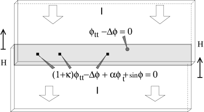
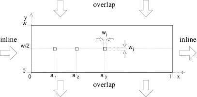
Fig. 1: The left panel shows the top view of a superconducting microstrip line containing three Josephson junctions. The parameters $H,I$ and $\phi$ are respectively the applied magnetic field, the current and the phase difference between the two superconducting layers. The right panel shows the associated 2D domain of size $l\times w$ containing $n=3$ junctions placed at the positions $y=w/2$ and $x=a_{i},~{}i=1,n$.

where $C_{j}$ is the capacity of the junction per unit area, $R$ the resistance per unit area due to normal electrons. The branch inductance $L=\mu_{0}d_{0}$ involves the magnetic thickness $d_{0}$, a quantity used by experimentalists. In the microstrip $\Omega-\Omega_{j}$, the Josephson and quasi-particle currents are absent so one obtains the wave equation,

$$C_{l}\Phi_{tt}-\frac{1}{L_{l}}\Delta\Phi=0~{}~{},$$ (3)

where the $l$ subscripts indicate that we are in the linear region (i.e.: outside the junction). For inhomogeneous circuits like the one of Fig. 1 these two equations can be written as [15, 16]

$${C_{l}}\Phi_{tt}-\nabla\left({1\over L(x)}\nabla\Phi\right)+g(x,y)\left[(C_{j}-C_{l})\Phi_{tt}+J_{c}\sin\left({\Phi\over\Phi_{0}}\right)+{\Phi_{t}\over R}\right]=0,$$ (4)

where $g=1$ in the junctions and 0 outside. This formulation guarantees the continuity of the phase and its normal gradient across the interfaces. At this point we will assume the same surface inductance $L$ in the junctions and linear region. This simplifies greatly the formulation and can be realized in practical situations. To normalize the equation, we introduce the units of length and time, respectively the Josephson length $\lambda_{J}$ and plasma frequency $\omega_{p}$

$$\lambda_{J}=\sqrt{\frac{\Phi_{0}}{J_{c}L_{l}}}\;,~{}~{}~{}\frac{1}{\omega_{p}}=\sqrt{\frac{C_{l}\Phi_{0}}{J_{c}}}\;.$$ (5)

Finally we normalize space, time and phase as

$$\tilde{x}=x/\lambda_{J},~{}~{}\tilde{y}=y/\lambda_{J},~{}~{}\tilde{t}=t\omega_{p},~{}~{}\varphi=\Phi/\Phi_{0},$$ (6)

to get the normalized 2D inhomogeneous perturbed sine-Gordon equation

$$\varphi_{\tilde{t}\tilde{t}}-\Delta\varphi+g(\tilde{x},\tilde{y})(\kappa\varphi_{\tilde{t}\tilde{t}}+\alpha\varphi_{\tilde{t}}+\sin\varphi)=0$$ (7)

where the coefficients $\alpha$ and $\kappa$ are

$$\kappa=\frac{{C_{j}}}{{C_{l}}}-1,~{}~{}~{}\alpha=\frac{1}{{R}}\sqrt{\frac{\Phi_{0}}{J_{c}{C_{l}}}}\;.$$ (8)

The boundary conditions are

$$\varphi_{\tilde{x}}|_{({\tilde{x}}=0)}={\tilde{H}}+(1-\nu)\frac{\tilde{I}}{2\tilde{w}},~{}~{}~{}\varphi_{\tilde{x}}|_{({\tilde{x}}={\tilde{l}})}={\tilde{H}}-(1-\nu)\frac{\tilde{I}}{2\tilde{w}},$$ (9)

$$\varphi_{\tilde{y}}|_{({\tilde{y}}=0)}=\nu\frac{\tilde{I}}{2\tilde{l}},~{}~{}~{}\varphi_{\tilde{y}}|_{({\tilde{y}}={\tilde{w}})}=-\nu\frac{\tilde{I}}{2\tilde{l}},$$ (10)

where

$$\tilde{H}=H\frac{\lambda_{J}d_{0}}{\Phi_{0}}\;,~{}~{}\tilde{I}=I\frac{\mu_{0}d_{0}}{\Phi_{0}}=\frac{LI}{\Phi_{0}}\;,$$ (11)

and $l$ and $w$ are normalized by $\lambda_{J}$. After this section all tildes will be omitted for simplicity.

2.2 The $1D$ model

This equation is difficult to analyze and its solutions can only be obtained numerically. In addition most real devices have a width that is much smaller than their length and the junctions are distributed symmetrically so that it is reasonable to reduce the problem to one dimension. To do this we expand $\varphi$ on transverse Fourier modes

$$\varphi(x,y,t)=\frac{\nu\gamma}{2l}\left(y-\frac{w}{2}\right)^{2}+\sum^{\infty}_{n=0}\phi_{n}(x,t)\cos\left(\frac{n\pi y}{w}\right)\;,$$ (12)

where $\gamma=I/w$ and the first term takes care of the boundary condition (9). After inserting (12) into (7) and integrating across $y$ we get the evolution of $\phi_{0}$

$$\phi_{tt}-\phi_{xx}+{w_{j}\over w}g(x,y=0)(\kappa\phi_{tt}+\alpha\phi_{t}+\sin\phi)=\nu{\gamma\over l}\;,$$ (13)

where we omitted the $0$ in $\phi_{0}$ and terms in $\phi_{i},i\geq 1$ which are small because of the smallness of the current [17].

The boundary conditions are

$${\phi}_{x}|_{x=0}=H-(1-\nu){\gamma\over 2},~{}~{}~{}~{}{\phi}_{x}|_{x=l}=H+(1-\nu){\gamma\over 2},$$ (14)

and

$$g(x)=\left\{\begin{array}[]{l r}\frac{w_{j}}{w},&a_{j}-\frac{l_{j}}{2}<x<a_{j}+\frac{l_{j}}{2},\\ 0,&{\rm elsewhere}.\\ \end{array}\right..$$

The factor $w_{j}/w$ is exactly the ”rescaling” of $\lambda_{J}(=1)$ into $\lambda_{eff}=\sqrt{w\over w_{j}}>1$ due to the presence of the lateral passive region [18].

As the area of the junction is reduced the total super-current is reduced and tends to zero. Small junctions where the phase variation can be neglected and that have a significant supercurrent we introduce the following Dirac distribution model. First define the function $g_{h}(x)$,

$$g_{h}(x)=\left\{\begin{array}[]{l r}\frac{w_{j}}{wh},&a_{j}-\frac{hl_{j}}{2}<x<a_{j}+\frac{hl_{j}}{2},\\ 0,&{\rm elsewhere},\\ \end{array}\right.$$

notice that $g_{1}(x)=g(x)$. When the junction widths $w_{j}\ll\lambda_{J}$ we can further reduce the problem by neglecting the variation of the phase inside the junctions. We then obtain the Dirac delta function distributed model [15, 16] by making $h$ tend to $0$. For an $n$ junctions device,

$$\lim_{h\to 0}g_{h}(x)=\sum_{j=1}^{n}\frac{w_{j}l_{j}}{l}\delta(x-a_{j}).$$

Finally we obtain the $\delta-1D$ model for the device,

$${\phi}_{tt}-{\phi}_{xx}+\sum_{j=1}^{n}d_{j}\delta(x-a_{j})(\kappa{\phi}_{tt}+\sin{\phi}+\alpha{\phi}_{t})=\nu\frac{\gamma}{l},$$ (15)

where

$$d_{j}=\frac{w_{j}l_{j}}{w}$$ (16)

and where the boundary conditions are given by eq.(14). This is the main model of the article and we will analyze it in detail.

3 Preliminary analysis

From the Josephson equation (1) it can be seen that ${\phi}_{t}$ is a voltage. In experiments this instantaneous voltage is of very high frequency ($\sim$ 500 GHz) and can only be detected by making it beat with a well-known source. On the other hand the time average voltage can be measured in a fairly standard way. This current voltage relation (the $I-V$ curve) is a characterization of the device. It is therefore important for the analysis to explain it. We now give some important symmetries of the $I-V$ curve. The first one is the periodicity with respect to the magnetic field $H$. This is similar to the one obtained in the static case [9].

3.1 Periodicity of the $I-V$ curve with $H$

The $I-V$ curve of the device modeled by eq.(15) and (14) depends on the magnetic field $H$. We denote $I-V|_{H}$ the $I-V$ curve of the device for the magnetic field $H$. Let us introduce $l_{j}=a_{j+1}-a_{j}$ the distance between two consecutive junctions. Let $l_{min}$ be the smallest distance $l_{j}$. We define a harmonic array as a circuit where $l_{i}$ is a multiple of $l_{min}$ for all $i$.

Proposition, Periodicity of the device:

For a harmonic circuit, the $I-V|_{H}$ curve is periodic with a period $2\pi/l_{min}$.

Proof:

Let $\phi$ be a solution of (15) for a current $\gamma$ and a magnetic field $H$. We introduce $f(x)=(2\pi/l_{min})(x-a_{1})$ and $\psi(x;t)=\phi(x;t)+f(x)$. So $\psi$ verifies

$${\phi}_{tt}-{\phi}_{xx}+\sum_{j=1}^{n}\frac{w_{j}l_{j}}{l}\delta(x-a_{j})(\kappa{\phi}_{tt}+\sin({\psi}-f)+\alpha{\phi}_{t})=\nu\frac{\gamma}{l},$$ (17)

with $\psi_{x}(0;t)=H+2\pi/l_{i}-(1-\nu)\gamma/2$, and $\psi_{x}(l;t)=H+2\pi/l_{i}+(1-\nu)\gamma/2$. Since, $f(a_{j})=2k\pi$, $\forall i\in\{1;...;n\}$, then $\psi$ is a solution of (15) for $H+H_{p}\equiv H+2\pi/l_{min}$ and for the same $\gamma$.

Conversely, by subtracting $f$ from a solution associated to $H+H_{p}$ and a current $\gamma$, we obtain a solution for $H$ and the same current $\gamma$. We have shown that for a given $\gamma$ and $H$, if there is a solution, we can find another for $H+2k\pi/l_{min}$ ($k\in{Z}$). We obtain the same $I-V$ curves.

$$I-V|_{H+H_{p}}=I-V|_{H}.$$ (18)

with $H_{p}=2\pi/l_{min}$.

In the non harmonic case, if the junctions are set such that $l_{j}=p_{j}/q_{j}$, where $p_{j}$ and $q_{j}$ are integers, prime with each other, then $I-V|_{H}$ is periodic with period $H_{p}$ such that

$$H_{p}=2\pi\frac{LCM(q_{1};...;q_{n-1})}{HCF(p_{1};...;p_{n-1})},$$ (19)

where $LCM$ is the Lowest Common Multiple and $HCF$ the Highest Common Factor. To prove this write $f(x)=H_{p}(x-a_{1})$ and use again the previous argument.

3.2 The high voltage approximation

When the voltage $\phi_{t}$ is large, the phase $\phi$ is rotating fast so that one can write

$$\phi(x,t)=Vt+\psi(x,t),$$ (20)

where the average

$$\left<\psi\right>\equiv{1\over T}\int_{t}^{t+T}\psi(x,t^{\prime})dt^{\prime}\equiv\phi_{v}(x).$$ (21)

Plugging the ansatz (20) into (15) and taking the average we get

$$\left<\psi_{tt}\right>-{\phi_{v}}_{xx}+\sum_{j=1}^{n}d_{j}\delta(x-a_{j})$$

$$\left[\kappa\left<\psi_{tt}\right>+\left<\sin(Vt)\cos(\psi)\right>+\left<\cos(Vt)\sin(\psi)\right>+\alpha\left<\psi_{t}\right>+\alpha V\right] = \gamma.$$

Then if we neglect the nonlinear terms we obtain the static equation, we obtain a new equation such that $\left<\psi_{tt}\right>=\left<\psi_{t}\right>=0$ is a solution. Thus,

$$-{\phi_{v}}_{xx}+\alpha V\sum_{j=1}^{n}d_{j}\delta(x-a_{j})=\nu{\gamma\over l},$$ (23)

together with the boundary conditions

$${\phi_{v}}_{x}|_{x=0}=H-(1-\nu){\gamma\over 2},~{}~{}{\phi_{v}}_{x}|_{x=l}=H+(1-\nu){\gamma\over 2}.$$ (24)

By integrating the equation (23) one sees that this problem has a solution if

$$V={\gamma\over\alpha\sum_{j}d_{j}}.$$ (25)

Let us write this high voltage solution for a device with many junctions. At each junction $x=a_{j}$, the phase must be continuous. Integrating equation (23) over a neighborhood of $a_{j}$ and taking the limit of this neighborhood going to zero one gets the jump condition

$$-\left[{\phi_{v}}_{x}\right]_{a_{j}^{-}}^{a_{j}^{+}}+\alpha V{d_{j}\over l}=0.$$ (26)

Notice also that outside the junctions, the solution has to be of the form

$$\phi_{v}(x)=-\nu{\gamma\over 2l}x^{2}+c_{1}x+c_{2}.$$

It is then natural to build the solution by steps, using a sort of shooting method. To simplify the discussion, let us consider a device with two junctions placed respectively at the positions $a_{1}$, $a_{2}$. We write

$$\phi_{v}(x)=\left\{\begin{array}[]{ll}\phi_{0}(x),&~{}0\leq x\leq a_{1},\\ \phi_{1}(x),&~{}a_{1}\leq x\leq a_{2},\\ \phi_{2}(x),&~{}a_{2}\leq x\leq l.\end{array}\right.$$ (27)

At each junction $a_{j}$ we have $\phi_{j+1}(a_{j})=\phi_{j}(a_{j})$ and

$${\phi_{j+1}}_{x}(a_{j}^{+})-{\phi_{j}}_{x}(a_{j}^{-})+\alpha V{d_{j}\over l}=0.$$

It is then natural to write

$$\phi_{0}(x)=-\nu{\gamma\over 2l}x^{2}+\left[H-(1-\nu)\frac{\gamma}{2}\right]x+C.$$ (28)

From the relations at each junction, we infer that

$$\phi_{1}(x)=\phi_{0}(x)+\gamma{d_{1}\over d_{1}+d_{2}}(x-a_{1}),$$

(29)

$$\phi_{2}(x)=\phi_{1}(x)+\gamma{d_{2}\over d_{1}+d_{2}}(x-a_{2}).$$

It can be checked that the right boundary condition for $x=l$ can verified by this formulation whatever the value of $H$ by choosing $\gamma$ thanks to eq.(25). The function $\phi_{v}(x)$ defined by the equations (28-29) is then the solution of the problem (23,24).

3.3 Simplification of the $\delta-1D$ model

The static part $\phi_{v}$ of the high voltage solution can be used to simplify the formulation of the problem, in particular the boundary conditions. For that we introduce

$$\psi(x,t)=\phi(x,t)-\phi_{v}(x),$$ (30)

so that the sine-Gordon equation (15) becomes

$$\psi_{tt}-\psi_{xx}+\sum_{j=1}^{n}d_{j}\delta(x-a_{j})\left[\kappa\psi_{tt}+\alpha\psi_{t}+\sin(\psi+\phi_{v})-\frac{\gamma}{\sum_{k=1}^{n}d_{k}}\right]=0\;,$$ (31)

with the homogeneous Neumann boundary conditions

$$\psi_{x}|_{x=0}=0,~{}~{}\psi_{x}|_{x=l}=0.$$ (32)

Equation (31) now contains for each junction a sine term with an argument that is shifted by $\phi_{v}(a_{j})-\phi_{v}(a_{1})$. When averaging over time we get

$$\left<\phi(a_{j})-\phi(a_{1})\right>_{t}\approx\phi_{v}(a_{j})-\phi_{v}(a_{1})\;.$$

We define $\Psi_{j}$ as the phase-shift of the junction $j$

$$\Psi_{j}=\phi_{v}(a_{j})-\phi_{v}(a_{1})\;.$$ (33)

By a simple translation, equation (31) becomes

$$\psi_{tt}-\psi_{xx}+\sum_{j=1}^{n}d_{j}\delta(x-a_{j})\left[\kappa\psi_{tt}+\alpha\psi_{t}+\sin(\psi+\Psi_{j})-\frac{\gamma}{\sum_{k=1}^{n}d_{k}}\right]=0\;.$$ (34)

The boundary conditions (32) are unchanged and $\Psi_{1}=0$.

4 Resonances for an array of point junctions

4.1 Spectral problem

When the system is on a resonance, the solution is periodic so that it can be written as $\psi(x,t)=e^{i\omega t}\varphi(x)$. In that case the terms $\alpha\psi_{t}+\gamma/\sum_{k=1}^{n}d_{k}$ globally balance each other. The sine term can be averaged out. Therefore to satisfy the equation (34) it is necessary that

$$\psi_{tt}-\psi_{xx}+\sum_{j=1}^{n}d_{j}\delta(x-a_{j})\kappa\psi_{tt}=0\;,$$ (35)

together with the homogeneous Neumann boundary conditions (32).

When the capacities per unit area of the junctions and passive regions are equal $\kappa=0$, so the array resonates on a cosine Fourier mode, see [15, 19].

$$\psi_{n}(x,t)=e^{i{n\pi t\over l}}\cos\left({n\pi x\over l}\right).$$

In this description, we have neglected the higher harmonics which decay exponentially as shown by numerical calculations. When $\kappa\neq 0$, the eigenmodes of equation (35) differ from $n\pi/l$. To analyze them we substitute $\psi(x,t)=e^{i\omega t}\varphi(x)$ into (35) and obtain the following eigenvalue problem

$$\varphi_{xx}+\omega^{2}\left[1+\sum_{j=1}^{n}d_{j}\delta(x-a_{j})\kappa\right]\varphi=0,$$ (36)

together with homogeneous Neumann boundary conditions for $\varphi$.

We consider the two junctions case. We will obtain results that can be generalized to an array with $n>2$ junctions. We introduce for ease of notation $\kappa_{j}=\kappa d_{j}$. It is then natural to assume a solution

$$\varphi(x)=\left\{\begin{array}[]{lll}A_{1}\cos(\omega x),&{\rm for}&0\leq x\leq a_{1},\\ A_{2}\cos(\omega x)+B_{2}\sin(\omega x),&{\rm for}&a_{1}\leq x\leq a_{2},\\ A_{3}\cos(\omega x)+B_{3}\sin(\omega x),&{\rm for}&a_{2}\leq x\leq l,\end{array}\right.$$ (37)

where the form of $\varphi$ in the first interval was chosen to satisfy the boundary condition at $x=0$. As usual $\varphi$ is continuous at the junctions $x=a_{j}$ and one can see that the jump of the derivative is

$$[\varphi_{x}]_{a_{j}^{-}}^{a_{j}^{+}}+\kappa_{j}\omega^{2}\varphi(a_{j})=0.$$ (38)

Writing these $2n=4$ conditions at the junctions and the boundary condition at $x=l$, one obtains a 5th order homogeneous system in $A_{1},A_{2},B_{2},A_{3},B_{3}$. The solution is non trivial if the following determinant is zero

$$\left\|\begin{array}[]{lcccr}C_{1}&-C_{1}&-S_{1}&0&0\\ S_{1}&-S_{1}+\kappa_{1}\omega C_{1}&C_{1}+\kappa_{1}\omega S_{1}&0&0\\ 0&C_{2}&S_{2}&-C_{2}&-S_{2}\\ 0&S_{2}&-C_{2}&-S_{2}+\kappa_{2}\omega C_{2}&C_{2}+\kappa_{2}\omega S_{2}\\ 0&0&0&-S_{l}&C_{l}\end{array}\right\|=0,$$ (39)

where $C_{1}=\cos(\omega a_{1}),~{}S_{1}=\sin(\omega a_{1}),~{}C_{2}=\cos(\omega a_{2}),~{}S_{2}=\sin(\omega a_{2}),~{}C_{l}=\cos(\omega l),~{}S_{l}=\sin(\omega l).$ When more junctions are present in the device, the determinant giving the dispersion relation can be generated by adding the elementary component in rows 3 and 4 corresponding to each additional junction.

We now give the resonant frequencies when there is only one junction. The determinant (39) becomes

$$\left\|\begin{array}[]{lcr}C_{1}&-C_{1}&-S_{1}\\ S_{1}&-S_{1}+\kappa_{1}\omega C_{1}&C_{1}+\kappa_{1}\omega S_{1}\\ 0&-S_{l}&C_{l}\end{array}\right\|=0,$$ (40)

which implies

$$\sin(\omega l)+\kappa\omega d_{1}\cos(\omega a_{1})\cos(\omega(l-a_{1}))=0.$$ (41)

Several remarks should be made on this relation.

• First, when $\kappa\ll 1$ we recover the usual $\sin(\omega l)=0$ dispersion leading to harmonic frequencies.

• The opposite limit $\kappa\gg 1$ is more interesting because it leads to a splitting of the oscillations in the left and in the right side of the film. We obtain $\cos(\omega a_{1})=0$ or $\cos(\omega(l-a_{1}))=0$ leading to $\omega a_{1}=(2n+1)\pi/2$ or $\omega(l-a_{1})=(2m+1)\pi/2$ where $m,n$ are integers.

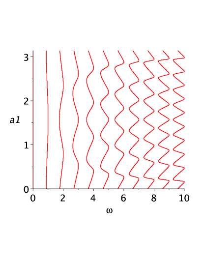
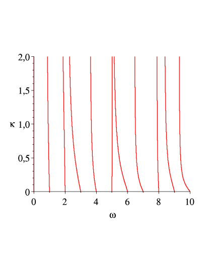
Fig. 2: Dependence of the eigenvalues (zeros of the dispersion relation (41) ) on the position of the junction $a_{1}$ in the microstrip (left panel) and on the capacity miss-match $\kappa$ (right panel). For the left panel, $\kappa=0.5$. For the right panel $a_{1}=0.3l=0.3\pi$.

Notice that Larsen et al [20] considered a centered junction $a_{1}=l/2$ in a microstrip. Their dispersion relation

$$\tan\pi{f\over f_{e}}=-\pi{C_{j}\over C_{e}}{f\over f_{e}},$$

is similar to the one we get with our approach except that the coefficient is different. We obtain using (41)

$$\tan(\omega l)=-\omega l\left({C_{j}\over C_{l}}-1\right){w_{j}^{2}\over wl}.$$ (42)

This latter expression gives the correct eigenmodes as shown in the current voltage characteristics computed numerically shown in the next sections.

4.2 Eigenvectors and inner product

We introduce here the inner product associated with the dispersion relation (41). The eigenvectors $\varphi_{i}$ (respectively $\varphi_{j}$) associated to the eigenvalue $\omega_{i}$ (resp. $\omega_{j}$) satisfy

$${\varphi_{i}}_{xx}+\omega_{i}^{2}\varphi_{i}\left(1+\delta(x-a_{1})\kappa_{1}\right) = 0,$$ (43)

$${\varphi_{j}}_{xx}+\omega_{j}^{2}\varphi_{j}\left(1+\delta(x-a_{1})\kappa_{1}\right) = 0,$$ (44)

together with the boundary conditions

$$\left.{\varphi_{i}}_{x}\right|_{x\in\{0,l\}}=0,~{}{\rm and}~{}~{}\left.{\varphi_{j}}_{x}\right|_{x\in\{0,l\}}=0.$$ (45)

We assume the eigenvalues to be different. As usual we multiply eq.(43) by $\varphi_{j}$ and eq.(44) by $\varphi_{i}$, substract the second from the first and integrate on the domain. We obtain

$$\int_{0}^{l}({\varphi_{i}}_{xx}\varphi_{j}-{\varphi_{j}}_{xx}\varphi_{i})dx+(\omega_{i}^{2}-\omega_{j}^{2})\left[\int_{0}^{l}\varphi_{i}\varphi_{j}dx+\kappa_{1}\varphi_{i}(a_{1})\varphi_{j}(a_{1})\right]=0.$$ (46)

The first integral is zero because of the boundary conditions (45). Since $\omega_{i}\neq\omega_{j}$ we get

$$\int_{0}^{l}(1+\kappa_{1}\delta(x-a_{1}))\varphi_{i}\varphi_{j}dx=0.$$ (47)

Thus we obtain the orthogonality of the eigenvectors $\varphi_{i}$, $i$ is an integer with the associated inner product defined by

$$\left<f;g\right>\equiv\int_{0}^{l}\left(1+\kappa_{1}\delta(x-a_{1})\right)fgdx.$$ (48)

It is then possible to normalize the eigenvectors so that they form an orthonormal basis. When there are $n$ junctions in the array, the inner product can be generalized easily to

$$\left<f;g\right>\equiv\int_{0}^{l}\left(1+\sum_{i=1}^{n}\kappa_{i}\delta(x-a_{i})\right)fgdx.$$ (49)

In the case of a single junction, the normalized eigenvectors $\varphi_{n}(x)$ are given by

$$\varphi_{n}(x)=\left\{\begin{array}[]{lll}A_{n}\cos(\omega_{n}x),&{\rm for}&0\leq x\leq a_{1},\\ A_{n}{\cos(\omega_{n}a_{1})\over\cos(\omega_{n}(l-a_{1}))}\cos(\omega_{n}(l-x)),&{\rm for}&a_{1}\leq x\leq l,\end{array}\right.$$ (50)

where $\omega_{n}$ satisfies the dispersion relation (41) and

$$A_{n}=\frac{1}{\sqrt{{l\over 2}+{\sin 2\omega_{n}a_{1}\over 4\omega_{n}}+{\cos^{2}\omega_{n}a_{1}\over\cos^{2}\omega_{n}(l-a_{1})}{\sin 2\omega_{n}(l-a_{1})\over 4\omega_{n}}+\kappa_{1}\cos^{2}\omega_{n}a_{1}}}.$$ (51)

Fig. 3 shows the 4 non trivial eigenmodes $\phi_{i},~{}i=1-4$ for a large capacity miss-match. Notice how the modes are almost zero on one side of the cavity.

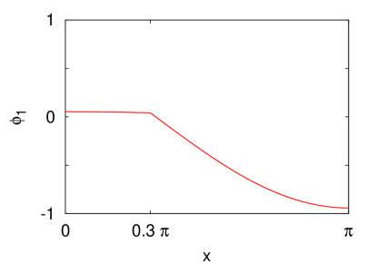
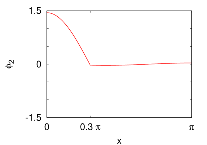
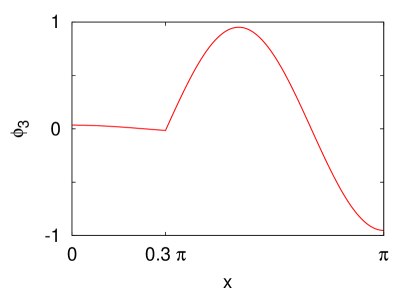
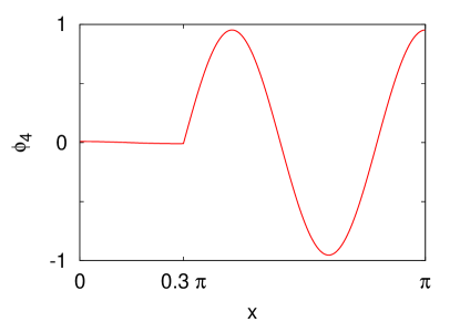
Fig. 3: Normalized eigenmodes $\varphi_{i}(x),i=1,2$ (top panels from left to right) and $\phi_{i}(x),i=3,4$ (top panels from left to right) for a large capacity miss-match $\kappa=30$. The other parameters are $d_{1}=1$, $l=\pi$ and $a_{1}=0.3\pi$.

4.3 Eigenvalues and $I-V$ curves

The eigenvalues calculated in the previous section appear as resonances in the current-voltage characteristics of the device. We computed the $I-V$ curves from the numerical solution of equation (15). The singular partial differential equation is integrated over reference volumes and the time advance is done by an ordinary differential equation solver (see Appendix 6 for more details). The average voltage $V\equiv\left<\phi_{t}\right>$ is computed over a time interval $10/\alpha$ after waiting a time $100/\alpha$ for the solution to stabilize. When the system is locked on a resonance, it oscillates periodically on an eigenfrequency solution of the dispersion relation eq.(41). We will show that the numerical solution follows closely the corresponding eigenvector.

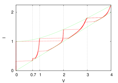
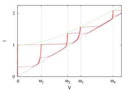
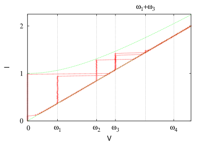
Fig. 4: $I-V$ curves for an array with one junction, $d_{1}=1$, $\alpha=0.5$, $l=\pi$, $a_{1}=0.3\pi$. Top panel, $\kappa=0$, middle panel $\kappa=1$ and bottom panel $\kappa=30$.

We choose a device with $l=\pi,~{}a_{1}=l/3,~{}d_{1}=1$ and take three limiting cases $\kappa=0$ $\kappa=1$ and $\kappa=30$. When there is no capacity miss-match ($\kappa=0$) we showed in [15] that the resonances of the $I-V$ curve are positioned at $V=k\pi/l$ with $k$ integer and are bounded by

$$\gamma l=d_{1}\alpha V,~{}{\rm and}~{}~{}\gamma l=d_{1}\sqrt{(\alpha V)^{2}+1}.$$

This is shown in the top panel of Fig. 4. In the middle panel we show the $I-V$ curve for $\kappa=1$. Notice how the resonances are not equally spaced and get sharper. The resonances are very close to the ones given by the dispersion relation, they are reported in table (1). Finally on the bottom panel we computed the $I-V$ curve for $\kappa=30$. This large value is typical in experiments where the oxide layer in the junction is about 100 times thinner than in the passive region. This together with the ratio $d_{1}=w_{j}^{2}/w$ gives $\kappa_{1}\approx 50$. Notice how the resonances are vertical indicating that the system is almost linear. This is to be expected because $\kappa\gg 1$ so that the sine term plays little role. The position of the resonances is exactly given by the dispersion relation (41). They are reported in the table (2) together with the coupling coefficient $\phi_{n}(a_{1})$. The eigenvalues are clearly not harmonic. Notice how some resonances do not go all the way to the junction curve. Another observation is that we have a resonance for $\omega_{2}$ even though the coupling coefficient is almost zero. We will come back to this point in the next section. Also it is interesting that there is no resonance for $\omega_{4}$.

$$\begin{array}[]{|c|c|c|c|}\hline\cr i&\omega_{i}&\cos(\omega_{i}a)&{\rm Normalization}~{}A_{i}\\ \hline\cr 0&0.&1.&0.491\\ \hline\cr 1&0.917&0.649&0.562\\ \hline\cr 2&1.931&-0.247&1.094\\ \hline\cr 3&2.438&-0.665&0.704\\ \hline\cr 4&3.682&-0.946&0.237\\ \hline\cr\end{array}$$

Table 1: Eigenvalues for the array of Fig. 4 with $\kappa=1$ (middle panel of Fig. 4).

$$\begin{array}[]{|c|c|c|c|}\hline\cr i&\omega_{i}&\cos(\omega_{i}a)&{\rm Normalization}~{}A_{i}\\ \hline\cr 0&0.&1.&0.1737\\ \hline\cr 1&0.734&0.770&5.341~{}10^{-2}\\ \hline\cr 2&1.687&-1.950~{}10^{-2}&1.447\\ \hline\cr 3&2.150&-0.440&3.462~{}10^{-2}\\ \hline\cr 4&3.575&-0.974&9.102~{}10^{-3}\\ \hline\cr\end{array}$$

Table 2: Eigenvalues for the array of Fig. 4 with $\kappa=30$ (bottom panel of Fig. 4).

Fig. 5 shows the eigenvectors in dashed line (green online) for a realistic value $\kappa_{1}=30$ corresponding to a capacity miss-match $\kappa=30$ and a surface ratio $d_{1}=w_{1}~{}l_{1}/w=1$. On the same plot are indicated in continuous line (red online) the instantaneous voltages $\varphi_{t}$ for different successive times. From top to bottom panels we show respectively the first, second and third resonance. One can see that the voltages follows very well the eigenvectors.

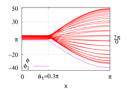
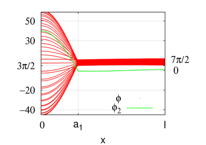
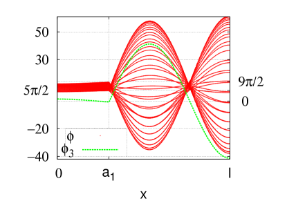
Fig. 5: Plot of the instantaneous voltage $\phi_{t}(x)$ for successive times for the first, second and third resonances in the $I-V$ curve for an array with one junction and with a large capacity miss-match $\kappa_{1}=30$. The corresponding eigenmodes (50) are plotted in dashed lines.

4.4 Projection on the normal modes

The normal modes that we have exhibited can be used to project the solution. This enables to analyze the dynamical behavior in a simple way. The eigenvectors solutions of the problem (43) are orthonormal for the inner product defined above. We will assume that all solutions $\phi$ belong to the vector space generated by the eigenvectors $\varphi_{i}$. This is difficult to justify theoretically but we will come back to this using the numerical results in the last section. Then the solution $\psi$ of equation (31) $\phi$ can be written as

$$\psi(x;t)=\sum_{i=0}^{+\infty}\beta_{i}(t)\varphi_{i}(x).$$ (52)

We assume the uniform convergence of the series (52) so that we can permute integrals and sums.

We will present the calculations for a single junction for simplicity. The results can be generalized to arrays with multiple junctions. We replace $\psi$ in eq.(31) for one junction,

$$\sum_{i=1}^{+\infty}\left(\beta_{i}^{\prime\prime}\varphi_{i}-\beta_{i}\varphi_{i}^{\prime\prime}\right)+$$

$$d_{1}\delta(x-a_{1})\left(\sum_{i=1}^{+\infty}\left(\kappa\beta_{i}^{\prime\prime}\varphi_{i}+\alpha\beta_{i}^{\prime}\varphi_{i}\right)+\sin\left(\psi+\Psi_{1}\right)-\frac{\gamma}{d_{1}}\right) = 0,$$

We multiply eq.(LABEL:dlt1D_vct) by $\varphi_{j}(x)$ and integrate it on its domain

$$\sum_{i=1}^{+\infty}\beta_{i}^{\prime\prime}\underbrace{\left(\int_{0}^{l}\varphi_{i}\varphi_{j}dx+\kappa_{1}\varphi_{i}(a_{1})\varphi_{j}(a_{1})\right)}_{=0~{}{\rm if}~{}i\neq j,~{}=1~{}{\rm else}}-\beta_{i}\int_{0}^{l}\varphi_{i}^{\prime\prime}\varphi_{j}dx+d_{1}\alpha\beta_{i}^{\prime}\varphi_{i}(a_{1})\varphi_{j}(a_{1})$$

$$+d_{1}\sin\left(\psi(a_{1})+\Psi_{1}\right)\varphi_{j}(a_{1})-\gamma\varphi_{j}(a_{1})=0.$$ (54)

and from eq.(36) we know that,

$$\varphi_{i}^{\prime\prime}=-\left(1+\kappa_{1}\delta(x-a_{1})\right)\omega_{i}^{2}\varphi_{i}.$$

Eq.(54) becomes

$$\beta_{j}^{\prime\prime}+\sum_{i=1}^{+\infty}\beta_{i}\omega_{i}^{2}\underbrace{\int_{0}^{l}(1+\kappa_{1}\delta(x-a_{1}))\varphi_{i}\varphi_{j}dx}_{=0~{}{\rm if}~{}i\neq j,~{}=1~{}{\rm else}}+\frac{d_{1}\alpha}{l}\beta_{i}^{\prime}\varphi_{i}(a_{1})\varphi_{j}(a_{1})$$

$$+\frac{d_{1}}{l}\sin\left(\psi(a_{1})+\Psi_{1}\right)\varphi_{j}(a_{1})-\gamma\varphi_{j}(a_{1})=0.$$ (55)

We obtain the final equation giving the evolution of $\beta_{j}$ in terms of $\phi$

$$\beta_{j}^{\prime\prime}+\omega_{j}^{2}\beta_{j}+c_{j}\left(\alpha\phi_{t}(a_{1})+\sin\left(\phi(a_{1})\right)-\frac{\gamma}{d_{1}}\right)=0,$$ (56)

where we have returned to the usual field $\phi$ and where the coupling coefficient $c_{j}$ is

$$c_{j}=d_{1}\varphi_{j}(a_{1}).$$ (57)

This coefficient does not depend directly on $\kappa$. Also notice that all equations are coupled by the same term

$$F\equiv\alpha\phi_{t}(a_{1})+\sin(\phi(a_{1}))-\frac{\gamma}{d_{1}},$$ (58)

where the coefficient $c_{j}$ regulates the forcing for each mode. When $n$ junctions are present in the device, the modal equations can be generalized to

$$\beta_{j}^{\prime\prime}+\omega_{j}^{2}\beta_{j}+\sum_{k=1}^{n}c_{j}^{k}\left(\alpha\phi_{t}(a_{k})+\sin\left(\phi(a_{k})\right)-\frac{\gamma}{\sum_{l=1}^{n}d_{l}}\right)=0,$$ (59)

where the generalized coupling coefficient $c_{j}^{k}$ is

$$c_{j}^{k}=d_{k}\varphi_{j}(a_{k}).$$ (60)

5 Numerical analysis of the IV curves

To analyze the mechanism leading to a resonance in the IV curves shown in Fig. 4 we project the numerical solution onto the normal modes that we defined in section 4. Following the definition of the inner product (48) we have

$$\beta_{i}=\left<\phi|\phi_{i}\right>\equiv\int_{0}^{l}\phi\phi_{i}dx+\kappa d_{1}\phi(a_{1})\phi_{i}(a_{1}).$$

The integral on the right hand side is computed using the trapeze method. Fig. 6 shows a plot of the amplitudes $\beta_{i},~{}i=1-4$ for the second resonance with $\kappa=1$ (middle panel for Fig. 4). Clearly $\beta_{2}$ is dominant. In the left panel we did not subtract the high voltage solution $\phi_{v}(x)$ (28-29) so that the other modes appear as parasites. If the high voltage solution is taken out then we have a clear dominance of $\beta_{2}$, all the other modes being close to 0. This shows that we have to a good approximation

$$\phi(x,t)\equiv\psi(x,t)+\phi_{v}(x)\approx\beta_{0}(t)\varphi_{0}(x)+\beta_{i}(t)\varphi_{i}(x)+\phi_{v}(x),$$ (61)

where $i=2$ and where we have included the 0 mode that is always present. We recover the results suggested by the plots of Fig. 5. We have observed this for all the resonances in the $I-V$ curve.

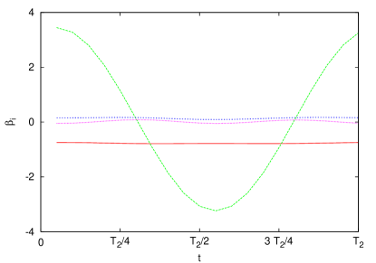
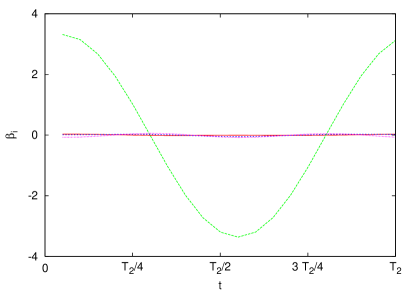
Fig. 6: Plot of the amplitudes $\beta_{i}(t),~{}i=1-4$ obtained by projecting the numerical solution for $\kappa=1$ at the top of the second resonance onto the normal mode $\varphi_{i}$. The modes are $\beta_{1}$ continuous line, (red online), $\beta_{2}$ dashed line (green online), $\beta_{3}$ short dash (blue online) and $\beta_{4}$ dotted line (pink online). In the left panel the projection is done directly on the solution $\phi(x,t)$. In the right panel we have subtracted the high voltage solution $\phi_{v}(x)$ for the given current $\gamma=1.36$. The time unit is the period $T_{2}=2\pi/\omega_{2}\approx 3.25$.

For example for $\kappa=30$ (bottom panel of Fig. 4) we show in Fig. 7 the amplitudes $\beta_{i}$ from top to bottom for the 1st , 2nd and 3rd resonance. Again the dominant amplitudes are from top to bottom $\beta_{1}$, $\beta_{2}$ and $\beta_{3}$.

Therefore the solution at the top of the resonances is given by (61) to a good approximation. To analyze how we reach this state we have projected the solution on the normal modes for increasing values of the current $\gamma$ all the way to the top of the resonance. The calculations were done over a long time interval (about 200 periods). Projecting the solution $\phi$ we observed a drift in the amplitudes $\beta_{i}$ due to the rapid increase of $\phi$ and the finite precision of the evaluation of the integrals. To avoid these technical problems we have projected the time derivative $\phi_{t}$. The qualitative conclusions are the same as for $\phi$ except that we will look at ${\beta_{i}}_{t}$. Fig. 7 shows three amplitudes as a function of time for $\gamma=1.12,~{}1.3,~{}1.42$ and $1.56$ and a voltage $V\approx\omega_{3}$ near the 3rd resonance for $\kappa=1$. Only three periods $T_{3}=2\pi/\omega_{3}$ have been represented for clarity, the rest of the time evolution is the same. In the top left panel for $\gamma=1.12$, the amplitude of the mode 3 is about 1 with small components in the modes 2 and 1. When the current is increased the amplitude of the 3rd mode increases and becomes periodic of period $T_{3}$. The other modes tend rapidly to 0.

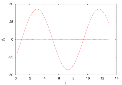
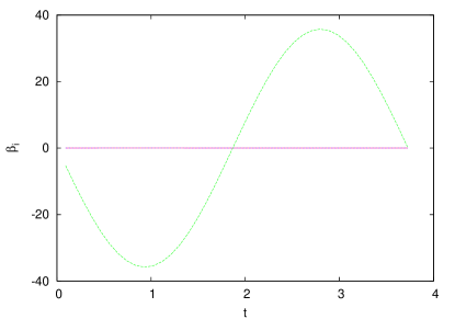
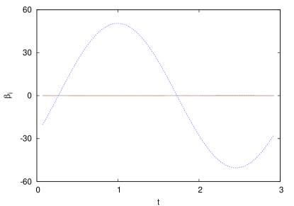
Fig. 7: Plot of the amplitudes $\beta_{i}(t),~{}i=1-3$ obtained by projecting the numerical solution at the top of the second resonance onto the normal mode $\varphi_{i}$ for $\kappa=30$. The dominant mode is resp. $i=1,2,3$ for resp. the 1st resonance (top panel), the second resonance (middle panel) and the third resonance (bottom panel).

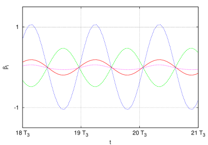
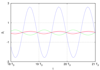
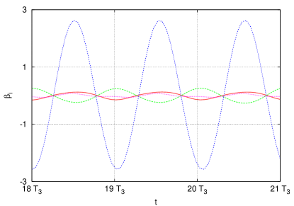
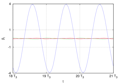
Fig. 8: Plot of the amplitudes of $\phi_{t}(x,t)$ as a function of time for four different values of the current, from top left to bottom right $\gamma=1.12,1.3,1.42,1.56$, on the third resonance $V=\omega_{3}$ for $\kappa=1$. The index of the modes are $i=1$ continuous (red online), $i=2$ dashed line (green online), $i=3$ short dash (blue online) and $i=4$ dotted line (pink online). The time interval is the period $T_{3}=2\pi/\omega_{3}\approx 2.58$.

It is instructive to compute numerically the forcing term $F$ as one progresses up the resonance. Fig. 9 shows $F(t)$ for three periods $T_{3}$ for the four values of $\gamma$ analyzed in Fig. 8. The amplitude of $F$ decreases for increasing $\gamma$ and $F$ becomes periodic of period $T_{3}$. This explains why we obtain the correct resonant modes using the spectral problem (36). Note that when $\kappa=0$ the forcing term $F$ of the amplitude equations tends to 0 when one gets close to the top of the resonances. Then one can solve the differential equation for $\phi(a_{1};t)$

$$\alpha\phi^{\prime}(a_{1};t)+\sin\left(\phi(a_{1};t)\right)-\frac{\gamma}{d_{1}}=0,$$ (62)

and close the system by expanding this solution using the standard Fourier modes[15]. This is not the case when $\kappa\neq 0$ as shown by these numerical results.

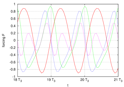
Fig. 9: Plot of the forcing term $F$ from (58) as a function of time for four different values of the current on the third resonance $V=\omega_{3}$ for $\kappa=1$. The values are $\gamma=1.12$ continuous (red online), $\gamma=1.3$ dashed line (green online), $\gamma=1.42$ short dash (blue online) and $\gamma=1.56$ dotted line (pink online). The time interval is the period $T_{3}=2\pi/\omega_{3}\approx 2.58$.

To analyze the resonances, we assume as in [12] that when in resonance, the solution has the spatial structure of the corresponding eigenmode.

$$\psi(x,t)=\beta_{0}(t)\varphi_{0}+\beta_{n}(t)\varphi_{n}(x),$$ (63)

where the first term on the right corresponds to the zero mode. The evolution of $\beta_{0},~{}\beta_{n}$ is then given by equation (56)

$$\beta_{n}^{\prime\prime}+\omega_{n}^{2}\beta_{n}+c_{n}F=0,$$ (64)

$$\beta_{0}^{\prime\prime}+c_{0}F=0,$$ (65)

where the forcing term is

$$F=\alpha\beta_{n}^{\prime}\varphi_{n}+\alpha\beta_{0}^{\prime}\varphi_{0}+\sin\left(\beta_{n}\varphi_{n}+\beta_{0}\varphi_{0}\right)-\frac{\gamma}{d_{1}}$$ (66)

To understand the specific shape of the resonances, the fact that we cannot obtain in the IV curve the right part of the resonance curve, one could carry out a bifurcation analysis similar to the one of [21]. However this is out of the scope of this article.

The situation is more complex when there are more junctions in the device. As an example we consider a two junction device with $l=\pi,~{}a_{1}=0.3\pi,~{}a_{2}=0.5\pi,~{}d_{1}=d_{2}=0.1$. The eigenmodes $\omega_{n}$ are plotted in Fig. 10 as a function of $\kappa$ and one can see them shift from integer values even for small $\kappa$.

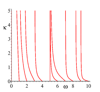
Fig. 10: Plot of the frequency $\omega$ vs. $\kappa_{i}$ for a device with two junctions where $a_{1}=0.3\pi,~{}a_{2}=0.5\pi,~{}d_{1}=d_{2}=0.1$.

In Fig. 11 we plot the $I-V$ curves obtained for this device for $\kappa=0,~{}4$ and 8 with $d_{1}=0.1$ so that $\kappa_{1}=d_{1}\kappa=0,~{}0.4$ and 0.8. The resonances observed correspond to the eigenfrequencies obtained. For $\kappa=0$ we have explained the height of the resonances using an approximate theory [19] based on the amplitude of oscillation of $\phi_{t}(a_{j})$ for each junction. This is the envelope function plotted in dashed line in the top left panel of Fig. 11. When $\kappa\geq 0$ it is more difficult. We think that this amplitude of oscillation, which can be obtain by the eigenvectors does not determine completely the height of the resonances.

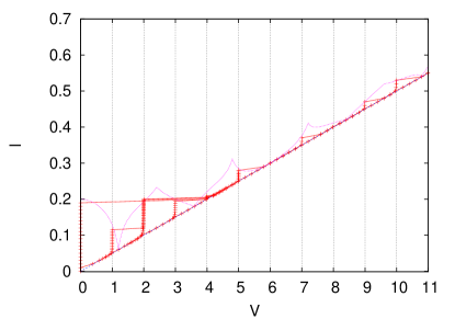
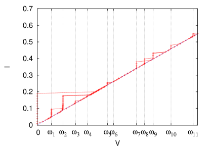
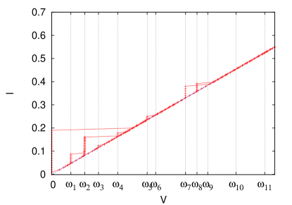
Fig. 11: IV curves for the two junction circuit studied in Fig. 10. The parameters are $l=\pi,d_{1}=d_{2}=0.1,~{}\alpha=0.25,~{}\kappa=0$. From top left to bottom $\kappa=0,4$ and 8. In the top panel the envelope function (see text) is plotted as a dashed line (pink online).

When the length of the device is larger more resonances can be accommodated in the $I-V$ curve. An interesting effect we found is that for large values of $\kappa$ the system locks to linear combinations of the eigenfrequencies. Such an example is shown in Fig. 12 for a two junction device in a microstrip of length $l=10$. For $\kappa\geq 5$ there appears in the $I-V$ curve a resonance for $\omega_{1}+\omega_{6}$. For $\kappa=10$ (bottom left panel) we see in addition resonances for $2\omega_{1},~{}\omega_{1}+\omega_{9}$. This is typical of a linear system. When we observe numerically the evolution of $\phi_{t}$ at this resonance we see the two eigenvectors 1 and 9. But we cannot explain this linear behavior: how the system can sum two non linear solution?

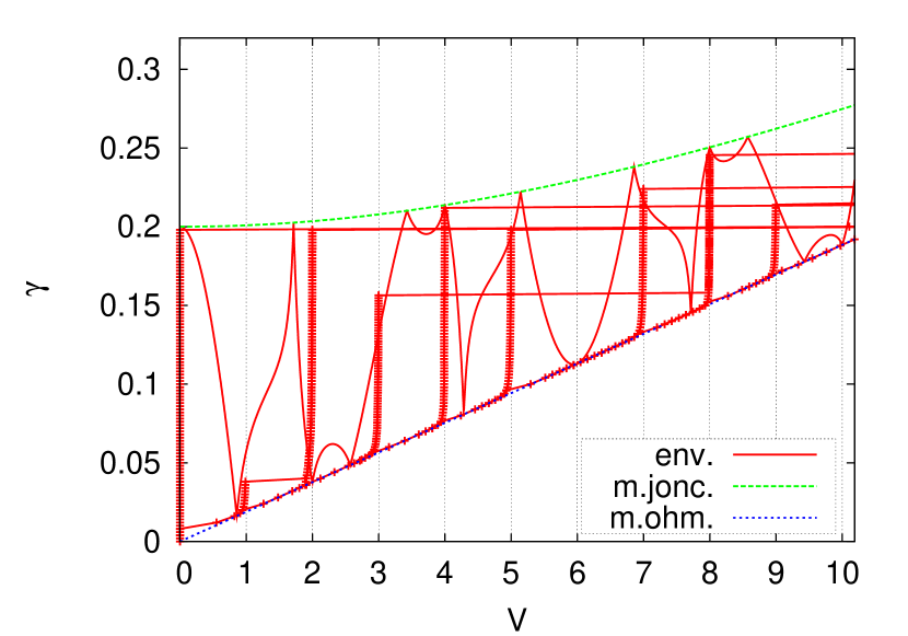
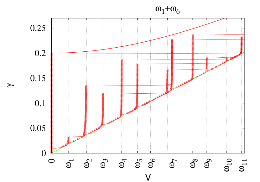
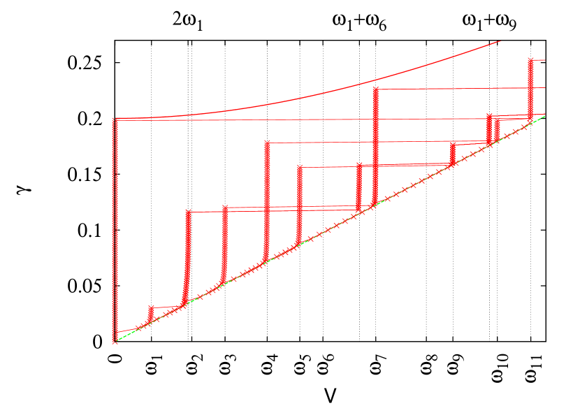
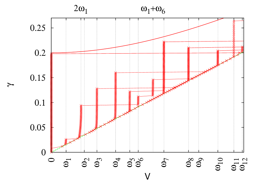
Fig. 12: $I-V$ curves of a two junction device, $a_{1}=10/3$, $a_{2}=25/3$, $l=10$, $d_{i}=0.1$, $\alpha=0.3$ and different values of $\kappa$. Top panels, $\kappa=0$ (left) and $\kappa=5$ (right). Bottom panels $\kappa=10$ (left) and $\kappa=22$ (right).

5.1 Conclusion

To summarize we have analyzed a long wave model describing a parallel array of Josephson junctions. We defined an appropriate spectral problem whose spectrum gives the resonances of any array with junctions of arbitrary (small) sizes and positions. This task would not have been possible without the complexity reduction provided by asymptotic analysis.

The adapted spectral problem leads to an inner product so that it becomes possible to project the dynamics of the system and describe arrays with more junctions.

It may now be possible to solve the inverse problem of finding the device yielding a given I-V curve. Another open question is the study of the amplitude equations (64) to analyze the stability of the resonances.

Acknowledgements

J.G.C. and L. L. thank Faouzi Boussaha and Morvan Salez for helpful discussions and for their experimental results. The computations were done at the Centre de Ressources Informatiques de Haute-Normandie (CRIHAN).

6 Appendix

The basis of the method is to discretize the spatial part of the operator and keep the temporal part as such. We thereby transform the partial differential equation into a system of ordinary differential equations. This method allows to increase the precision of the approximation in time and space independently and easily. In our case the operator is a distribution so that the natural way to give it meaning is to integrate it over a volume. We therefore choose as space discretisation the finite volume approximation where the operator is integrated over reference volumes. The value of the function is assumed constant in each volume. As solver for the system of differential equations, we use the Runge-Kutta method of order 4-5 introduced by Dormand and Prince implemented as the Fortran code DOPRI5 by Hairer and Norsett [22] which enables to control the local error by varying the time-step.

We first transform (..) into a system of first order partial differential equations We write $\psi(x,t)=\phi_{t}(x,t)$.

$$\left\{\begin{array}[]{r c l}\psi(x,t)&=&\phi_{t}(x,t)\\ \psi_{t}(x,t)&=&\phi_{xx}(x,t)-\delta(x-a)(\kappa\psi_{t}(x,t)+\alpha\psi(x,t))+d_{1}\sin(\phi(x,t)))+\nu\gamma/l\end{array}\right.$$ (67)

with the boundary conditions : $\phi_{x}|_{l\over 2}=H-(1-\nu)\gamma/2$, and $\phi_{x}|_{-{l\over 2}}=H+(1-\nu)\gamma/2$.

For simplicity we will describe the implementation of the finite volume discretisation in the case of a single junction. We introduce reference volumes $V_{k}$ whose centers we call $x_{k}$, $1\leq k\leq nn$. The discretisation points are placed such that the point $x_{ng+1}$ is at the junction, ($x_{ng+1}=a$). We thus define $x_{k}$ and $V_{k}$ using the following identities

$$V_{k}=\left]x_{k}-{h_{g}\over 2},x_{k}+{h_{g}\over 2}\right[~{},~{}~{}0<k<ng+1$$

with $(ng+1)h_{g}=a$

$$V_{k}=\left]x_{k}-{h_{d}\over 2},x_{k}+{h_{d}\over 2}\right[~{},~{}~{}ng+1<k<nn+1$$

with $(nn-ng)h_{d}=l-a$. Finally at the junction, $k=ng+1$

$$V_{k_{ng+1}}=\left]x_{ng+1}-{h_{g}\over 2},x_{ng+1}+{h_{d}\over 2}\right[.$$

$nn$, $ng$ and $nd$ are respectively the total number of discretisation points, the number of points to the left of the junction and the number of points to the right.

For a fixed t, we assume $\phi(x,t)$ to be constant on each volume $V_{k}$, so that

$$\int_{x_{k}-{h\over 2}}^{x_{k}+{h\over 2}}\phi(x,t)dx=h\phi(x_{k},t)~{}{\rm,~{}~{}with}~{}h=hg~{}{\rm or}~{}h=hd$$

Integrating over $V_{k}$ yields:

In the linear part of the partial differential equation : $0<k<nn+1$ and $k\neq ng+1$:

$$\left\{\begin{array}[]{r c l}\psi(x_{k},t)&=&\phi_{t}(x_{k},t)\\ \psi_{t}(x_{k},t)&=&\frac{\phi(x_{k+1},t)-2\phi(x_{k},t)+\phi(x_{k-1},t)}{h^{2}}+j\end{array}\right.$$ (68)

with $h=hg$ for $0<k<ng+1$ or $h=hd$ for $k>ng+1$. We recognize the usual discretisation of the second derivative.

At the junction: $k=ng+1$, we obtain

$$\int_{x_{ng+1}-{h_{g}\over 2}}^{x_{ng+1}+{h_{d}\over 2}}\delta(x-a)\left(\kappa\phi_{tt}(x,t)+\alpha\phi_{t}(x,t)+d_{1}\sin(\phi(x,t))\right)=$$

$$d_{1}\sin(\phi(x_{ng+1},t))+\alpha\phi_{t}(x_{ng+1},t)$$

So that the final system is:

$$\psi(x_{ng+1},t) = \phi_{t}(x_{ng+1},t)$$

$$\psi_{t}(x_{ng+1},t) = \left[\frac{4}{hg+hd}\left(\frac{\phi(x_{ng+2},t)-\phi(x_{ng+1},t)}{hg/2}-\frac{\phi(x_{ng+1},t)-\phi(x_{ng},t)}{hd/2}\right)\right.$$

$$\left.-\frac{2}{hg+hd}\left(d_{1}\sin(\phi(x_{ng+1},t))+\alpha\phi_{t}(x_{ng+1},t)\right)+j\right]\frac{1}{1-d_{k}\kappa}$$

The previous system of ordinary differential equations is then integrated numerically using the DOPRI5 integrator.

References

- [1] B. D. Josephson, Phys. Lett. 1, 251, (1962).
- [2] A. Barone and G. Paterno, Physics and Applications of the Josephson effect, J. Wiley, (1982).
- [3] K. Likharev, Dynamics of Josephson junctions and circuits, Gordon and Breach, (1986).
- [4] M. Salez et al., Proc. SPIE Conf. on Telescopes and Astronomical Instrumentation, Hawaii, 2002 (August 22-28), col. 4855, p. 402, Proc. 4th European Conference on applied superconductivity, EUCAS 99, 651, (1999)
- [5] F. Boussaha et al., Fundamental and harmonic submillimeter-wave emission from parallel Josephson junction arrays, J. of Applied Physics 105, 073902, (2009).
- [6] B. Vasilic, P. Barbara, S. V. shitov and C. J. Lobb Phys. Rev. B, 65, 180503(R), (2002).
- [7] J. G. Caputo, N. Flytzanis and M. Vavalis, A semi-linear elliptic pde model for the static solution of Josephson junctions, International Journal of Modern Physics C, vol. 6, No. 2, 241-262, (1995).
- [8] J. G. Caputo, N. Flytzanis, A. Tersenov and M. Vavalis, Analysis of a semi-linear pde for modeling static solutions of Josephson junctions, SIAM J. of Math. Analysis, 34, 1356-1379, (2003).
- [9] J. G Caputo and L. Loukitch, Statics of point Josephson junctions in a micro strip line, SIAM J. Appl Math, 67, No. 3, 810-836, (2007).
- [10] M. Salez, F. Boussaha, L. Loukitch and J. G. Caputo, Interference filter properties of nonuniform Josephson junction arrays, J. Appl. Phys. 102, 083904, (2007).
- [11] J. G. Caputo and L. Loukitch, Designing arrays of Josephson junctions for specific static responses, Inverse Problems 24 No 2 (April 2008), 025022.
- [12] I. O. Kulik, Soviet Physics-Technical physics, vol. 12, 1, 111-116, (1967).
- [13] M. Cirillo, N. Gronbech-Jensen, M. R. Samuelsen, M. Salerno and G. Verona Rinati, Fiske modes and Eck steps in long Josephson junctions: theory and experiments, Phys. Rev. B, 58, 12377, (1998).
- [14] J. Pfeiffer, A. A. Abdumalikov Jr., M. Schuster and A. V. Ustinov, Resonances between fluxons and plasma waves in underdamped Josephson transmission lines of stripline geometry, Phys. Rev. B, 77, 024511, (2008).
- [15] J. G. Caputo and L. Loukitch, Dynamics of point Josephson junctions in microstrip line., Physica 425 (2005) 69-89.
- [16] L. Loukitch, Modélisation et analyse mathématique d’un système à non-linéarites distribuées: les réseaux hétérogènes de jonctions Josephson, PhD thesis, INSA de Rouen, December 2006.
- [17] A. Benabdallah, J. G. Caputo and N. Flytzanis, Physica D 161, 79-101, (2002)
- [18] J. G. Caputo, N. Flytzanis and M. Vavalis, Effect of geometry on fluxon width in a Josephson junction, Journal of Modern Physics C, vol. 7, No. 2, 191-216, (1996).
- [19] J. G. Caputo and L. Loukitch, A system with distributed nonlinearities: the array of Josephson junctions, ”Nonlinear waves in complex systems: energy flow and geometry”, Collection ”Special Topics” of European J. Phys. 147, (1), (2007).
- [20] A. Larsen, H. Dalsgaard Jensen, J. Mygind, Phys. Rev. B, vol. 43, 10179-10190, (1991).
- [21] D. L. Brown, M. G. Forest, B. J. Miller and N. A. Petersson, Computation and stability of fluxons in a singularly perturbed sine-Gordon model of the Josephson junction, Siam J. Appl. Math, 54, 1048-1066, (1994).
- [22] E. Hairer, S. P. Norsett and G. Wanner. Solving ordinary differential equations I, Springer-Verlag, (1987).