Log-periodic oscillations for diffusion on self-similar finitely ramified structures

Abstract

Under certain circumstances, the time behavior of a random walk is modulated by logarithmic periodic oscillations. The goal of this paper is to present a simple and pedagogical explanation of the origin of this modulation for diffusion on a substrate with two properties: self-similarity and finite ramification order. On these media, the time dependence of the mean-square displacement shows log-periodic modulations around a leading power law, which can be understood on the base of a hierarchical set of diffusion constants. Both the random walk exponent and the period of oscillations are analytically obtained for a pair of examples, one fractal, the other non-fractal, and confirmed by Monte Carlo simulations.

I Introduction

Diffusion on non-Euclidean media is not a new research area. For example, the underlying mechanisms of the sub-diffusive behavior, characteristic of fractals, were discovered some decades ago. Indeed, it is by now well established that, on these objects, the spreading of the probability density function is continuously retarded because of the presence of holes of all sizes (the interested reader can refer to ale ; ram ; ben ; hav ; bou , and references therein). However, in the last years, considerable effort has been dedicated to investigate an outstanding phenomenon. It has been repeatedly reported that, on some deterministic fractals or self-similar graphs, the time behavior of a random walk (RW) is modulated by logarithmic-periodic oscillations gra ; kro ; ace ; bab1 ; bab2 ; maltz . Similar effects were observed for biased diffusion of tracers on random systems bernas ; stau0 ; stau ; yu , and out of the domain of diffusive motion, examples have been detected in earthquakes huang ; saleur , escape probabilities in chaotic maps close to crisis pola , kinetic and dynamic processes on random quenched and fractal media kut ; andra ; bab3 ; saleur2 , diffusion-limited aggregates sor1i , growth models huang2 , and stock markets near a financial crash sor2 ; van1 ; van2 ; van3 . There is general agreement that these oscillations are a manifestation of an inherent self-similarity dou , responsible for a discrete scale invariance sor1 .

A wide class of systems exhibiting log-periodicity is that of self-similar finitely ramified structures. Indeed, several researchers have found that, on these substrates, the root-mean-square displacement (RMSD) of a single RW as a function of time, follows an anomalous power law modulated by logarithmic periodic oscillations bab1 ; bab2 ; maltz (for related behavior, see gra ; kro ; ace and dou ). In this paper, we revisit this problem, with the purpose of explaining the origin of the behavior described above in a simple and comprehensible way. The work is a natural continuation of a previous one lore1 , where we studied log-periodic modulation in one-dimensional RW.

Our approach is two-fold: theoretical analysis and numerical simulations. In the theoretical part, we treat the diffusion problem in a quite general way. The analysis is facilitated by the fact that a part of a finitely ramified object can be separated from the rest by cutting a finite number of connections, which, because of self-similarity, does not depend on the size of the part to remove. For pedagogical reasons, the procedure is illustrated by two simple examples but the method should be easily generalized for other finitely ramified substrates. The first model of substrate, denoted I, is the well-known Vicsek’s snowflake fractal structure vic . The second, Model II, is also finitely ramified but may be considered a trivial fractal (with a fractal dimension of $2$ and without holes of all sizes). Model I is an example of what we will call a perfect diffusive self-similar structure; Model II corresponds to what we will call an asymptotically diffusive self-similar one. For both models we predict a time-modulated oscillatory behavior, and calculate the RW exponent and the period of the oscillations. The goal of the numerical part is to get some independent confirmation of the derived properties. We study, using standard Monte Carlo (MC) simulations, the time evolution of a particle diffusing on each substrate, and compare the findings with our theoretical predictions.

The paper is organized as follows. In Sec. II we define the models, discuss the causes for modulated power-law behavior and derive the RW time evolution. The outcome of MC simulations are presented in Sec. III. Finally, we give our conclusions in Sec. IV.

II Analytic Approach

The above mentioned substrates are built in stages on a square lattice and the result of every stage is called a generation. The structure of each generation is a periodic array of basic or unit cells, which consist of sites connected by bonds. We denote by $L$ the linear size of the unit cell that corresponds to the first generation.

On any generation, the motion of a single particle, initially located at a symmetry point of the structure, occurs stochastically. The particle jumps, with a hopping rate $k$, only between NN substrate sites which are connected by a bond.

II.1 Model I

The building process is illustrated in Fig. 1. Parts (a), (b) and (c) of this figure show the unit cell for the zeroth, first and second generation, respectively. It is easy to see that, for this model, $L=3a$, where $a$ is the distance between nearest-neighbor (NN) sites ($a=1$ in the rest of the article).

Figure 1: The unit cells of Model I. The zeroth, first, and second generations are shown in (a), (b), and (c), respectively. $L$ (3 in this case) is the linear size of the first generation.

It is also apparent from this figure that the second-generation basic cell has a linear size $L^{2}$ and is built from the first-generation one in a self-similar way. In general, the $n$-th generation basic cell has a linear size $L^{n}$ and, for $n>1$, a central part of a linear size $L^{(n-m)}$ (with $m=1,2,...,n-1$) can be separated from the rest by cutting only four bonds.

For the $n$-th generation, a two-dimensional periodic substrate is built by connecting the corresponding basic cell (the first-generation substrate can be observed at the top of Fig. 2). The final full self-similar substrate, we are interested in, is obtained after an infinite number of iterations. Note that, in this limit, the unit cell is identical to the snowflake fractal.

We proceed now to analyze the behavior of the diffusing particle. It is useful to remember that, on any periodic substrate, normal diffusion should be observed if time is long enough for the RW to be influenced by the structure periodicity. Thus, for the $n$-th generation substrate, a diffusion coefficient $D^{(n)}$ can be defined through the time dependence of the mean-square displacement $\langle\Delta^{2}x\rangle(t)=\langle[x(t)-x(0)]^{2}\rangle$ in the $x$ direction,

$$\langle\Delta^{2}x\rangle(t)=2D^{(n)}t,$$ (1)

which holds for a time $t$ longer that the average time for the particle to escape from the initial unit cell. Because of the $x\leftrightarrow y$ symmetry, the same time dependence holds for the mean-square displacement in $y$ direction.

It is not hard to convince oneself that the zeroth-generation substrate is the simple square lattice (see Fig. 1-(a)), and then

$$D^{(0)}=k.$$ (2)

The first-generation substrate is shown at the top of Fig. 2. However, regarding $x$-direction diffusion, the whole substrate and the string of cells displayed at the bottom of Fig. 2, with periodic boundary conditions in the $y$-direction, lead to equivalent problems. We exploit this equivalence and calculate the diffusion coefficient of that one-dimensional array of equivalent cells. Following the steady-state method of Ref. celso , we obtain

$$D^{(1)}=(3/5)k.$$ (3)

The reduction to a quasi one-dimensional problem is possible for every $n$, and, after some simple algebra, it is found that

$$D^{(n)}=(3/5)^{n}k,\;\;\;\mbox{for}\;n=0,1,2,....$$ (4)

On the base of this result, we can anticipate that, on the full self-similar structure, a RW will show a log-periodic modulated behavior. The key point here is that the diffusion coefficients satisfy

$$D^{(n)}/D^{(n+1)}=\delta,\;\;\;\mbox{for}\;n=0,1,2,...,$$ (5)

with $\delta=5/3$.

Figure 2: First generation of Model I. Top: the substrate built with the basic cell shown in Fig. 1-(b). Bottom: the infinite one-dimensional string of cells used to compute the diffusion coefficient $D^{(1)}$ (see Fig.2 in Ref. celso ). The arrows indicate periodic boundary condition in the $y$ direction meaning that when, for example, the RW at site a (b) jumps upward (downward), it will arrive at site b (a).

Let us start noting that, since at a time $t$ the particle will be located in a region of linear size of the order of the RMSD $\sqrt{\langle\Delta^{2}x\rangle(t)}$, for a time such that $AL^{n}<\sqrt{\langle\Delta^{2}x\rangle(t)}<AL^{n+1}$ ($A$ is a constant of the order of one), it will be impossible for the RW to distinguish the full self-similar substrate from the $(n+1)$-th-generation one. Everything will thus happen as on the latter and one should expect that

$$\langle\Delta^{2}x\rangle(t)=2D^{(n)}t,$$ (6)

for $t$ in that interval.

At later times, when the RMSD is of the order of $L^{n+1}$, the particle will start to diffuse as if located on the $(n+1)$-th generation substrate. The relation

$$\langle\Delta^{2}x\rangle(t)=2D^{(n+1)}t$$ (7)

will thus hold for $AL^{n+1}<\sqrt{\langle\Delta^{2}x\rangle(t)}<AL^{n+2}$.

Because of the substrate full self-similarity, we should observe a sequence of length-dependent diffusion coefficients, giving rise to the qualitative behavior depicted in Fig. 3. This is a sketch of the mean-square displacement as a function of time (thick curve), which has a power law form modulated by a log-periodic amplitude. That is,

$$\centering\langle\Delta^{2}x\rangle(t)=Ct^{2\nu}f(t){\rm,}\@add@centering$$ (8)

where $\nu$ is the RW exponent, $f(t)$ is a log-periodic function which satisfies $f(t\tau)=f(t)$, with the logarithmic period $\log(\tau)$, and the constant $C$ is obtained by asking that the log-time average of $\log(f)$ over one period be zero (see, for more details, Fig. 5).

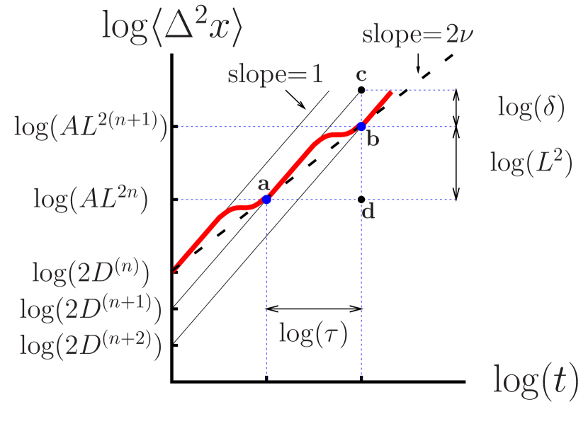
Figure 3: (Color online) Schematic of the mean-square displacement as a function of the time, shown by the thick red curve. The length of the segment bc is $\log(2D^{(n)})-\log(2D^{(n+1)})=\log(\delta)$, because of Eq. (5). From the slopes ($=1$) of the full straight lines (representing the normal diffusion behaviors, $\langle\Delta^{2}x\rangle=2D^{(n)}t$), one gets that the segments ad and cd have the same length or, equivalently, that $\log(\tau)=\log(L^{2})+\log(\delta)$. The dashed straight line represents the global power law $\langle\Delta^{2}x\rangle\sim t^{2\nu}$, with $2\nu=\log(L^{2})/\log(\tau)$. More details in the text.

In Fig. 3, two groups of inclined straight lines were drawn as a guide. The dashed line has a slope of $2\nu$ and corresponds to the $\langle\Delta^{2}x\rangle$ global power-law trend. The solid lines have slopes of $1$ and represent normal diffusion in each of the different generation structures. Both $\tau$ and $\nu$ can be expressed in terms of $L$ and $\delta$. It is clear from the slopes of the straight lines that $\log(\tau)=\log(L^{2})+\log(\delta)$ (solid line) and $2\nu=\log(L^{2})/\log(\tau)$ (dashed line), which is equivalent to

$$\tau=\delta L^{2}=L^{1/\nu}\;{\rm,}$$ (9)

and

$$\nu=\frac{1}{2+\frac{\log\delta}{\log L}}\;\;\;.$$ (10)

Note that, since $\delta>1$, anomalous sub-diffusion results ($\nu<1/2$, see Eq.10), and that, according to the sketch in Fig. 3, the amplitude of the modulation increases with the increase of $\delta$.

We would like to stress again that the self-similarity in the mean-square displacement, schematically shown in Fig. 3 and mathematically described by Eq.(8), is a direct consequence of (5). It is because of the latter that, in Fig. 3, the distance between any pair of nearest solid straight lines is a constant, and that two nearest equivalent points (like a and b) are always related by the transformation ($t\rightarrow\tau t$ , $\langle\Delta^{2}x\rangle\rightarrow\tau^{2v}\langle\Delta^{2}x\rangle$). The set of equations (5) also allows us to obtain analytically both the random walk exponent and the period of the oscillations. We will refer to Model I as a perfect diffusive self-similar structure. Other examples of this kind of structures are the fractals shown in Fig.(1) of Ref. maltz .

II.2 Model II

For this model, the basic cells for the zeroth, first and second generation are shown in Fig. 4. The full self-similar substrate is obtained when the generation order $n$ goes to infinity. As for Model I, the width of the $n$-th-generation unit cell is $L^{n}$ (where $L=3$ is the width of the first-generation one), and, for $n>1$, a central part of linear size $L^{n-m}$ (for $m<n$) can be separated from the rest by cutting only four bonds. Again, this allows us to reformulate the RW problem on a one-dimensional array (similar to that shown in Fig. 2-bottom), and to compute the diffusion coefficients following the steady-state method celso .

Figure 4: The unit cells of Model II. The zeroth, first, and second generations are shown in (a), (b), and (c), respectively. $L=3$, as in Model I. The dashed lines correspond to the bonds which are removed from the immediately previous generation. Note that, for every order, two NN unit cells are connected by only one bond.

It is evident that $D^{(0)}$ is given by Eq. (2). For the next two generations we obtain

$$D^{(1)}=(1/2)k,$$ (11)

and

$$D^{(2)}=(45/174)k.$$ (12)

We stop here because the calculations become more tedious for higher orders. However, at this point, we are already able to grasp the general trend, and to make a comparison between the two models.

From the values of the first few diffusion coefficients (Eqs. (2), (11) and (12)), we immediately observe that the ratio $D^{(0)}/D^{(1)}=2$ is different than $D^{(1)}/D^{(2)}=87/45\simeq 1.933$. In general, an analysis of the structures indicates that, for Model II, the equations (5) should be replaced by

$$D^{(n)}/D^{(n+1)}=\delta_{n},$$ (13)

where, instead of a constant $\delta$, we have now a sequence $\delta_{n}$. In spite of this modification, the qualitative behavior shown in Fig. 3 still holds, but the exponent $\nu$ should be replaced by a sequence

$$\nu_{n}=\frac{1}{2+\frac{\log\delta_{n}}{\log L}}\;\;\;,$$ (14)

and the constant period $\tau$ by

$$\tau_{n}=L^{1/\nu_{n}}\;{\rm.}$$ (15)

It is interesting to note that $\nu_{n}$ and $\tau_{n}$ can naturally be interpreted as a local RW exponent and a local period, respectively.

Substituting the parameters above ($\delta_{0}=2$ and $\delta_{1}=87/45$) into Eqs. (14) and (15), one obtains $\nu_{0}\simeq 0.3801$, $\nu_{1}\simeq 0.3846$, $\log(\tau_{0})\simeq 1.2553$ and $\log(\tau_{1})\simeq 1.2406$. Even if we do not calculate $\delta_{n}$ for every $n$, in the next paragraph we argue that an oscillating modulation is always present, and that a log-periodic behavior appears in the long-time limit.

Since the above results seem to indicate that $\delta_{n}$ is a decreasing sequence, a crucial question is whether, for large enough $n$, it approaches the trivial limit $\delta_{\infty}=1$, equivalent to normal diffusion (see (Eq. 14)). To see that this is not the case, look at Fig. 4 and observe that whenever the distance in the $x$ direction from the center of symmetry exceeds a threshold $L^{n}/2$, the number of connections per unit length is suddenly reduced by a factor of $3$. It will be increasingly difficult for a random walker to reach large distances, and a decrease in the diffusion coefficient will happen at each of these characteristic lengths; thus $\delta_{n}>1$ should hold for every $n$. Moreover, a comparative analysis of the structures composing Model II allows us to obtain a better (though rather crude) lower bound. Indeed, it is possible to show that the inequality $\delta_{n}>7/5$ is always true. We can thus conclude that, as $n$ goes to infinity, the sequences $\delta_{n},\nu_{n}$ and $\tau_{n}$ have well-defined limits ($\delta_{\infty}>7/5$, $\nu_{\infty}<0.4336$ and $\tau_{\infty}>12.6$, respectively), and that an asymptotic regime emerge, in which an overall sub-diffusive behavior is modulated by log-periodic oscillations. We then say that Model II is an asymptotically diffusive self-similar structure.

It is worth to mention that in this full self-similar structure the distribution of sites is that of the square lattice. Therefore, in the sense of that distribution, this substrate is a trivial fractal of dimension $d_{m}=2$ and without holes of all sizes, which could be considered the cause of sub-diffusion. One may ask if, regarding RW, the distribution of bonds is more important than that of sites. However, the related bond fractal dimension $d_{b}$ is also $d_{b}=2$: as the counting-box linear size is increased by a factor of $L$ (from $L^{n}$ to $L^{n+1}$), the number of bonds increases from $N_{b}$ to $L^{2}N_{b}-4$ (see Fig. 4, for $n=1$), which is equivalent to a $L^{2}$ increase factor, for large enough $n$. Thus, Model II exhibits logarithmic time periodicity without a (nontrivial) fractal structure.

III Numerical Results

As mentioned in Sec. I, in this section, we explore diffusion using MC simulations according to models I and II. For each model, we perform standard MC simulations of a single RW on the $n$-th generation basic cell. Every RW starts at the center of symmetry of the cell. The value of $n$ is always chosen large enough to prevent the RWs from reaching the cell borders during the simulation. Working on this cell is thus equivalent to working with the full self-similar structure. In all simulations the time step $\Delta t$ is set to $1$ and the hopping rate $k$ to $1/4$.

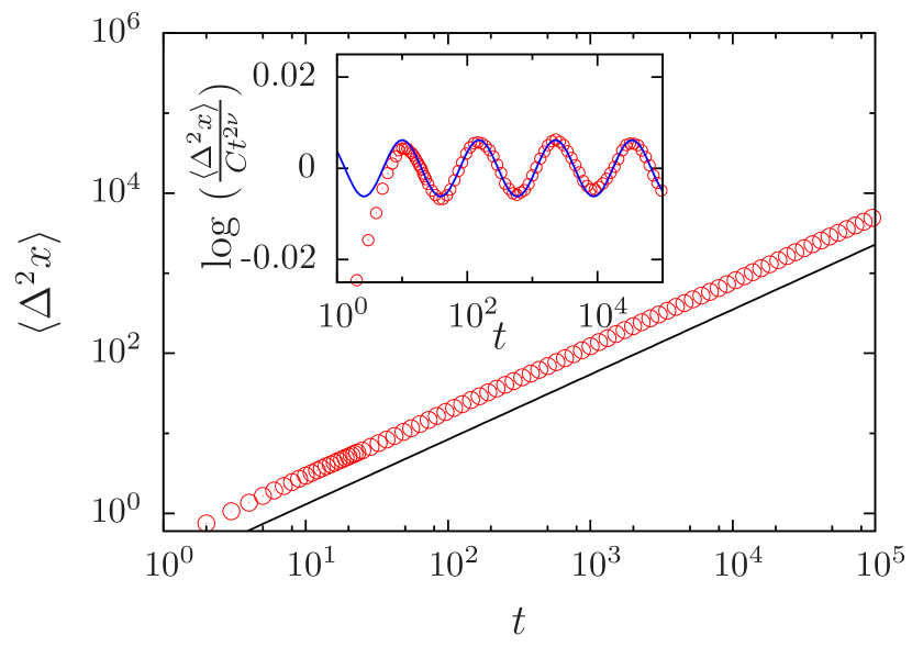
Figure 5: The mean-square displacement $\displaystyle\langle\Delta^{2}x\rangle$ as a function of time for Model I. The straight line has a slope $2\nu$, with $\nu\simeq 0.4057$ obtained from Eq. (10). The inset shows a plot of $\displaystyle\log\langle\Delta^{2}x\rangle/Ct^{2\nu}$ vs. $\log t$ for the same data, where $C$ is a properly chosen constant. The curvilinear line represents the first-harmonic approximation $A\sin(2\pi\log t)/\log(\tau)+\alpha)$. The period $\tau$ is given by Eq.(9). $A$ and $\alpha$ are fitted constants.

The numerical results for the mean-square displacement are plotted as a function of time in Figs. 5 and 6 for Model I and Model II, respectively. It is apparent from these figures that $\displaystyle\langle\Delta^{2}x\rangle(t)$ satisfies a modulated power law. The modulations are more easily observed in each inset, where $\displaystyle\log(\langle\Delta^{2}x\rangle/Ct^{2\nu})$ versus $\log(t)$, is plotted using the same data as in the corresponding main plot ($C$ is a constant chosen to have the oscillations centered around zero). In the case of Model I, the value of the RW exponent ($\nu=0.4057)$ was computed from Eq. (10), while for Model II it was numerically fitted ($\nu_{fit}=0.385$). Note that, in the last case, the value is very close to the analytical approximation $\nu_{1}=0.3846$, indicating that the convergence of the sequence is quite fast. The curvilinear lines are of the form $\displaystyle A\sin(2\pi\log(t)/\log(\tau)+\alpha)$, i. e., the first-harmonic approximation of a periodic function with period $\log(\tau)$, where $A$ and $\alpha$ are fitted parameters. From these figures it is indeed clear that the predictions in Eqs. (9), (10), (14) and (15) are consistent with the numerical findings. Note also that the amplitude of the oscillations is larger in the case of Model II, consistent with its higher value of $\delta$.

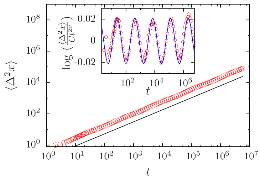
Figure 6: Log-log plot of the mean-square displacement versus time for Model II. The straight line has a numerically fitted slope $2\nu=0.77$. The inset is a plot $\displaystyle\log\langle\Delta^{2}x\rangle/Ct^{2\nu}$ for the same data and the curvilinear line was obtained as in Fig. 5. The period $\tau$ is here obtained from Eq. 9 with the numerical value of $\nu$ ($\nu_{fit}$).

IV Conclusions and discussion

We have studied the time evolution of a single RW on a self-similar finitely ramified structure. The arguments employed in this work show that the time-modulated oscillatory behavior these systems exhibit originates from finite ramification.

Schematically, at a length $L^{n}$, the characteristic unit cell may be visualized as a cage with a given number of gates. While, inside the cage, the RW evolves normally, the situation is significantly different in the border, where the diffusive motion is effectively slowed down due to the small number of gates. A relevant parameter is the ratio between the number of gates and the cage perimeter. Because of finite ramification and self-similarity, this ratio decreases as $n$ increases, and thus, the larger the cage, the harder it will be for the RW to find a way to get out.

The RW dynamics can thus be interpreted as a sequence of normal diffusion behaviors, each characterized by a diffusion coefficient, which decreases as the length-scale increases. The oscillatory modulation amplitude of the mean-square displacement is thus an emergent property of the transitions between two normal diffusion regimes. Because of the substrate self-similarity, the oscillatory behavior survive in the long-time limit.

We have shown that there exist two wide classes of self-similar finitely ramified structures. For pedagogical reasons, we have illustrated their properties by studying two models: the snowflake fractal (Model I) and a (trivial) fractal with a fractal dimension equal to two (Model II). We say that Model I is perfect diffusive self-similar because, on this substrate, a single RW follows, at all time-scales, a power law modulated by log-periodic oscillations. In contrast, we say that Model II is asymptotically diffusive self-similar since, in this case, the log-periodic modulated power law regime is only reached for long enough times. For Model I we have obtained analytically both the global RW exponent and the period of the oscillations. Instead, for Model II, we have shown that a convergent sequence of local exponents and periods exists, and have calculated its first few elements. To check the validity of our approach, MC simulations, were also carried out for each model. The numerical results confirm our theoretical predictions.

We would like to stress that the (nontrivial) fractal character of the substrate is not a necessary condition for anomalous sub-diffusion modulated by log-periodic oscillations. It is a general belief that, in a fractal, a RW becomes sub-diffusive because of the holes of all sizes, which hinder access to some regions. However, we have found a structure (Model II) without those holes but leading to sub-diffusion.

Let us finally observe that, so far, we have considered RWs that always start at the center of symmetry of the structure. However, as shown elsewhere lore2 , for long enough times, the diffusion became independent of the initial position, and the qualitative behavior of Fig. 3 will hold for $L^{n}\gg\ell$, where $\ell$ is the distance between the initial position and that center.

In summary, for a large set of substrates, we have found that the RW sub-diffusive behavior modulated by a log-periodic amplitude can be viewed as an emergent property of self-similarity and finite ramification.

This work was supported by the Universidad Nacional de Mar del Plata and the Consejo Nacional de Investigaciones Científicas y Técnicas (CONICET).

References

- (1) Alexander S. Orbach R., J. Phys. (France) Lett. 43, L625 (1982).
- (2) Rammal R. Toulouse G., J. Phys. (France) Lett. 44, L13 (1983).
- (3) Ben Avraham D. Havlin S., Diffusion and Reactions in Fractals and Disordered Media, Cambridge University Press, Cambridge (2000).
- (4) S. Havlin and D. Ben-Avraham, Adv. Phys. 36, 695 (1987).
- (5) J-P. Bouchaud and A. Georges. Phys. Rep. 195, 127 (1990).
- (6) Grabner P. J. and Woess W., Stochastic Process. Appl. 69, 127 (1997).
- (7) Krön B. and Teufl E. , Trans. Amer. Math. Soc. 356, 393 (2003).
- (8) Acedo L. and Yuste S. B., Phys. Rev. E 63, 011105 (2000).
- (9) Bab M. A., Fabricius G. and Albano E. V., Europhys. Lett. 81, 10003 (2008).
- (10) Bab M. A., Fabricius G. and Albano E. V., J. Chem. Phys. 128, 044911 (2008).
- (11) A. L. Maltz, G. Fabricius, M. A. Bab and E. V. Albano, J. Phys. A: Math. Theor. 41, 495004 (2008).
- (12) Bernasconi J. , Schneider W. R., J. Stat. Phys 30, 355 (1983).
- (13) Stauffer D. Sornette D., Physica A 252, 271 (1998).
- (14) Stauffer D., Physica A 266, 35 (1999).
- (15) Zhang Yu-Xia, Sang Jian-Ping, Zou Xian-Wu, Jin Zhun-Zhi, Physica A 350, 163 (2005).
- (16) Huang Y., Saleur H., Sammis C. Sornette D., Europhys. Lett. 41, 43 (1998).
- (17) Saleur H., Sammis C. G., Sornette D., J. Geogphys. Res. 101, 17661 (1996).
- (18) Krawiecki A., Kacperski K., Matyjaśkiewicz S., Hołyst J. A., Chaos, Solitons and Fractals, 18, 89 (2003).
- (19) Kutnjak-Urbanc Brigita, Zapperi Stefano, Milos̆ević Sava, and Stanley H. Eugene, Phys. Rev. E 54, 272 (1996).
- (20) Andrade R. F. S., Phys. Rev. E 61, 7196 (2000).
- (21) M. A. Bab, G. Fabricius E. V. Albano, Phys. Rev. E 71, 36139 (2005).
- (22) Saleur H. Sornette D., J. Phys. I (France) 6, 327 (1996).
- (23) Sornette D.,Johansen A., Arneodo A., Muzy J.-F. Saleur H., Phys. Rev. Lett 76, 251 (1996).
- (24) Huang Y., Ouillon G., Saleur H. Sornette D., Phys. Rev. E 55, 6433 (1997).
- (25) Sornette D., Johansen A. Bouchaud J-P., J. Phys. I (France) 6, 167 (1996).
- (26) Vanderwalle N., Boveroux Ph., Minguet A., Ausloos M., Physica A 255, 201 (1998).
- (27) Vanderwalle N., Ausloos M., Eur. J. Phys. B 4, 139 (1998).
- (28) Vanderwalle N., Ausloos M., Boveroux Ph., Minguet A., Eur. J. Phys. B 9, 355 (1999).
- (29) Douçot B., Wang W., Chaussy J., Pannetier B., Rammal R., Vareille A., and Henry D., Phys. Rev. Lett. 57, 1235 (1986).
- (30) Sornette D., Phys. Rep. 297, 239 (1998).
- (31) L. Padilla, H. O. Mártin and J. L. Iguain, EPL 85, 20008 (2009).
- (32) T. Vicsek, Fractal Growth Phenomena (2nd Edition), World Scientific, Singapore (1992).
- (33) Aldao C. M., Iguain J. L. and Mártin H. O., Surf. Sci 366, 483 (1996).
- (34) A similar behavior can be observed in figure 7 of Ref.lore1 .