Querying for the Largest Empty Geometric Object in a Desired Location

Abstract

We study new types of geometric query problems defined as follows: given a geometric set $P$, preprocess it such that given a query point $q$, the location of the largest circle that does not contain any member of $P$, but contains $q$ can be reported efficiently. The geometric sets we consider for $P$ are boundaries of convex and simple polygons, and point sets. While we primarily focus on circles as the desired shape, we also briefly discuss empty rectangles in the context of point sets.

1 Introduction

Largest empty space recognition is a classical problem in computational geometry, and has applications in several disciplines like data-mining, database management, VLSI design, to name a few. Here the problem is to identify an empty space of desired shape and maximum size in a given region containing a given set of obstacles. Given a set $P$ of points in $\mathbb{R}^{2}$, an empty circle, is a circle that does not contain any member of $P$. An empty circle is said to be a maximal empty circle (MEC) if it is not fully contained in any other empty circle. Among the MECs’, the one having maximum radius is the largest empty circle. The largest empty circle among a point set $P$ can easily be located by using the Voronoi diagram of $P$ in $O(n\log n)$ time [25]. The maximal empty axis-parallel rectangle (MER) can be defined in a similar manner. The literature on recognizing the largest empty axis-parallel rectangle among obstacles has spanned over three decades in computational geometry. The pioneering work on this topic is by Namaad et al. [20] where it is shown that the number of MERs’ ($m$) among a set of $n$ points may be $O(n^{2})$ in the worst case. In the same paper, an algorithm for identifying the largest MER was proposed. The worst case time complexity of that algorithm is $O(min(n^{2},m\log n))$. The best known result on this problem runs in $O(n\log^{2}n)$ time in the worst case. The same time complexity result holds for the recognition of the largest MER among a set of arbitrary polygonal obstacles [21]. However, the largest MER inside an $n$-sided simple polygon can be identified in $O(n\log n)$ time [5]. The worst case time complexity for recognizing the largest empty rectangle of arbitrary orientation among a set of $n$ points is $O(n^{3})$ [9].

Although a lot of study has been made on the empty space recognition problem, surprisingly, the query version of the problem has not received much attention to the best of our knowledge. The problem of finding the largest empty circle centered on a given query line segment has been considered in [4]. The preprocessing time, space and query time of the proposed algorithm are $O(n^{3}\log n)$, $O(n^{3})$ and $O(\log n)$, respectively. In practical applications, one may need to locate the largest empty space of a given shape in a desired location. For example, in the VLSI physical design, one may need to place a large circuit component in the vicinity of some already placed components. Such problems arise in mining large data sets as well, where the objective is to quickly study the characteristics (such as the area of the empty space) near a query point.

In this paper, we will study the query versions of the empty space recognition problem. If the desired object is a circle, the problem is referred to as maximal empty circle query (QMEC) problem, and if the desired object is an axis-parallel rectangle, the problem is referred to as maximal empty rectangle query (QMER) problem. The following variations are considered.

Given a convex polygon $P$, preprocess it such that given a query point $q$, the largest circle inside $P$ that contains the query point $q$ can be identified efficiently.

Given a simple polygon $P$, preprocess it such that given a query point $q$, the largest circle inside $P$ that contains the query point $q$ can be identified efficiently.

Given a set of points $P$, preprocess it such that given a query point $q$, the largest circle that does not contain any member of $P$, but contains the query point $q$ can be identified efficiently.

Given a set of points $P$, preprocess it such that given a query point $q$, the largest rectangle that does not contain any member of $P$, but contains the query point $q$ can be identified efficiently.

We believe that our work motivates study of new types of geometric query problems and may lead to a very active research area. The main theme of our work is to mainly understand which problems can be solved in subquadratic preprocessing time and space, while ensuring polylogarithmic query times. Our results are summarized in Table 1.

Table 1: Complexity results of different variations of largest empty space query problem

Geometric set	Shape of	Preprocessing	Space	Query time	Sections
	empty space	time
Convex Polygon	circle	$O(n)$	$O(n)$	$O(\log n)$	3
Simple Polygon	circle	$O(n\log^{3}n)$	$O(n\log^{2}n)$	$O(\log^{2}n)$	4
Point Set	circle	$O(n^{2}\log n)$	$O(n^{2})$	$O(\log n)$	5
Point Set	rectangle	$O(n^{2}\log n)$	$O(n^{2}\log n)$	$O(\log n)$	6

In the course of studying these problems, we developed two different ways of implementing a key data structures for storing $n$ circles of arbitrary sizes such that when a query point $q$ is given, it can report the largest of the circles that contains $q$. This data structure may be of independent interest since it may aid in several other geometric search problems.

2 Preliminaries: LCQ-problem

In this section, we want to build a data structure called the largest circle query data structure (LCQ, in short) for the point location in an arrangement of circles. Our input is a set ${\cal{C}}=\{C_{1},C_{2},\ldots,C_{n}\}$ of circles in non-increasing order of their radii. In the preprocessing phase we will construct the data structure. When a query point $q$ is given, it must report the largest circle in ${\cal{C}}$ that contains $q$ or a null value if $q$ is not enclosed by any circle in ${\cal{C}}$. For simplicity, we assume that at most two circles intersect at any point on the plane.

We provide two ways of building the LCQ data structure. The first method uses divide-and-conquer, leading to a solution that is optimized for preprocessing time. The second method uses a line sweeping technique similar to [24], and it gives a solution with better query time. The complexity results are given in Table 2

Table 2: Table comparing the two solutions for LCQ

Techniques	Preprocessing time	Space	Query time
Divide-and-conquer	$O(n\log^{2}n)$	$O(n\log n)$	$O(\log^{2}n)$
Line sweep	$O(n^{2}\log n)$	$O(n^{2})$	$O(\log n)$

2.1 A divide-and-conquer solution

Preprocessing: We form a tree ${\cal{D}}$ of depth $O(\log n)$ as follows. Its root $r$ represents all the members in $\cal C$, and is attached with a data structure ${\tt vor}(r)$ with the circles in ${\cal C}(r)={\cal C}$. The two children of root, say ${\cal{D}}_{\ell}$ and ${\cal{D}}_{r}$, represent the sets ${\cal C}(r_{\ell})=\{C_{1},C_{2},\ldots,C_{\lfloor\frac{n}{2}\rfloor}\}$ and ${\cal C}(r_{r})=\{C_{\lfloor\frac{n}{2}\rfloor+1},\ldots,C_{n-1},C_{n}\}$, respectively. These define the associated structures ${\tt vor}(r_{\ell})$ and ${\tt vor}(r_{r})$ of ${\cal{D}}_{\ell}$ and ${\cal{D}}_{r}$ respectively. The subtrees of ${\cal{D}}_{\ell}$ and ${\cal{D}}_{r}$ are defined recursively in the similar manner. Finally, the leaves of ${\cal{D}}$ contain $C_{1},C_{2},\ldots,C_{n}$, respectively. The tree is computed in a bottom-up fashion starting from the leaves. The task of the data structure ${\tt vor}(v)$ associated to a node $v$ is to efficiently report whether or not the query point $q$ lies inside the union of the circles in ${\cal C}(v)$ it represents. We will use Voronoi diagram in Laguerre geometry of the circles in ${\cal C}(v)$ [15]. Each cell of this Voronoi diagram is a convex polygon and is associated with a circle in ${\cal C}(v)$. The membership query is answered by performing a point location in the associated planar subdivision. For a node $v$, ${\tt vor}(v)$ can be computed in $O(|C(v)|\log|C(v)|)$ time and membership query can be answered in $O(\log|C(v)|)$ time [15].

Query answering: To find the largest circle in $C_{q}$ containing the given query point $q$, we start searching from the root $r$ of ${\cal{D}}$. If $q$ does not lie in the union of circles ${\cal C}(r)=\cal C$, then $q$ is contained in an empty circle of size infinity. We need not proceed further in the tree. However, if the search succeeds, we need to continue the search among its children. A successful search at a node $v$ indicates that $q$ must lie either in the union of circles of its left child or the right child or both. We first consider its left child $v_{\ell}$, that contains the larger $\frac{|{\cal C}(v)|}{2}$ circles of node $v$. We search in the associated structure ${\tt vor}(v_{\ell})$. If the search succeeds (i.e., $q\in\cup_{C\in{\cal C}(v_{\ell})}C$), the search proceeds in the subtree rooted at $v_{\ell}$. However, if the search fails, surely $q$ lies in the union of circles ${\cal C}(v_{r})$, and the search proceeds in the subtree rooted at $v_{r}$. Proceeding similarly, one can identify the largest circle $C_{q}$ containing the query point $q$.

Theorem 2.1

A set $\cal C$ of $n$ circles can be preprocessed in $O(n\log^{2}n)$ time and $O(n\log n)$ space so that LCQ queries can be answered in $O(\log^{2}n)$ time.

2.2 A line sweep solution

We assume a pair of orthogonal lines on the plane to represent the coordinate system. The circles are given as a set of tuples; each tuple representing a circle consists of the coordinates of its center and the radius of that circle. The ordered set of vertices $V=(v_{1},v_{2},\ldots,v_{|V|})$ of the arrangement ${\cal A}({{\cal{C}}})$ consists of the (i) leftmost and rightmost point of each circle in ${\cal{C}}$, and (ii) points in which a pair of circles intersect. We assume, further, that the vertices of ${\cal A}({{\cal{C}}})$ have unique $x$ coordinates, thereby allowing the elements of $V$ to be stored in increasing order of their $x$ coordinates. A maximal segment of any circle in ${\cal{C}}$ that does not contain a vertex is called an edge of ${\cal A}({{\cal{C}}})$. We use $E$ to denote the set of all edges of ${\cal A}({{\cal{C}}})$. Since we include the left and right extremeties of a circle in the set of vertices, the edges are always $x$-monotone. Each edge is attached with two fields $ID_{1}$ and $ID_{2}$ indicating the largest circle containing the cell above and below it respectively. Each cell is bounded by the edges of ${\cal A}({{\cal{C}}})$, and is attached with an index $ID$ indicating the largest circle containing that cell. We compute the arrangement ${\cal A}({{\cal{C}}})$ as follows:

Step-1

Cut each circles into pseudo-segments such that a pair of pseudo-segments intersect in at most one point. If any of these segment contains the leftmost/rightmost point of the corresponding circle, it is again split at that point.

Step-2

Sweep a vertical line from left to right to compute the cells of the arrangement ${\cal A}({{\cal{C}}})$. We also compute the $ID$ field of each cell during the sweep.

Step-1

Consider a circle $C_{i}\in{\cal{C}}$. Each circle $C_{j}\in{\cal{C}}$, $j\neq i$, creates an arc $\alpha_{j}^{i}$ along the boundary of $C_{i}$ that indicates the portion of the boundary of $C_{i}$ that is inside $C_{j}$. In order to split $C_{i}$ into pseudo segments, we need to compute the minimum number of rays from the center of $C_{i}$ that are required to pierce all the arcs $\alpha_{j}^{i}$, $j=1,2,\ldots,n$, $j\neq i$. This can be computed using the $O(n)$ time algorithm for computing the minimum geometric clique cover of the circular arc graph provided the end-points of the circular arcs are sorted [14]. But, we need to sort the end-points of the circular arcs along the boundary of $C_{i}$. Thus, the splitting of all the circles in ${\cal{C}}$ into pseudo segments need $O(n^{2}\log n)$ time. Tamaki and Tokuyama [26] showed that the number of pseudo segments may be $O(n^{\frac{5}{3}})$ in the worst case. Recently Aronov and Sharir [3] showed that number of pseudo-segments generated from $n$ unequal circles is at most $n^{\frac{3}{2}+\epsilon}$, where $\epsilon$ can be made arbitrarily small.

Step-2

In this step, we sweep a vertical line from left to right exactly as in [17] to compute the arrangement ${\cal A}({\cal{C}})$. During the sweep, four types of events may occur: (i) leftmost point of a circle (ii) rightmost point of a circle, (iii) an end-point of a pseudo-segment that is not of type (i) or type (ii), and (iv) intersection point of two pseudo-segments. The events of type (i), (ii) and (iii) are initially inserted in a heap $\cal H$. The events of type (iv) are inserted in $\cal H$ when these are observed during the sweep. The sweep line status data structure ${\cal L}$ stores the edges intersected by the sweep line at the current instant of time. Each pair of consecutive edges indicate a cell intersected by the sweep line. Each cell $\eta$ intersected by the sweep line (indicated by a pair of consecutive edges in the sweep line status) is attached with a balanced binary search tree $\tau_{\eta}$ containing the radii of the circles overlapping on that cell. Each time an event having minimum $x$-coordinate is chosen from $\cal H$ for the processing. The actions taken for each type of event is listed below.

$\bullet$

While processing a type (i) event corresponding to a circle $C$, a new cell $\eta$ and two new edges, say $e_{1}$ and $e_{2}$, of ${\cal A}({{\cal{C}}})$ take birth. These two new consecutive edges are inserted in ${\cal L}$. If the new cell $\eta$ arrives inside an existing cell $\eta^{\prime}$ in the sweep line status $\cal L$, then $\tau_{\eta}$, attached to the cell $\eta$, is created by copying $\tau_{\eta^{\prime}}$ and inserting the radius of the circle $C$ in it. The $ID$ field attached with the cell $\eta$ is the largest element in $\tau_{\eta}$.

$\bullet$

Type (ii) events are also handeled in a similar fashion. Here two edges are deleted from the sweep line status $\cal L$. Thus, a cell will also disappear from $\cal L$.

$\bullet$

At a type (iii) event one edge leaves the sweep-line and a new edge appears on the sweep line. Here, excepting this change on the sweep line, no other action is needed.

$\bullet$

While processing a type (iv) event, an old cell $\eta^{\prime}$ disappears from the sweep line and a new cell $\eta$ takes birth. If the event is generated due to the intersection of edges $e_{1}$ and $e_{2}$ corresponding to the circles $C_{1}$ and $C_{2}$, then $\tau_{\eta}$ is obtained by doing an $O(\log n)$ time updating of $\tau_{\eta^{\prime}}$. If $\eta$ is inside (resp. outside) of the circle $C_{i}$, then the radius of $C_{i}$ is inserted in (resp. deleted from) $\tau_{\eta^{\prime}}$ to get $\tau_{\eta}$. Finally, the largest element of $\tau_{\eta}$ is attached as the $ID$ field of the cell $\eta$.

Since the number of type (i) events is $O(n)$, and each type (i) event needs $O(n)$ time (for copying a heap for the new cell), the time needed for processing all type (i) events is $O(n^{2})$ in the worst case. The number of type (ii) and type (iii) events are $O(n)$ and $O(n^{\frac{5}{3}})$ respectively. As mentioned above, processing each type (ii)/type (ii) event needs $O(1)$ time. The number of type (iv) events is $O(n^{2})$ in the worst case, and their processing needs $O(n^{2}\log n)$ time. The point location in the arrangement ${\cal A}({\cal{C}})$ of pseudo-segments is similar to that in the arrangement of line-segments. Using trapezoidal decomposition of cells, one can perform the query in $O(\log n)$ time [23]. Thus, we have the following result:

Theorem 2.2

Given a set of circles of arbitrary radii, the preprocessing time and space complexity of the LCQ data structure are $O(n^{2}\log n)$ and $O(n^{2})$ respectively, and given an arbitrary query point, the largest circle containing it can be reported in $O(\log n)$ time.

3 QMEC problem for convex polygon

Let $P$ be a convex polygon and $\{p_{1},p_{2},\ldots,p_{n}\}$ be its vertices in anticlockwise order. The objective is to preprocess $P$ such that given an arbitrary query point $q$, the largest circle $C_{q}$ that contains $q$ but not intersected by the boundary of $P$ can be reported efficiently. Needless to say, if $q$ lies outside or on the boundary of $P$, $C_{q}$ is a circle of infinite radius passing through $q$. So, the interesting problem is the case where $q$ lies inside $P$. Needless to mention that here $C_{q}$ is an MEC inside $P$. The medial axis $M$ of $P$ is the locus of the centers of all the MECs’ inside $P$. Let $c$ be the center of the largest MEC inside $P$ (see Figure 1(a)). The medial axis consists of straight line segments and can be viewed as a tree rooted at $c$ [10]. To avoid the confusion with the vertices of the polygon, we call the vertices of $M$ as nodes. Note that, the leaf-nodes of $M$ are the vertices of $P$. Let us denote an MEC of $P$ centered at a point $x\in M$ as $MEC_{x}$ and let $A_{x}$ be the area of $MEC_{x}$.

Figure 1: (a) Illustration of Observation 1, and (b) Partition of $P$.

Observation 1

As the point $x$ moves from $c$ along the medial axis towards any vertex $p_{i}\in P$ (leaf node of $M$), $A_{x}$ decreases monotonically (see Figure 1(a)).

Proof

Follows from the convexity of the polygon $P$. ∎

The medial axis $M$ partitions the polygon $P$ into $n$ convex sub-polygons such that each sub-polygon $P_{i}$ consists of a polygonal edge $p_{i}p_{i+1}$ and two convex chains of $M$, one starting at $p_{i}$ and other starting at $p_{i+1}$ (see Figure 1(b)). This partitioning can be achieved in $O(n)$ time since $M$ can be computed in linear time [10]. Moreover, $M$ can be preprocessed in $O(n)$ time so that the sub-polygon containing any query point $q$ can be located in $O(\log n)$ time [18].

Lemma 1

The polygon $P$ can be partitioned in $O(n)$ time such that given any arbitrary query point $q$, the edge of $M$ closest to $q$ can be reported in $O(\log n)$ time.

Proof

We consider each $P_{i}$ separately, and compute the medial axis of the convex chain from $p_{i}$ to $p_{i+1}$ (a portion of $M$). This needs $O(\mu_{i})$ time [1], where $\mu_{i}$ is the number of nodes in $M$ that appear as the vertices of $P_{i}$. Thus, for the entire polygon $P$, the total time complexity is $O(\sum_{i=1}^{n}\mu_{i})=O(n)$, since the number of edges of $M$ is $O(n)$, and each edge of $M$ appears in exactly two sub-polygons. If the query point $q$ appears in $P_{i}$, then we can locate the edge of $M$ that is closest to $q$ in $O(\log\mu_{i})$ time using point location in planar subdivision [18]. ∎

Now we will describe how to solve the QMEC problem for a convex polygon. Assume that the query point $q$ lies inside the sub-polygon $P_{i}$, that is incident to the edge $p_{i}p_{i+1}$ of $P$. Let $c^{\prime}$ denote the center of the largest MEC containing $q$. Note that, $c^{\prime}$ will lie either on the path from $p_{i}$ to $c$ (denoted by $p_{i}\sim c$) or on the path from $p_{i+1}$ to $c$ ($p_{i+1}\sim c$) on $M$. Let us assume that $c^{\prime}$ lie on the path $p_{i}\sim c$. We use Lemma 1 to identify a point $x$ on the path $p_{i}\sim c$ that is closest to $q$ in $O(\log n)$ time. The $MEC_{x}$ must contain $q$.

By Observation 1, we can locate $c^{\prime}$ by performing a binary search on the path $c\sim x$ that finds two consecutive nodes $v$ and $v^{\prime}$ on the path such that $MEC_{v}$ encloses $q$, but $MEC_{v^{\prime}}$ does not. In degenerate case $v$ may be $x$ and $v^{\prime}$ is its previous node on the path $c\sim x$. Since the path lies on a tree representing the medial axis $M$, we can use level-ancestor queries [6] for this purpose. After computing $v$ and $v^{\prime}$, the exact location of $c^{\prime}$ can be determined in $O(1)$ time. Thus, we have the following theorem:

Theorem 3.1

A convex polygon on $n$-vertices can be preprocessed in $O(n)$ time and space so that the QMEC queries can be answered in $O(\log n)$ time.

4 QMEC problem for simple polygon

Our approach for solving the QMEC problem in a simple polygon $P$ is based on the divide and conquer strategy, and it uses the tree structure of the medial axis $M$. Here again the leaf nodes correspond to the vertices of the polygon. The internal nodes correspond to the points on $M$ such that the MEC centered at each of those points touches 3 or more distinct points on the boundary of $P$; We use ${\cal{N}}$ to denote the set of internal nodes of $M$.

For the sake of simplicity in analyzing the algorithm, we assume that the MECs centered at the internal nodes of $M$ have distinct radii. A point $x\in M$, that is not a leaf, is said to be a valley point if for a sufficiently small $\delta>0$, the MECs centered at points in $M$ within a distance $\delta$ from $x$ are at least as large as $MEC_{x}$. We can similarly define the peaks in $M$. We assume that the number of peaks and valley points are finite. We use $\Phi$ and $\Theta$ to denote the set of valleys and peaks respectively. It is easy to observe that $\Phi\cap{\cal{N}}=\emptyset$, but $\Theta\subseteq{\cal{N}}$.

Finally, we define a mountain to be a maximal subtree of $M$ that does not contain any valley point except its leaves. Notice that,

• Each mountain has exactly one peak.

• Each valley point is common to exactly two mountains, and it is a leaf for both the mountains.

• If a point $x$ proceeds from a valley point of a mountain toward its peak, the size of $MEC_{x}$ increases.

Thus, if we partition $M$ by cutting the tree at all the valley points, we get a set of mountains ${\cal{M}}=\{M_{1},M_{2},\ldots,M_{|{\cal{M}}|}\}$ (See Figure 2(a)).

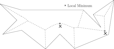
(a)

(b)

Figure 2: (a) Partitioning the medial axis $M$, and (b) The subtree $M^{q}$ for a query point $q$

We also need to consider another way of splitting the tree $M$ as stated in Lemma 2. This aids in designing a data structure ${\cal{T}}$ for the query algorithm.

Lemma 2

[16] Every tree $T$ with $n$ nodes has at least one node $\pi$ whose removal splits the tree into subtrees with at most $\lceil\frac{n}{2}\rceil$ nodes. The node $\pi$ is called the centroid of $T$.

Lemma 3

If $q$ is the query point and $M^{q}$ is the maximal portion of $M$ such that MECs centered in any point on $M^{q}$ enclose the query point $q$, then $M^{q}$ is a connected subtree of $M$ (see Figure 2(b)).

Lemma 4

If $q$ falls outside the $MEC_{\pi}$, then $M^{q}$ is contained entirely in one of the subtrees obtained by deleting $\pi$ from $M$.

Proof

Follows from the connectedness of $M^{q}$ (see Lemma 3). ∎

Lemmata 3 and 4 lead to the following divide and conquer algorithm for the QMEC problem for a simple polygon.

In the preprocessing phase, we first compute the medial axis $M$. Next, we create a tree ${\cal{T}}$ whose root node is the centroid $\pi$ of $M$. The children of the root node in ${\cal{T}}$ are the centroids of the subtrees obtained by deleting $\pi$ from $M$. The process continues up to the leaf level. Each node $v\in{{\cal{T}}}$ is attached with $MEC_{v}$. Note that, the MEC attached to the root node of ${\cal{T}}$ may not be the largest MEC in $P$.

During the query with a point $q$, we need to consider two cases: (i) $q$ lies inside the $MEC_{v}$ for some vertex $v$ of the medial axis $M$, and (ii) $q$ does not lie in the MEC of any vertex of the medial axis. We describe the method of computing $C_{q}$ in Case (i). In Case (ii) (i.e., where Case (i) fails), then we identify the mountain $M_{i}$ in which $q$ lies. Next, we find $C_{q}$ in $M_{i}$ using the same method as in the Convex polygon Case, described in Section 3.

The method of solving Case (i) is as follows. We test whether $q$ lies in the MEC attached to the root node of ${\cal{T}}$. If so, we report the largest MEC $C_{q}$ using a data structure Query-in-Circle (or QiC in short), described below. If $q$ does not lie in the MEC corresponding to the root node, then by Lemma 4, we need to search one of the subtrees of the root node. The search process continues until a node $v^{\prime}$ of ${\cal{T}}$ is identified such that $MEC_{v^{\prime}}$ contains $q$.

During the search in the tree ${\cal{T}}$, suppose we have identified a node $v$ such that $q$ lies inside $MEC_{v}$. Thus, $v$ lies on the subtree $M^{q}$. Here two important things need to be noted: (i) $C_{q}$ may not be equal to $MEC_{v}$; it may be some other MEC of larger area centered on $M^{q}$, and (ii) $M^{q}$ may consist of several mountains, The task of the QiC data structure attached to a node $v$ of ${\cal{T}}$ is to identify the appropriate mountains in $M^{q}$ for searching the center of $C_{q}$. We also need another data structure, called MEC-in-Mountain (or MiM in short) that can report the largest MEC containing $q$ with center on a given mountain $M_{i}\in{\cal M}$, provided $M_{i}\cap M^{q}\neq\emptyset$. We now explain MiM and QiC procedures in detail, and then the divide and conquer procedure.

4.1 MiM query

Here we are given the polygon $P$ and a mountain $M_{i}$; we need to report the largest MEC centered at a point on $M_{i}$ provided $M_{i}\cap M^{q}\neq\emptyset$. Note that, if the center moves from any point $x\in M_{i}\cap M^{q}$ to the peak of $M_{i}$, the MECs’ are strictly increasing. Thus, we can apply the algorithm proposed in Section 3 to identify the largest $MEC$ containing $q$, and centered on $M_{i}\cap M^{q}$. The preprocessing time and space complexities are both $O(|M_{i}|)$, and the query time is $O(\log|M_{i}|)$, where $|M_{i}|$ denotes the number of sides of the simple polygon that induces the edges of $M_{i}$.

4.2 QiC query

Here we want to solve a subproblem in which we know that the query point $q$ falls inside an MEC centered at a given point $v\in M$. We are to preprocess this information. In the query phase, given a query point $q\in MEC_{v}$, we are required to report $C_{q}$, the largest MEC containing $q$. This problem is quite challenging since the locus $M_{v}^{*}$ of the center of $C_{q}$ for possible choices of $q$ satisfying above, is a subtree of $M$, and it may span several mountains.

During the breadth-first search in ${\cal{T}}$, suppose we have already identified a vertex $v$ in ${\cal{T}}$ such that $MEC_{v}$ contains the query point $q$. But $C_{q}$ may be some other MEC of larger area. We need to identify $C_{q}$. By Lemma 3, both the center of $C_{q}$ and the node $v$ of ${\cal{T}}$ are guaranteed to be on $M^{q}$.

Let ${\cal{R}}_{v}$ be the set of radii of MECs centered at the internal nodes of the subtree $M_{v}^{*}$ rooted at $v$, sorted in increasing order.

Definition 1

An MEC $C$ is called a guiding MEC corresponding to a node $v$ of $M_{v}^{*}$ if

• its radius is in ${\cal{R}}_{v}$,

• every MEC in the path from $v$ to the center of $C$ (both inclusive) is no larger than $C$, and

• $C$ overlaps with $MEC_{v}$.

Let ${\cal{S}}$ be the set of all guiding MECs of the node $v$. Note that, a member in ${\cal{S}}$ may be centered at the nodes as well as on the edges on $M_{v}^{*}$.

4.2.1 Preprocessing steps in QiC

We perform the following steps in the preprocessing phase to compute ${\cal{S}}$ attached to a node $v$ of $M$. Let $M_{v}^{*}$ be the subtree of $M$ attached to node $v$.

1. Perform a breadth first search in $M_{v}^{*}$ starting at $v$, and it recursively proceeds as follows:

   At each step (at a node $v^{\prime}\in M_{v}^{*}$), if $MEC_{v^{\prime}}$ does not overlap with $MEC_{v}$, the recursion stops along that path; otherwise, two distinct cases need to be considered. We check whether the radii of $MEC_{v^{\prime}}$ and $MEC_{v^{\prime\prime}}$ are consecutive elements in ${\cal{R}}_{v}$, where $v^{\prime\prime}$ is the predecessor node of $v^{\prime}$ in $M_{v}^{*}$.

   • If so, put $MEC_{v^{\prime}}$ in ${\cal{S}}$ and recursively explore all the paths incident at $v^{\prime}$.

   • Otherwise, compute all the MECs with center on the line segment $(v,v^{\prime})$ whose radius matches with the elements in the array ${\cal{R}}_{v}$, put them in ${\cal{S}}$, insert those points on $(v,v^{\prime})$ as the (dummy) nodes in the tree $M$, and then recursively explore all the paths incident at $v^{\prime}$ in $M_{v}^{*}$.

2. Attach the mountain-id with each $C\in{\cal{S}}$. This is available while performing the breath-first search. This will allow us to invoke the MiM query for a particular mountain.

3. Attach each circle in ${\cal{S}}$ with the corresponding mountain in $M$.

4. Create a LCQ data structure with the circles in ${\cal{S}}$, and attach it with node $v$.

Lemma 5

For any $r\in{\cal{R}}_{v}$, the number of circles in ${\cal{S}}$ of radius $r$ attached with node $v$ is bounded by a constant. Furthermore, ${\cal{S}}$ can be computed in $O(|R_{v}|)$ time.

(a)

(b)

Figure 3: (a) Bounding $|{\cal{S}}|$, and (b) Illustration on the number of MECs in ${\cal{S}}_{r}$ that enclose a point $x$

Proof

Consider any $r\in{\cal{R}}_{v}$. Let ${\cal{S}}_{r}$ be the MECs of radius $r$ in ${\cal{S}}$. It suffices to show that $|{\cal{S}}_{r}|$ is bounded by a constant. For convenience, let us assume that ${\cal{S}}_{r}$ does not contain a MEC centered at a node of $M$. This will not affect us because we have assumed that MECs centered at nodes of $M$ have distinct radii, so at most one MEC in ${\cal{S}}_{r}$ can be centered at a node.

Let $r_{v}$ be the radius of $MEC_{v}$ of the root node $v$ of $M_{v}^{*}$. Clearly, $r_{v}\leq r$ (by Definition 1). Also recall that every MEC in ${\cal{S}}$ must (at least tangentially) intersect $MEC_{v}$. See Figure 3(a) for an illustration. Therefore, every MEC in ${\cal{S}}_{r}$ must lie entirely within a circle $\chi$ of radius $r_{v}+2r$ centered at $v$. Thus, we need to prove that the number of guiding circles of radius $r$ at node $v$ inside $\chi$ is bounded by a constant.

Let us consider a point $x\in P$ . Let ${\cal{S}}_{r}^{x}\subseteq{\cal{S}}_{r}$ be a set of MECs that enclose $x$. Let $C$ be any MEC in ${\cal{S}}_{r}^{x}$ and $c$ be its center. Let $p_{1}$ and $p_{2}$ be the two points at which $C$ touches the boundary of the polygon $P$. The chord $[p_{1},p_{2}]$ must intersect the medial axis (see Figure 3(b)). Note that, the points $p$ and $c$ lie in the two different sides of $[p_{1},p_{2}]$. On the contrary, if $p$ and $c$ lie in the same side of $[p_{1}^{\prime},p_{2}^{\prime}]$, where $p_{1}^{\prime}$ and $p_{2}^{\prime}$ are the points of contact of the said MEC and the polygon $P$, then we can increase the size of the MEC by moving its center $c$ towards $p$ along the medial axis (see Figure 3(b)). Thus, $C\not\in{\cal{S}}_{r}$. Thus, we have $\angle p_{1}xp_{2}\geq\pi/2$. These angles subtended by the MECs in ${\cal{S}}_{r}^{x}$ are disjoint implying that $|{\cal{S}}_{r}^{x}|\leq 4$. In other words, any point inside the circle $\chi$ can be enclosed by at most four different circles from ${\cal{S}}_{r}$. We need to compute $|{\cal{S}}_{r}|$. Let us consider a function $f(x)=$ number of circles in ${\cal{S}}_{r}$ that overlaps at the point $x$, $x\in\chi$. $f(x)\leq 4$ for all $x\in\chi$. The total number of circles in ${\cal{S}}_{r}$ can be obtained as follows:

Total area of circles in ${\cal{S}}_{r}\leq\int_{(x,y)\in\chi}f(x)~{}dx~{}dy\leq 4\pi(r_{v}+2r)^{2}$.

Therefore, $|{\cal{S}}_{r}|\leq\frac{4\pi(r_{v}+2r)^{2}}{\pi r^{2}}\leq\frac{4\pi(3r)^{2}}{\pi r^{2}}=36$.

Thus, the first part of the lemma is proved.

The time complexity follows from the fact that the breadth first search in $M_{v}^{*}$ needs $O(|M_{v}^{*}|)$ time. The time for computing the members in ${\cal{S}}$ is $\sum_{r\in{\cal{R}}_{v}}|{\cal{S}}_{r}|=O(|{\cal{R}}_{v}|)$ (by the first part of this lemma). ∎

4.2.2 Query algorithm in QiC

Given a query point $q$, we first traverse the tree ${\cal{T}}$ to identify a node $v$ such that $q\in MEC_{v}$. Note that, the MECs at the nodes of the subtree rooted at $v$ may contain $q$; but the MECs corresponding to all other nodes in ${\cal{T}}$ will not contain $q$ (see Lemma 4). Let ${\cal{S}}$ be the guiding circles attached with node $v$, $\rho\in{\cal{R}}_{v}$ be the radius of the largest guiding circle in ${\cal{S}}$ that contains $q$, and ${\cal{S}}_{q}$ be a subset of ${\cal{S}}$ that has radius $\rho$ and contains $q$. ${\cal{S}}_{q}$ can be obtained from the LCQ data structure attached with node $v$. By Lemma 5, we have $|S_{q}|\leq 36$. In order to report $C_{q}$, we need the following:

Step 1:

an algorithm to identify the mountain associated with each circle in ${\cal{S}}_{q}$,

Step 2:

to locate the largest MEC containing $q$ in each of these mountains using the MiM query algorithm,

Step 3:

to report the largest one among the MECs’ obtained in Step 2 as $C_{q}$.

We first devise an algorithm for Step 1. The necessary algorithm for Step 2 is already available in Subsection 4.1. We then prove the necessary result to ensure the statement stated in Step 3.

Algorithm for Step 1:

Consider a path $\Pi$ from $v$ to a leaf of $M_{v}^{*}$, and observe the size of the MECs’. Figure 4 demonstrates a curve $f(t)$ where $t$ denotes the distance of a point from $v$ on the path $\Pi$, and $f(t)$ denotes the radius of the MEC centered at that point. The guiding circles along the path $\Pi$ correspond to a subsequence of vertices along that path whose corresponding MECs’ are increasing in size.

Lemma 6

The guiding circles along a path $\Pi$ from $v$ to a leaf of $M_{v}^{*}$ containing the query point $q$ appear consecutively along $\Pi$.

Proof

Follows from the connectedness of $M^{q}$ (see Lemma 3). ∎

Consider the MECs’ attached to the nodes in $\Pi$. Let $v^{\prime}$ be such a node whose corresponding MEC is largest among those containing $q$. Let $M^{\prime}$ ($\in{\cal{M}}$) be the mountain in which $v^{\prime}$ lies. Here two cases need to be considered: (i) $v^{\prime}$ is the peak of $M^{\prime}$, and (ii) $v^{\prime}$ is not the peak of $M^{\prime}$. In Case (i), we have already got the largest MEC centered on the path $\Pi$ and containing $q$. In Case (ii), we need to invoke MiM query algorithm to find the largest MEC centered on the mountain $M^{\prime}$.

Correctness of QiC

Lemma 7

At least one of the circles in ${\cal{S}}_{q}$ is centered in the mountain in which $C_{q}$ is centered.

Figure 4: Proof of Lemma 7

Proof

Since $M^{q}$ is a continuous subtree of $M$, if we explore all the paths in $M_{v}^{*}$ from node $v$ towards its leaves, $c_{q}$ is reached in one of such paths, say $\Pi$, and $v^{\prime}$ be a node on $\Pi$ such that the guiding circle $MEC_{v^{\prime}}$ is largest among those which contain $q$. Note that, any point on the path $\Pi$ closer to $v$ than $v^{\prime}$ can not be the center of a larger MEC (see Definition 1). Let the center $c_{q}$ of $C_{q}$ be a point on $\Pi$ that is in a different mountain to the right of $v^{\prime}$. Here again two situations need to be considered: (i) the function $f(t)$ increases monotonically from $v^{\prime}$ to $c_{q}$, and (ii) the function $f(t)$ from $v^{\prime}$ to $c_{q}$ is not monotonic. In Case (i) $v^{\prime}$ and $c_{q}$ lie in the same mountain. In Case (ii), between $v^{\prime}$ and $c_{q}$ there is a point $\alpha$ on the path $\Pi$, such that the radius of $MEC_{\alpha}$ is less than that of $MEC_{v^{\prime}}$. Also, there exists another point $\beta$ on the path $\Pi$ between $\alpha$ and $c_{q}$ such that the radius of $MEC_{\beta}$ is equal to that of $MEC_{v^{\prime}}$. Since the radius of $MEC_{\beta}$ matches with an element of ${\cal{R}}$, $MEC_{\beta}$ is also a guiding circle. Moreover, from the continuity of $M^{q}$, the MEC centered at $\beta$ must contain $q$. So, if $c_{q}$ does not lie in the mountain of $v^{\prime}$, it must lie in the mountain containing $\beta$. Thus, the lemma follows. ∎

Lemma 8

The preprocessing time and space complexities for the QiC query are $O(|M|\log^{2}|M|)$ and $O(|M|\log|M|)$ respectively. Queries can be answered in $O(\log^{2}|M|)$ time.

Proof

Compuing ${\cal{S}}$ requires $O(|M_{v}^{*}|\log|M_{v}^{*}|)$ time because we need to sort the elements in $R_{v}$. The members in ${\cal{S}}$ can be stored in LCQ data structure in $O(|{\cal{R}}_{v}|\log^{2}|{\cal{R}}_{v}|)$ time and $O(|{\cal{R}}_{v}|\log|{\cal{R}}_{v}|)$ space (see Theorem 2.1) and queries can be answered in $\log^{2}|M_{v}^{*}|$.

In the query phase with a query point $q$, we identify a constant number of guiding circles ${\cal{S}}_{q}$ attached to node $v$ that contains $q$. Next, we call MiM queries in their associated mountains; this takes $\log|M_{v}^{*}|$ time (see Theorem 3.1). By Lemma 7, the result of one of the MiM queries will be the largest MEC with center on $M_{v}^{*}$ that contains $q$. Thus the query time complexity follows. ∎

4.3 Query algorithm for finding $C_{q}$

Before we start the divide and conquer, we compute the set ${\cal{M}}$ of mountains and preprocess each of them for MiM query. Since ${\cal{M}}$ is a partition of the medial axis $M$, all the mountains can be preprocessed for MiM query in $O(|M|)$ time. In Lemma 8, it is shown that the total preprocessing time needed for the QiC queries at every node of ${\cal{T}}$ is $O(|M|\log^{2}|M|)$ using $O(|M|\log|M|)$ space.

In the query phase, we start at the root level of ${\cal{T}}$ and check if $q$ falls inside the MEC centered at the root. If yes, we find $C_{q}$ using the query algorithm for QiC. This takes $O(\log^{2}n)$ time (see Lemma 8). Otherwise, we proceed in the appropriate subtree of the root whose corresponding sub-polygon contains $q$. In order to choose this sub-polygon, we need another data structure as stated below.

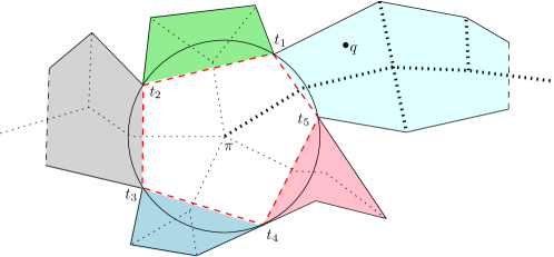
Figure 5: The divide and conquer search structure

Recall that, the medial axis $M$ partitions $P$ into $n$ cells. Let $\pi$ be the centroid node that corresponds to the root of ${\cal{T}}$. Let $\pi$ have $k$ children. In other words, if we consider the $MEC_{\pi}$, it touches $P$ at $k$ different points. This gives birth to $k$ sub-polygons (as illustrated in Figure 5 with $k=5$). The centroid of each sub-polygon is a child of $\pi$. We attach a first-level-tag $i$ with each cell in the $i$-th sub-polygon, for $i=1,2,\ldots,k$. Next, we consider the children of $\pi$ (the nodes in the second level of ${\cal{T}}$) in a breadth first manner. For each sub-polygon, consider its centroid. The MEC of that node again partition that sub-polygon into further parts. We attach a second-level-tag to each cell of that sub-polygon as we did for the root. After considering all the children of $\pi$, we go to the third level, and do the same for attaching the third-level-tag to the partitions of $P$. Since the number of levels of ${\cal{T}}$ is $O(\log n)$ in the worst case, a cell of $P$ may get $O(\log n)$ tags. Thus each cell is attached with an array TAG of size $O(\log n)$ containing tags of $O(\log n)$ levels. This needs $O(n\log n)$ time and space in the worst case.

By point location in the planar subdivision of $P$, we know in which partition $Q$ of $P$ the query point $q$ lies. While searching in the tree ${\cal{T}}$, if $q$ does not lie in $MEC_{u}$ of a node $u$ in the $i$-th level, we choose the appropriate subtree of $u$ by observing the $i$-th entry of the array TAG attached to the partition $Q$, and proceed in that direction. Thus, the overall query time complexity includes (i) $O(\log n)$ for the point location in the subdivision of $P$, (ii) $O(\log n)$ time for traversal in ${\cal{T}}$, (iii) $O(\log^{2}n+K\log n)$ time for identifying the largest guiding circles attached to node $v$ (in its $LCQ$ data structure) if node $v$ is observed first during traversal of ${\cal{T}}$, such that $MEC_{v}$ contains $q$, and the MiM queries for $K$ mountains if $K$ circles are output of step (iii). In Lemma 5, it is proved that $K$ is bounded by a constant. Thus, we have the following theorem.

Theorem 4.1

A simple polygon can be preprocessed in $O(n\log^{3}n)$ time using $(n\log^{2}n)$ space and the QMEC queries can be answered in $O(\log^{2}n)$ time.

5 QMEC for Point Set

The input consists of a set of points $P=\{p_{1},p_{2},\ldots,p_{n}\}$ in $\mathbb{R}^{2}$. The objective is to preprocess $P$ such that given any arbitrary query point $q$, the largest circle $C_{q}$ that does not contain any point in $P$ but contains $q$, can be reported efficiently. Observe that, if $q$ lies outside or on the boundary of the convex hull of $P$, we can draw a circle of infinite radius passing through $q$. So, we shall consider the case where $q$ lies in the proper interior of the convex hull of $P$.

An MEC centered at a Voronoi vertex touches at least three points from $P$. We assume that the MECs centered at Voronoi vertices are of distinct sizes. For our purpose, we also compute some artificial vertices, one on each Voronoi edge that is a half line. We must compute these artificial vertices carefully to ensure that the following conditions hold.

1. Every MEC centered at an artificial vertex must be larger than MECs centered at Voronoi vertices, and

2. the MECs centered at artificial vertices should not overlap pairwise within the convex hull of $P$. Surely, they overlap outside the convex hull of $P$.

The second condition ensures that there exists no query point $q$ which can be enclosed by more than one MEC centered at artificial vertices. This second condition makes the choice of artificial vertices somewhat tricky, but it is a simple exercise to see that we can choose the artificial vertices in $O(n^{2})$ time. We use the unqualified term vertex to refer either to a Voronoi vertex or an artificial vertex.

Now, consider the planar graph with both the Voronoi vertices and the artificial vertices. Let $v$ be a Voronoi vertex and let $MEC_{v}$ be the MEC centered at $v$. A path ${\cal{P}}_{v}=(v^{1}=v,v^{2},\ldots,v^{k})$ from $v$ in the graph is said to be a rising path with respect to $v$ if

• MECs centered at vertices other than $v^{1}$ and $v^{k}$ are strictly smaller than $MEC_{v}$, and

• $MEC_{v^{k}}$ is strictly larger than $MEC_{v}$. Note that $v^{k}$ may be an artificial vertex, but the other vertices in the path ${\cal{P}}_{v}$ are surely Voronoi vertices.

The last edge $(v^{k-1},v^{k})$ is called a rising edge with respect to the vertex $v$. Since $MEC_{v^{k-1}}$ is smaller than $MEC_{v}$, but $MEC_{v^{k}}$ is larger than $MEC_{v}$, there is exactly one MEC centered on the edge $(v^{k-1},v^{k})$ that equals the size of $MEC_{v}$. Let us denote this MEC by $MEC_{{\cal{P}}_{v}}$. If $MEC_{{\cal{P}}_{v}}$ overlaps $MEC_{v}$, then the rising edge $(v^{k-1},v^{k})$ is called an overlapping edge with respect to vertex $v$. Let ${\cal{O}}_{v}$ be the set of overlapping edges with respect to $v$. Observe that ${\cal{O}}_{v}$, for a given vertex $v$, can be computed in $O(n)$ time via a breadth first search from $v$. The preprocessing and query procedures are given in Procedures 1 and 2.

Procedure 1 Preprocessing steps

1:  INPUT: Set of points $P$ in $\mathbb{R}^{2}$.

2:  Compute the MECs centered at (both Voronoi and artificial) vertices, and store them in LCQ data structure.

3:  For each vertex $v$, compute ${\cal{O}}_{v}$ using a breadth first search.

Procedure 2 Query steps

1:  INPUT: a query point $q$ along with the LCQ data structure containing MECs centered at vertices, and ${\cal{O}}_{v}$ for every internal vertex $v$ in the the Voronoi diagram of $P$.

2:  Find the largest MEC $C^{q}$ in the LCQ data structure containing $q$. Let $v^{q}$ be the center of $C^{q}$.

3:  if $v^{q}$ is an artificial vertex then

4:     Report $C_{q}=C^{q}$ as the largest circle containing $q$ that is centered on the edge containing $v^{q}$.

5:     Exit

6:  end if

7:  $C\leftarrow C^{q}$

8:  for all edges $e\in{\cal{O}}_{v^{q}}$ do

9:     if MECs centered on $e$ do not enclose $q$ then

10:        Continue to next edge in $O_{v^{q}}$

11:     end if

12:     Let $C^{e}$ be the largest circle centered on $e$ that encloses $q$.

13:     $C\leftarrow\max(C,C^{e})$

14:  end for

15:  Report $C$

We are now left with showing that Procedures 1 and 2 are correct and bound their complexities. We address the latter first. We begin with a lemma. which can be proved essentially using the proof of Lemma 5.

Lemma 9

For any internal vertex $v$ in the Voronoi diagram of $P$, $|{\cal{O}}_{v}|$ is bounded by a constant.

Proof

Let $MEC_{v}$ be the circle centered on $v$. Consider any overlapping edge $e=(v_{1},v_{2})$ in ${\cal{O}}_{v}$. Assume without loss of generality that the MEC at $v_{2}$ is larger than the MEC at $v_{1}$. By definition, there is a point $v^{\prime}$ on $e$ such that $MEC_{v^{\prime}}$ has the same radius as $MEC_{v}$ and that $MEC_{v^{\prime}}$ intersects $MEC_{v}$. Let $p_{1}$ and $p_{2}$ be the two points in $P$ that touch the MEC at $v^{\prime}$. The chord $p_{1}p_{2}$ intersects the edge $e$ somewhere between $v_{1}$ and $v^{\prime}$ (see Figure 3). Otherwise, the MEC at $v^{\prime}$ will not be the first MEC from $v_{1}$ to $v_{2}$ that equals $MEC_{v}$ in size. Therefore, we can use the same idea from Lemma 5 to bound the number of overlapping edges. ∎

Lemma 10

Given that we can construct the LCQ data structure for $n$ circles in $O(p(n))$ preprocessing time with a space complexity of $O(s(n))$ and queries answered in $O(q(n))$ time, Procedure 1 (for preprocessing) takes $O(p(n)+n^{2})$ time and $O(s(n)+n)$ space, and Procedure 2 (for query answering) takes $O(q(n))$ time.

Proof

The complexity bounds for LCQ data structure are added for the obvious reason that we use the LCQ data structure for creating and storing $O(n)$ MECs centered at the internal vertices of the Voronoi diagram. Line number 3 of Procedure 1 performs $O(n)$ breadth first searches, hence we added an $O(n^{2})$ term to the preprocessing time. As a consequence of Lemma 9, our space requirements is limited to $O(n)$ and, more importantly, the query time does not incur anything more than $q(n)$. ∎

Lemma 11

Consider any cycle $H$ in the Voronoi diagram of $P$. Let $C_{H}$ be any MEC centered at some point on $H$. Then, there exists another MEC $C^{\prime}_{H}$ centered at some other point on $H$ that does not properly overlap $C_{H}$.

Proof

Clearly, any cycle in the Voronoi diagram of $P$ must contain at least one point from $P$ inside it. Let $p\in P$ be such a point that lies inside the cycle $H$ (see Figure 6). Let $C_{H}$ be any MEC centered at some point on $H$; $c_{H}$ be its center. Consider the line connecting $c_{H}$ and $p$. It intersects $H$ at another point $c^{\prime}_{H}$. It is easy to see that the MEC $C_{H}^{\prime}$, centered at $c^{\prime}_{H}$, will not properly overlap with $C_{H}$. Because, in that case $p$ will be properly contained within $C_{H}$ and $C^{\prime}_{H}$.

Figure 6: Illustration of Lemma 11; the edges in $H$ are shown darker

∎

Lemma 12 (Unique Path Lemma)

Let $C$ and $C^{\prime}$ be any two distinct but overlapping MECs with center at $c$ and $c^{\prime}$ respectively. There is exactly one path from $c$ to $c^{\prime}$ along the Voronoi edges such that every MEC centered on that path encloses $C\cap C^{\prime}$.

Proof

The structure of the proof is as follows. We provide a procedure that constructs a path $\Pi(c,c^{\prime})$ from $c$ to $c^{\prime}$ along the Voronoi edges, and ensure that every MEC centered on that path encloses $C\cap C^{\prime}$. As a consequence of Lemma 11, the path does not form an intermediate cycle and terminates at $c^{\prime}$. Finally, we again use Lemma 11 to show that no path ${\cal{P}}$, other than $\Pi(c,c^{\prime})$, exists between $c$ and $c^{\prime}$ such that every MEC centered on ${\cal{P}}$ contains $C\cap C^{\prime}$. Throughout this proof, we closely follow Figure 7 in order to keep the arguments intuitive. To keep arguments simple, we assume that $c$ and $c^{\prime}$ are Voronoi vertices. When $c$ and $c^{\prime}$ are not Voronoi vertices, then also the same argument follows.

Let $\alpha$ be the number of points in $P$ that $C$ touches. These $\alpha$ points partition $C$ into $\alpha$ arcs. The degree of the corresponding Voronoi vertex $c$ is also $\alpha$ because each adjacent pair of points from $P$ that lie on the boundary of $C$ will induce a Voronoi edge incident on $c$ and vice versa. These Voronoi edges and their corresponding arcs are denoted by $e^{j}_{C}$ and $s^{j}_{C}$, for $1\leq j\leq\alpha$.

Consider the other MEC $C^{\prime}$ ($\neq C$ and centered at a vertex $c^{\prime}$) that overlaps with $C$. $C^{\prime}$ intersects $C$ at two points $t_{1}$ and $t_{2}$; both $t_{1}$ and $t_{2}$ must lie in one of the $\alpha$ arcs of $C$ (due to the emptiness of $C^{\prime}$). Let us name this arc by $s^{j}_{C}$. Consider the edge $e^{j}_{C}=(c,c_{2})$ that corresponds to the arc $s^{j}_{C}$. The other end of $e^{j}_{C}$, i.e., the vertex $c_{2}$, is called the next step from $c$ toward $c^{\prime}$ and denote it as $\mathbf{ns}(c,c^{\prime})$. Consider the following code that generates a path denoted by $\mathbf{\Pi}(c,c^{\prime})$:

Procedure 3 $\Pi(c,c^{\prime})$ Computation

1:  $\mathbf{\Pi}(c,c^{\prime})\leftarrow(c)$

2:  $\mathbf{next}\leftarrow c$

3:  repeat

4:     $\mathbf{next}\leftarrow\mathbf{ns}(\mathbf{next},c^{\prime})$

5:     Append $\mathbf{next}$ to $\mathbf{\Pi}(c,c^{\prime})$

6:  until $\mathbf{next}$ equals $c^{\prime}$ {This is the only terminating condition.}

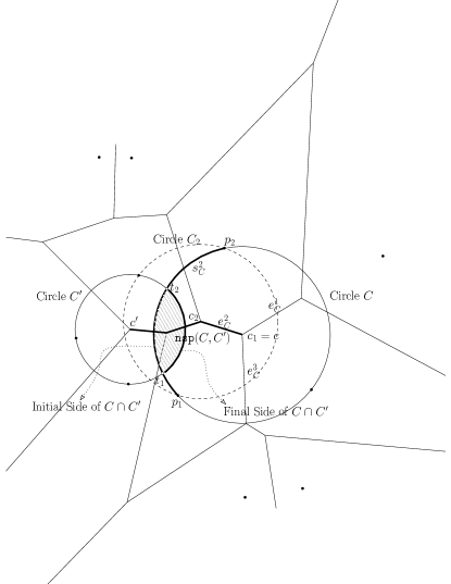
Figure 7: Illustration of $\Pi(c,c^{\prime})$.

Let $\mathbf{\Pi}(c,c^{\prime})$ as constructed above be $(c_{1}=c,c_{2},\ldots,c_{i},c_{i+1},\ldots,c^{\prime})$. Let $C_{2}$ denote the MEC centered at $c_{2}$. If $C_{2}$ is the circle $C^{\prime}$, then the procedure terminates and, as required, every MEC in the edge $(c,c_{2})$ encloses $C\cap C_{2}=C\cap C^{\prime}$.

Therefore, consider the case where $C_{2}$ is not $C^{\prime}$. Let $p_{1},p_{2}\in P$ be the points at which $C$ and $C_{2}$ intersect; $p_{1},p_{2}$ are the end points of the arc $s^{j}_{C}$ that defines the next step move toward $c^{\prime}$ (in Figure 7, $j$ is $2$). Therefore, by definition, $t_{1}$ and $t_{2}$ lie on the arc $s^{j}_{C}$. Notice that $C\cap C^{\prime}$ (shown shaded in Figure 7) is shaped like a rugby ball with $t_{1}$ and $t_{2}$ at its end-points. One side of $C\cap C^{\prime}$ (called the initial side) is in $C$ and the other side (called the final side) is in $C^{\prime}$. Clearly, $t_{1}$ and $t_{2}$ are inside (or on the boundary of) every MEC centered on the edge $e^{j}_{C}$. Otherwise, as we go from $C$ to $C_{2}$, there will be a circle that touches the final side of $C\cap C^{\prime}$, but that would mean that we have either

• reached $C^{\prime}$, which contradicts our assumption that $C_{2}$ is not $C^{\prime}$,

• or found a MEC that contains $C^{\prime}$, which contradicts the fact that $C^{\prime}$ is itself an MEC.

We now make two observations: (i) $C$ touches the initial side, but (ii) no other MECs centered on $e^{j}_{C}$ (and $C_{2}$ in particular) touches the final side Suppose (for the sake of contradiction) that there is a MEC $C^{*}$ centered on $e^{j}_{C}$ that touches the final side of $C\cap C^{\prime}$ at, say, some point $t^{*}$. It is easy to see that $C^{*}$ will contain $C^{\prime}$ because it touches $t^{*}$ on $C^{\prime}$ and contains $t_{1}$ and $t_{2}$, which are also on $C^{\prime}$ — this is a contradiction due to the observations (i) and (ii), stated above. Thus, it is clear that $C\cap C^{\prime}$ is properly contained within $C\cap C_{2}$.

Consider two adjacent vertices $c_{i}$ and $c_{i+1}$ along $\Pi(c,c^{\prime})$ with MECs $C_{i}$ and $C_{i+1}$ centered on them, respectively. The above argument can be easily extended to give us the following:

$$C_{i}\cap C^{\prime}\subset C_{i+1}\cap C^{\prime}.$$

Therefore, we can conclude that every MEC along $\Pi(c,c^{\prime})$ encloses $C\cap C^{\prime}$. Given Lemma 11, we can also conclude that $\Pi(c,c^{\prime})$ does not form a cycle. The only stopping condition is when we actually reach $c^{\prime}$, so $\Pi(c,c^{\prime})$ terminates at $c^{\prime}$ in $O(n)$ steps. Therefore, $\Pi(c,c^{\prime})$ fulfils our requirements.

To complete the proof of this lemma, we must show that $\Pi(c,c^{\prime})$ is the only required path. For the sake of contradiction, assume that there is another path $\Pi^{\prime}$ such that every MEC centered on $\Pi^{\prime}$ contains $C\cap C^{\prime}$. Then, there are two distinct paths from $c$ to $c^{\prime}$ such that every MEC centered on both paths overlapped with $C\cap C^{\prime}$. Clearly, there must be a cycle when the two paths are combined. From Lemma 11, we know that there are pairs of MECs in the cycle that will not overlap each other. This is a contradiction, thus proving that $\Pi(c_{1},c_{2})$ is the only required path and concluding the proof of the lemma. ∎

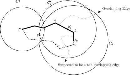
Figure 8: Illustrates the usefulness of the Unique Path Lemma.

To illustrate the usefulness of the unique path lemma, consider the example depicted in Figure 8. Let $C^{q}$ (centered at $c^{q}$) be the MEC returned by the LCQ data structure when queried with $q$. Suppose that $C_{q}$ (centered on $c_{q}$) is the largest empty circle containing $q$. Suppose Procedure 2 reports $C^{\prime}_{q}$ centered on $c^{\prime}_{q}$, which lies on an overlapping edge $(a,b)$. In terms of size, let $C^{q}<C^{\prime}_{q}<C_{q}$. Such a behavior will render our algorithm incorrect. However, this incorrect behavior is only possible when $c_{q}$ does not lie on an overlapping edge with respect to $c^{q}$, and therefore, Procedure 2 may never find it. This may happen in two possible situations:

Situation 1:

The path shown in thick continuous segments is $\Pi(c^{q},c_{q})$. Since Procedure 2 reported $c_{q}^{\prime}$, the edge $(a,b)$ is an overlapping edge, the MEC at $b$ must be larger than $C^{q}$. However, the LCQ data structure did not report the MEC at $b$, but rather reported $C^{q}$. While $q\in C^{q}$ and $q\in C_{q}$, $q$ is not contained within the MEC at $b$. From the unique path lemma, clearly, $b$ cannot be in $\Pi(c^{q},c_{q})$. Thus such a situation is impossible.

Situation 2:

Some other path that does not contain $c_{q}^{\prime}$ (shown using dashed line segments) is $\Pi(c^{q},c_{q})$. This case is possible and the edge $(c,b)$, shown in Figure 8, is an overlapping edge through that dashed path. Therefore, the edge $(c,b)$ will be considered by Procedure 2 and $C_{q}$ will be reported correctly.

Lemma 13

If a set $P$ of points from $\mathbb{R}^{2}$ are preprocessed by Procedure 1, then Procedure 2, when invoked with a query point $q$, correctly reports the largest circle that contains $q$ but is devoid of points from $P$.

Proof

Let $C_{q}$ be the largest circle that contains $q$ but is devoid of points from $P$. In short, Procedure 2 must report $C_{q}$. If $C_{q}$ is centered on a Voronoi vertex, then, clearly, Procedure 2 reports it correctly.

We now show that if $q$ is contained by a MEC centered at an artificial vertex $v$, then also the algorithm reports the correct $C_{q}$. Let $e$ be the half line edge containing $v$. Procedure 2 only searches edge $e$, which, we claim is sufficient. Suppose for the sake of contradiction that $C_{q}$ is centered on some other edge $e^{\prime}$. Clearly, $e^{\prime}$ cannot be a bounded Voronoi edge, because the MEC at $v$ is larger than MECs centered on bounded Voronoi edges. Recall that our construction of artificial vertices ensures that no two MECs centered on artificial vertices will overlap inside the convex hull of $P$. Therefore, $e^{\prime}$ cannot be an edge that is a half line either, because, the MEC at $v$ contains $q$, so the MEC centered at the artificial vertex on $e^{\prime}$ cannot contain $q$. Therefore, such an $e^{\prime}$ cannot exist and we can conclude that the algorithm correctly reports the largest MEC centered on some point in $e$ that contains $q$ as $C_{q}$.

For the rest of the proof, we assume that $C_{q}$ is not centered on a Voronoi vertex and $q$ is not enclosed by any MEC centered at an artificial vertex. Recall from Procedure 2 that $C^{q}$ is the largest MEC that is centered on a vertex and contains $q$. Clearly, $C^{q}\cap C_{q}\neq\emptyset$ as it at least contains $q$. From Lemma 12, there is exactly one path $\Pi(c^{q},c_{q})$ from the center of $C^{q}$ to the center of $C_{q}$ such that every circle in that path contains $C^{q}\cap C_{q}$. Clearly, MECs centered at vertices in $\Pi(c^{q},c_{q})$ other than the centers of $C^{q}$ and $C_{q}$ are smaller than $C^{q}$; otherwise, the LCQ data structure would not have chosen $C^{q}$. However, $C_{q}$ is larger than $C^{q}$. Consider the two vertices connected by the edge that contains the center of $C_{q}$. The MEC centered on one of them must be strictly larger than $C^{q}$, while the MEC on the other must be strictly smaller than $C^{q}$. Therefore, it is easy to see that $C_{q}$ is centered on an overlapping edge. Since the algorithm searches through all overlapping edges, it will find and report $C_{q}$ correctly. ∎

Lemma 10 coupled with the line sweep method of implementing the LCQ data structure and Lemma 13 immediately lead to the following theorem.

Theorem 5.1

Given a set $P$ of points in $\mathbb{R}^{2}$, we can preprocess $P$ in $O(n^{2}\log n)$ time and $O(n^{2})$ space so that the resulting data structure can be queried for the largest empty circle containing the query point $q$ in $O(\log n)$ time.

6 QMER problem

The input consists of a set of points $P=\{p_{1},p_{2},\ldots,p_{n}\}$ in a rectangular region $\cal A$. An axis-parallel rectangle inside $\cal A$ is said to be an empty rectangle if it does not contain any point of $P$. An empty rectangle is called maximal empty rectangle (MER) if no other empty rectangle in $\cal A$ properly contains it. Here our objective is to preprocess $P$ such that given any arbitrary query point $q\in\cal A$, the largest area rectangle $L(q)$ inside $\cal A$ that does not contain any point in $P$ but contains $q$, can be reported efficiently. First observe that $L(q)$ is an MER. Let $M$ denote the set of all possible MERs in $\cal A$. In [20], it is shown that $|M|=\Theta(n^{2})$ in the worst case.

In the preprocessing phase, we partition $\cal A$ into a set $C$ of cells, such that for every point $q$ inside a cell $c\in C$, the largest MER containing $q$ is the same. This is achieved by drawing horizontal and a vertical lines through each point in $P$. This splits $\cal A$ into the set $C$ of $O(n^{2})$ cells. Observe that for any cell $c\in C$ and any MER $M_{\alpha}\in M$, either $c\cap M_{\alpha}=c$ or $c\cap M_{\alpha}=\phi$. Therefore, if the query point $q$ lies inside $c\in C$, we need to report the largest MER containing $c$. We choose a representative point inside each cell $c\in C$. Let $Q$ be the set of representative points. We compute all the MERs using the algorithm in [20], and sort them with respect to their area. We also construct an augmented dynamic range tree ${{\cal{T}}}$ with the points in $Q$ in $O(n^{2}\log n)$ time and space [19]. Next, we process the members in $M$ in order. For each $M_{\alpha}\in M$, we identify the set $Q_{\alpha}$ of points in $Q$ that are inside $M_{\alpha}$. We store a pointer to $M_{\alpha}$ along with each point in $Q_{\alpha}$ and then delete $Q_{\alpha}$ from ${{\cal{T}}}$. This step takes $O(L+\log n)$ time [19], where $L$ is the number of points inside $M_{\alpha}$. After processing all the MERs in $M$, we have stored a pointer to the largest MER along with each $q\in Q$. Thus, we have the following theorem:

Theorem 6.1

A set of $n$ points in a rectangle $A$ can be preprocessed in $O(n^{2}\log n)$ time and space so that the largest empty rectangle query containing the query point can be answered in $O(\log n)$ time.

Moreover, it is not hard to see that we can construct examples, where there are $\Omega(n^{2})$ cells, so that the MER containing each of these cells is combinatorially different, i.e., the boundary of any of the two MERs are not incident to the same set of points in $P$. This suggests that in order to answer queries in polylogarithmic time, we need to somehow store $\Omega(n^{2})$ cells in a data structure, and hence it is very unlikely to improve the cost of preprocessing in order to maintain $O(\log n)$ query time.

7 Future Work

Our focus in this paper has been in terms of understanding which problems can be solved within subquadratic preprocessing time, while maintaining the polylogarithmic query time. At this stage the central problem here is to understand whether the preprocessing time for the QMEC problem for the point set case can be tightened to a subquadratic bound. A possible lead for improvement is as follows. If we were to insert $q$ into the set of points $P$, and compute the Delaunay triangulation of the new set, then the query circle, $C_{q}$, is a circumcircle of one of the triangles $t$ incident to $q$ - in fact the angle subtended at $q$ in $t$ will be greater than $\pi/2$. The running time for inserting $q$ in the Delaunay triangulation of $P$ is proportional to the degree of $q$. One may be tempted to use a (randomized) incremental algorithm for constructing Delaunay triangulation, but there are cases in which the degree of $q$ can be linear. This approach may lead to a practical and a simpler way to handle these types of queries, but this remains to be seen. Alternatively, one may look into the divide and conquer algorithms for computing the Voronoi diagram, and see whether in the “merge step”, the maximal empty circles can be maintained. Alternatively, one may try to use the planar separator theorem to partition the Voronoi diagram, recursively, and for the separator vertices (point), build an appropriate structure, so that preprocessing can be performed in subquadratic time, and the queries can be answered in sublinear time.

It will be desirable to improve the preprocessing cost in the case of simple polygons. A real challenge will be to match the complexity in this case to exactly that of the convex polygon case.

While we have studied a few canonical problems, there are several other variants that are as yet untouched. We can also ask similar questions on multidimensional geometric sets, but we suspect that the curse of dimensionality might restrict us to approximations.

Acknowledgments: We are grateful to Samir Datta and Vijay Natarajan for their helpful suggestions and ideas. We are also thankful to Subir Ghosh for providing the environment to carry out this work.

References

- [1] A. Aggarwal, L. J. Guibas, J. Saxe and P. W. Shor, A linear time algorithm for computing the Voronoi diagram of a convex polygon, Proc. of the 19th Annual ACM Symposium on Theory of Computing, pp. 39-45, 1987.
- [2] A. Aggarwal, S. Suri, Fast algorithms for computing the largest empty rectangle, Proc. of the 3rd Annual Symposium on Computational Geometry, pp. 278 - 290, 1987.
- [3] B. Aronov and M. Sharir, Cutting circles into pseudo-segments and improved bounds for incidences, Discrete Computational Geometry, vol. 28, pp. 475-490, 2000.
- [4] J. Augustine, B. Putnam, and S. Roy, Largest empty circle centered on a query line, Journal of Discrete Algorithms, vol. 8, pp. 143-153, 2010.
- [5] R. P. Boland and J. Urrutia, Finding the largest axis aligned rectangle in a polygon in time, Proc. of the Canad. Conf. on Computational Geometry, pp. 41-44, 2001.
- [6] M. A. Bender, and M. Farach-Colton, The level ancestor problem simplified, Theoretical Computer Science, vol. 321, pp. 5-12, 2004.
- [7] B. Chazelle, and R. Cole, and F. P. Preparata, and C. Yap, New upper bounds for neighbor searching, Information and Control, vol. 68, pp. 105-124, 1986.
- [8] B. Chazelle, R. L. Drysdale III and D. T. Lee, Computing the largest empty rectangle, SIAM J. on Computing, vol. 14, pp. 134-147, 1985.
- [9] J. Chaudhuri, S. C. Nandy, S. Das, Largest empty rectangle among a point set, Journal of Algorithms, vol. 46, pp. 54-78, 2003.
- [10] F. Y. L. Chin, J. Snoeyink, and C. A. Wang, Finding the medial axis of a simple polygon in linear time, Discrete Computational Geometry, vol. 21, pp. 405-420, 1999.
- [11] K. L. Daniels, V. J. Milenkovic, D. Roth, Finding the largest area axis-parallel rectangle in a polygon, Computational Geometry, vol. 7, pp. 125-148, 1997.
- [12] D. Dobkin and S. Suri, Dynamically computing the maxima of decomposable functions with applications, Proc. of the 30th Annual Symposium on Foundations of Computer Science, pp. 488-493, 1989.
- [13] J. R. Driscoll, N. Sarnak, D. D. Sleator, and R. E. Tarjan, Making data structures persistent, Proc. of the 18th. Annual ACM Symposium on Theory of Computing, pp. 109-121, 1986.
- [14] W. L. Hsu and K. H. Tsai, Linear time algorithm on circular-arc-graphs, Information Processing Letters, vol. 40, pp. 123-129, 1991.
- [15] H. Imai, M. Iri and K. Murota, Voronoi diagram in the Laguerre geometry and its applications, SIAM Journal on Computing, vol. 14: 93-105, 1985.
- [16] C. Jordan, Sur les assemblages de lignes, Journal fur die Reine und Angewandte Mathematik vol. 70, pp. 185-190, 1869.
- [17] R. Janardan and F. P. Preparata, Widest empty corridor problem, Nordic Journal on Computing, vol. 1, pp. 1-2, 1234.
- [18] D. G. Kirkpatrick, Optimal search in planar subdivisions, SIAM Journal on Computing, vol. 12, pp. 28-35, 1983.
- [19] K. Mehlhorn and S. Naher, Dynamic fractional cascading, Algorithmica, vol. 5, pp. 215-241, 1990.
- [20] A. Naamad, W.-L. Hsu and D. T. Lee, On the maximum empty rectangle problem, Discrete Applied Mathematics, vol. 8, pp. 267-277, 1984.
- [21] S. C. Nandy, A. Sinha, B. B. Bhattacharya, Location of the largest empty rectangle among arbitrary obstacles, Proc. of the 14th Annual Conf. on Foundations of Software Technology and Theoretical Computer Science, LNCS-880, pp. 159-170, 1994.
- [22] M. Orlowski, A new algorithm for the largest empty rectangle problem, Algorithmica, vol. 5, pp. 65-73, 1990.
- [23] F. P. Preparata and M. I. Shamos, Computational Geometry: An Introduction, Springer, 1975.
- [24] N. Sarnak and R. E. Tarjan, Planar point location using persistent search trees, Communications of the ACM vol. 29, pp. 669-679, 7 July 1986.
- [25] G. Toussaint, Computing largest empty circles with location constraints, International Journal of Parallel Programming, vol. 12, pp. 347-358, 1983.
- [26] H. Tamaki and T. Tokuyama, How to cut pseudo-parabolas into segments, Discrete Computational Geometry, vol. 19, pp. 265-290, 1998.