Conjectured Exact Percolation Thresholds of the Fortuin-Kasteleyn Cluster for the $\pm J$ Ising Spin Glass Model

Abstract

The conjectured exact percolation thresholds of the Fortuin-Kasteleyn cluster for the $\pm J$ Ising spin glass model are theoretically shown based on a conjecture. It is pointed out that the percolation transition of the Fortuin-Kasteleyn cluster for the spin glass model is related to a dynamical transition for the freezing of spins. The present results are obtained as locations of points on the so-called Nishimori line, which is a special line in the phase diagram. We obtain $T_{FK}=2/\ln[z/(z-2)]$ and $p_{{}_{FK}}=z/[2(z-1)]$ for the Bethe lattice, $T_{FK}\to\infty$ and $p_{{}_{FK}}\to 1/2$ for the infinite-range model, $T_{FK}=2/\ln 3$ and $p_{{}_{FK}}=3/4$ for the square lattice, $T_{FK}\sim 3.9347$ and $p_{{}_{FK}}\sim 0.62441$ for the simple cubic lattice, $T_{FK}\sim 6.191$ and $p_{{}_{FK}}\sim 0.5801$ for the 4-dimensional hypercubic lattice, and $T_{FK}=2/\ln\{[1+2\sin(\pi/18)]/[1-2\sin(\pi/18)]\}$ and $p_{{}_{FK}}=[1+2\sin(\pi/18)]/2$ for the triangular lattice, when $J/k_{B}=1$, where $z$ is the coordination number, $J$ is the strength of the exchange interaction between spins, $k_{B}$ is the Boltzmann constant, $T_{FK}$ is the temperature at the percolation transition point, and $p_{{}_{FK}}$ is the probability, that the interaction is ferromagnetic, at the percolation transition point.

1 Introduction

To establish reliable analytical theories of spin glasses has been one of the most challenging problems in statistical physics for years[1, 2, 3, 4, 5, 7, 6]. Our main interest in this article does not lie directly in the issue of the properties of the phases in spin glasses. We instead will concentrate ourselves on the precise determination of the structure of phase diagram for spin glasses. This problem is of practical importance for numerical studies, since exact locations of transition points greatly facilitate reliable estimates of physical properties around the transition points.

The $\pm J$ model is known as one of the Ising spin glass models[1, 2, 3, 4, 5, 6]. In this article, the percolation transition of the Fortuin-Kasteleyn (FK) cluster is investigated. The FK cluster has the FK representation[13, 14]. In the ferromagnetic Ising model, the percolation transition point agrees with the phase transition point[15]. The $\pm J$ model has a conflict in the interactions: the percolation transition point disagrees with the phase transition point. However, it was pointed out by de Arcangelis et al.[8] that the correct understanding of the percolation phenomenon of the FK cluster in the Ising spin glass model is important since a dynamical transition occurs at a temperature very close to the percolation temperature, and the dynamical transition and percolation transition are related to a transition for a signal propagating between spins. The dynamical transition is a transition for the freezing of spins, which is investigated by a distance called the damage or the Hamming distance[8, 9, 10, 11].

A line in the phase diagram for the $\pm J$ model is called the Nishimori line[3]. The internal energy, the upper bound of the specific heat and so forth are exactly calculated on the line[1, 2, 3, 4, 5, 6]. In addition, the internal energy does not depend on any lattice shape and instead depends on the number of nearest-neighbor pairs in the whole system. The location of the multicritical point can be on the Nishimori line, is conjectured on the square lattice, and the conjectured location is in good agreement with the results of other numerical estimates[12]. The present results are also obtained as locations of points on the Nishimori line.

We use a conjecture and the values of the threshold fractions of the random bond percolation problem for obtaining results in this article. If a threshold fraction of the random bond percolation problem is calculated, one is able to calculate the conjectured percolation threshold of the FK cluster in the $\pm J$ model by using the present theory. Generally, calculation of the threshold fractions of the random bond percolation problem is easier than that of the percolation thresholds of the FK cluster in the $\pm J$ model. Therefore, the present theory can be promising in this respect.

This article is organized as follows. In §2, the $\pm J$ model is explained. In §3, our conjecture is described, and conjectured exact equations are shown. The present results by using the obtained equations are given in §4. In §5, the concluding remarks of this article are described.

2 Model

The Hamiltonian for the $\pm J$ model, ${\cal H}$, is given by[1, 7]

$${\cal H}=-\sum_{\langle i,j\rangle}J_{i,j}S_{i}S_{j}\,,$$ (1)

where $\langle i,j\rangle$ denotes nearest-neighbor pairs, $S_{i}$ is a state of the spin at site $i$, and $S_{i}=\pm 1$. $J_{i,j}$ is the strength of the exchange interaction between the spins at sites $i$ and $j$. The value of $J_{i,j}$ is given with a distribution $P(J_{i,j})$. The distribution $P(J_{i,j})$ is given by

$$P(J_{i,j})=p\,\delta_{J_{i,j},J}+(1-p)\,\delta_{J_{i,j},-J}\,,$$ (2)

where $J>0$, and $\delta$ is the Kronecker delta. $p$ is the probability that the interaction is ferromagnetic, and $1-p$ is the probability that the interaction is antiferromagnetic.

We apply a percolation theory. We use the Fortuin-Kasteleyn (FK) cluster[13, 14]. The FK clusters consist of the FK bonds which are probabilistically put between spins. The number of the FK bonds is rigorously related to the internal energy[6]. We define the probability for putting the FK bond as $P_{FK}$. $P_{FK}$ is given by[8, 16]

$$P_{FK}=1-e^{-\beta J_{ij}S_{i}S_{j}-\beta|J_{ij}|}\,,$$ (3)

where $\beta=1/k_{B}T$, $T$ is the temperature, and $k_{B}$ is the Boltzmann constant. For calculating $[\langle P_{FK}\rangle_{T}]_{R}$, a gauge transformation is used, where $\langle\,\rangle_{T}$ denotes the thermal average. The gauge transformation is performed by[1, 17]

$$J_{i,j}\to J_{i,j}\sigma_{i}\sigma_{j}\,,\quad S_{i}\to S_{i}\sigma_{i}\,,$$ (4)

where $\sigma_{i}$ is a variable at site $i$, and $\sigma_{i}=\pm 1$. The gauge transformation has no effect on thermodynamic quantities[17]. By performing the gauge transformation, the ${\cal H}$ part becomes ${\cal H}\to{\cal H}$ and the $P_{FK}$ part becomes $P_{FK}\to P_{FK}$. By using Eq. (2), the distribution $P(J_{i,j})$ is rewritten as[1]

$$P(J_{i,j})=\frac{e^{\beta_{P}J_{i,j}}}{2\cosh(\beta_{P}J)}\,,\quad J_{i,j}=\pm J\,,$$ (5)

where $\beta_{P}$ is given by

$$\beta_{P}=\frac{1}{2J}\ln\frac{p}{1-p}\,.$$ (6)

By performing the gauge transformation, the distribution $P(J_{i,j})$ part becomes

$$\prod_{\langle i,j\rangle}P(J_{i,j}) = \frac{e^{\beta_{P}\sum_{\langle i,j\rangle}J_{i,j}}}{[2\cosh(\beta_{P}J)]^{N_{B}}}$$ (7)

$$\to \frac{\sum_{\{\sigma_{i}\}}e^{\beta_{P}\sum_{\langle i,j\rangle}J_{i,j}\sigma_{i}\sigma_{j}}}{2^{N}[2\cosh(\beta_{P}J)]^{N_{B}}}\,,$$

where $N_{B}$ is the number of nearest-neighbor pairs in the whole system. When the value of $\beta_{P}$ is consistent with the value of the inverse temperature $\beta$, the line for $\beta=\beta_{P}$ in the phase diagram is called the Nishimori line[3]. By using the gauge transformation, $[\langle P_{FK}\rangle_{T}]_{R}$ on the Nishimori line is obtained as[6, 16]

$$[\langle P_{FK}\rangle_{T}]_{R}=\tanh(\beta_{P}J)\,,$$ (8)

where $\beta_{P}=1/k_{B}T_{P}$, and $T_{P}$ is the temperature on the Nishimori line. The value of $[\langle P_{FK}\rangle_{T}]_{R}$ on the Nishimori line does not depend on any lattice shape.

The dynamical transition mentioned in this article is characterized by a distance between two spin configurations $\{S_{i}\}$ and $\{\tilde{S}_{i}\}$. By using the distance, the freezing of spins is investigated. The distance $D(t)$ is given by[10, 11]

$$D(t)=\frac{1}{2N}[\langle\sum_{i}^{N}|S_{i}(t)-\tilde{S}_{i}(t)|\rangle_{\rm MC}]_{R}\,,$$ (9)

where $t$ is the time, $N$ is the number of sites, $\langle\,\rangle_{\rm MC}$ denotes the sample average by the Monte Carlo method, and $[\,]_{R}$ denotes the random configuration average for the exchange interactions. As for the initial condition of $\{S_{i}\}$ and $\{\tilde{S}_{i}\}$, $\{S_{i}(0)\}$ is set to random, and $\{\tilde{S}_{i}(0)\}=-\{S_{i}(0)\}$ is set, for example. As for the initial condition, the two configurations are generally set to have a relationship with each other. As for the Monte Carlo method, a heat-bath method is used: by using the uniform pseudo-random number $r(t)$ $(0\leq r(t)<1)$, update of $\{S_{i}(t)\}$ and $\{\tilde{S}_{i}(t)\}$ is given by

$$S_{i}(t+\Delta t) = {\rm sign}\biggl{\{}\frac{1}{1+\exp[-2\beta\sum_{j}J_{i,j}S_{j}(t)]}-r(t)\biggr{\}}\,,$$ (10)

$$\tilde{S}_{i}(t+\Delta t) = {\rm sign}\biggl{\{}\frac{1}{1+\exp[-2\beta\sum_{j}J_{i,j}\tilde{S}_{j}(t)]}-r(t)\biggr{\}}\,,$$ (11)

where $\Delta t$ is a time step per spin, the summations of the right-hand sides of Eqs. (10) and (11) are over the nearest-neighbor sites of the site $i$. The two spin configurations $\{S_{i}(t)\}$ and $\{\tilde{S}_{i}(t)\}$ are updated with the same pseudo-random number sequence $\{r(t)\}$. It has been pointed out that, for the cubic lattice, there are three phases[10], i.e., a high-temperature phase, an intermediate phase and a low-temperature phase. In the high-temperature phase, the two configurations become identical quickly, so that the distance between them vanishes. In the intermediate phase and the low-temperature phase, the distance between the two configurations remains a finite in the long-time limit if the system size is large enough. In the intermediate phase, the distance between the two configurations does not depend on the initial conditions of the two configurations. In the low-temperature phase, the distance between the two configurations depends on the initial conditions of the two configurations. It is pointed out that the dynamical transition temperature $T_{D}$ between the high-temperature phase and the intermediate phase is related to the percolation transition temperature $T_{FK}$ of the FK cluster[8, 9]. It is pointed out in Refs.[8, 9] that there is a possibility that the value of $T_{FK}$ is consistent with the value of $T_{D}$. Recently, it was pointed out in Ref.[30] that, by a Monte Carlo calculation, the value of $T_{FK}$ is not consistent with the value of $T_{D}$, and the value of $T_{FK}$ is an approximated value of $T_{D}$.

3 Conjecture

We use a conjecture. If the conjecture is correct, the present theory gives the exact values. Here, we describe the conjecture and show conjectured exact equations derived by using the conjecture.

We conjecture

$$[\langle P_{FK}\rangle_{T}]_{R}=P_{C}$$ (12)

at the percolation transition point of the FK cluster on the Nishimori line for arbitrary lattices, where $P_{FK}$ is the probability for putting the FK bond between spins, and $P_{C}$ is the threshold fraction of the random bond percolation problem. In the random bond percolation problem, bonds for generating clusters are randomly put on the edges of the lattice, and one of the clusters is percolated at the threshold fraction $P_{C}$ [18]. From Eq. (8), the value of $[\langle P_{FK}\rangle_{T}]_{R}$ on the Nishimori line does not depend on any lattice shape. From the fact, Eq. (12) is conjectured. We propose this conjecture in this article as a conjecture which may be exact.

By using Eqs. (6), (8) and (12), we obtain

$$T_{FK} = \frac{2J}{k_{B}\ln[(1+P_{C})/(1-P_{C})]}\,,$$ (13)

$$p_{{}_{FK}} = \frac{1}{2}(1+P_{C})\,.$$ (14)

Eqs. (13) and (14) are conjectured exact equations. By using Eqs. (13), (14) and the value of the threshold fraction $P_{C}$ of the random bond percolation problem, the values of the percolation transition temperature $T_{FK}$ and the percolation transition probability $p_{{}_{FK}}$ are calculated as the location of a point on the Nishimori line. The obtained values are conjectured exact values. Note that the percolation transition probability $p_{{}_{FK}}$ is the probability that the interaction is ferromagnetic at the percolation transition point.

Campbell and Bernardi have derived an equation for the energy $E$ in the $\pm J$ model and the threshold fraction $P_{C}$ of the random bond percolation problem, i.e., $E=JN_{B}\{1-2P_{C}/[1-\exp(-2\beta J)]\}$ on the assumption of a random active-bond spatial distribution[9]. By applying the energy and the temperature on the Nishimori line to this equation, the same equations (Eqs. (13) and (14)) are obtained[19], where the energy on the Nishimori line is $-N_{B}J\tanh(\beta_{P}J)$ [1].

In Ref.[16], the exact values of the percolation threshold of the FK cluster are also conjectured. The conjecture proposed in this article is more general, so that the present study includes finite-dimensional cases that are not mentioned in Ref.[16].

4 Results

We show the present results by applying the conjectured exact equations obtained in §3, i.e., Eqs. (13) and (14), to several lattices. The present results are obtained as locations of points on the Nishimori line.

For the Bethe lattice, the threshold fraction $P_{C}$ of the random bond percolation problem is obtained as $P_{C}=1/(z-1)$ [21], where $z$ is the coordination number. By using Eqs. (13) and (14), we obtain

$$T_{FK}=\frac{2J}{k_{B}\ln[z/(z-2)]}\,,\quad p_{{}_{FK}}=\frac{z}{2(z-1)}\,.$$

This is the result for the Bethe lattice. $T_{FK}$ agrees with the ferromagnetic transition temperature for the pure system, $T_{C}$ [22]. When $z=N-1$ and $J\to J/\sqrt{N}$, this model becomes the infinite-range model. Then, in the thermodynamic limit, we obtain $T_{FK}\to\infty$ and $p_{{}_{FK}}\to 1/2$ when $J/k_{B}=1$. This result for the infinite-range model agrees with $T_{FK}$ of the previous result in Ref.[20] and $T_{D}$ of the previous results in Refs.[11, 23].

For the square lattice, the threshold fraction of the random bond percolation problem is obtained as $1/2$ [18]. By using Eqs. (13) and (14), we obtain

$$T_{FK}=\frac{2}{\ln 3}\sim 1.820478\,,\quad p_{{}_{FK}}=\frac{3}{4}=0.75\,,$$

when $J/k_{B}=1$. This is the result for the square lattice. When $J/k_{B}=1$, the ferromagnetic transition temperature for the pure system, $T_{C}$, is $2/\ln(1+\sqrt{2})$ ($\sim 2.269$) [22] . $T_{FK}$ does not agree with $T_{C}$ in this case. The previous numerical results are $T_{FK}=1.81(2)$ and $1.82(3)$ [24] for $p=0.7$, $T_{FK}=1.83(2)$ and $1.83(3)$ [24] for $p=0.8$, $T_{D}\sim 1.8$ [11] for $p=1/2$, $T_{D}\sim 1.70$ [23] for $p=1/2$, and $T_{D}=1.69(2)$ [30] for $p=1/2$. This result agrees with the previous results for $T_{FK}$ in Ref.[24]. This result does not contradict with the previous result for $T_{D}$ in Ref.[11]. However, it seems that this result does not agree with the previous results for $T_{D}$ in Refs.[23, 30].

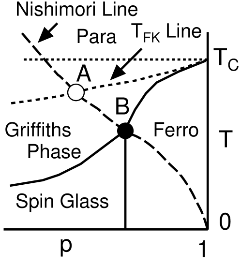
Figure 1: A schematic phase diagram for the $\pm J$ model. $p$ is the probability that the interaction is ferromagnetic, and $1-p$ is the probability that the interaction is antiferromagnetic. $T$ is the temperature. The paramagnetic phase (‘Para’), the ferromagnetic phase (‘Ferro’), the Griffiths phase (‘Griffiths Phase’) and the spin glass phase (‘Spin Glass’) are depicted. The Nishimori line (the dashed line), the Griffiths temperature (the dotted line) and the $T_{FK}$ line (the short dashed line) are also depicted. $T_{C}$ is the Curie temperature for the ferromagnetic model. The point ‘A’ is the percolation transition point of the FK cluster on the Nishimori line. The point ‘B’ is the multicritical point.

Fig.1 shows a schematic phase diagram for the $\pm J$ model. $p$ is the probability that the interaction is ferromagnetic, and $1-p$ is the probability that the interaction is antiferromagnetic. $T$ is the temperature. The paramagnetic phase (‘Para’), the ferromagnetic phase (‘Ferro’), the Griffiths phase (‘Griffiths Phase’) and the spin glass phase (‘Spin Glass’) are depicted. In this article, we do not mention the existence of a mixed phase between the ferromagnetic phase and the spin glass phase. The Nishimori line (the dashed line), the Griffiths temperature (the dotted line) and the $T_{FK}$ line (the short dashed line) are also depicted. $T_{C}$ is the Curie temperature for the ferromagnetic model. The value of the Griffiths temperature corresponds to the value of $T_{C}$. The $T_{FK}$ line represents the percolation transition temperature of the FK cluster. $T_{FK}$ agrees with $T_{C}$ [15] when $p=1$, and $T_{D}$ numerically agrees very well with $T_{C}$ [10] when $p=1$. The phase between the Griffiths temperature and the $T_{FK}$ line can also be called the Griffiths phase, but, it can be considered that the behavior of the distance in this phase is the same as that in the paramagnetic phase since $T_{FK}\sim T_{D}$. The point ‘A’ is the percolation transition point of the FK cluster on the Nishimori line. The point ‘B’ is the multicritical point. In a certain lattice case, $T_{FK}$ does not agree with $T_{C}$. On the other hand, in a certain lattice case, $T_{FK}$ agrees with $T_{C}$. For example, $T_{FK}$ for the square lattice does not agree with $T_{C}$ for the same lattice as mentioned above. On the other hand, $T_{FK}$ for the Bethe lattice agrees with $T_{C}$ for the same lattice as mentioned above. For the multicritical point, it seems that the temperature at the multicritical point generally does not agree with $T_{FK}$. For example, when $J/k_{B}=1$, the temperature at the multicritical point for the square lattice is roughly equal to $0.957$ [12], while $T_{FK}$ for the square lattice is $2/\ln 3$ ( $\sim 1.82$) from the present result. In addition, the temperature at the multicritical point for the Bethe lattice is $2J/k_{B}\ln[(\sqrt{z-1}+1)/(\sqrt{z-1}-1)]$ from the result in Ref.[25], while $T_{FK}$ for the Bethe lattice is $2J/k_{B}\ln[z/(z-2)]$ from the present result.

For the simple cubic lattice, the threshold fraction of the random bond percolation problem is numerically estimated as $P_{C}\sim 0.248813$ [26]. By using Eqs. (13) and (14), we obtain

$$T_{FK}\sim 3.9347\,,\quad p_{{}_{FK}}\sim 0.62441\,,$$

when $J/k_{B}=1$. This is the result for the simple cubic lattice. The previous numerical results are $T_{FK}\sim 3.92$ [8] for $p=1/2$, $T_{D}\sim 4.1$ [10] for $p=1/2$, $T_{D}\sim 4.0$ [11] for $p=1/2$, $T_{D}\sim 3.92$ [23] for $p=1/2$, and $T_{D}=3.932(2)$ [30] for $p=0.6244$. This result does not contradict with the previous results for $T_{FK}$ and $T_{D}$ in Refs.[8, 23]. This result slightly disagree with the previous result for $T_{D}$ in Ref.[30], but it seems that the difference between the two results is too small to judge the consistency. It seems that this result does not agree with the previous results for $T_{D}$ in Refs.[10, 11].

For the 4-dimensional hypercubic lattice, the threshold fraction of the random bond percolation problem is numerically estimated as $P_{C}\sim 0.16013$ [27]. By using Eqs. (13) and (14), we obtain

$$T_{FK}\sim 6.191\,,\quad p_{{}_{FK}}\sim 0.5801\,,$$

when $J/k_{B}=1$. This is the result for the 4-dimensional hypercubic lattice. The previous numerical results are $T_{D}\sim 6$ [11] for $p=1/2$, $T_{D}\sim 6.03$ [23] for $p=1/2$, and $T_{D}=6.057(10)$ [30] for $p=0.58006$. This result does not contradict with the previous results for $T_{D}$ in Refs.[11, 23], and this result slightly disagree with the previous result for $T_{D}$ in Ref.[30].

For the triangular lattice, the threshold fraction of the random bond percolation problem is obtained as $2\sin(\pi/18)$ [28]. By using Eqs. (13) and (14), we obtain

$$T_{FK}=\frac{2}{\ln\bigl{[}\frac{1+2\sin(\pi/18)}{1-2\sin(\pi/18)}\bigr{]}}\sim 2.759641\,,\quad p_{{}_{FK}}=\frac{1+2\sin(\pi/18)}{2}\sim 0.6736482\,,$$

when $J/k_{B}=1$. This is the result for the triangular lattice. The previous numerical results are $T_{FK}=2.74(3)$ and $2.73(4)$ [24] for $p=0.6$, and $T_{FK}=2.75(3)$ and $2.76(3)$ [24] for $p=0.7$. This result agrees with the previous results for $T_{FK}$ in Ref.[24].

The present result is possibly exact for $T_{FK}$.

5 Concluding Remarks

We theoretically showed the conjectured exact percolation thresholds of the FK cluster for the $\pm J$ Ising spin glass model based on a conjecture. The present theory possibly gives the exact values of the percolation transition temperature $T_{FK}$ on the Nishimori line. If the present theory is correct, one can obtain the possibly exact values [8, 9] or approximated values [30] of the dynamical transition temperature $T_{D}$ for the freezing of spins on the Nishimori line by using $T_{FK}\sim T_{D}$.

The present theory may be applied directly to the Gaussian Ising spin glass model and the Potts gauge glass model. Concretely, the solution of $[\langle P_{FK}\rangle_{T}]_{R}$ on the Nishimori line for the Gaussian Ising spin glass model is obtained in Ref.[16], and the solution of $[\langle P_{FK}\rangle_{T}]_{R}$ on the Nishimori line for the Potts gauge glass model is obtained in Ref.[29]. By using these solutions instead of the solution for the $\pm J$ Ising spin glass model, the conjectured exact equations in the Gaussian Ising spin glass model and the Potts gauge glass model are obtained.

Recently, it was numerically shown in Ref.[30] that $T_{FK}/T_{D}$ on the Nishimori line for the simple cubic lattice, a four-dimensional lattice and a five-dimensional lattice are $1.0005(5)$, $1.022(2)$ and $1.036(10)$ respectively. So, it was concluded that $T_{FK}$ does not equal to $T_{D}$ and the value of $T_{FK}$ is an approximated value of $T_{D}$.

We also mentioned the dynamical transition for the freezing of spins, which is investigated by the time evolution of the distance between two spin configurations on the Nishimori line. This study is different from the study of the aging phenomena on the Nishimori line as in Ref.[5].

References

- [1] H. Nishimori, J. of Phys. C 13 (1980) 4071; Prog. Theor. Phys. 66 (1981) 1169.
- [2] T. Morita and T. Horiguchi, Phys. Lett. A 76 (1980) 424.
- [3] H. Nishimori, Prog. Theor. Phys. 76 (1986) 305; J. Phys. Soc. Jpn. 55 (1986) 3305; J. Phys. Soc. Jpn. 61 (1992) 1011; J. Phys. Soc. Jpn. 62 (1993) 2793.
- [4] T. Horiguchi and T. Morita, J. of Phys. A 14 (1981) 2715.
- [5] Y. Ozeki, J. Phys. : Condens. Matter 9 (1997) 11171.
- [6] C. Yamaguchi, Prog. Theor. Phys. 127 (2012) 199.
- [7] S. F. Edwards and P. W. Anderson, J. Phys. F 5 (1975) 965.
- [8] L. de Arcangelis, A. Coniglio and F. Peruggi, Europhys. Lett. 14 (1991) 515.
- [9] I. A. Campbell and L. Bernardi, Phys. Rev. B 50 (1994) 12643.
- [10] B. Derrida and G. Weisbuch, Eurphys. Lett. 4 (1987) 657.
- [11] B. Derrida, Phys. Rep. 184 (1989) 207.
- [12] H. Nishimori and K. Nemoto, J. Phys. Soc. Jpn. 71 (2002) 1198.
- [13] P. W. Kasteleyn and C. M. Fortuin, J. Phys. Soc. Jpn. 26 (1969) Suppl. 11.
- [14] C. M. Fortuin and P. W. Kasteleyn, Physica (Utrecht) 57 (1972) 536.
- [15] A. Coniglio and W. Klein, J. of Phys. A 13 (1980) 2775.
- [16] C. Yamaguchi, Prog. Theor. Phys. 124 (2010) 399.
- [17] G. Toulouse, Commun. Phys. 2 (1977) 115.
- [18] S. Kirkpatrick, Rev. Mod. Phys. 45 (1973) 574.
- [19] C. Yamaguchi and I. A. Campbell, private communication.
- [20] J. Machta, C. M. Newman and D. L. Stein, J. Stat. Phys. 130 (2008) 113.
- [21] D. Stauffer and A. Aharony, Introduction to Percolation Theory, 2nd ed. (Taylor and Francis, London, 1992).
- [22] R. J. Baxter, Exactly Solved Models in Statistical Mechanics (Academic Press, London, 1982).
- [23] I. A. Campbell and L. de Arcangelis, Physica A 178 (1991) 29.
- [24] H. Imaoka, H. Ikeda and Y. Kasai, Physica A 246 (1997) 18.
- [25] J. M. Carlson, J. T. Chayes, L. Chayes, J. P. Sethna and D. J. Thouless, J. Stat. Phys. 61 (1990) 987.
- [26] C. D. Lorenz and R. M. Ziff, Phys. Rev. E 57 (1998) 230.
- [27] G. Paul, R. M. Ziff and H. E. Stanley, Phys. Rev. E 64 (2001) 026115.
- [28] M. F. Sykes and J. W. Essam, J. Math. Phys. 5 (1964) 1117.
- [29] C. Yamaguchi, arXiv:1001.1675.
- [30] P. H. Lundow and I. A. Campbell, arXiv:1204.6732.