Alternative Adaptive Filter Structures for improved radio frequency interference Cancellation in Radio Astronomy

Abstract

In radio astronomy, reference signals from auxiliary antennae, receiving only the radio frequency interference (RFI), can be modified to model the RFI environment at the astronomy receivers. The RFI can then be cancelled from the astronomy signal paths. However, astronomers typically only require signal statistics. If the RFI statistics are changing slowly, the cancellation can be applied to the signal correlations at a much lower rate than required for standard adaptive filters. In this paper we describe five canceller setups; pre- and post-correlation cancellers that use one or two reference signals in different ways. The theoretical residual RFI and added noise levels are examined, and demonstrated using microwave television RFI at the Australia Telescope Compact Array. The RFI is attenuated to below the system noise, a reduction of at least 20 dB. While dual-reference cancellers add more reference noise than single-reference cancellers, this noise is zero-mean and only adds to the system noise, decreasing the sensitivity. The residual RFI that remains in the output of single-reference cancellers (but not dual-reference cancellers) sets a non-zero noise floor that does not act like random system noise and may limit the achievable sensitivity. Thus dual-reference cancellers often result in superior cancellation. Dual-reference pre-correlation cancellers require a double-canceller setup to be useful and to give equivalent results to dual-reference post-correlation cancellers.

1. INTRODUCTION

Radio astronomy is poised to move ahead with a suite of new instruments such as the Square Kilometre Array (SKA). These instruments will improve sensitivity, resolution, bandwidth, and many other instrument and observational parameters by more than an order of magnitude. At present, many radio astronomy observations are corrupted to at least some extent by radio frequency interference (RFI). This interference comes from ground-based communication transmitters, satellites, and the observatory equipment itself. With the increase in sensitivity and frequency coverage of radio astronomy instruments, and with telecommunication signals occupying more of the spectrum, it is essential to develop ways of removing or suppressing this RFI.

In radio astronomy, real-time adaptive filters can be used to modify an auxiliary voltage time series (the reference signal) so that it cancels RFI from an astronomical voltage time series (Barnbaum & Bradley, 1998; Bower, 2001; Mitchell & Robertson, 2005). For each voltage sample the filters are allowed to slightly vary their internal coefficients in order to adapt to any changes taking place in the RFI. If one is interested in the power spectrum of the astronomy signal, and the filter coefficients stay fairly constant over the interval in which the power spectrum is estimated, cancellation in the post-correlation domain can give better results, since a second reference antenna can be used to give complete suppression of the RFI (only zero-mean random receiver noise is added to the complex correlations and it will average away, see Briggs et al. 2000; Mitchell & Bower 2001). However, many applications (particularly in the communications field, but also some astronomy applications), require the recovery of the actual symbol stream (i.e., a transmitted sequence of symbols such as bits or words) from the noisy RF environment, which is not retained in post-correlation. Following a suggestion of Briggs et al. (2000), we have devised a modified approach that can give improved RFI attenuation in the voltage domain. In an attempt to minimise any RFI in an astronomical voltage series the standard approach is to minimise the canceller’s output power, which it will be shown means that some residual RFI always remains. The modified approach that we give here forces the RFI in the output power to zero. It results in residual power that is always greater than that of the standard approach (output power is no longer minimised), but which does not contain RFI. That is, superior RFI cancellation is obtained, but at the expense of somewhat increased thermal noise.

In the following sections the standard adaptive canceller is discussed, and the new approach is introduced. This is followed by an overview of how cancellation can be applied after correlations are formed. Residual RFI power and added receiver noise are investigated and an example from the Australia Telescope Compact Array is given.

2. ADAPTIVE CANCELLERS

2.1. The Model

In an attempt to remain general, we assume a system of one or more radio antennae pointing towards a direction on the celestial sphere. Delays are inserted into the signal paths so that a wavefront from the chosen direction arrives at the output of each antenna simultaneously. The celestial location is known as the phase tracking centre (Thomson et al., 1986; Taylor et al., 1999). Given that we will attempt to deal with the interference in subsequent parts of the system, separate reference antennae are incorporated into the network of receivers to observe the RF environment, which typically enters the astronomy signal through the side-lobes of the antennae. Signals from astronomy antennae will be referred to as main signals, and those from reference antennae as reference signals. At each antenna a waveform containing an additive mixture of all the signals present in the environment is received and downconverted to an IF voltage series. This is sampled and quantised into a number of digital bits (which we assume is sufficient to keep the voltage statistics linear so that quantisation effects such as intermodulation are negligible, and to ensure that the receiver noise and astronomy fluctuations are measured even in the presence of strong interference). Each main IF voltage series contains three components: a noise voltage from the receiving system, $n(t)$; a noise voltage from the sky, $s(t)$; and interference, $i(t)$. The sky voltage contains the information about the astronomical sources, which are the signals of interest. If the interference cannot be removed completely, it is desirable to reduce it to less than the final RMS noise level (with a negligible – or at least predictable – effect on the astronomy, Barnbaum & Bradley 1998).

Since an interfering signal is usually incident from a direction other than the phase tracking centre, its wavefront will not be synchronous at the output of the different antennae. The geometric delay, $\tau_{k}$, of antenna $k$ – due to the physical separation of the receivers – represents the difference in arrival time of an interfering wavefront at antenna $k$ and an arbitrary reference point (after accounting for the delay needed to track the selected field on the celestial sphere).

As a signal passes through a receiving and processing system it encounters various convolutions and deconvolutions, so working in the frequency domain can offer a more intuitive basis for discussion. In the frequency domain the system can be represented by complex multiplications and divisions. A frequency-dependent coupling term, $G_{\nu}(t)$, is used to describe the combined complex-valued gain of each receiver system and antenna to the interference, including any filtering (time is included to account for the slow variations imposed as the RFI passes through antenna side-lobes). Using upper case characters to denote frequency domain quantities, and keeping in mind that this spectral representation comes from Fourier transforming each consecutive 1000 or so samples of the voltage series, the signal in a quasi-monochromatic channel at frequency $\nu$ is

$$V_{\nu,m}=N_{\nu,m}+G_{\nu,m}(t)I_{\nu}e^{j\phi_{\nu,m}(t)}+S_{\nu},\\$$ (1)

for main antennae and

$$V_{\nu,r}=N_{\nu,r}+G_{\nu,r}(t)I_{\nu}e^{j\phi_{\nu,r}(t)},\\$$ (2)

for reference antennae. Note that the phase term due to the geometric delay of the interfering signal, $\phi_{\nu,k}(t)=2\pi\nu\tau_{k}(t)$, has been kept separate from the $G$-terms (time is also included here to account for changes as either the phase tracking centre or RFI transmitter direction change). To remain general the $G$-terms are kept as complex quantities, to allow for any effects on the phase that are not due to the geometric delay. It is assumed that there is only one interfering signal in a frequency channel (see Bower 2001 for a discussion of multiple interferers), and that there is negligible reference antenna gain in the direction of $S$, i.e., reference antennae do not measure signal from astronomical sources. These are important assumptions, but often quite reasonable (the latter assumption is strengthened because the weak astronomy signal enters the reference antennae through side-lobes). However, statements made later in relation to the lack of effect of adaptive cancellers on the astronomy signal rely on the validity of the second assumption. If any astronomy signals leak into the reference series the achievable sensitivity, dynamic range, astronomy purity, etc., will all be affected. For example, signal leakage could lead to the power of a strong self-calibration source changing as the canceller weights change.

2.2. MK1: Single Reference Adaptive Cancellers

Adaptive cancellers are usually applied to broadband IF voltage samples in the time domain (Widrow & Stearns, 1985; Barnbaum & Bradley, 1998). (“Broadband” here simply refers to the whole passband, rather than the quasi-monochromatic frequency channels.) While the adaptive canceller examples given throughout section 4 have been processed in the time domain, the following analysis is carried out in the frequency domain (see Widrow & Stearns, 1985; Barnbaum & Bradley, 1998; and Bower, 2001 for descriptions of time domain implementation).

The aim of adaptive cancellers in interference mitigation is to find the set of filter weights, W, which scale and phase shift each reference antenna frequency channel so that they best approximate the RFI in a main astronomy spectrum (in the time domain delays are inserted into the signal paths so that positive and negative delays can be considered. So strictly speaking the cancellers are not truly real-time, the output is lagging in time by the length of the inserted delay.) So W is a vector with a complex element for each frequency channel. Figure 1 shows schematically how such a canceller can be implemented, hereinafter referred to as a mark one (MK1a) canceller (the “a” is added since we will be modifying the filter later).

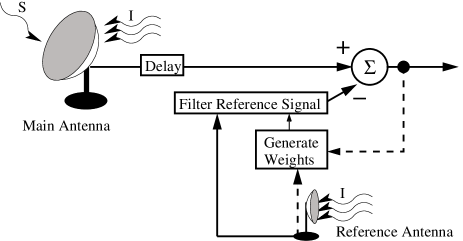
Figure 1.— Schematic of a MK1a adaptive canceller. Dashed lines indicate signal paths used to calculate the weights.

Throughout this paper it is assumed that the filter weights are varying slowly enough that they are approximately constant on the time scales used to calculate them; typically less than a second. It is also assumed that the various signals are independent (i.e., $S_{m}$, $I_{m}$, and $N_{m}$ are uncorrelated, and the receiver noise is independent for the different antennae, i.e., $N_{m}$ and $N_{r}$ are uncorrelated. The noise terms, $N$, will not be independent for receivers used in low frequency instruments such as LOFAR, where they will be dominated by partially correlated sky noise. Here we will only consider frequencies for which $N$ is dominated by uncorrelated noise, internal to the receivers.) When these assumptions hold, the power in a single frequency channel at the output of the canceller is

$$\begin{array}[]{rcl}P&=&\left<(V_{m}-WV_{r})(V_{m}-WV_{r})^{*}\right>\\ &&\\ &=&\left<|V_{m}|^{2}\right>-\left<V_{m}W^{*}V_{r}^{*}\right>-\\ &&\left<V_{m}^{*}WV_{r}\right>+\left<|WV_{r}|^{2}\right>,\end{array}$$ (3)

where * denotes a complex conjugate and $\left<...\right>$ the expectation value. The explicit frequency dependency of the terms has been removed (it is assumed that the channels are independent so that (3) can be applied to each frequency channel separately). If we set $\sigma_{I}^{2}=\left<|I|^{2}\right>$, $\sigma_{S}^{2}=\left<|S|^{2}\right>$, $\sigma_{N_{k}}^{2}=\left<|N_{k}|^{2}\right>$, and assume that the complex gains, delays, and weights are constant over the time average, so they can be taken outside the average, then we can write

$$\begin{array}[]{rcl}P&=&\sigma_{N_{m}}^{2}+\sigma_{S}^{2}+|G_{m}|^{2}\sigma_{I}^{2}-\\ &&W^{*}G_{m}G_{r}^{*}e^{j\phi_{mr}}\sigma_{I}^{2}-WG_{m}^{*}G_{r}e^{-j\phi_{mr}}\sigma_{I}^{2}+\\ &&|W|^{2}|G_{r}|^{2}\sigma_{I}^{2}+|W|^{2}\sigma_{N_{r}}^{2},\end{array}$$ (4)

where $\phi_{mr}$ represents the phase difference, $\phi_{m}-\phi_{r}$.

Equation (4) highlights a critical point. Minimising the output power reduces the combined power of the residual RFI and the inserted reference receiver noise. If there is reference receiver noise the RFI will never be completely cancelled (Widrow & Stearns, 1985; Barnbaum & Bradley, 1998). This is because both the interference and reference receiver noise are being weighted. The receiver noise of the main antennae and the astronomy signals, however, are not affected by the choice of weights and will pass through the canceller freely (under assumptions of signal independence and zero reference gain towards astronomy sources).

To perform the minimisation of $P$, one can differentiate it with respect to $W$ and find the weights that set the derivative equal to zero. The surface of $P$ is a multidimensional (positive) quadratic surface that has a single minimum, so the weights that set $dP/dW=0$ must give the unique global minimum (Widrow & Stearns, 1985; Barnbaum & Bradley, 1998). Alternatively, Wiener theory tells us that the optimal weights (known as the Wiener-Hopf solution), $W_{\it{mk1a}}$, which minimise the output power are also the weights that set the cross-correlation between the canceller output and the reference signal to zero (Widrow & Stearns 1985, as indicated in figure 1):

$$\left<(V_{m}-W_{\it{mk1a}}V_{r})V_{r}^{*}\right>=0,$$ (5)

$$\Rightarrow \displaystyle W_{\it{mk1a}}=\frac{\left<V_{m}V_{r}^{*}\right>}{\left<V_{r}V_{r}^{*}\right>}.$$ (6)

So the weighting process takes the cross-correlation of the reference and main signals, which determines the correlated power and relative delay of the interference, and scales that by the auto-correlation of the reference signal. One can calculate these weights directly by calculating the correlations from short integrations, or they can be found adaptively by iteratively seeking and then tracking the weights that satisfy (5).

Ideally the output of the canceller would consist of the astronomy signal and receiver noise. However, as mentioned above, since there is always some receiver noise in the reference signal, setting the correlation in (5) to zero can never remove all of the RFI. The RFI is played off against the reference receiver noise. If $\it{INR}_{r}$ is the interference-to-noise power ratio of the reference signal, $G_{r}^{2}\sigma_{I}^{2}/\sigma_{N_{r}}^{2}$, the mean amount of residual output power (power in addition to the main receiver noise and the astronomy, $R_{\it{mk1a}}=P_{\it{mk1a}}-\sigma_{N_{m}}^{2}-\sigma_{S}^{2}$), is given by

$$R_{\it{mk1a}}=\frac{G_{m}^{2}\sigma_{I}^{2}}{1+\it{INR}_{r}}.$$ (7)

It is clear from (7) that as $\it{INR}_{r}$ approaches infinity (no reference receiver noise) the residual power goes to zero. If there is no RFI, $G_{m}^{2}$ will be zero and there will also be zero residual power (the filter turns off). When $\it{INR}_{r}$ is finite and non-zero the reference receiver noise term in the denominator of (6) biases the weights and some residual power will remain. What might not be so clear from an inspection of (7) is the statement made earlier that this residual power is a combination of reference receiver thermal noise added during cancelling and residual RFI that was not excised. Another way to see this bias is to consider figure 1. Thermal noise from the reference receiver is present in both inputs to the weight generation process (in the $V_{r}$ term from the reference antenna and the $-W_{\it{mk1a}}V_{r}$ term from the filter output, c.f. equation 5). This will lead to a second non-zero-mean correlation product (the first being the RFI). Minimising the output power must be a trade-off between minimising the contributed reference receiver noise and the RFI, and as a result there will always be residual RFI. The total residual power given in (7) can be divided into the inserted reference receiver noise residual, $R_{\it{\it{mk1a}}}^{\it{(rx)}}$, and the RFI residual, $R_{\it{\it{mk1a}}}^{\it{(rfi)}}$, such that

$$R_{\it{\it{mk1a}}}=R_{\it{\it{mk1a}}}^{\it{(rfi)}}+R_{\it{\it{mk1a}}}^{\it{(rx)}},$$ (8)

which are shown by Mitchell 2004 to be

$$R_{\it{mk1a}}^{\it{(rfi)}}=\frac{G_{m}^{2}\sigma_{I}^{2}}{\it{INR}_{r}^{2}\left(1+\it{INR}_{r}^{-1}\right)^{2}},$$ (9)

$$R_{\it{mk1a}}^{\it{(rx)}}=\frac{G_{m}^{2}\sigma_{I}^{2}}{\it{INR}_{r}\left(1+\it{INR}_{r}^{-1}\right)^{2}}.$$ (10)

Thus $R_{\it{mk1a}}^{\it{(rfi)}}=R_{\it{mk1a}}^{\it{(rx)}}\,/\,\it{INR}_{r}$. To shed some light on the meaning of the relations in (9) and (10), we again interpret the process of output power minimisation as determining the weights that set the cross-correlation of the canceller output and the reference signal to zero. As $\it{INR}_{r}$ increases, the RFI becomes the dominant signal in the cross-correlation, and the filter must concentrate on reducing the RFI power. As a result the proportion of the RFI that remains after cancelling decreases faster than the injected noise power. When $\it{INR}_{r}<1$ noise starts to dominate and the filter will concentrate on reducing the contributed noise power. When $\it{INR}_{r}$ goes to zero, the correlation is completely reference receiver noise, and the canceller turns itself off. When RFI dominates, most of the residual power is reference receiver noise, and when reference receiver noise dominates, most of the residual power is RFI. Also, since the reference signal is being scaled in an attempt to match its own RFI to the RFI in the main signal, the larger $G_{r}$ is relative to $G_{m}$ (for example using a reference antenna that is pointing directly at the interfering source), the smaller the scaling factor (weighting amplitude) and thus the amount of injected receiver noise. When $\it{INR}_{r}\gg 1$ and $G_{r}\gg G_{m}$ both of the residual terms drop off and extremely good results are achieved (Barnbaum & Bradley, 1998; Bower, 2001).

2.3. MK2: Dual Reference Adaptive Cancellers

To remove the biasing effect caused by the reference receiver noise, a second reference receiver can be used, as was suggested in Briggs et al. (2000). The RFI in the main spectrum is still estimated using a weighted version of the spectral channels from the first reference, but now the cross-correlation of the second reference signal with the canceller output is set to zero in order to find the weights. This MK2a canceller is shown in figure 2.

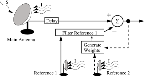
Figure 2.— Schematic of a MK2a adaptive canceller, which uses two reference signals. Dashed lines indicate signal paths used to calculate the weights.

It was mentioned in the previous section that the reference receiver noise is a component of both signals in (5). Zeroing this correlation results in minimum output power, but a non-zero RFI residual. Correlating the canceller output against a second reference with uncorrelated receiver noise removes the bias. Since the RFI is the only correlated signal, zeroing the cross-correlation results in zeroing the RFI. However, there is no built-in mechanism to guard against the amount of reference receiver noise contributed to the output. The amount added during cancelling must always be greater than the noise added by the MK1a canceller, since power is no longer minimised.

The two references will be denoted $r_{1}$ and $r_{2}$, so that

$$\begin{array}[]{rcl}V_{r_{1}}&=&N_{r_{1}}+G_{r_{1}}Ie^{j\phi_{r_{1}}}\mbox{, and}\\ \\ V_{r_{2}}&=&N_{r_{2}}+G_{r_{2}}Ie^{j\phi_{r_{2}}},\\ \end{array}$$ (11)

and we can again determine the weights that set the output-reference cross-correlation to zero:

$$\begin{array}[]{rl}&\left<(V_{m}-W_{\it{mk2a}}V_{r_{1}})V_{r_{2}}^{*}\right>=0\\ &\\ \Rightarrow&\displaystyle W_{\it{mk2a}}=\frac{\left<V_{m}V_{r_{2}}^{*}\right>}{\left<V_{r_{1}}V_{r_{2}}^{*}\right>}.\end{array}$$ (12)

As with the MK1a canceller the weights need to scale and phase shift reference signal $V_{r_{1}}$ so that its RFI component matches that of signal $V_{m}$. Here, however, the independent reference signal $r_{2}$ is used to give a true view of the scaling factor needed to match RFI levels. $W_{\it{mk2a}}$ is only constrained by the RFI, since the receiver noise terms in $\left<V_{r_{1}}V_{r_{2}}^{*}\right>$ are uncorrelated, and the RFI signal is entirely replaced with a weighted version of thermal noise from reference signal $V_{r_{1}}$ (assuming that the various signals are uncorrelated and that the receivers are ideal and remain linear). While the noise in the weights will also increase the output power of the canceller, it is much weaker noise since the weights are averaged over many samples, and is not considered further here. When $W_{mk2a}$ from (12) is substituted into the equation for output power, $P_{mk2a}=\left<|V_{m}-W_{mk2a}V_{r_{1}}|^{2}\right>$, the mean residual power is

$$R_{\it{mk2a}}=R_{\it{mk2a}}^{\it{(rx)}}=\frac{G_{m}^{2}\sigma_{I}^{2}}{\it{INR}_{r_{1}}},$$ (13)

as shown in Mitchell (2004). Infinite attenuation of the RFI component has been achieved, but potentially a significant amount of system noise has been added during cancelling. Compare (7) and (13): As in (7), when $\it{INR}_{r_{1}}\gg 1$, the attenuation of the RFI signal in $V_{m}$ is very large. In this case however, any frequency channels with $\it{INR}_{r_{1}}<1$ will end up with more unwanted power than they started with. The MK2a canceller does not turn itself off. The reference signal is boosted until its RFI matches the RFI in the main signal, regardless of the amount of receiver noise being added. Note that $\it{INR}_{r_{2}}$ does not affect the output power, provided there is enough RFI power in $V_{r_{2}}$ to keep the weights stable (see section 6 for a discussion of weight stability).

If one is interested in the (interference-free) power spectrum of $V_{m}$, the single reference antenna MK1a canceller output will contain less residual power. There are, however, advantages to the MK2a canceller. If one is concerned with retrieving a structured signal from a voltage series, random noise in the signal may not pose too much of a problem, but a structured RFI residual may detract from signal recovery. More relevant in radio astronomy is the case where one is looking for a structure in the power spectrum. The RFI remaining after MK1a cancelling will have features in the power spectrum, but if the (amplified and filtered) reference RFI, $G_{r_{1}}^{2}\sigma_{I}^{2}$, is proportional to $G_{m}^{2}\sigma_{I}^{2}$, equation (13) says that the noise contributed by MK2a cancelling will have the same spectrum as the input reference receiver noise (apart from a constant scaling factor). It is also conceivable to remove the unwanted reference receiver noise from the auto-correlation of either canceller’s output. This is discussed in the next section and can result in a MK2 canceller superior to the MK1 canceller for some applications.

2.4. Suppressing Added Reference Noise

We now describe a double canceller setup that can be used to suppress the added reference receiver noise in the output astronomy power spectrum. If the main signal is duplicated before cancelling so there is an identical copy, the copy can be passed through a second canceller that uses different reference signals so that the noise added will be uncorrelated with the noise added to the first. When the two filtered copies are cross-correlated, the main antenna receiver noise and astronomy will correlate as if the original signal has simply been auto-correlated, while the added reference noise power will average away with the radiometric factor ($\sqrt{\Delta\nu\tau_{\it{int}}}$).

An important point to note about the MK2a canceller is that all of the noise added during cancelling is from the first reference receiver (see equation 13). The second reference is only used in setting the complex weights. So the second canceller can be made by interchanging the references. This setup will be called the MK2b canceller and is shown in figure 3. As discussed in Mitchell (2004), if the INR of the references are the same, the mean residual output power from the MK2b canceller is

$$R_{\it{mk2b}}=\frac{R_{\it{mk2a}}}{\sqrt{\Delta\nu\tau_{\it{\it{int}}}}},$$ (14)

which averages towards zero as the integration length is increased.

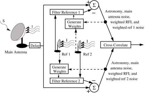
Figure 3.— MK2b canceller system where the auto-correlation is replaced by the cross-correlation of two independently processed copies of the main signal.

Similarly, if two references are used to create two independent MK1a cancellers for the two main signal copies, this gives the MK1b canceller shown in figure 4, and the mean residual output power becomes

$$R_{\it{mk1b}}=R_{\it{mk1a}}^{\it{(rfi)}}+\frac{R_{\it{mk1a}}^{\it{(rx)}}}{\sqrt{\Delta\nu\tau_{\it{int}}}}.$$ (15)

Figure 4.— MK1b canceller system where the auto-correlation is replaced by the cross-correlation of two independently processed copies of the main signal.

Equations (14) and (15) show that while $R_{\it{mk2b}}$ should keep integrating towards zero, $R_{\it{mk1b}}$ has a definite limit due to the RFI signal that remains after cancelling. However, one must be aware that in situations where the reference INR is very small the MK2 canceller does not turn itself off, and there are practical implementation issues that need to be addressed (essentially, one may need to force the canceller to turn off). This is discussed in section 6.

3. THEORETICAL RESULTS

In this section the residual power equations given throughout section 2 are demonstrated. Note that while the plots for the dual-reference cancellers show the residual power as the reference interference-to-noise power ratio approaches arbitrarily close to zero, the algorithms in practice become unstable and need to be turned off. This point will be reiterated where appropriate in the discussion below. For the theory we have set $\sigma_{S}^{2}=\sigma_{N_{m}}^{2}=0$, so that all of the output power displayed in this section is a combination of residual RFI and any reference receiver noise added during cancelling.

Figure 5 displays the proportion of residual power in the output signal after adaptive cancelling with MK1b and MK2b cancellers. The plot shows that the added reference receiver noise averages away as the integration length is increased. If single canceller systems were being considered, then since any noise added during cancelling is sent to an auto-correlator, the output power would remain constant (i.e., remain at the levels shown on the left hand side of figure 5). It is clear that the MK1b canceller hits a limit when it reaches the residual RFI, but that the MK2b does not.

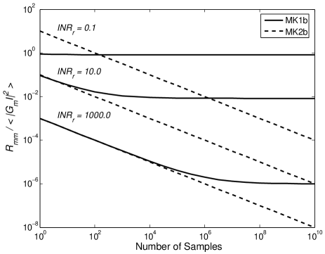
Figure 5.— Theoretical residual power (normalised by the main signal’s input RFI power) for various $\it{INR}_{r}$ values as a function of the number of samples used to average the noise down in the canceller output ($\Delta\nu\tau_{\it{int}}$). The three sets of solid and dashed lines are for $\it{INR}_{r}$ values of 0.1 (top), 10 (middle), and 1000 (bottom). Solid lines indicate MK1b cancelling, dashed lines MK2b cancelling. The lines flatten when the residual RFI power level is reached.

As $\it{INR}_{r}$ decreases the normalised output power of the MK1b canceller levels off at 1, so there is no cancelling taking place. On the other hand the MK2 canceller continues to insert more and more reference receiver noise in an attempt to match the reference RFI to the main signal RFI. Even though the MK2b canceller always has the larger total residual power, it is entirely zero-mean noise and averages out with the radiometric factor. Again the reader should note that for low $\it{INR}_{r}$ values the MK2 canceller can become unstable and requires an additional mechanism to turn off.

Figure 6 shows contours of constant (normalised) output power as a function of $\it{INR}_{r}$ and the number of samples, $\Delta\nu\tau_{\it{int}}$. Figures 6a and 6b represent MK1a and MK2a cancelling respectively, and figures 6c and 6d represent MK1b and MK2b cancelling respectively. The amount of residual power in dB is indicated by the grey scale and runs from -80 to 20 dB. It is clear from figure 6c that a constant RFI residual remains for all $\it{INR}_{r}$ values after MK1b cancelling. The dashed line indicates the approximate line where the added reference receiver noise power has averaged down to expose the non-zero residual RFI power level.

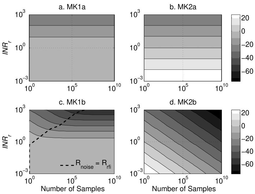
Figure 6.— Residual power contours as a function of $\it{INR}_{r}$ and $\Delta\nu\tau_{\it{int}}$. Greyscale indicates the normalised output power, $R_{mm}/(|G_{m}|^{2}\sigma_{I}^{2})$, expressed in dB. Figures a and b show MK1a and MK2a cancelling respectively. Figures c and d show MK1b and MK2b canceller output respectively.

It is clear from figures 6a and 6c that an output power plateau is reached as $\it{INR}_{r}$ becomes small for the MK1 cancellers. The residual power of the plateau is 0 dB, and indicates that the canceller has turned off. In contrast, the MK2a canceller (6b) does not turn off and results in more output power than input RFI power for low $\it{INR}_{r}$ levels. However, since the residual is entirely noise it averages down in a MK2b canceller, where two independent filters are used (6d). This is highlighted further in the next section.

4. MICROWAVE RFI AT THE ATCA

We now demonstrate adaptive cancellation of real RFI impinging on the Australia Telescope Compact Array (ATCA). The RFI is a point-to-point microwave (MW) television link transmitted from a TV tower on a nearby mountain at 1503 MHz. The reference antennae were two orthogonal linearly polarised receivers on a small reference horn pointed in the direction of the MW transmitter, as described in Bell et al. (2001). A linearly polarised receiver on a regular ATCA antenna, pointing at the sky and receiving the microwave link interference through the antenna side-lobes, was used to collect the main signal. The RFI is polarised, and as long as all three receivers are at least partially polarised in the same sense as the RFI the cancellers will work correctly (assuming that the polarisation cross-talk between the reference receivers is negligible so the receiver noise is independent). The received voltages were filtered in a 4MHz band centred at 1503 MHz, downconverted, and sampled with 4-bit precision.

Each of the cancellation techniques discussed has been applied to the MW data using MATLAB (see the MATLAB User’s Guide 1998). All of the spectra shown were generated using 1024-point FFTs. Figure 7 shows the unfiltered and MK1a filtered power spectra of the main astronomy voltage series when large reference INRs were available. Two synthetic astronomy signals have been added to the astronomy voltage series at 1503.0 MHz and 1503.2 MHz. What we want is to remove the RFI peak (the 1-2 MHz wide peak centred at 1503 MHz) from the main signal spectrum, leaving the broad, main antenna bandpass, and the astronomy. This is indeed what is seen, and similar results are achieved for all of the techniques discussed in this paper. Since all of the techniques behave excellently when the reference INR is large, and any contributed reference receiver noise or residual RFI is much smaller than the main signals receiver noise level, it is difficult to compare them.

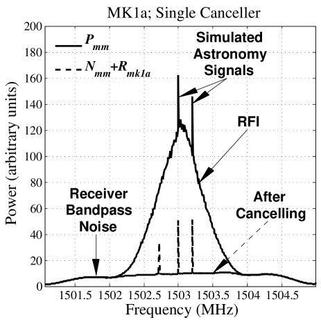
Figure 7.— Power spectra of main signal $V_{m}$ before and after MK1 cancelling with $INR_{r}\gg 1$. Two simulated cosmic signals were added at 1503.0 and 1503.2 MHz.

Figure 8 displays the power spectra of two reference signals that have had Gaussian random noise injected into their sampled voltage series, to set $\it{INR}_{r}\approx 1$ at the centre of the MW band and zero at the edges. The reason for adding the fake receiver noise was to lower the INR and accentuate any residual RFI, as detailed in (9), (10), and (13). Plots of the power spectra of the main signal (the one containing the astronomy), before and after the different cancellation techniques, are displayed in figures 9 through 12.

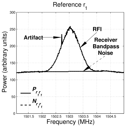
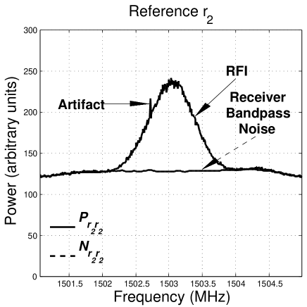
          (a)                                                              (b)

Figure 8.— Power spectra and estimated receiver noise of the reference signals. Most of the bandpass noise was artificially added to lower the INR. The peak at 1502.7 MHz is an artifact of the receiving system that leaked into the reference voltages. (a) Reference signal $V_{r_{1}}$. (b) Reference signal $V_{r_{2}}$.

Figure 9 shows unfiltered and MK1 filtered power spectra of the main astronomy voltage series. The two synthetic astronomy peaks have not been affected to any measurable level. The amount of residual power after MK1a cancelling is as expected from (7). About twice as much power has been cancelled at the centre of the RFI peak by the MK1b canceller (the added receiver noise in this case has a zero-mean cross-correlation), which is expected since $\it{INR}_{r}\approx 1$. Away from the centre of the peak, $\it{INR}_{r}$ becomes smaller and the proportion of residual RFI increases (which is why the residual RFI peak is flatter than the initial peak). No matter how long the integration is run this residual power will not decrease any further. That is, the canceller is operating in the horizontal region shown in figure 5.

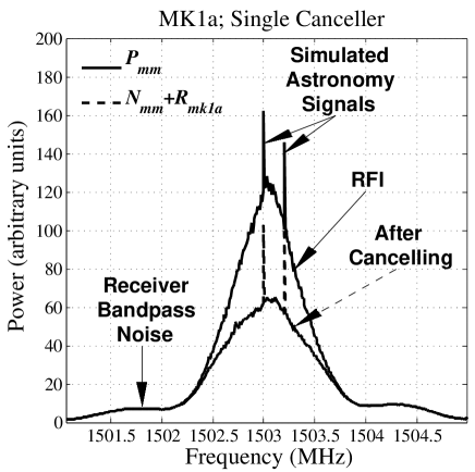
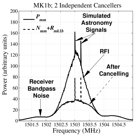
          (a)                                                              (b)

Figure 9.— Power spectra of main signal $V_{m}$ before and after MK1 cancelling. Two simulated cosmic signals were added at 1503.0 and 1503.2 MHz. (a) MK1a canceller. (b) MK1b canceller.

Before and after spectra for the MK2 cancellers are shown in figure 10. As for the MK1 cancellers, the two synthetic astronomy signals have been left unaffected. It is clear from figure 10a that when $\it{INR}_{r}<1$ the MK2a output residual power is greater than the input RFI power (except when $\it{INR}_{r}$ goes to zero, where the canceller was turned off, see section 6). This is clearly unsuitable and makes the situation worse. In contrast, the MK2b canceller (figure 10b) has removed the RFI peak down to the primary antenna’s receiver noise level, indicating that the MK2a residual power was completely added noise and not residual RFI. The removal of the RFI was extremely successful, with only a slight increase in zero-mean noise at the primary receiver noise floor, as seen in figure 11.

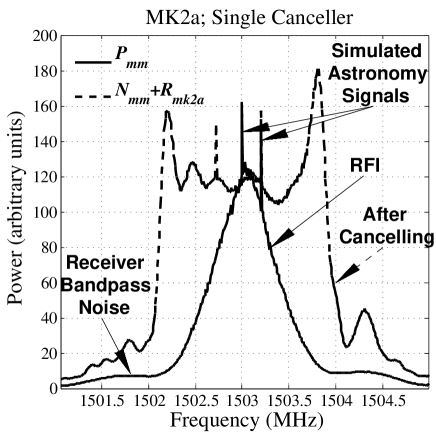
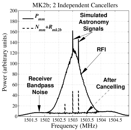
          (a)                                                              (b)

Figure 10.— Power spectra of main signal $V_{m}$ before and after MK2 cancelling. Two simulated cosmic signals were added at 1503.0 and 1503.2 MHz. (a) MK2a canceller. (b) MK2b canceller.

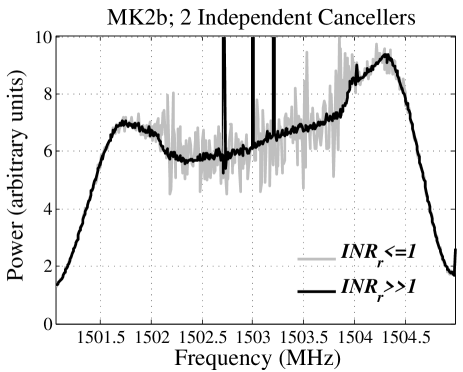
Figure 11.— MK2b canceller spectrum from figure 10b, with a $\it{INR}_{r}\gg 1$ MK2b spectrum overlaid. Very little noise is added when $\it{INR}_{r}\gg 1$, demonstrating the increase for the $\it{INR}_{r}<1$ case.

Each spectral channel in the examples in this section was averaged for 15872 samples. This means that for the MK1b and MK2b cancellers the contributed reference receiver noise power will have averaged down by about a factor of $\sqrt{15872}\approx 126$, or about 20 dB. Since the MK2b canceller output has essentially the same noise spectrum as the MK2a canceller output, but averaged down, there has been about a 20 dB reduction in unwanted power after MK2b cancelling at the centre of the RFI peak (see figure 10). This zero-mean noise would have continued to average down had we continued to integrate, and more attenuation would have been achieved. The MK1b canceller has only achieved around 6 dB of attenuation, and this will not increase with a longer integration. One should keep in mind, however, that we have inserted a substantial amount of noise into the reference voltages, which has also greatly lowered the achieved attenuation.

An important final point to note is that, with the exception of the edges of the RFI peak (where there are features associated with turning the filter off), figure 10a shows that the RFI is spread with essentially constant power over the RFI contaminated channels. This is because $\it{INR}_{r}$, which we recall is given by $G_{r}^{2}\sigma_{I}^{2}/\sigma_{N_{r}}^{2}$, is approximately proportional to $G_{m}^{2}\sigma_{I}^{2}$, so that the spectral shape of the RFI cancels out of the residual power given in (13).

5. POST-CORRELATION CANCELLERS

From an implementation point of view it is important to realise that in astronomy we are not usually seeking fast time-variable information such as modulation. In most astronomical applications the aim is to measure signal statistics since they are related to quantities such as cosmic flux density and visibilities as measured by arrays. These applications are generally either finding the auto-correlation of signals from a single antenna (to measure the power spectrum of the astronomy signal), or the cross-correlation of signals from more than one antennae (to measure the spatial coherence of the astronomy signal). See Thomson et al. (1986) and various chapters of Taylor et al. (1999) for an overview. In this paper we have concentrated on the power spectra given by auto-correlations, however all of the techniques discussed can be generalised to work on cross-correlations.

The upshot of only requiring signal statistics is that if the canceller weights are not changing appreciably over the 100 millisecond or so time interval that the statistics are measured over, then the algorithms can be applied to the statistics rather than each voltage series. This means that they are applied at a rate of Hz to kHz rather that MHz to GHz. It also means that if the new astronomical cross-correlators that are coming online for new and existing facilities have a few extra inputs for reference antennae, then no new filters need to be added to the signal paths, and the cancellation can be performed after the observation as part of post-processing. For a comparison of voltage cancellation and statistics cancellation for RFI signals that require filters with weights that are changing appreciably during an integration, see Mitchell & Robertson (2005).

The standard statistics canceller used in radio astronomy is a post-correlation version of the MK2b canceller discussed in section 2.3. If we use $P_{jk}$ to denote the correlation between signals from antennae $j$ and $k$, the quantity that is subtracted from the auto-correlation of antenna $m$ is determined from amplitude and phase closure relations (Briggs et al., 2000):

$$C_{\it{pc2}}=\frac{P_{mr_{1}}P^{*}_{mr_{2}}}{P^{*}_{r_{1}r_{2}}}\approx|G_{m}|^{2}\sigma_{I}^{2}.$$ (16)

Since the reference signal does not contain any information about the astronomy signal, it will not be present in any of the quantities in (16). The denominator removes the reference signal RFI’s phase and amplitude information from the numerator, leaving information about the RFI in the signal from antenna $m$, and zero-mean noise, since the expectation operators are not infinite in extent. When $C_{\it{pc2}}$ is subtracted from main signal power $P_{mm}$, the mean residual power is (see Mitchell 2004)

$$R_{\it{pc2}}=\frac{G_{m}^{2}\sigma_{I}^{2}}{\sqrt{\it{INR}_{r_{1}}\it{INR}_{r_{2}}}\sqrt{\Delta\nu\tau_{\it{int}}}},\\$$ (17)

as in (14). $R_{\it{pc2}}$ is shown in figure 12. As long as the gain and geometric delay stay essentially constant over the time average, the “pre” and “post” correlation techniques are very similar; $R_{\it{pc2}}\approx R_{\it{mk2b}}$.

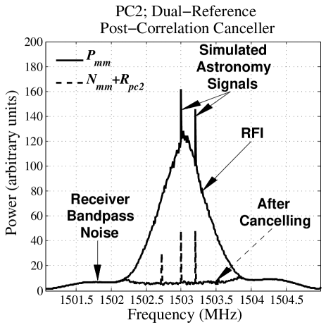
Figure 12.— Power spectra of main signal $V_{m}$ before and after post-correlation cancelling. Two simulated cosmic signals were added at 1503.0 and 1503.2 MHz. There are slight artifacts at the edge of the peak where $\it{INR}_{r}\rightarrow 0$ and the canceller is turning off, as described in section 6.

While in the last few sections an extreme case has be demonstrated (that of a low reference INR), it does highlight major differences between the different cancellers. The main differences being that infinite RFI removal is theoretically possible for cancellers that use two reference signals, but not for single reference cancellers. It is also clear that when the weights are slowly varying, the post-correlation canceller is equivalent to the dual-reference MK2b canceller.

Another way in which the MK2b and post-correlation canceller techniques can differ is in their instabilities at low INR levels. Equations (12) and (16) have denominators that become zero-mean noise when there is no correlated RFI signal, which can lead to numerical errors. The coefficients of the single-reference techniques go to zero when the RFI becomes weak and the cancellers automatically turn off. These issues are discussed next.

6. INSTABILITIES IN THE DUAL REFERENCE ALGORITHMS

Equations (12) and (16) show that the dual-reference cancellers can have stability problems when $\it{INR}_{r}\ll 1$. In frequency channels where the correlated interference is zero or very small, (12) and (16) are noise dominated and can result in a division by zero (or very close to zero). This cannot occur in the MK1 cancellers since (6) goes to zero as $I\rightarrow 0$ and they turn off. A modified post-correlation canceller has been suggested by Briggs et al. (2000) in which an extra term is added to the denominator of (16):

$$C_{\it{pc2}}^{\prime}=\frac{P_{mr_{1}}P^{*}_{mr_{2}}P_{r_{1}r_{2}}}{\Psi^{2}+P^{*}_{r_{1}r_{2}}P_{r_{1}r_{2}}},$$ (18)

where $\Psi=\left(\left<N_{r_{1}}N^{*}_{r_{1}}\right>\left<N_{r_{2}}N^{*}_{r_{2}}\right>/\Delta\nu\tau_{\it{int}}\right)^{1/2}$, which is an estimate of the noise power in the reference cross-correlation, and the prime indicates that $C_{\it{pc2}}$ has been approximated. The extra term $\Psi^{2}$ stops the zero-mean fluctuations in $P_{r_{1}r_{2}}$ from going too close to zero, while for large $\it{INR}_{r}$ equation (18) reduces to (16).

Since $\Psi^{2}$ introduces a small bias in a similar way to the MK1 cancellers, a relation equivalent to (7), but with a much smaller bias, can be derived:

$$R_{\it{pc2}}^{\prime}\approx\frac{G_{m}^{2}\sigma_{I}^{2}}{1+\it{INR}_{1}\it{INR}_{2}\Delta\nu\tau_{\it{int}}},$$ (19)

This will have both a noise and a RFI component, as in (7), however, since the canceller is now biased like a MK1a canceller the added receiver noise term will not average away. $R_{\it{pc2}}^{\prime}$ reduces as $\it{INR}^{2}$ multiplied by the number of samples in the time average.

There is a similar problem for the pre-correlation MK2 adaptive cancellers. In the lag domain, the division in (12) becomes a multiplication by the inverse of a matrix with columns containing offset copies of the $r_{1}$-$r_{2}$ cross-correlation function (Widrow & Stearns, 1985). Divisions by zero in the frequency domain due to interference-free frequency channels in $P_{r_{1}r_{2}}$ are manifest in the reference lag matrix as singular values. One method of dealing with this is to use singular value decomposition to decompose the matrix into two orthonormal triangular matrices and one diagonal matrix (see $\S$ 2.9 of Press et al. 1986). Singular (or near-singular) values can be selected when the relevant diagonal matrix elements are less than a chosen threshold, such as $\Psi$. The singular parts of the matrix contain no information about the correlated signal and are removed from the decomposition matrices. The inverse matrix can then be reconstructed from the remaining parts of the three decomposition matrices, and it will not function in the RFI-free parts of the spectrum.

7. SUMMARY

Interference cancelling using a single reference antenna can give excellent results when the reference signal interference-to-noise ratio is large, and there is more gain towards the interfering signal for the reference antenna than for the astronomy antennae. However, receiver noise in the reference signal means that a fraction of the interference will always remain after cancelling. A second reference signal can be used to remove the noise bias and give infinite interference attenuation, but a larger amount of reference receiver noise is added during cancelling. For pre-correlation systems, a dual canceller setup can be used to average the (zero-mean) receiver noise away, a process that comes automatically with post-correlation cancellers. A breakdown of the main properties for the different mitigation techniques is given in table 1.

It is important to note that even though the single-reference cancellers leave residual RFI, the residual may be extremely small and well below the RMS noise. This occurs when the interference-to-noise ratios of the reference signals are very large, and the use of two references (in pre-correlation systems) might just add complexity to the system with little or no benefit. However, if maximum sensitivity is required, one should be aware that they will eventually reach a non-zero residual signal.

Using two reference signals to remove the reference receiver noise bias removes the inherent stability of the algorithms in situations where some or all of the frequency channels are interference-free. Although there are applications in which the passband will always be entirely filled with RFI (such as observations in the GPS L1 and L2 bands), many interfering signals will only take up a part of the band. In these cases the algorithms need a mechanism to turn themselves off in the vacant frequency channels.

	Fig. no.	Ref. Ants.	Filters	Configuration	Behaviour	Eqn. no.
MK1a	1	1	1	One reference antenna feeds both filter and weight generator.	Minimises residual power, but includes some RFI. Turns off gracefully as $INR_{r}\rightarrow 0$.	7, 9, 10
MK2a	2	2	1	Independent reference antennae for filter and weight generator.	Totally cancels RFI, but adds extra noise. Must be controlled as $INR_{r}\rightarrow 0$.	13
MK1b	4	2	2	Two MK1a cancellers, operating on copies of main signal.	Sensitivity decrease, and non-zero RFI floor.	15
MK2b	3	2	2	Two MK2a cancellers, operating on copies of main signal.	Sensitivity decrease, but no non-zero RFI floor.	14
PC2	not shown	2	1	Two reference correlations with each astronomy signal.	Sensitivity decrease, but no non-zero RFI floor. Must be controlled as $INR_{r}\rightarrow 0$.	17, 19

Table 1Summary of the main properties for various interference mitigation techniques

References

- Barnbaum & Bradley (1998) Barnbaum, C., & Bradley R. F. 1998, AJ, 116, 2598
- Bell et al. (2001) Bell, J. F., et al. 2001, PASA, 18, 105
- Bower (2001) Bower, G. C. 2001, ATA Memo 31.
- Briggs et al. (2000) Briggs, F. H., Bell, J. F., & Kesteven M. J. 2000, AJ, 120, 3351
-
Mitchell (2004)
Mitchell, D. A. 2004,
Ph.D. Thesis,
Interference Mitigation in Radio Astronomy,
The University of Sydney,
http://setis.library.usyd.edu.au. - Mitchell & Bower (2001) Mitchell, D. A., & Bower, G. C. 2001, ATA Memo 36
- Mitchell & Robertson (2005) Mitchell, D. A., & Robertson, J. G. 2005, RS, special section on Interference Mitigation, in press
- Press et al. (1986) Press, W. H., Flannery, B. P., Teukolsky, S. A., & Vetterling, W. T. 1986, NUMERICAL RECIPES. The Art of Scientific Computing, (Cambridge University Press)
- MATLAB User’s Guide (1998) The Mathworks, Inc. 1998, MATLAB User’s Guide, (The Mathworks, Inc.)
- Taylor et al. (1999) Taylor, G. B., Perley, R. A., & Carilli, C. L., ed. 1999, PASP, 180
- Thomson et al. (1986) Thompson, A. R., Moran, J. M., & Swenson, G. W. 1986, Interferometry and Synthesis in Radio Astronomy, (New York: Wiley-Interscience)
- Widrow & Stearns (1985) Widrow, B., & Stearns, S. D. 1985, Adaptive Signal Processing, Englewood Cliffs, NJ: Prentice Hall)