Temperature and Polarization Patterns in Anisotropic Cosmologies

Abstract

We study the coherent temperature and polarization patterns produced in homogeneous but anisotropic cosmological models. We show results for all Bianchi types with a Friedman-Robertson-Walker limit (i.e. Types I, V, VII₀, VII_h and IX) to illustrate the range of possible behaviour. We discuss the role of spatial curvature, shear and rotation in the geodesic equations for each model and establish some basic results concerning the symmetries of the patterns produced. We also give examples of the time-evolution of these patterns in terms of the Stokes parameters $I$, $Q$ and $U$.

1 Introduction

Precise measurements of the temperature anisotropies of the Cosmic Microwave Background (CMB), particularly those from the Wilkinson Microwave Anisotropy Probe (WMAP) [1, 2], form the sturdiest foundations of the current (“concordance”) cosmological model describing a universe dominated by cold dark matter (CDM) and a cosmological constant [3], and therefore known as $\Lambda$CDM for short. It is an essential component of this model that the primordial metric perturbations that gave rise to the galaxies and large-scale structure we observe around us today should be Gaussian and statistically homogeneous (i.e. stationary) [4, 5, 6] and this means that the temperature fluctuations observed in the CMB should be Gaussian and statistically isotropic.

Detailed analysis of the WMAP data has shown that any departures from the standard framework are small and of uncertain statistical significance. Although some anomalous behaviour has been reported [7], there remains no clear evidence of primordial non-Gaussianity, but there are several indications of departures from statistical anistropy across the CMB sky. Among the interesting phenomena revealed by detailed analyses of the pattern of CMB temperature fluctuations are an extremely cold spot [8, 9, 10, 11, 12, 13, 14], unusual alignments between large-scale harmonic modes of the temperature pattern [15, 16, 17, 18, 19, 20, 21, 22, 23, 24, 25] (sometimes dubbed “The Axis of Evil”) and a global hemispherical power asymmetry [26, 27, 28, 29, 30].

One must not get carried away with the these features because they are - almost without exception - based on a posteriori evaluations of statistical significance. If the occurrence of an anomalous feature $A$ in a given model $M$ is $P(A|M)\simeq 0.001$ (say) then that does not necessarily mean that the probability of the model given that the anomaly is observed $P(M|A)$ is similarly low. One has to take into account all the other data that are not anomalous before deciding on a true measure of the significance of a departure. Attempts to do this rigorously have generally confirmed that current observations are not sufficiently compelling to suggest that the standard model needs to be abandoned [31, 32, 33, 34]. Moreover, other analyses suggest the further possibility that the WMAP temperature fluctuations may be affected by foregrounds or other systematic problems [35, 36, 37, 38]. Even slight effects of this type could seriously hamper our attempts to uncover evidence of physics beyond the standard model.

But, although the evidence for the examples of global asymmetry discussed above is by no means overwhelming, taken together they do at least suggest the possibility that we may live in universe which is described by a background cosmology that is globally anisotropic, i.e. one not described by a Friedmann-Robertson-Walker (FRW) model and it is therefore incumbent upon us to consider alternatives to the standard model in order to learn best how to use the data to confirm or rule out variations on the standard cosmology.

The approach we follow here is to study the Bianchi models, i.e. cosmological models based on exact solutions to Einstein’s General Theory of Relativity involving homogeneous but not necessarily isotropic spatial sections. The Bianchi classification groups all possible spatially homogeneous but anisotropic relativistic cosmological models into types depending on the symmetry properties of their spatial hypersurfaces [39, 40]; we discuss these models in more detail later in the paper.

The Bianchi models are not particularly strongly motivated from the point of view of fundamental physics, but do nevertheless represent a promising and potentially profitable first step away from the standard cosmological framework. For example, it has been known for some time that interesting localized features in the CMB temperature pattern can occur in Bianchi models with negative spatial curvature [41, 42, 43, 44, 45, 46]. The physical origin of such features lies in the focussing effect of space on the geodesics that squeezes the pattern of the anisotropic radiation field into a small region of the sky. The observed lack of large-scale asymmetries in the CMB temperature has in the past been used to place constraints on the global rotation and shear allowed in Bianchi models [46, 47, 48]. More recently, however, attention has shifted to the possibility of using the additional parameters available in such models to reproduce a cold spot such as that claimed to exist in the WMAP data. Since we now know that our Universe is close to isotropic, attention has focussed on the subset of the Bianchi types that contain the FRW model as a limiting case.The model which appears to best able to reproduce the anomalous cold spot is the Bianchi VII_h case [49, 50, 51, 52, 53], although Bianch V also has negatively curved spatial sections and can therefore, in principle, also produce localised features [55].

However, as well as forming distinctive features in the temperature pattern, anisotropic cosmological models also generate characteristic signatures in the polarized component of the background radiation. Thomson scattering generates polarization as long as there is a quadrupole anisotropy in the temperature field of the radiation incident upon the scattering particle. In the concordance cosmology the temperature and polarization patterns are (correlated) stochastic fields arising from their common source in scalar and tensor perturbations arising from inflation. In a Bianchi cosmology, however, the patterns are coherent and have a deterministic relationship to one another owing to their common geometric origin. It has recently been shown [55, 56, 57] that only in special cases are the properties of the polarization field produced in Bianchi VII_h consistent with the latest available WMAP polarization data [58] because such models generally involve a large odd-parity (B-mode) [59, 60] contribution that exceeds the experimental upper limit. For a discussion of CMB polarization in the context of the so-called Axis of Evil, see ref. [61].

But their ability to produce localized features is not the only reason to be interested in the temperature and polarization patterns produced in Bianchi models. For example, history provides a host of connections between these models and the understanding of the interaction between electromagnetic radiation and gravitational waves [62, 63, 64, 65, 66, 67].

Our aim in this paper is to give a relatively gentle introduction to the Bianchi models and show how to calculate the temperature and polarization properties of the radiation field expected to arise within them, using methods outlined in a previous short paper [55]. Our aim in doing this is neither to provide an exhaustive set of alternatives to the standard cosmology nor to perform a detailed statistical analysis of the patterns we calculate. Instead we plan to elucidate some of the general properties of the radiation field in anisotropic cosmological models belonging to the different Bianchi types.

The outline is as follows. In the next section we describe the Bianchi classification in general terms for the benefit of the non-expert. In Section 3 we introduce the specific formalism of Bianchi cosmological models, i.e. exact solutions of the Einstein equations involving space-times with symmetries described by the various Bianchi types. In Section 4 we explain how we compute the radiation patterns in these models and then, in Section 5, show examples of the results obtained. We summarize and present our conclusions in Section 6.

2 Bianchi Spaces

In the Friedman models on which the standard Big Bang cosmology is based, hypersurfaces of constant time are defined to be those on which the matter density is the same throughout space. We can construct a more general definition of homogeneity by requiring that all comoving observers see essentially the same version of cosmic history. In mathematical terms this means that there must be some symmetry that relates what the Universe looks like as seen by observer A to what is seen in a coordinate system centred on any other observer B. The possibly space-times consistent with this requirement possess symmetries can be classified into the various Bianchi types, which we now discuss. For more details, see [68, 69].

The Bianchi classification is based on the construction of space-like hypersurfaces upon which it is possible to define at least three independent vector fields, $\xi_{\alpha}$, that satisfy the Killing’s equation

$$\xi_{i;j}+\xi_{j;i}=0.$$ (1)

The vectors that satisfy this are called Killing vectors; the semicolons denote covariant derivatives. Suppose the Killing vectors are denoted $\xi_{\alpha}$, where Greek indices can run from $0$ to $3$. The commutators of the ${\bf\xi}_{\alpha}$ are defined by

$$[\xi_{\alpha},\xi_{\beta}]\equiv\xi_{\alpha}\xi_{\beta}-\xi_{\beta}\xi_{\alpha}=C_{\alpha\beta}^{\delta}\xi_{\delta},$$ (2)

where the $C_{\alpha\beta}^{\delta}$ are called structure constants. These are antisymmetric, in the sense that,

$$C_{\alpha\beta}^{\delta}=-C_{\beta\alpha}^{\delta}.$$ (3)

One can understand how the structure constants arise by considering symmetry transformations. In three dimensions, spatial homogeneity is relates to the existence of three independent sets of curves with tangent vectors $\xi_{\alpha}$. An infinitesimal symmetry transformation takes an arbitrary point P (with coordinates $x_{i}$) to the point P^′ with coordinates $x_{i}+\delta x_{i}$, where

$$\delta{\bf x}={\bf\xi}_{\rm P}\delta t$$ (4)

for $\xi_{\rm P}$ some linear combination of the $\xi_{\alpha}$ defined at P. The same symmetry transformation takes the tip of an arbitrary infinitesimal vector ${\bf\zeta}_{\rm P}\delta s$ at P to a new position ${\bf\xi}_{{\rm P}+{\bf\zeta}_{\rm P}\delta s}\delta t$ at $P^{\prime}$. This means that

$${\bf\zeta}_{\rm{P}}\delta s\rightarrow{\bf\zeta}^{\prime}_{P^{\prime}}\delta s={\bf\zeta}_{\rm P}\delta s+\xi_{{\rm P}+{\bf\zeta}_{\rm P}\delta s}\delta t-{\bf\xi}_{\rm P}\delta t.$$ (5)

It is now possible to compare the transformed vector ${\bf\zeta}^{\prime}_{{\rm P}^{\prime}}$ with ${\bf\zeta}_{\rm P^{\prime}}$, the ‘actual’ vector field defined at P^′. The difference between the two vectors is the Lie derivative of ${\bf\zeta}$ taken along ${\bf\xi}$:

$$\mathcal{L}_{\bf\xi}{\bf\zeta}\equiv\lim_{\delta t\rightarrow 0}\frac{{\bf\zeta}^{\prime}_{{\rm P}^{\prime}}-{\bf\zeta}_{\rm P}}{\delta t}={\bf\xi}\cdot{\bf\nabla}{\bf\zeta}-{\bf\zeta}\cdot{\bf\nabla}{\bf\xi}.$$ (6)

This tells us, roughly speaking, by how much we must turn a vector after it is carried by a symmetry transformation from P to P^′ in order for it to point in the same direction as it did before the transformation.

Instead of choosing an arbitrary vector we can now take one of the $\xi_{\alpha}$, and instead of an arbitrary direction we transform it along another of the $\xi_{\alpha}$. The type of space is specified by the Lie derivatives obtained for this type of operation:

$$\mathcal{L}_{{\bf\xi}_{\beta}}{\bf\xi}_{\alpha}=C_{\alpha\beta}^{\delta}{\bf\xi}_{\delta};$$ (7)

since it is defined as the difference between two vectors the Lie derivative must itself be a vector and so it can be expressed as a linear combination of the three independent basis vectors. This gives us the structure constants we described above.

The set of $n$ Killing vectors will have some $n$-dimensional group structure, say $G_{n}$, that depends on the equivalence classes of the structure constants $C_{\alpha\beta}^{\delta}$. This is used to classify all spatially homogeneous cosmological models. The most useful form of this classification proceeds as follows. On any particular spacelike hypersurface, the Killing vector basis can be chosen so that the structure constants can be decomposed as

$$C_{\alpha\beta}^{\eta}=\epsilon_{\alpha\beta\gamma}n^{\gamma\eta}+\delta_{\beta}^{\eta}a_{\alpha}-\delta_{\alpha}^{\eta}a_{\beta},$$ (8)

where $\epsilon_{\alpha\beta\gamma}$ is the total antisymmetric tensor and $\delta_{\alpha}^{\beta}$ is the Kronecker delta. The tensor $n^{\alpha\beta}$ is diagonal with entries, say, $n_{1}$, $n_{2}$, and $n_{3}$. The vector $a_{\alpha}=(a,0,0)$ for some constant $a$. All the parameters $a$ and $n_{\alpha}$ can be normalized to be $\pm 1$ or zero. If $an_{2}n_{3}=0$ then $n_{2}$ and $n_{3}$ can be set to $\pm 1$ and $a$ is then conventionally taken to be $\sqrt{|h|}$ where $h$ is a parameter used in the classification. The possible combinations of $n_{1}$ and $a$ then fix the different Bianchi types according to the table.

Bianchi Type	Class	$a$	$n_{1}$	$n_{2}$	$n_{3}$
I	A	0	0	0	0
II	A	0	+	0	0
VI0	A	0	0	+	-
VII0	A	0	0	+	+
VIII	A	0	-	+	+
IX	A	0	+	+	+
IV	B	+	0	0	+
V	B	+	0	0	0
VIh	B	+	0	+	-
VIIh	B	+	0	+	+

Table 1: The Bianchi types shown in terms of whether the various parameters used to construct the classification are zero, positive or negative; the designation of Class A or Class B depends on whether $a=0$, or not, respectively. The parameter $h$ is defined by $h=a^{2}/n_{1}n_{2}$. The spaces of particular interest in this paper are I, V, VII₀, VII_h and IX because these contain the isotropic FRW spaces as limiting cases; the others are shown just for completeness.

It is interesting also to think about the generality of the different types. This can be expressed in terms of the dimension $p$ of the Bianchi group, which gives the dimension of the orbit of $C_{\alpha\beta}^{\delta}$ as a subset of all 9 of the distinct components. The Killing vectors must satisfy the Jacobi identities, so

$$\epsilon^{\alpha\beta\gamma}\left[[\xi_{\alpha},\xi_{\beta}],\xi_{\gamma}\right]=0.$$ (9)

This implies that

$$n^{\alpha\beta}a_{\beta}=0,$$ (10)

so that the orbits of any particular group type are at most six-dimensional. The (isotropic) spaces that feature in the Friedman models have $G_{6}$ symmetry groups with $G_{3}$ subgroups, so that the zero curvature ($K=0$) FRW model can be thought of as a special case of Bianchi Types I or VII₀. Likewise the open ($K<0$) FRW model is a special case of types V or VII_h. The closed FRW case ($K>0$) is a special case of Bianchi type IX.

We are interested in cosmological models that are close to the completely isotropic case described by the FRW metric, but not all the Bianchi types contain this as a special limiting case [40, 39]. Those that do are types I, V, VII₀, VII_h and IX; we do not discuss the other cases any further in this paper. Bianchi I and Bianchi VII₀ are spatially flat, Bianchi IX is positively curved and Bianchi types V and VII_h have negative spatial curvature. The “open” (i.e. negatively curved) cases are of particular interest as they permit the focussing of anisotropic patterns into small regions of the sky. The scalar curvature $R$ of the spatial sections which is given in terms of the Bianchi parameters as the following convenient form

$$R=\frac{1}{2}(2n_{1}n_{2}+2n_{1}n_{3}+2n_{2}n_{3}-n^{2}_{1}-n^{2}_{2}-n^{2}_{3})-6a^{2}$$ (11)

For Bianchi V we have $n_{1}=n_{2}=n_{3}=0$ so that $R=-6a^{2}$. In Bianchi VII_h we have $n_{1}=0$ but $n_{2}\neq 0$ and $n_{3}\neq 0$; the parameter $h$ is defined by $h=a^{2}/n_{2}n_{3}$, it is related to the parameter $x$ which defines the ’spiralness’ of the temperature patterns,

$$x=\sqrt{\frac{h}{1-\Omega_{0}}}$$ (12)

For reference, the scalar curvatures of all the models we discuss hereafter are shown in Table 2.

Type	$R$	K
$I$	0	0	Flat
$V$	$-6a^{2}$	$<0$	Open
$VII_{0}$	$-\frac{1}{2}(n_{2}-n_{3})^{2}$	$0$	Flat
$VII_{h}$	$-6a^{2}-\frac{1}{2}(n_{2}-n_{3})^{2}$	$<0$	Open
$IX$	$n_{1}n_{2}+n_{1}n_{3}+n_{2}n_{3}-\frac{1}{2}(n_{1}^{2}+n_{2}^{2}+n_{3}^{2})$	$>0$	Closed

Table 2: Dependence of the scalar curvature $R$ on the parameters $a$ and $n_{i}$ involved in the construction of the Bianchi classification for those models with an FRW limit.

3 Bianchi Cosmologies

3.1 Basics

The models we consider are based on Einstein’s general theory of relativity and we use the field equations in the form

$$G_{ab}\equiv R_{ab}-\frac{1}{2}Rg_{ab}=T_{ab}-\Lambda g_{ab},$$ (13)

with $R_{ab}$ being the Ricci Tensor, $R$ the Ricci scalar, $T_{ab}$ the energy-momentum tensor and $\Lambda$ the cosmological constant. Indices $a$ and $b$ run from $0$ to $3$ (c.f. $i$, $j$ and $\alpha$, $\beta$ which run from $1$ to $3$). We use units where $8\pi G=c=1$. In terms of a coordinate system $x^{a}$, the metric $g_{ab}$ is written

$$ds^{2}=g_{ab}dx^{a}dx^{b}=(h_{ab}-u_{a}u_{b})dx^{a}dx^{b},$$ (14)

where $u^{a}$ is the fluid velocity; the signature of $g_{ab}$ is $(-+++)$. As we have already explained, the components of the metric $g_{ab}$ describing a Bianchi space are invariant under the isometry generated by infinitesimal translations of the Killing vector fields. In other words, the time-dependence of the metric is the same at all points. The Einstein equations relate the energy-momentum tensor $T_{ab}$ to the derivatives of $g_{ab}$ so if the metric is invariant under a given set of operations then so are the physical properties encoded in $T_{ab}$.

Before proceeding further, let us comment further on the degree of generality of the various Bianchi models which we touched on in the previous section. An alternative way to quantify this, rather than looking at the group structure, is to work out the number of arbitrary constants needed to specify the solutions. This seems more interesting from a physical point of view, as we are interested in the solutions to the field equations rather than the groups themselves. The number of arbitrary constants depends on the form of the energy-momentum tensor. In Table 3 we give the results for vacuum and perfect fluid equations of state. The appearance of $h=-1/9$ as a special case in this table relates to the fact that two of the Einstein constraint equations become null identities for this particular choice of $h$. From the Table it emerges that the “most general” vacuum solutions are types VII_h, VI_h, VIII, VI_h=-1/9 and IX, all of which have four arbitrary parameters. The least general is the Bianchi Type I vacuum solution, which has only one.

Bianchi Type	Group Dimension	Vacuum	Fluid
	$p$	$r$	$s$
I	0	1	2
II	3	2	5
VI0	5	3	7
VII0	6	4	8
VIII	6	4	8
IX	6	4	8
IV	5	3	7
V	3	1	5
VIh	6	4	8
VIIh	6	4	8
VIh=-1/9	6	4	7

Table 3: The Bianchi types shown in terms of the group dimension $p$ and number of arbitrary constants needed to specify the model on a given constant time surface, in vacuum ($r$) and with a perfect fluid equation of state ($s$).

For cases describing perfect fluids the situation is a little more subtle. One would expect to have four additional parameters to specify these compared to the vacuum solutions, but the table shows that $s=r+4$ is not always the case. This is the case because the Einstein equations place additional restrictions on the form of $T_{ab}$ allowed in Types I and II. For example, if a perfect fluid is added to the vacuum Type I solution then the form of the metric requires all the time-space components of the Ricci tensor to be identically zero. This means that the energy-momentum tensor $T_{ab}$ must have

$$T_{0\alpha}=0$$ (15)

for $\alpha=1$, $2$ or $3$. This in turn means that the matter must be comoving, i.e. its velocity is $u_{a}=\delta_{a}^{0}$. Only one free parameter is therefore needed to specify the solution, the energy density $\mu$. The perfect fluid case of Bianchi VI_h=-1/9 is also peculiar, in that it is not as general as Bianchi VI_h, VII_h, VIII or IX because the degeneracy described above only appears in vacuum.

3.2 Example: The Kasner Solution

General solutions in closed form of the Einstein equations are only known for some special cases of the Bianchi types, which demonstrates the difficulty of finding meaningful exact solutions in situations of restricted symmetry. There is, however, one very well known example - the Kasner solution [74]- which is a useful illustration of the sort of behaviour one can obtain and which therefore provides a useful pedagogical route into a more general treatment of Bianchi cosmologies.

The Kasner metric, which describes a space belonging to Bianchi Type I, has the form

$$ds^{2}=dt^{2}-X_{1}^{2}(t)dx_{1}^{2}-X_{2}^{2}dx_{2}^{2}-X_{3}^{2}dx_{3}^{2}.$$ (16)

Substituting this metric into the Einstein equations (with $\Lambda=0$ and a perfect fluid with pressure $p$ and density $\mu$) yields

$$\frac{\ddot{X_{i}}}{X_{i}}-\left(\frac{\dot{X_{i}}}{X_{i}}\right)^{2}+3\left(\frac{\dot{X_{i}}}{X_{i}}\right)\left(\frac{\dot{a}}{a}\right)=\frac{1}{2}\left(\mu-p\right),$$ (17)

in which $a^{3}=X_{1}X_{2}X_{3}$. Note that this emerges from the diagonal part of the Einstein equations so the summation convention does not apply. One also obtains

$$\frac{\dot{X_{1}}\dot{X_{2}}}{X_{1}X_{2}}+\frac{\dot{X_{2}}\dot{X_{3}}}{X_{2}X_{3}}+\frac{\dot{X_{3}}\dot{X_{1}}}{X_{3}X_{1}}=\mu.$$ (18)

This is easy to interpret: the spatial sections expand at a rate $\dot{X_{i}}/X_{i}$ in each direction. The mean rate of expansion is just

$$\frac{\dot{a}}{a}=\frac{1}{3}\left(\frac{\dot{X_{1}}}{X_{1}}+\frac{\dot{X_{2}}}{X_{2}}+\frac{\dot{X_{3}}}{X_{3}}\right).$$ (19)

In the neighbourhood of an observer at the centre of a coordinate system $x_{i}$, fluid particles will move with some velocity $u_{i}$. In general,

$$\frac{\partial u_{i}}{\partial x_{j}}=\frac{1}{2}\left(\frac{\partial u_{i}}{\partial x_{j}}-\frac{\partial u_{j}}{\partial x_{i}}\right)+\frac{1}{2}\left(\frac{\partial u_{i}}{\partial x_{j}}+\frac{\partial u_{j}}{\partial x_{i}}\right)=\omega_{ij}+\theta_{ij},$$ (20)

where $\omega_{ij}$ is the rate of rotation: in more familiar language, the vorticity vector $\omega_{i}=\epsilon_{ijk}\omega_{jk}$ which is just the curl of $u_{i}$. The tensor $\theta_{ij}$ can be decomposed into a diagonal part and a trace-free part according to

$$\theta_{ij}=\frac{1}{3}\delta_{ij}\theta+\sigma_{ij},$$ (21)

where $\sigma_{ii}=0$. In this description $\theta$, $\sigma_{ij}$ and $\omega_{ij}$ respectively represent the expansion, shear and rotation of a fluid element. In the Kasner model we have

$$\theta=3(\dot{a}/a)$$ (22)

and

$$\omega_{ij}=0.$$ (23)

As we shall see below, more complicated Bianchi models have non-zero rotation. We can further write evolution equations for

$$\sigma_{i}=\frac{\dot{X_{i}}}{X_{i}}-\frac{\dot{a}}{a}.$$ (24)

In particular we get

$$\dot{\sigma_{i}}+\theta\sigma_{i}=0$$ (25)

which can be immediately integrated to give

$$\sigma_{i}=\frac{\Sigma_{i}}{a^{3}},$$ (26)

where the $\Sigma_{i}$ are constants such that $\Sigma_{1}+\Sigma_{2}+\Sigma_{3}=0$. The Kasner solution itself is for a vacuum $p=\mu=0$, which has a particularly simple behaviour described by $X_{i}=A_{i}t^{p}$ where $p_{1}+p_{2}+p_{3}=p_{1}^{2}+p_{2}^{2}+p_{3}^{2}=1$. Notice that in general these models possess a shear that decreases with time. They therefore tend to behave more like an FRW model as time goes on. Their behaviour as $t\rightarrow 0$ is, however, quite complicated and interesting.

3.3 Tetrad Frame

It is convenient to follow [40], introducing a tetrad basis constructed From a local coordinate system $x^{i}$ by

$${\bf e}_{a}=e_{a}^{i}\frac{\partial}{\partial x^{i}}$$ (27)

such that

$$g_{ab}=e_{a}^{i}e_{b}^{j}g_{ij}=e_{a}^{i}e_{bi}={\rm diag}(-1,+1,+1,+1)$$ (28)

meaning that the tetrad basis ${\bf e}_{a}$ is orthonormal. The Ricci rotation coefficients,

$$\Gamma_{abc}=e_{a}^{i}e_{ci;j}e_{b}^{j},$$ (29)

are the tetrad components of the Christoffel symbols; semicolons denote covariant derivatives. In general, the operators defined by equation (27) do not commute: they generate a set of relations of the form

$$[{\bf e}_{a},{\bf e}_{b}]=\gamma_{ab}^{c}{\bf e}_{c}.$$ (30)

These Ricci rotation coefficients are just

$$\Gamma_{abc}=\frac{1}{2}(\gamma_{abc}+\gamma_{cab}-\gamma_{bca}).$$ (31)

The matter flow is described in terms of the expansion $\vartheta_{ab}$ and shear $\sigma_{ab}$:

$$u_{a;b} = \omega_{ab}+\vartheta_{ab}-\dot{u}_{a}u_{b}$$

$$\sigma_{ab} = \vartheta_{ab}-\frac{1}{3}\vartheta h_{ab}\equiv\vartheta_{ab}-Hh_{ab},$$ (32)

where $\vartheta=\Tr(\vartheta_{ab})=\vartheta_{aa}$ and the magnitude of the shear is $\sigma^{2}=\sigma^{ab}\sigma_{ab}/2$. We now take the time-like vector in our basis to be the fluid flow velocity so that $u^{a}=\delta_{0}^{a}$ and $u_{a}=-\delta_{a}^{0}$. The remaining space-like vectors form an orthonormal triad, with a set of commutation relations like that shown in equation (30) but with an explicit time dependence in the “structure constants” describing the spatial sections:

$$[{\bf e}_{i},{\bf e}_{j}]=\gamma_{ij}^{k}(t){\bf e}_{k}.$$ (33)

Without loss of generality we can write

$$\gamma_{ij}^{k}=\epsilon_{ijl}n^{lk}+\delta_{j}^{k}a_{i}-\delta_{i}^{k}a_{j},$$ (34)

for some tensor $n_{ij}$ and some vector $a_{i}$. The Jacobi identities require that $n_{ij}a^{j}=0$ so we choose $a^{j}=(a,0,0)$ and $n_{ij}={\rm diag}(n_{1},n_{2},n_{3})$. The four remaining free parameters are used to construct the Bianchi classification described briefly above, and more in detail elsewhere [39, 40, 70, 71, 72, 73].

4 Radiation Transport in Anisotropic Cosmologies

Having established some general results about Bianchi models, we now turn to the problem of calculating the temperature and polarization patterns they produce. Our general method is to generalize the Liouville equation so that it can be applied to a complete description of photons travelling through a curved space-time. This requires that we set up radiation distribution functions that incorporate all the Stokes parameters needed to specific polarized radiation. We also need to include a source term that describes the effects of Thomson scattering by free electrons for the entire history from decoupling to the observed epoch. In doing this we follow closely the methods of [42] and also [43]. Note, however, that they use a different definition of the Ricci rotation coefficients.

4.1 Radiation Description

Our expansion of the distribution functions into multipoles is based on the usual Stokes parameters, and on spin-weighted spherical harmonics. The transfer equation for polarized radiation propagating through space-time can be described by a (complex) photon distribution comprising components with spin-weights 0 and 2, i.e.

$$\hat{N}\equiv{N^{0}\choose N^{2}}=\frac{1}{ch^{4}\nu^{3}}{I+iV\choose Q-iU}$$ (35)

Here $I$, $Q$, $U$ and $V$ are the usual Stokes parameters that describe polarized radiation. As we shall see, however, $V$ (which measures circular polarization) does not arise in this context. The degree of (linear) polarization is defined by

$$P=\frac{\sqrt{Q^{2}+U^{2}}}{I}$$ (36)

The polarization orientation is described by an angle $\chi$, where

$$\chi=\frac{1}{2}\arctan\frac{U}{Q}.$$ (37)

The relativistic form of the Liouville equation is

$$p^{a}\frac{\partial}{\partial x^{a}}-\Gamma^{a}_{bc}p^{b}p^{c}\frac{\partial}{\partial p^{a}}=0.$$ (38)

The unpolarized part of the radiation distribution is described by spin-zero quantities, $N$ (i.e. quantities invariant with respect to rotations around the ray direction $k^{i}$). In terms of an affine parameter $\lambda$ along the photon path one calculates the total change of $N$ as

$$\frac{dN}{d\lambda}=l^{\mu}_{(a)}p^{a}\frac{\partial N}{\partial x^{\mu}}+\frac{\partial N}{\partial p^{a}}\frac{dp^{a}}{d\lambda}$$ (39)

and the photon path $p^{a}(\lambda)$ is determined by the geodesic equation expressed in the tetrad notation we introduced above as

$$\frac{dp^{c}}{d\lambda}=-\Gamma^{c}_{\phantom{0}ab}p^{a}p^{b}=-\varepsilon^{2}\gamma^{c}$$ (40)

so that

$$\frac{dN}{d\lambda}=p^{a}l^{\mu}_{(a)}\frac{\partial N}{\partial x^{\mu}}-\Gamma^{c}_{\phantom{0}ab}p^{a}p^{b}\frac{\partial N}{\partial p^{c}}$$ (41)

in which $p^{a}\equiv(\varepsilon,\varepsilon k^{i})$. $l^{a}$ are space-time unit vectors and $\varepsilon$ is energy of photon. Where the $\gamma^{a}$ is defined as

$$\gamma^{a}=\Gamma^{a}_{\phantom{0}00}+\Gamma^{a}_{\phantom{0}0i}k^{i}+\Gamma^{a}_{\phantom{0}i0}k^{i}+\Gamma^{a}_{\phantom{0}ik}k^{i}k^{k}.$$ (42)

If the change in $N$ along a photon path arises from collisions only, one obtains the following (Boltzmann) equation

$$\frac{1}{\varepsilon}\frac{dN}{d\lambda}=l^{\rho}_{(0)}\frac{\partial N}{\partial x^{\rho}}+k^{i}l^{\rho}_{(i)}\frac{\partial N}{\partial x^{\rho}}-\varepsilon\gamma^{0}\frac{\partial N}{\partial\varepsilon}+\frac{\gamma^{i}}{\sqrt{2}}(m^{i}\bar{\mathchar 1383\relax}+\bar{m}^{i}\mathchar 1383\relax)N$$ (43)

In the case of polarized radiation we need to extend the description of the radiation field to include both spin-0 and spin-2 components. This requires us to generalize $N$ which can be decomposed into parts $N^{0}$ and $N^{2}$. In the transfer equation for $N^{2}$ these give rise to additional terms related to the change of angles $\theta$ and $\phi$, and and extra rotation $\psi$ of polarization (see the Appendix in [54]).

$$\frac{\gamma^{i}}{\sqrt{2}}(m^{i}\bar{\mathchar 1383\relax}_{2}+\bar{m}\mathchar 1383\relax_{2})N^{2} = 2i\cos\theta\frac{d\phi}{d\lambda}N^{2}+\frac{\gamma^{i}}{\sqrt{2}}(m^{i}\bar{\mathchar 1383\relax}+\bar{m}\mathchar 1383\relax)N^{2}$$ (44)

and

$$-2iN^{2}\frac{d\psi}{d\lambda}=-2i\cot\theta\frac{d\phi}{d\lambda}N^{2}-2N^{2}m^{i}\bar{m}^{k}\varepsilon(\Gamma^{k}_{\phantom{0}0i}+k^{l}\Gamma^{k}_{\phantom{0}li}).$$ (45)

(see [43] for details). The first two extra terms cancel out in the Liouville equation so we obtain the following simplified form

$$\mathcal{D}_{A}N^{A} \equiv l^{\rho}_{(0)}\frac{\partial N^{A}}{\partial x^{\rho}}+k^{i}l^{\rho}_{(i)}\frac{\partial N^{A}}{\partial x^{\rho}}-\varepsilon\gamma^{0}\frac{\partial N^{A}}{\partial\varepsilon}+\vartheta N^{A}$$ (46)

$$+\delta^{2}_{A}iN^{2}(\Gamma^{k}_{\phantom{0}0i}\epsilon^{ikl}k^{l}+\Gamma^{k}_{\phantom{0}li}k^{l}k^{m}\epsilon^{ikm}).$$

We used the antisymmetry of $a$ and $c$ in $\Gamma^{a}_{bc}$ and the relation, $\frac{1}{2}(m^{l}\bar{m}^{j}-\bar{m}^{l}m^{j})=-\frac{i}{2}\epsilon^{ljk}k^{k}$ to obtain the imaginary terms. The operator $\mathcal{D}_{A}$ on the left hand side preserves spin weight ($A=0,2$); the corresponding angular operator is $\vartheta=\gamma^{i}/\sqrt{2}(m^{i}\bar{\mathchar 1383\relax}+\bar{m}^{i}\mathchar 1383\relax)$.

4.2 Scattering

Photon scattering can be described by the addition of a source term to the right hand side of the Liouville equation so that it can be written

$$\mathcal{D}_{A}N^{A}=\tau(-N^{A}+J_{A}),$$ (47)

in which $J_{A}$ takes the form

$$J_{A}=\int[p_{AB}(\theta,\phi,\theta^{\prime},\phi^{\prime})N^{B}(\theta^{\prime},\phi^{\prime})+\hat{p}_{AB}(\theta,\phi,\theta^{\prime},\phi^{\prime})\bar{N}^{B}(\theta^{\prime},\phi^{\prime})]\frac{d\Omega^{\prime}}{4\pi}$$ (48)

in terms of the scattering matrices $p_{AB}$ and $\hat{p}_{AB}$:

$$p_{00} = \frac{1}{2}+\frac{3}{8}k^{ik}k^{ik^{\prime}}+\frac{1}{2}k^{i}k^{i^{\prime}}$$

$$p_{02} = \bar{\hat{p}}_{02}=-\frac{3}{4}k^{ik}\bar{m}^{ik^{\prime}}$$

$$p_{22} = \frac{3}{2}m^{ik}\bar{m}^{ik^{\prime}}$$

$$\hat{p}_{00} = \frac{1}{2}+\frac{3}{8}k^{ik}k^{ik^{\prime}}-\frac{1}{2}k^{i}k^{i^{\prime}}$$

$$p_{20} = \hat{p}_{20}=-\frac{3}{4}m^{ik}k^{ik^{\prime}}$$

$$\hat{p}_{22} = \frac{3}{2}m^{ik}m^{ik^{\prime}}.$$ (49)

The emission term $J_{A}$ contains only harmonics up to $l=2$, since all other terms vanish in virtue of the orthogonality relations for spherical harmonics

$$J_{0} = \texttt{Re}N^{0}_{0}+\frac{i}{3}k^{i}\texttt{Im}N^{0}_{i}+\frac{1}{10}k^{ik}\texttt{Re}N^{0}_{ik}-\frac{3}{10}k^{ik}\texttt{Re}N^{2}_{ik}$$ (50)

$$J_{2} = -\frac{1}{5}m^{ik}\texttt{Re}N^{0}_{ik}+\frac{3}{5}m^{ik}\texttt{Re}N^{2}_{ik}$$ (51)

The radiation modes with $l\leq 2$ are damped as well as re-radiated by Thomson scattering, while higher-order modes $l>2$ are only damped.

4.3 Transfer Equation

We now expand the distribution function in our Boltzmann equation in terms of multipole components:

$$N^{0} = N^{0}_{0}+N^{0}_{i}k^{i}+N^{0}_{ij}k^{ij}+\dots,$$

$$N^{2} = N^{2}_{ij}m^{ij}+\dots$$ (52)

where $k^{i}$ expresses the three-dimensional ray direction, i.e.

$$k^{i} = (\cos\theta,\sin\theta\cos\phi,\sin\theta\sin\phi)$$

$$k^{ik} = k^{i}k^{k}-\frac{1}{3}\delta^{ik}$$

$$m^{i} = \frac{1}{\sqrt{2}}(\frac{\partial k^{i}}{\partial\theta}+\frac{i}{\sin\theta}\cdot\frac{\partial k^{i}}{\partial\phi})$$

$$m^{ij} = m^{i}m^{k}$$ (53)

in which $m^{i}k_{i}=0$, $m^{i}\bar{m}_{i}=k^{i}k_{i}=1$ and the bar indicates complex conjugate. The number of indices of the $k$ and $m$ polynomials characterizes the multipole order of the corresponding contributions to anisotropy and polarization. This leads to the following equations for the moments of these quantities

$$\int k^{i}k^{k}\frac{d\Omega}{4\pi} = \frac{1}{3}\delta^{ik}$$

$$\int k^{ij}k^{kl}\frac{d\Omega}{4\pi} = \frac{1}{15}\Big{(}\delta^{ik}\delta^{jm}+\delta^{im}\delta^{jk}-\frac{2}{3}\delta^{ij}\delta^{kl}\Big{)}$$

$$\int m^{ij}\bar{m}^{km}\frac{d\Omega}{4\pi} = \frac{1}{10}(\delta^{ik}\delta^{jm}+\delta^{im}\delta^{jk})-\frac{1}{15}\delta^{ij}\delta^{km}$$

$$\int m^{ij}\bar{m}^{km}k^{r}\frac{d\Omega}{4\pi} = \frac{i}{30}(\delta^{ik}\varepsilon^{mjr}+\delta^{jk}\varepsilon^{mir}+\delta^{jm}\varepsilon^{kir}+\delta^{im}\varepsilon^{kjr}),$$ (54)

where the integration is taken over the unit sphere.

We are now in a position to write down equations for the evolution of the components of the distribution function, as follows:

$$\partial_{t}N^{0}_{0}-\frac{1}{3}\Gamma^{0}_{\phantom{0}kk}\partial_{\varepsilon}N^{0}_{0}-\frac{2}{15}\Gamma^{0}_{\phantom{0}kl}\partial_{\varepsilon}N^{0}_{kl}-\frac{1}{3}\Gamma^{k}_{\phantom{0}ll}N^{0}_{k}-\frac{2}{5}\Gamma^{0}_{\phantom{0}kl}N^{0}_{kl}=-\frac{1}{L}i\texttt{Im}N^{0}_{0}$$ (55)

$$\partial_{t}N^{0}_{i}+(\hat{A}^{k}_{i}\partial_{\varepsilon}+\hat{B}^{k}_{i})N^{0}_{k}+\hat{C}^{kl}_{i}N^{0}_{kl}=-\frac{1}{L}(\texttt{Re}N_{i}+\frac{2}{3}i\texttt{Im}N^{0}_{i})$$

$$\partial_{t}N^{0}_{ij}+\hat{E}_{ij}\partial_{\varepsilon}N^{0}_{0}+(\hat{D}^{k}_{ij}\partial_{\varepsilon}+\hat{H}^{k}_{ij})N^{0}_{k}+(\hat{F}^{kl}_{ij}\partial_{\varepsilon}+\hat{G}^{kl}_{ij})N^{0}_{kl}$$

$$\qquad\qquad\qquad\qquad\qquad\qquad=-\frac{1}{L}(\frac{9}{10}\texttt{Re}N^{0}_{ij}+\frac{3}{10}\texttt{Re}N^{2}_{ij}+i\texttt{Im}N^{0}_{ij})$$

$$\partial_{t}N^{2}_{ij}-\frac{1}{3}\Gamma^{0}_{\phantom{0}kk}\partial_{\varepsilon}N^{2}_{ij}+\hat{K}^{kl}_{ij}N^{2}_{kl}=-\frac{1}{L}(\frac{1}{5}\texttt{Re}N^{0}_{ij}+\frac{2}{5}\texttt{Re}N^{2}_{ij}+i\texttt{Im}N^{2}_{ij}).$$

We have introduced the differential operators $\partial_{t}=d/dt$ and $\partial_{\varepsilon}=\varepsilon\partial/\partial\varepsilon$. The latter is used in the definition of $\zeta$:

$$\zeta\equiv\frac{\partial(\ln N^{0}_{0})}{\partial\ln\varepsilon}=\varepsilon\frac{\partial(\ln N^{0}_{0})}{\partial\varepsilon}$$ (56)

The coefficients arising in the transfer equation can be obtained in the following form

$$\hat{A}^{k}_{i} = \frac{1}{5}(\Gamma^{0}_{\phantom{0}ik}-\Gamma^{0}_{\phantom{0}ki}+\Gamma^{0}_{\phantom{0}ll}\delta_{ik})$$

$$\hat{B}^{k}_{i} = -\Gamma^{k}_{\phantom{0}0i}+\frac{1}{5}(\Gamma^{0}_{\phantom{0}ki}-4\Gamma^{0}_{\phantom{0}ik}+\Gamma^{l}_{\phantom{0}l0}\delta_{ik})$$

$$\hat{C}^{kl}_{i} = -\frac{2}{5}(\Gamma^{k}_{\phantom{0}li}+\Gamma^{k}_{\phantom{0}mm}\delta_{il}+3\Gamma^{k}_{\phantom{0}00}\delta_{li})$$

$$\hat{D}^{k}_{ij} = \frac{1}{3}\Gamma^{0}_{\phantom{0}0l}\delta_{ij}-\frac{1}{2}\Gamma^{0}_{\phantom{0}0i}\delta_{lj}-\frac{1}{2}\Gamma^{0}_{\phantom{0}0j}\delta_{li}$$

$$\hat{E}_{ij} = \frac{1}{3}\Gamma^{0}_{\phantom{0}ll}\delta_{ij}-\frac{1}{2}\Gamma^{0}_{\phantom{0}ij}-\frac{1}{2}\Gamma^{0}_{\phantom{0}ji}$$

$$\hat{F}^{kl}_{ij} = \frac{2}{21}\Gamma^{0}_{\phantom{0}kl}\delta_{ij}-\frac{1}{7}(\delta_{ki}\delta_{lj}\Gamma^{0}_{\phantom{0}mm}+\Gamma^{0}_{\phantom{0}ki}\delta_{jl}+\Gamma^{0}_{\phantom{0}kj}\delta_{il})$$

$$\hat{G}^{kl}_{ij} = \frac{2}{21}\Gamma^{0}_{\phantom{0}kl}\delta_{ij}+\frac{2}{7}(\Gamma^{0}_{\phantom{0}ki}\delta_{jl}+\Gamma^{0}_{\phantom{0}kj}\delta_{il})-\Gamma^{k}_{\phantom{0}0i}\delta_{lj}-\Gamma^{k}_{\phantom{0}0j}\delta_{li}$$

$$-\frac{5}{7}(\Gamma^{0}_{\phantom{0}ik}\delta_{jl}+\Gamma^{0}_{\phantom{0}jk}\delta_{il})+\frac{2}{7}\Gamma^{0}_{\phantom{0}mm}\delta_{ik}\delta_{jl}$$

$$\hat{H}^{k}_{ij} = -\frac{1}{2}\Gamma^{k}_{\phantom{0}ij}-\frac{1}{2}\Gamma^{k}_{\phantom{0}ji}+\frac{1}{3}\Gamma^{k}_{\phantom{0}mm}\delta_{ij}+\frac{1}{2}\Gamma^{j}_{\phantom{0}00}\delta_{ik}+\frac{1}{2}\Gamma^{i}_{\phantom{0}00}\delta_{jk}-\frac{1}{3}\Gamma^{k}_{\phantom{0}00}\delta_{ij}$$

$$\hat{K}^{kl}_{ij} = -\frac{2}{9}\Gamma^{0}_{\phantom{0}kl}\delta_{ij}+\frac{1}{3}(\Gamma^{k}_{\phantom{0}0i}+\Gamma^{k}_{\phantom{0}i0})\delta_{lj}+\frac{1}{3}(\Gamma^{j}_{\phantom{0}0k}+\Gamma^{j}_{\phantom{0}k0})\delta_{li}+\frac{i}{3}\delta_{ki}\delta_{lj}\Gamma^{s}_{\phantom{0}tr}\epsilon_{rst}$$

Because $k^{ij}$ and $m^{ij}$ are both symmetric and traceless, it follows that $N^{0}_{ij}$ and $N^{2}_{ij}$ are too. The coefficients listed above must therefore be made symmetric and traceless on the index pairs $ij$ and $kl$.

Equations (55) describe the behavior of the lowest-order angular modes of a general radiation field in a general space-time, with two main assumptions. First, in the orthonormal frame, we assume that the ‘’spatial” derivatives $\partial_{i}N$ vanish for all quantities $N$ of interest because of homogeneity. Second, we assume that the radiation field is described by a Planck distribution at all times. These assumptions reduce the set of equations needed to a linear system of coupled ordinary differential equations with ’‘time”-dependent coefficients. The patterns that are produced therefore depend both on the background cosmology and the initial conditions.

Thomson scattering does not affect the component $\texttt{Re}N^{0}_{0}$ but it does the term $\texttt{Im}N^{0}_{0}$ that describes circular polarization. The mode describing linear polarization, $N^{2}_{ij}$, is coupled to higher-order modes of the radiation field but not directly through $N^{0}_{0}$. Any non-zero term $\hat{C}^{kl}_{i}$ would produce a dipole variation of the radiation distribution represented by $N^{0}_{i}$ but no dipole can be produced this way in the particular case of Bianchi I (nor indeed for the FRW case). The presence of a dipole component is inevitable in other Bianchi models since, even with $N^{0}_{i}=0$ initially, $N^{0}_{i}$ becomes different from zero if $\Gamma^{0}_{\phantom{0}0i}\neq 0$ or if $N^{0}_{kl}\Gamma^{k}_{\phantom{0}li}+N^{0}_{ik}\Gamma^{k}_{\phantom{0}ll}$ differs from zero. In a similar manner a quadrupole component can always be generated from the isotropic mode $N^{0}_{0}$, if $E_{ik}$ is different from zero which means that the fluid flow possesses some kind of shearing motion.

It is clear from the system of equations (55) that a gravitational field alone is not able to generate polarization. Initially unpolarized radiation collisionlessly propagating in an arbitrary gravitational field must remain unpolarized. However, a quadrupole mode of unpolarized radiation generates a linear polarization component at $l=2$, if Thomson scattering is present. This is the standard mechanism by which polarization is generated from radiation anisotropies in the early Universe. Since a quadrupole mode of unpolarized radiation is generated from the isotropic component if $E_{ik}\neq 0$, the cosmological gravitational field could therefore be indirectly responsible for generating polarization if it first generates a quadrupole anisotropy. Equations (55) also show that an initial monopole $N^{0}_{0}$ produces a non-zero quadrupole $N^{0}_{ij}$ via the shear $\hat{E}_{ij}=-\sigma_{ij}$ and $N^{0}_{i}$ is subsequently coupled with $N^{0}_{ij}$ by $\hat{C}^{kl}_{i}$. The effect of shear on the radiation is to generate a quadrupole anisotropy by redshifting the it anisotropically; in some models, dipole and higher order multipoles would also arise.

To summarize, then. In order to get interesting higher-order patterns in the radiation background we must either have non-zero shear if there is no initial quadrupole or have non-zero initial quadrupole and monopole terms if there is no shear.

4.4 Geodesic Equations

We now follow the follow the convention in ref. [42] to construct the equations describing geodesics in the models we consider. From each components of eq. (40) time variation of $\varepsilon$ and direction vector $k^{i}$ have the form such as

$$\frac{dp^{0}}{d\lambda} = \frac{d\varepsilon}{d\lambda}=-\varepsilon^{2}\gamma^{0}$$ (58)

$$\frac{dp^{i}}{d\lambda} = \frac{d\varepsilon}{d\lambda}k^{i}+\varepsilon\frac{dk^{i}}{d\lambda}=-\varepsilon^{2}\gamma^{i}$$ (59)

Using the relations

$$dp^{i} = k^{i}d\varepsilon+\varepsilon dk^{i}=k^{i}d\varepsilon+\varepsilon(a^{i}d\theta+\sin\theta b^{i}d\phi)$$ (60)

and orthogonality of $a^{i}$ , $b^{i}$ and $k^{i}$, we obtain the following equations for the time variation for $\theta$ and $\phi$:

$$\frac{d\theta}{d\lambda} = \frac{1}{\varepsilon}a_{i}\frac{dp^{i}}{d\lambda}=-\varepsilon a_{i}\gamma^{i}$$ (61)

$$\frac{d\phi}{d\lambda} = \frac{1}{\varepsilon}\frac{b_{i}}{\sin\theta}\frac{dp^{i}}{d\lambda}=-\varepsilon\frac{b_{i}}{\sin\theta}\gamma^{i}$$ (62)

since the $\gamma^{a}$ are also represented by Ricci Coefficients $\Gamma^{a}_{bc}$. Here, we also neglect the effect shear which would make ($\Gamma^{0}_{ij}=0$). Finally we obtain variation terms:

$$\frac{1}{\varepsilon}\frac{d\theta}{d\lambda} = \sin\theta[a+\cos\phi\sin\phi(n_{3}-n_{2})]$$ (63)

$$\frac{1}{\varepsilon}\frac{d\phi}{d\lambda} = \cos\theta[n_{1}-n_{3}+(n_{3}-n_{2})\cos^{2}\phi]$$ (64)

The change of polarization angle $\psi$ is expressed by

$$\frac{1}{\varepsilon}\frac{d\psi}{d\lambda} = im^{i}\bar{m}^{k}\Gamma^{k}_{li}k^{l}-\cot\theta b_{l}\gamma^{l}=\frac{1}{6}n^{s}_{s}-n^{i}_{k}k^{ik}+\cos\theta\frac{1}{\varepsilon}\frac{d\phi}{d\lambda}.$$ (65)

Although the $\Gamma^{k}_{li}$ contain the Bianchi vector $a_{i}$, only the $n_{i}$ components appear in the change of $\psi$ since $a_{i}k^{l}k^{m}\epsilon^{ilm}=0$ by symmetry of the $l$ and $m$ indices. Consiquently this term does not give different results for the models such as type I and V or VII_h and VII₀. Applying this to each Bianchi types we obtain, for Types I and V,

$$\frac{d\psi}{d\lambda}=0.$$ (66)

For Types VII_h and VII₀ we get

$$\frac{1}{\varepsilon}\frac{d\psi}{d\lambda}=2n(1-\sin^{2}\theta)+\frac{1}{\varepsilon}\cos\theta\frac{d\phi}{d\lambda}=-n\cos^{2}\theta$$ (67)

and for Type IX we have

$$\frac{1}{\varepsilon}\frac{d\psi}{d\lambda}=n.$$ (68)

Note that we consider the FRW limits i.e. Bianchi vectors as $n_{i}=n$. The term $\frac{d\psi}{d\lambda}$ is important since it gives rise to mixing terms between the E and B modes in the Boltzmann equation.

5 Temperature and Polarization Patterns

In this section we will present representative examples of the temperature and polarization patterns produced in the models we have discussed, computed by numerically integrating the system of equations derived in Section 4. The patterns produced depend on the parameters chosen for the model in question and also, as we have explained in the previous section, on the choice of initial data. In the following, primarily pedagogical, discussion we do not attempt to normalize the models to fit current cosmological observations but restrict ourselves to phenomenological aspects of the patterns produced. The overall level of temperature anisotropy depends on the choice of parameters in the Bianchi models that express the extent of its departure from the FRW form. Since we do not tune this to observations, the amplitude is arbitrary, as in the cosmic epoch attributed to each of the evolutionary stages. Moreover, the overall degree of polarization depends strongly on the ionization history through the optical depth $\tau$ which appears in Eq. (47). We shall not attempt to model this in detail in this paper either. What is important, however, is that the geometrical relationship between the temperature and polarization patterns does not depend on these factors; it is fixed by the geometric structure of the model, not on its normalization.

Of course we compute only the coherent part of the radiation field that arises from the geometry of the model. Any realistic cosmological model (i.e. one that produces galaxies and large-scale structure) must have density inhomogeneities too. Assuming these are of stochastic origin they would add incoherent perturbations on top of the coherent ones produced by the background model.

For illustrative purposes we have chosen cases where the initial conditions produce a pure quadrupole anisotropy of tesseral form, i.e. and $l=2$ spherical harmonic mode with $m=1$ as shown in Figure 1.

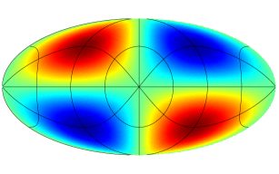
Figure 1: Initial configuration chosen for the temperature pattern.

We gratefully acknowledge the use of the Healpix software [75] in creating this and all the other all-sky maps shown hereafter.

Other choices are, of course, possible. A quadrupole with $m=0$ would produce a zonal pattern, and one with $m=2$ would be a sectoral mode [38]; these choices are discussed at some length in ref. [57]. One could also generate more complicated patterns by having an observer who is not at rest in the frame we are using, which would introduce an additional dipole anisotropy. We will not discuss this possibility further in this paper.

The simplest case is obviously that of Bianchi I, but this is nevertheless of some interest because a Universe of this type could in principle account for the presence of a low quadrupole [76, 77]. In this example the temperature pattern does not evolve at all with time, so one can simply treat the initial quadrupole as a free parameter. The polarization patterns arising in this model, which do not evolve with time either, are shown in Figure 2.

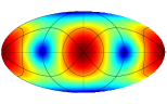
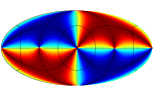
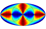
Figure 2: Polarization maps, i.e. polarization amplitude (left), Stokes parameter Q (middle) and U (right) of Bianchi type I.

We next turn our attention to Bianchi types V, VII_h and VII₀. These models have a single preferred axis of symmetry. The alignment of the shear eigenvectors relative to this preferred axis determines not only the dynamical evolution of the model through the field equations, but also the temperature and polarization pattern which, as we shall see, gets imprinted into the cosmic background radiation. Figure 3 shows (from bottom to top) the time evolution of the temperature pattern in these models. Note that, in Type V (left), the initial quadrupole retains its shape but gets focussed into a patch of decreasing size as time goes on. This is due to the effect of negative spatial curvature. In Bianchi Type VII₀ (right) the effect of rotation and shear is to twist the initial quadupole into a spiral shape that winds up increasingly as the system evolves. In the middle case, Bianchi Type VII_h we have a combination of the two cases either side: there is both a focussing and a twist. This case produces the most complicated temperature pattern.

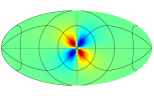
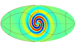
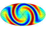
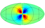
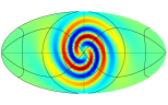
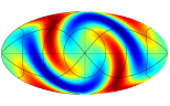
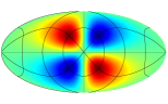
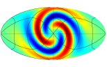
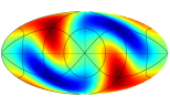
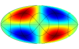
Figure 3: The time evolution of the temperature maps for Bianchi types V, VII_h and VII₀. Time increases from bottom to top.

In the following three figures we examine the polarization pattern produced in the models shown in Figure 2. First, in Figure 3, we have Bianchi V. These results show that while the polarization pattern alters with time in this case, its general orientation on the sky does not (as is the case with the temperature pattern). The implications of this for the production of cosmological B-mode polarization was discussed by ref. [55].

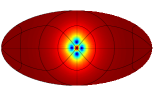
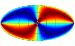
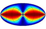
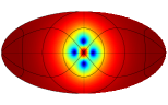
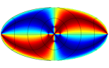
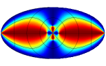
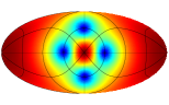
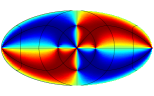
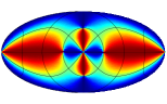
Figure 4: The time evolution of polarization maps for Bianchi V: degree of linear polarization (left); Stokes parameter Q (middle); and U(right). Time increases from bottom to top.

Figure 5 shows an example of Bianchi Type VII_h. Note the prodigious twisting of the polarized component of the radiation field, as well as a concentration of the degree of polarization defined by Equation (36). This case generically produces a large amount of mixing between $Q$ and $U$ during its time evolution.

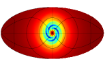
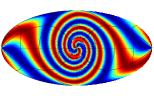
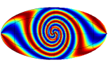
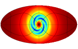
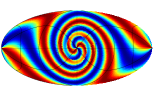
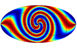
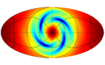
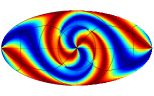
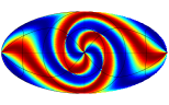
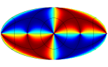
Figure 5: Same as Figure 4, but for Bianchi type VII_h.

Figure 6 shows, not unexpectedly, that Bianchi Type VII₀ produces a similar interweaving of the $Q$ and $U$ configurations, but without the focussing effect in the total polarized fraction.

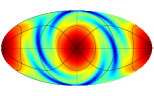
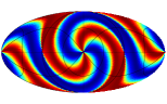
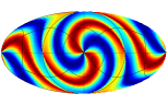
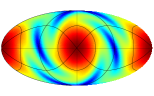
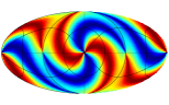
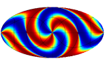
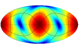
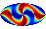
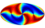
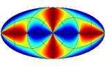
Figure 6: Same as Figure 4, but for Bianchi type VII₀.

Finally, for completeness we show results for Bianchi Type IX in Figure 7. This provides an interesting example of polarization behaviour because, in terms of polarization degree, the pattern does change at all with time but the Stokes maps $Q$ and $U$ do evolve. Bianchi Type IX models have positively curved spatial sections, and are equivalent in some sense to FRW models with the addition of circularly-polarized gravitational waves. These cause a rotation of the polarization angle but do not change the overall magnitude. The positive curvature does not allow for any focussing effects so the temperature pattern does not change with time either.

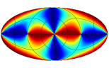
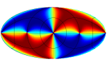
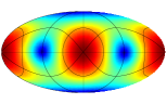
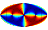
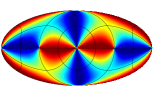
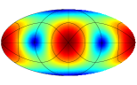
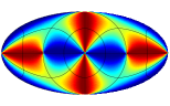
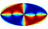
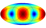
Figure 7: Same as Figure 4, but for Bianchi type IX.

6 Discussion and Conclusions

The goal of this work was to compute the temperature and polarization patterns produced in anisotropic relativistic cosmologies described by various Bianchi types. We focussed on those types that contain the standard homogeneous and isotropic FRW background as a limiting case. We constructed an appropriate description of the radiation field in terms of spin-0 and spin-2 components representing the unpolarized and polarized parts, respectively. We integrated the equations for the radiation field numerically, and presented illustrative examples here.

The basic point that emerges from this study is related to the physical origin of CMB polarization: radiation affected by Thomson scattering from an electron in a radiation field possessing a quadrupole anisotropy will inevitably be partially linearly polarized. In the context of standard cosmological models, the environment of different electrons varies owing to the presence of density inhomogeneities and a background of gravitational waves. These sources of variation are stochastic so the variations in the polarized component of the radiation field, though correlated with the temperature variations, are essentially incoherent. In Bianchi cosmologies, however, global homogeneity requires that each electron sees the same quadrupole. The polarized part of the radiation field is therefore coherent, and is in a fixed relationship to the temperature variation (once the model is specified).

We have exploited the formalism used to generate the examples shown here to produce an extensive test-bed of CMB temperature and polarization maps derived from Bianchi universe models of the types discussed in this paper. In future work we will analyse these maps using a variety of statistical measures of anisotropy. It is important to understand how standard statistical techniques, designed to be applied to stationary stochastic fluctuations, perform when applied to patterns which are neither stochastic nor stationary. Our Bianchi models, for example, yield patterns which have highly correlated spherical harmonic components in contrast to the case of a homogeneous Gaussian random field in which the harmonic modes are independent. It is important to understand how CMB fluctuations arising from Bianchi-type universes impact on orthodox analysis procedures and whether they produce characteristic signatures when analysed in this way, particularly in the presence of additional stochastic fluctuations. Higher-order statistics will be necessary to provide a full characterization of the coherent anisotropic fluctuations we have studied here. Moreover, present and future CMB experiments are largely aimed at improving the precision of polarization measurements in order to find evidence of a stochastic background of primordial gravitational waves. Techniques advocated to measure polarization pattern over the celestial sphere are therefore also generally tuned to detect signals of an incoherent nature. The presence of coherent signals in the CMB could be an indication of physics beyond the standard cosmological framework. This will hopefully lead us to better ways of searching for departures from the concordance cosmology using the next generation of datasets.

References

References

- [1] Bennett C L et al 2003 Astrophys. J. Supp. 148 1
- [2] Hinshaw G et al 2009 Astrophys. J. Supp. 180 225
- [3] Coles P 2005 Nature 433 248
- [4] Guth A H and Pi S Y 1982 Phys. Rev. Lett. 49 1110
- [5] Starobinskij A A 1982 Phys. Lett. B., 117 175
- [6] Bardeen J M, Steinhardt P J and Turner M S 1983 Phys. Rev. D. 28 679
- [7] Yadav A P S and Wandelt B D 2008 Phys. Rev. Lett. 100 181301
- [8] Vielva P, Martinez-Gonzalez E, Barreiro R B, Sanz J L and Cayon L 2004 Astrophys. J. 609 22
- [9] Cruz M, Martinez-Gonzalez E, Vielva P and Cayon L 2005 Mon. Not. R. astr. Soc. 356 29
- [10] Cruz M, Tucci M, Martinez-Gonzalez E and Vielva P 2006 Mon. Not. R. astr. Soc. 369 57
- [11] Cruz M, Cayon L, Martinez-Gonzalez E, Vielva P and Jin J 2007 Astrophys. J. 655, 11
- [12] Cruz M, Martinez-Gonzalez E, Vielva P, Diego J M, Hobson M and Turok N 2008 arXiv:0804.2904
- [13] Cayon L, Jin J and Treaster A 2005 Mon. Not. R. astr. Soc. 362 826
- [14] Naselsky P D, Christensen P R, Coles P, Verkhodanov O, Novikov D and Kim J 2009, arXiv/0712.1118
- [15] Schwarz D J, Starkman G D, Huterer D and Copi C J 2004 Phys. Rev. Lett. 93 221301
- [16] Copi C J, Huterer D and Starkman G D 2004 Phys. Rev. D. 70 043515
- [17] Katz G and Weeks J 2004 Phys. Rev. D. 70 063527
- [18] Land K and Magueijo J 2005 Mon. Not. R. astr. Soc. 357 994
- [19] Land K and Magueijo J 2005 Mon. Not. R. astr. Soc. 362 L16
- [20] Land K and Magueijo J 2005 Phys. Rev. D. 72 101302(R)
- [21] Land K and Magueijo J 2005 Phys. Rev. Lett. 95 071301
- [22] Land K and Magueijo J 2005 Mon. Not. R. astr. Soc. 362 838
- [23] Land K and Magueijo J 2007 Mon. Not. R. astr. Soc. 378 153
- [24] Copi C J, Huterer D, Schwarz D J and Starkman G D 2006 Mon. Not. R. astr. Soc. 367 79
- [25] Copi C J, Huterer D, Schwarz D J and Starkman G D 2007 Phys. Rev. D. 75 023507
- [26] Eriksen H K, Hansen F K, Banday A J, Górski K M and Lilje P B 2004 Astrophys. J. 605 14
- [27] Park C 2004 Mon. Not. R. astr. Soc. 349 313
- [28] Eriksen H K, Banday A J, Górski K M, Hansen F K and Lilje P B 2007, Astrophys. J. 660 L81
- [29] Hoftuft J, Eriksen H K, Banday A J, Górski K M, Hansen F K and Lilje P B 2009 Astrophys. J. Suppl. 699 985
- [30] Hansen F K, Banday A J, Górski K M, Eriksen H K and Lilje P B 2009 Astrophys. J. 704 1448
- [31] Hanson D and Lewis A 2009, arXiv: 0908.0963
- [32] Groeneboom N E, Ackerman L, Wehus I K and Eriksen H K 2009, arXiv: 0911.0150
- [33] Hanson D, Lewis A and Challinor A 2010, arXiv: 1003.0198
- [34] Zheng H and Bunn E F 2010, arXiv: 1003.5548
- [35] Chiang L-Y, Coles P, Naselsky P D and Olesen P 2007 J. Cosmol. Astropart. Phys. 01(2007)021
- [36] Chiang L-Y, Naselsky P D and Coles P 2007 Astrophys. J. 664 8
- [37] Francis C L and Peacock J A 2009, arXiv: 0909.2495
- [38] Short J and Coles P 2010 Mon. Not. R. astr. Soc. 401 2202
- [39] Grishchuk L P, Doroshkevich A G and Novikov I D 1968 Soviet Physics ZETP 55 2281
- [40] Ellis G F R and MacCallum M A H 1969 Commun. Math. Phys. 12 108
- [41] Collins C B and Hawking S W 1973 Mon. Not. R. astr. Soc. 162 307
- [42] Dautcourt G and Rose K 1978 Astr. Nachr. 299 13
- [43] Tolman B W and Matzner R A 1984 Proc. R. Soc. Lond. A 392 391
- [44] Matzner R A and Tolman B W 1982 Phys. Rev. D. 26 10
- [45] Tolman B W 1985 290 1
- [46] Barrow J D, Juszkiewicz R and Sonoda D H 1985 Mon. Not. R. astr. Soc. 213 917
- [47] Bunn E F, Ferreira P G and Silk J 1996 Phys. Rev. Lett. 77 2883
- [48] Kogut A, Hinshaw G and Banday A J 1997 Phys. Rev. D. 55 1901
- [49] Jaffe T R, Banday A J, Eriksen H K, Górski K M and Hansen F K 2005 Astrophys. J. 629 L1
- [50] Jaffe T R, Hervik S, Banday A J and Górski K M 2006 Astrophys. J. 644 701
- [51] McEwen J D, Hobson M P, Lasenby A N and Mortlock D J 2005 Mon. Not. R. astr. Soc. 369 1583
- [52] McEwen J D, Hobson M P, Lasenby A N and Mortlock D J 2006 Mon. Not. R. astr. Soc. 371 L50
- [53] Bridges M, McEwen J D, Lasenby A N and Hobson M P 2007 Mon. Not. R. astr. Soc. 377 1473
- [54] Sung R 2010 PhD thesis, Cardiff University
- [55] Sung R and Coles P 2009 Class. Quantum Grav. 26 172001
- [56] Pontzen A and Challinor A 2007 Mon. Not. R. astr. Soc. 380 1387
- [57] Pontzen A 2009 Phys. Rev. D. 79 103518
- [58] Page L et al 2007 Astrophys. J. Supp. 170 335
- [59] Kamionkowski M, Kosowsky A and Stebbins A 1997 Phys. Rev. D. 55 7368
- [60] Hu W and White M D 1997 Phys. Rev. D. 56 596
- [61] Frommert M and Enßlin T A 2010 Mon. Not. R. astr. Soc. 403 1739
- [62] Rees M J 1968 Astrophys. J. 153 L1
- [63] Nanos G P 1979 Astrophys. J. 232 341
- [64] Negroponte J and Silk J 1980 Phys. Rev. Lett. 44 1433
- [65] Basko M M and Polnarev A G 1980 Sov. Astr. 24 268
- [66] Polnarev A G 1985 Sov. Astron. 29 607
- [67] Frewin R A, Polnarev A G and Coles P Mon. Not. R. astr. Soc. 266 L21
- [68] Barrow J D 1986 in Gravitation in Astrophysics, eds Carter B and Hartle J B, Proceedings of NATO ASI Series B, 156 239
- [69] Coles P and Lucchin F 2002 Cosmology: The Origin and Evolution of Cosmic Structure, 2nd Edition, John Wiley & Sons
- [70] Ellis G F R 1967 J. Math. Phys. 8 1171
- [71] MacCallum M A H and Ellis G F R 1970 Commun. Math. Phys. 19 31
- [72] King A R and Ellis G F R 1973 Commun. Math. Phys. 31 209
- [73] Ellis G F R 2006 Gen. Rel. Grav. 38 1003
- [74] Kasner E 1921 Trans. Amer. Math. Soc. 43 217
- [75] Górski, K M, Hivon E, Banday A J, Wandelt B D, Hansen F K, Reinecke E M and Bartelmann M 2005 Astrophys. J. 622, 759
- [76] Campanelli L, Cea P and Tedesco L 2006 Phys. Rev. Lett. 97 209903
- [77] Campanelli L, Cea P and Tedesco L 2007 Phys. Rev. D. 76 063007