Signals of the cosmological reionization in the radio sky through C and O fine structure lines

Abstract

We study the excitation of fine structure levels of C i, C ii and O i by ultraviolet (UV) photons around strong UV sources which are also ionizing sources of the cosmological reionization at redshift of $\sim 10$. The evolutions of ionized regions around a point source are calculated by solving rate equations for non-equilibrium chemistry. Signals of UV photons through the fine structure lines are considered to be stronger at locations of more abundant chemical species of C i, C ii and O i. Such environments would be realized where strong fluxes of non-ionizing UV line photons available for the pumping up of fine structure levels exist, and simultaneously ionizing UV photons are effectively shielded by dense H i regions. Signals from H i regions of moderately large densities induced by redshifted UV photons emitted at the point sources are found to be dominantly large over those of others. We discuss the detectability of the signals, and show that signals from idealized environments will be possibly detected by radio observations with next-generation arrays to come after the Atacama Large Millimeter/submillimeter Array (ALMA).

1 Introduction

At the epoch of Big Bang Nucleosynthesis of cosmic temperature $T\ga 0.1$ MeV, light elements of ²H,^3,4He and ⁷Li are produced in abundances larger than $10^{-10}$ times that of hydrogen. As the temperature decreases, light elements recombine with electrons, and trace amounts of chemical molecules form during the Dark Ages between the recombination and the reionization of the universe (Vonlanthen et al., 2009). The universe is then considered to experience the reionization at temperature of $\sim 30$ K, i.e., cosmic redshift of $z\sim 10$ (Larson et al., 2010). Sources of the reionization are perhaps ultraviolet (UV) photons from quasi-stellar objects (QSOs), young galaxies and hypothetical low metallicity objects in the early universe, i.e., Population III stars, or some exotic energy injection processes triggered, for example, by the particle decay. If stars including Population III have contributed to the reionization, the metal enrichment in the universe would occur simultaneously. The reionization history as well as the metal enrichment of the universe is, however, not yet determined precisely. Many suggestions have been made for investigations of the cosmic reionization using atomic physics with future observations in radio frequency.

The first method is observations of intergalactic medium (IGM) through the redshifted 21 cm line of neutral hydrogen (Madau, Meiksin & Rees, 1997). The neutral gas regions could be quickly preheated to temperature larger than that of cosmic background radiation (CBR) in the presence of a strong flux of UV photons through the photoionization heating (e.g., Chen & Miralda-Escude, 2004). In such environments, the spin temperature determined by the population fractions of the upper and lower states of hyperfine levels is forced to deviate from the CBR temperature by level-mixing via Ly$\alpha$ photon scattering, i.e., Wouthuysen-Field effect (Wouthuysen, 1952; Field, 1958). There would be brief chances of observing them in absorption, and long chances in emission against the CBR. Future radio observations at meter wavelengths of IGM would produce plenty of information on the epoch, picture and sources of the reionization.

Although the 21 cm signal of the reionization of the universe is expected to be relatively strong, the strong contamination from Galactic and extragalactic foregrounds makes it difficult to observe the absolute signal over the whole sky except for fluctuations around it. Measurements of angular fluctuations in the H i signal are very difficult, while fluctuations in frequency would be easily separated and be detectable with future large arrays (Gnedin & Shaver, 2004). As for angular fluctuation, Di Matteo, Ciardi & Miniati (2004) have shown that angular fluctuations in 21 cm emission at $\theta\ga 1\arcmin$ can be detected if efficient subtraction of foreground sources is performed successfully. The 21 cm signal not by Wouthuysen-Field effect but by an effect of collision in earlier universe of higher densities has also been suggested to provide a valuable informations in the epoch when the spin temperature traced the gas kinetic temperature (Loeb & Zaldarriaga, 2004).

Long-lived metastable 2$s$ state of hydrogen has been studied, and signals of the reionization through 3 cm fine structure line (2$s_{1/2}\rightarrow 2p_{3/2}$) have been found to be undetectable with existing radio telescopes (Dijkstra et al., 2008). The reason is that a Ly$\beta$ photon which is the pumping source of the ground state can excite only one hydrogen atom into the 2$s$ state, while a Ly$\alpha$ photon can excite many atoms into the excited spin state. The signals through hyperfine transitions of D i, ³He ii (Deguchi & Watson, 1985) also exist. Sigurdson & Furlanetto (2006) have suggested a challenging possibility of determination of D/H abundance ratio by looking at hyperfine structure line at high redshift of both the H and D. Signals from IGMs and dense objects at high redshifts through the ³He hyperfine transition has been studied. Detailed physics and suggested observational plans were presented (McQuinn & Switzer, 2009), and the anticorrelation of H i 21 cm maps and ³He ii 3 cm maps was suggested (Bagla & Loeb, 2009).

The infrared fine structure lines of C i, C ii and O i (Bahcall & Wolf, 1968) play an important role in cooling of neutral regions (Hollenbach & Tielens, 1999). Astronomical observations of those lines provide rich information about physical conditions in observed objects (Kaufman et al., 1999). The signatures of existence of heavy chemical species like C and O through resonant scatterings with CBR imprinted on the CBR spectrum have been investigated (Basu, Hernández-Monteagudo & Sunyaev, 2004; Hernández-Monteagudo, Verde & Jimenez, 2006). With the Planck  spacecraft, the signatures can be searched for in the temperature anisotropy of CBR, and constraints on abundances of heavy species will be derived from the observations in reverse.

Idea of UV pumping through fine structure lines of metals during reionization as a way to distort the CMB during a reionization epoch has been suggested (Hernández-Monteagudo et al., 2007). They focused on the O i fine structure, and provided estimations for the order of magnitude of the distortion for different levels of UV fluxes. The angular power spectrum of the distortion introduced by the O i hosting regions at high redshift has subsequently been studied (Hernández-Monteagudo et al., 2008).

Observations of bright objects in radio frequency have been performed in search of emission lines of fine structures of heavy chemical species. The C ii 157$\mu$m line emissions of high redshift QSOs [J1148+5251 at $z=6.42$ (Maiolino et al., 2005), BR 1202-0725 at $z=4.7$ (Iono et al., 2006)] and a galaxy [BRI 0952-0115 at $z=4.43$ (Maiolino et al., 2009)] have been detected. Walter et al. (2009) observed the high redshift quasars (J1148+5251 at $z=6.42$) and derived an upper limit on a N ii 205$\mu$m line luminosity. The targets of these observations were, in fact, star-forming interstellar medium which emits through atomic fine structure lines. There are dense systems detected which absorb photon spectra of QSOs at fine structure transitions of C i, C ii and their physical conditions have been constrained (Silva & Viegas, 2002; Quast, Baade & Reimers, 2002; Reimers et al., 2005).

In this paper, we focus on cosmological signals of only UV sources without star forming activities through fine structure lines and their detectability. The structure of this paper is as follows. In Section 2, the pumping mechanism of fine structure levels and the dependence of the pumping efficiency as a redshift are shown. In Section 3, the model for calculation of reionization around a point source is introduced. In Section 4, the result of the calculation is presented. Intensities of signals of UV radiation from the source through fine structure lines are estimated, and the dependence of signals on the redshift is shown. We discuss the detectability of signals, and claim that signals may be detected by future radio measurements in $O(100-1000~{}{\rm GHz})$ range. In Section 5, we summarize our conclusions.

2 Ultraviolet Photon Pumping to C I, C II and O I Metastable States

2.1 Populations of Fine Structure Levels

2.1.1 Formulation

For a pair of two states, i.e., a stable and an unstable states, the spin temperature $T_{\rm S}$ is defined as

$$\frac{n_{\rm 1}}{n_{\rm 0}} = \frac{g_{1}}{g_{0}}\exp\left(-\frac{h\nu_{10}}{kT_{\rm S}}\right)$$ (1)

$$= \frac{g_{1}}{g_{0}}\exp\left(-\frac{T_{\ast}}{T_{\rm S}}\right),$$

where $n_{i}$ ($i=1$ for the upper state, $i=0$ for the lower) is the number density of the state $i$, $g_{i}=2S_{i}+1$ is the spin degrees of freedom of state $i$ with spin $S_{i}$, $h$ is the Planck’s constant, $\nu_{10}$ is the frequency corresponding to the transition from the state 1 to 0, $k$ is the Boltzmann’s constant. At the second equality, the temperature $T_{\ast}\equiv h\nu_{10}/k$ was defined. The spin temperature describes the ratio of occupation degree of the upper state to that of the lower.

For a group of three states, i.e., a ground state, a first excited state unstable to the decay into the ground state, and a second excited state unstable to the decay only into the first excited state, the spin temperature $T_{\rm S2}$ is defined as

$$\frac{n_{\rm 2}}{n_{\rm 1}} = \frac{g_{2}}{g_{1}}\exp\left(-\frac{T_{\ast 2}}{T_{\rm S2}}\right),$$ (2)

where the subscripts $i=1$ and $2$ are attached to physical values of the first and second excited states, respectively, the temperature $T_{\ast 2}\equiv h\nu_{21}/k$ is defined with the frequency for the transition from the state 2 to 1, i.e., $\nu_{21}$. Note that the spin temperatures for second excited states are defined using the number density of the $i=1$ and $2$ states, not $i=0$ and $2$ states.

Fine structure levels of C i, C ii and O i can be excited by continuum radiation at the frequency corresponding to the energy levels of excited states, UV radiation at the frequency corresponding to the energy levels of intermediate bound states, and by collisions. For two discrete fine structure energy levels denoted by 0 and 1, the rate equation for their population is written as

$$-\frac{dn_{0}}{dt}=\frac{dn_{1}}{dt} = A_{10}\left[\frac{c^{2}J_{\rm B}}{2h\nu^{3}}\frac{g_{1}}{g_{0}}n_{0}-\left(1+\frac{c^{2}J_{\rm B}}{2h\nu^{3}}\right)n_{1}\right]$$ (3)

$$+n_{0}P_{01}^{\rm UV}-n_{1}P_{10}^{\rm UV}+n_{0}C_{01}-n_{1}C_{10},$$

where $A_{10}$ is the Einstein $A$-coefficient of the $1\rightarrow 0$ transition, $\nu$ is the frequency of the transition and $C_{10}$ and $C_{01}$ are the collisional rates of the $1\rightarrow 0$ and $0\rightarrow 1$ transitions, respectively. $J_{\rm B}=\int\phi(\nu)I_{\nu}d\nu d\Omega/(4\pi)$ is the mean intensity of radiation, where $\phi(\nu)$ is the line profile function and $I_{\nu}$ is the specific intensity at the transition frequency. The rates of excitation and deexcitation by UV photons, i.e., $P_{01}^{\rm UV}$ and $P_{01}^{\rm UV}$ are given by

$$P_{01}^{\rm UV}=\sum_{j}\left(\frac{c^{2}}{2h\nu_{j0}^{3}}\right)\left(\frac{A_{j0}J_{j0}g_{j}}{g_{0}}\right)\frac{A_{j1}}{\sum_{i}A_{ji}},$$ (4)

$$P_{10}^{\rm UV}=\sum_{j}\left(\frac{c^{2}}{2h\nu_{j1}^{3}}\right)\left(\frac{A_{j1}J_{j1}g_{j}}{g_{1}}\right)\frac{A_{j0}}{\sum_{i}A_{ji}},$$ (5)

where $j$ indicates excited levels above the fine structure multiplets and $i$ is either 0 or 1. There are several or more excited levels of C i, C ii and O i where transitions from the ground state fine structure levels by electric dipole interaction are allowed. Although many lines could contribute to populating excited states of fine structures, we treat only transitions corresponding to the lowest energies for respective species for the moment. All of the permitted lines are considered in Section 4.2.2.

Figure 1 shows the transitions from the ground state fine structures to the lowest energy levels which is connected to the fine structures through strong electric dipole transitions. Numbers attached to lines are relative strengths of spontaneous emission rates $A$.

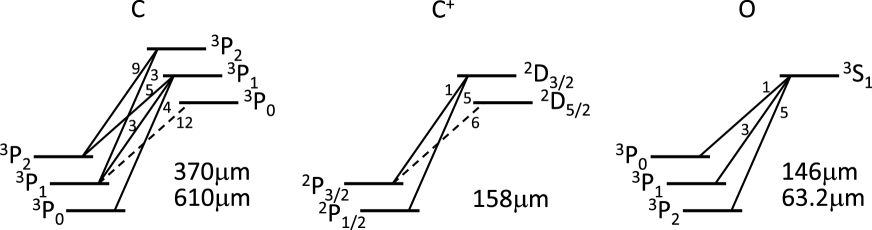
Figure 1: Diagrams for ultraviolet permitted transitions which mix the ground state fine structures (solid lines) and do not (dashed lines). The attached numbers are relative strengths of spontaneous emission rates $A$.

The spin temperature in the steady state is derived from equation (3). We assumed the Planck distribution of the mean intensity $J_{\rm B}$ with the temperature of cosmic background radiation (CBR), i.e., $T_{\rm CBR}=2.725(1+z)$ K (Mather et al., 1999) with the redshift $z$. In addition, the thermal energy distribution of gas is assumed. The collisional transition rates are then given by

$$C_{ij}=n_{\rm target}\gamma_{ij}(T_{\rm gas}),$$ (6)

where $n_{\rm target}$ is the number density of target species and $\gamma_{ij}$ is the collisional (de)excitation coefficient as a function of the gas temperature, i.e., $T_{\rm gas}$.

For the C ii two level states, the spin temperature is

$$T_{\rm S}=-T_{\ast}\left\{\ln\left[\frac{{\rm e}^{-T_{\ast}/T_{\rm CBR}}+y_{\rm L}{\rm e}^{-T_{\ast}/T_{\rm UV}}+y_{\rm C}{\rm e}^{-T_{\ast}/T_{\rm gas}}}{1+y_{\rm L}+y_{\rm C}}\right]\right\}^{-1},\\$$ (7)

where $T_{\rm UV}$ is given by the relation

$$\frac{P_{10}^{\rm UV}}{P_{01}^{\rm UV}}=\frac{g_{0}}{g_{1}}\exp\left(\frac{T_{\ast}}{T_{\rm UV}}\right),$$ (8)

(Field, 1958; Deguchi & Watson, 1985), The temperature $T_{\rm gas}$ satisfies

$$\frac{P_{10}^{\rm C}}{P_{01}^{\rm C}}=\frac{g_{0}}{g_{1}}\exp\left(\frac{T_{\ast}}{T_{\rm gas}}\right),$$ (9)

and

$$y_{\rm L}=\frac{P_{10}^{\rm UV}}{A_{10}}\left[1-\exp(-T_{\ast}/T_{\rm CBR})\right],$$ (10)

$$y_{\rm C}=\frac{P_{10}^{\rm C}}{A_{10}}\left[1-\exp(-T_{\ast}/T_{\rm CBR})\right]$$ (11)

were defined.

For three level states, the equations describing the balance between production and destruction of the first and second excited states are given by

$$n_{0}P_{01}+n_{2}P_{21}=n_{1}\left(P_{10}+P_{12}\right),$$ (12)

$$n_{0}P_{02}+n_{1}P_{12}=n_{2}\left(P_{20}+P_{21}\right),$$ (13)

where $P_{ij}$ includes transitions $i\rightarrow j$ by all of the CBR continuum, UV radiation and particle collision. The sum of the above two equations is equal to the balance equation for the ground state. These equations are solved for number fractions of the energy states, that is

$$\frac{n_{1}}{n_{0}}=\frac{P_{01}P_{20}+P_{21}P_{02}+P_{01}P_{21}}{P_{10}P_{20}+P_{12}P_{20}+P_{10}P_{21}},$$ (14)

$$\frac{n_{2}}{n_{0}}=\frac{P_{10}P_{02}+P_{12}P_{02}+P_{01}P_{12}}{P_{10}P_{20}+P_{12}P_{20}+P_{10}P_{21}}.$$ (15)

Spin temperatures, i.e., $T_{\rm S}$ and $T_{\rm S2}$ of the first and second excited states are calculated using equations (1) and (2).

Table 1 shows data on the fine structure and UV transitions taken from Ralchenko et al. (2008) as well as data on the collisional deexcitaion coefficients taken from Hollenbach & McKee (1989). As for C i the difference between energy levels of ${}^{3}P_{2}$ and ${}^{3}P_{1}$ in the excited states higher than that of the ground state by $\sim 6\times 10^{4}$ cm^-1 is $40.51$ cm^-1 (Ralchenko et al., 2008).

Table 1: Fine structure and UV transitions

	Fine structure transition				UV transition
Species	State	$\nu$ (GHz)	$A$ (s-1)	$\gamma_{ij}^{\rm H}$ (cm3 s-1)	State	$\nu$ (cm-1)	$A$ (s-1)
C i	3P${}_{1}-^{3}$P0	492	$7.88\times 10^{-8}$	$1.6\times 10^{-10}T_{2}^{0.14}$	3P${}_{1}-^{3}$P0	$6.035\times 10^{4}$	$1.13\times 10^{8}$
	3P${}_{2}-^{3}$P0	1301		$9.2\times 10^{-11}T_{2}^{0.26}$	3P${}_{1}-^{3}$P1		$8.64\times 10^{7}$
	3P${}_{2}-^{3}$P1	809	$2.65\times 10^{-7}$	$2.9\times 10^{-10}T_{2}^{0.26}$	3P${}_{1}-^{3}$P2		$1.44\times 10^{8}$
					3P${}_{2}-^{3}$P1		$8.58\times 10^{7}$
					3P${}_{2}-^{3}$P2		$2.52\times 10^{8}$
C ii	2P${}_{3/2}-^{2}$P1/2	1901	$2.30\times 10^{-6}$	$8.0\times 10^{-10}T_{2}^{0.07}$	2D${}_{3/2}-^{2}$P1/2	$7.493\times 10^{4}$	$2.37\times 10^{8}$
					2D${}_{3/2}-^{2}$P3/2		$4.74\times 10^{7}$
O i	3P${}_{1}-^{3}$P2	4745	$8.91\times 10^{-5}$	$9.2\times 10^{-11}T_{2}^{0.67}$	3S${}_{1}-^{3}$P2	$7.679\times 10^{4}$	$3.41\times 10^{8}$
	3P${}_{0}-^{3}$P2	6805		$4.3\times 10^{-11}T_{2}^{0.80}$	3S${}_{1}-^{3}$P1		$2.03\times 10^{8}$
	3P${}_{0}-^{3}$P1	2060	$1.75\times 10^{-5}$	$1.1\times 10^{-10}T_{2}^{0.44}$	3S${}_{1}-^{3}$P0		$6.76\times 10^{7}$

2.1.2 Effects of UV pumping and Collisions

We compare effects of UV pumping and collisions on populations of fine structure levels. The effects are not so large as that of CBR if the physical condition which is considered is not dense and not very near to extremely luminous objects. First, we define $f_{ij}$ as the number ratio

$$f_{ij}(y_{\rm L},T_{\rm UV},y_{\rm C},T_{\rm gas},T_{\rm CBR})\equiv n_{i}/n_{j}.$$ (16)

Using equation (7) we can describe the deviation of $f_{10}$ for a two level system under a UV source and/or a collisional environment from that for no such effects by the first order Taylor expansions in $y_{\rm L}$ and $y_{\rm C}$, i.e.,

$$\frac{\Delta f_{10}(y_{\rm L},T_{\rm UV},y_{\rm C},T_{\rm gas},T_{\rm CBR})}{f_{10}(0,^{\forall}T_{\rm UV},0,^{\forall}T_{\rm gas},T_{\rm CBR})}\equiv\frac{f_{10}(y_{\rm L},T_{\rm UV},y_{\rm C},T_{\rm gas},T_{\rm CBR})}{f_{10}(0,^{\forall}T_{\rm UV},0,^{\forall}T_{\rm gas},T_{\rm CBR})}-1$$

$$=y_{\rm L}\left[\exp\left(-\frac{T_{\ast}}{T_{\rm UV}}+\frac{T_{\ast}}{T_{\rm CBR}}\right)-1\right]$$

$$+y_{\rm C}\left[\exp\left(-\frac{T_{\ast}}{T_{\rm gas}}+\frac{T_{\ast}}{T_{\rm CBR}}\right)-1\right]$$

$$\equiv(\Delta f_{10}/f_{10})_{\rm L}+(\Delta f_{10}/f_{10})_{\rm C}.$$ (17)

The first and second terms in the left hand side are contributions of UV pumping and collisions, respectively. The explicit expression for $f_{10}$ value is

$$f_{10}(y_{\rm L},T_{\rm UV},y_{\rm C},T_{\rm gas},T_{\rm CBR})$$ (18)

$$= \frac{g_{1}}{g_{0}}\left[{\rm e}^{-T_{\ast}/T_{\rm CBR}}+y_{\rm L}\left({\rm e}^{-T_{\ast}/T_{\rm UV}}-{\rm e}^{-T_{\ast}/T_{\rm CBR}}\right)\right.$$

$$\hskip 15.00002pt\left.+y_{\rm C}\left({\rm e}^{-T_{\ast}/T_{\rm gas}}-{\rm e}^{-T_{\ast}/T_{\rm CBR}}\right)\right].$$

Figure 2 shows contours of $(\Delta f_{10}/f_{10})_{\rm L}$ (upper panel) on the parameter plane of UV color temperature $T_{\rm UV}$ and scattering rate $P_{\nu}$ for the UV transition ${}^{2}P_{3/2}\rightarrow^{2}D_{3/2}$, and also contours of $(\Delta f_{10}/f_{10})_{\rm C}$ on the parameter plane of the gas temperature $T_{\rm gas}$ and the number density of H i $n_{\rm H_{I}}$ (lower panel). For this figure, the redshift was assumed to be $z=10$, and the target in collisional (de)excitation was assumed to be H i. Solid and dashed lines correspond to positive and negative values for indicated amplitudes, respectively. Because of $T_{\rm UV}\gg T_{\ast}$ the effect of UV pumping is not sensitive to $T_{\rm UV}$ [cf. equation (17)]. $(\Delta f_{10}/f_{10})_{\rm C}$ is positive in the parameter region of $T_{\rm gas}>T_{\rm CBR}$ while it is negative in the parameter region of $T_{\rm gas}<T_{\rm CBR}$ [cf. equation (17)].

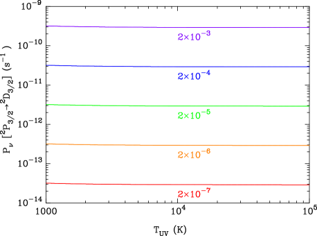
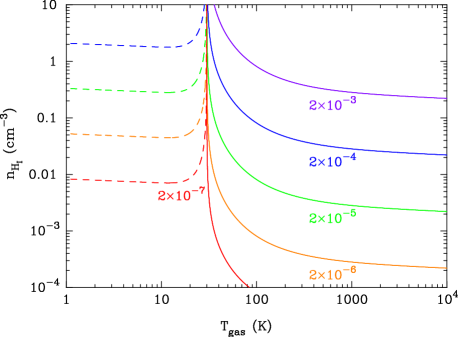
Figure 2: Contours of deviations in number ratio $n_{1}/n_{0}$ from the values for only CBR contribution. The upper panel shows the contribution of UV pumping on the parameter plane of UV color temperature $T_{\rm UV}$ and scattering rate $P_{\nu}$ for the UV transition ${}^{2}P_{3/2}\rightarrow^{2}D_{3/2}$. The lower panel shows the contribution of collisions on the parameter plane of the gas temperature $T_{\rm gas}$ and the number density of H i $n_{\rm H_{I}}$. Solid and dashed lines correspond to positive and negative values for indicated amplitudes, respectively.

Figure 3 shows contours for C i fine structure lines of $(\Delta f_{10}/f_{10})_{\rm L}$ (solid lines) and $(\Delta f_{21}/f_{21})_{\rm L}$ (dotted) (upper panel) on the parameter plane of $T_{\rm UV}$ and $P_{\nu}$ for the UV transition ${}^{3}P_{0}$ (ground state) $\rightarrow^{3}P_{1}$, and also contours of $(\Delta f_{10}/f_{10})_{\rm C}$ [solid (for positive values) and dashed lines (for negative values)] and $(\Delta f_{21}/f_{21})_{\rm C}$ [dotted (positive) and dot-dashed lines (negative)] on the parameter plane of $T_{\rm gas}$ and $n_{\rm H_{I}}$ (lower panel). The redshift was assumed to be $z=10$, and the target in collisional (de)excitation was assumed to be H i.

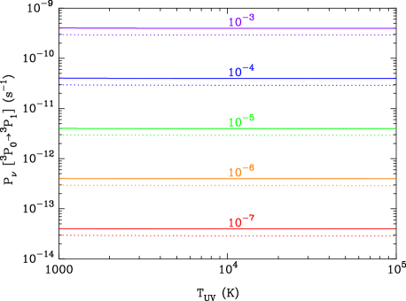
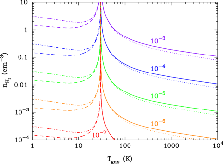
Figure 3: Same as in Fig 2 but for $n_{1}/n_{0}$ [solid (for positive values) and dashed lines (for negative values)] and $n_{2}/n_{1}$ [dotted (positive) and dot-dashed lines (negative)] of C i. The upper panel shows the contribution of UV pumping on the parameter plane of $T_{\rm UV}$ and $P_{\nu}$ for the UV transition ${}^{3}P_{0}$ (ground state) $\rightarrow^{3}P_{1}$. The lower panel shows the contribution of collisions on the plane of $T_{\rm gas}$ and $n_{\rm H_{I}}$.

Figure 4 shows contours for O i fine structure lines of $(\Delta f_{10}/f_{10})_{\rm L}$ (solid lines) and $(\Delta f_{21}/f_{21})_{\rm L}$ (dotted) (upper panel) on the parameter plane of $T_{\rm UV}$ and $P_{\nu}$ for the UV transition ${}^{3}P_{2}\rightarrow^{3}S_{1}$, and also contours of $(\Delta f_{10}/f_{10})_{\rm C}$ [solid (for positive values) and dashed lines (for negative values)] and $(\Delta f_{21}/f_{21})_{\rm C}$ [dotted (positive) and dot-dashed lines (negative)] on the parameter plane of $T_{\rm gas}$ and $n_{\rm H_{I}}$ (lower panel). The redshift was assumed to be $z=10$, and the target in collisional (de)excitation was assumed to be H i.

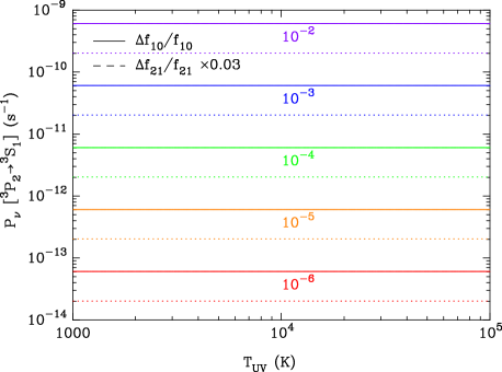
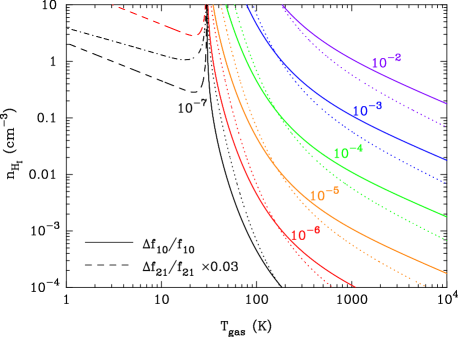
Figure 4: Same as in Fig 3 but for O i. The upper panel shows the contribution of UV pumping on the parameter plane of $T_{\rm UV}$ and $P_{\nu}$ for the UV transition ${}^{3}P_{2}\rightarrow^{3}S_{1}$. The lower panel shows the contribution of collisions on the plane of $T_{\rm gas}$ and $n_{\rm H_{I}}$.

From Figs. 2, 3 and 4, it is found that under environments of intense UV fluxes and relatively low densities and low gas temperatures considered in this study, the effect of UV pumping is typically larger than that of collisions. We, therefore, neglect the effect of collisions on the population of fine structures in what follows.

2.2 Intensities of Redshifted Fine Structure Radiation

We estimate a signal from a region including abundant C i or C ii, or O i of angular size on the sky that is larger than a beam width, and of radial velocity range that is larger than the bandwidth. For a fine structure line of frequency $\nu_{0}$, a intergalactic optical depth at frequency $\nu_{0}/(1+z)$ along the line of sight is (Hernández-Monteagudo et al., 2007)

$$\tau=\frac{A_{ij}\lambda_{ij}^{3}n_{A_{N}}(z)\left(g_{i}f_{j}/g_{j}-f_{i}\right)}{8\pi H_{0}\sqrt[]{\mathstrut\Omega_{\rm m}(1+z)^{3}+1-\Omega_{\rm m}}},$$ (19)

where $(i,j)=(1,0)$ or $(2,1)$, $\lambda_{ij}$ is the wavelength for transition $i\rightarrow j$, $n_{A_{N}}(z)$ is the number density of chemical species $A_{N}$ (C i, C ii or O i) at redshift $z$, $f_{i}=n_{i}/\left(\sum_{i}n_{i}\right)$ is the population fraction of energy state $i$, $H_{0}=71.9^{+2.6}_{-2.7}$ km s^-1 Mpc^-1 (Dunkley et al., 2009) is the Hubble constant, $\Omega_{\rm m}$ is the energy density parameters of matter (e.g., Madau et al., 1997; Padmanabhan, 1993). The optical depth in the homogeneous universe is typically much less than unity. In the optically thin case, the intensity of the signal $\Delta I_{\nu}$ with respect to that of the CBR radiation $B_{\nu}(T_{\rm CBR})$ is

$$\frac{\Delta I_{\nu}}{B_{\nu}(T_{\rm CBR})}=\left[\frac{\exp(T_{\ast}/T_{\rm CBR})-1}{\exp(T_{\ast}/T_{S})-1}-1\right]\tau,$$ (20)

which is identical to equation (9) in Hernández-Monteagudo et al. (2007) under the assumption that the background radiation field is that of thermal CBR. In this study, we investigate signals of the UV continuum radiation left on the radio background via excitations of fine structure lines. The UV source is assumed to have a power law luminosity spectrum, i.e., $L_{\nu}\propto\nu^{-\alpha_{S}}$. When the UV photon scattering occurs close to the emission redshift, the total scattering rate $P_{\nu}$ for a point source is given by

$$P_{\nu} = \frac{\lambda_{lu}^{2}}{8\pi}\frac{g_{u}}{g_{l}}A_{ul}\frac{L_{\nu}/(h\nu)}{4\pi r^{2}}$$ (21)

$$= 7.6\times 10^{-9}~{}{\rm s}^{-1}~{}\frac{g_{u}}{g_{l}}\left(\frac{\lambda_{lu}}{\lambda_{\alpha}}\right)^{\alpha_{S}+3}\left(\frac{A_{ul}}{A_{\alpha}}\right)\frac{\left(\nu L_{\nu}\right)_{\alpha,47}}{(r_{\rm Mpc}/0.1)^{2}},$$

(cf. Madau et al., 1997) where the subscripts $l$ and $u$ mean the low energy state of fine structure and the upper energy state to which the transition from the state $l$ is allowed, respectively, $r$ is the proper distance between the emission and scattering. In the second equality, $\lambda_{\alpha}=1.215\times 10^{-5}$ cm is the wavelength for Ly$\alpha$ transition of H i, $A_{\alpha}=6.265\times 10^{8}$ s^-1 is the spontaneous emission rate for Ly$\alpha$, $\left(\nu L_{\nu}\right)_{\alpha,47}$ is the product of the luminosity of the point source and the frequency of photon at Ly$\alpha$ frequency in units of $10^{47}$ ergs s^-1, and $r_{\rm Mpc}$ is the distance $r$ in Mpc.

Figure 5 shows signals through fine structure lines relative to corresponding cosmic background radiation as a function of the redshift under the following assumptions: The universe is homogeneous, and the number density of hydrogen is $n_{\rm H}=1.9\times 10^{-7}$ cm${}^{-3}(1+z)^{3}$. The abundances of C and O in the universe at redshift $z$ are $y_{\rm C}=1.4\times 10^{-4}$ and $y_{\rm O}=3.2\times 10^{-4}$, respectively, which correspond to local ISM values (Maiolino et al., 2005). The elements (C and O) are assumed to be completely in the chemical species (C i, C ii and O i), i.e., $n_{\rm C_{I}}=n_{\rm H}y_{\rm C}$, $n_{\rm C_{II}}=n_{\rm H}y_{\rm C}$ and $n_{\rm O_{I}}=n_{\rm H}y_{\rm O}$, respectively. A QSO of luminosity of $L_{\nu}=4.1\times 10^{31}(\nu/\nu_{\alpha})^{-\alpha_{S}}$ ergs s^-1 Hz^-1 [corresponding to $\left(\nu L_{\nu}\right)_{\alpha,47}=1$] with $\alpha_{S}=1/2$ (solid lines), $\alpha_{S}=3/2$ (dashed) and $\alpha_{S}=5/2$ (dotted) is assumed to shine at a distance of 1 Mpc ($r_{\rm Mpc}=1$). A decrease in flux of UV photons associated with continuous scattering with C i, C ii and O i during their propagation is not considered. This effect is found very important in Section 4 below. In drawing this figure we confirmed that the spin temperature of O i 228 K line calculated with equations given in Sec 2.1 is exactly equal to that described by an approximate equation (7) of Hernández-Monteagudo et al. (2007).

At high redshift of $z\ga 10$, all signals are small at the distance of $r_{\rm Mpc}=1$. As the redshift decreases, spin temperatures become smaller with the CBR temperature decreasing by redshift. Optical depths decrease since the number density of particles decrease with the cosmic expansion [see equation (19)]. Since the number density of the CBR is smaller and its energy is lower at low redshift, the UV pumping effect gets relatively dominant over the CBR effect below some critical redshifts for respective fine structure lines. Spin temperatures then decouple from the CBR temperature at the critical redshifts in the present setting of fixed radius. Since the CBR temperature at low redshift is less than the line temperatures, i.e., ($T_{\ast}>T_{\rm CBR}$), the decoupling of the spin temperature ($T_{\rm S}>T_{\rm CBR}$) leads to the large difference of line intensity from that of CBR. The factor in the angle bracket in the right hand side of equation (20) is, therefore, large. The signal to CBR ratios are enhanced at low redshift for these reasons.

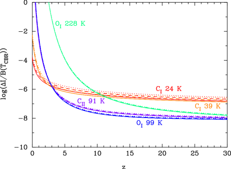
Figure 5: Signals through fine structure lines in the homogeneous universe relative to corresponding cosmic background radiation as a function of the redshift. A QSO of luminosity of $L_{\nu}=4.1\times 10^{31}(\nu/\nu_{\alpha})^{-\alpha_{S}}$ ergs s^-1 Hz^-1 with $\alpha_{S}=1/2$ (solid lines), $\alpha_{S}=3/2$ (dashed) and $\alpha_{S}=5/2$ (dotted) is assumed to shine at a distance of 1 Mpc. The respective lines are derived under the assumption that the elements (C and O) are completely in the chemical species (C i, C ii and O i), and therefore maximum values.

2.3 UV Color Temperature

We mention an important point on the UV color temperature, for example, of the ground state of C i.

In a time scale for UV photons to scatter C i particles by UV pumping, i.e., the mean free time, the color temperature of the UV photon around the line center relaxes to the kinetic temperature of the gas (i.e., C i here) (Field, 1959; Rybicki & dell’Antonio, 1994). The mean free time of a line center photon is $\tau^{\rm line}=1/(n_{\rm C_{I}}\sigma_{\nu}^{\rm C})$ with $\sigma_{\nu}^{\rm C}$ the UV line absorption cross section at the line center. The line absorption cross section is

$$\sigma_{\nu}=\frac{\lambda_{ul}^{2}}{8\pi}\frac{g_{u}}{g_{l}}A_{ul}\phi(\nu).$$ (22)

Neglecting the microturbulence and the very small effect of natural broadening, the line center cross section is

$$\sigma_{\nu}^{\rm C}=\frac{\lambda_{ul}^{2}}{8\pi}\frac{g_{u}}{g_{l}}A_{ul}\frac{1}{\sqrt[]{\mathstrut\pi}\Delta\nu_{\rm D}},$$ (23)

where

$$\Delta\nu_{\rm D}=\frac{\nu_{0}}{c}\sqrt[]{\mathstrut\frac{2kT_{\rm gas}}{m}}$$ (24)

is the Doppler width with $m$ the mass of an atom (Rybicki & Lightman, 1979).

Using this equation and $n_{\rm C{\sc\,I}}=n_{\rm H}\delta_{\rm b}y_{\rm C}$, the mean free time is found to be

$$\tau^{\rm line}=4.2~{}{\rm yr}~{}T_{\rm gas,K}^{1/2}\left(\frac{1+z}{10}\right)^{-3}\delta_{\rm b}^{-1}\left(\frac{y_{\rm C}}{1.4\times 10^{-4}}\right)^{-1}.$$ (25)

where $T_{\rm gas,K}$ is the gas temperature in units of K, $\delta_{\rm b}$ is the local density excess in units of the universal average value of baryonic matter. The color temperature around the line frequency, therefore, could approach to the gas temperature depending on the temperature of the gas, redshift, density excess, and the abundance of the scattered species. Since the Doppler width $\Delta\nu_{\rm D}=2.2\times 10^{8}{\rm s}^{-1}T_{\rm gas,K}^{1/2}$ is much smaller than the frequencies corresponding to the hyperfine transitions of $\nu=O(10^{11}-10^{12}{\rm s}^{-1})$, line photons of different frequencies are completely distinguished at scattering processes with C and O. In other words, a photon with frequency for one line transition can not induce scatterings corresponding to other transitions. Furthermore, strong lines which enable changes in photon energy do not exist around the frequencies of the UV pumping lines. The color temperature is, therefore, given by an original color temperature of the source $T_{\rm UV}=h\nu_{\rm line}/[k(3+\alpha_{S})]$ before relaxing to the spin temperature by scattering with C or O. This situation is completely different from the case of the Ly$\alpha$ pumping in which Ly$\alpha$ photon can mix the hyperfine levels of the H i ground state many times (Madau et al., 1997).

3 Numerical Calculation of 1D Hydrodynamics

We calculated a hydrodynamics coupled to a chemical reaction network assuming the spherical symmetry of space in order to show an example of geometric structure of ionized region.

3.1 Hydrodynamics

3.1.1 Fluid Equations

The hydrodynamic equations to be solved in this study are as follows:

$$\frac{\partial\rho}{\partial t}+{\bf\nabla}\cdot\left(\rho{\bf v}\right)=0,$$ (26)

$$\frac{\partial{\bf v}}{\partial t}+\left({\bf v}\cdot{\bf\nabla}\right){\bf v}=-\frac{{\bf\nabla}p}{\rho}-{\bf\nabla}\Phi,$$ (27)

$$\frac{\partial\left(\rho E\right)}{\partial t}+{\bf\nabla}\cdot\left[\left(\rho E+p\right){\bf v}\right]=S,$$ (28)

where $t$ and ${\bf r}$ are the time and the position, respectively, $\rho$, ${\bf v}$, $p$ and $\Phi$ are the density, velocity, pressure and gravitational potential as a function of $t$ and ${\bf r}$, respectively, $E\equiv v^{2}/2+\epsilon$ is the fluid energy per unit mass with $\epsilon=p/\left[(\gamma-1)\rho\right]$ the internal energy and $\gamma$ the ratio of specific heat, $S=\Gamma-\Lambda$ is the energy gain with $\Gamma$ and $\Lambda$ the heating and cooling terms, respectively. The ratio of specific heat is fixed to be $\gamma=5/3$ in this study.

We here introduce the comoving coordinates (Shandarin, 1980; Shapiro & Struck-Marcell, 1985) using comoving variables to describe deviations of the fluid quantities from those of the expanding homogeneous universe. New variable denoted by primes are

$$dt^{\prime}=a^{-2}dt,$$ (29)

$${\bf r^{\prime}}=a^{-1}{\bf r},$$ (30)

$$\rho^{\prime}=a^{3}\rho,$$ (31)

$${\bf v^{\prime}}=a\left[{\bf v}-H(t){\bf r}\right],$$ (32)

$$p^{\prime}=a^{5}p,$$ (33)

$$\epsilon^{\prime}=a^{2}\epsilon=p^{\prime}/\left[\left(\gamma-1\right)\rho^{\prime}\right],$$ (34)

$$S^{\prime}=a^{7}S,$$ (35)

where $a(t)=1/(1+z)$ is the scale factor of the universe with $z$ the redshift, and $H(t)=\dot{a}/a$ is the Hubble expansion rate. The peculiar gravitational potential is assumed to be negligible, and only the potential in a homogeneous isotropically expanding universe is considered here, i.e.,

$$\Phi(t,r)=\frac{2\pi G\bar{\rho}(t)r^{2}}{3},$$ (36)

where $G$ is the gravitational constant, and $\bar{\rho}(t)$ is the mean density at time $t$.

We assume that the cosmic expansion is described by $\Lambda$CDM model. The cosmological parameters are taken from a fit to the Wilkinson Microwave Anisotropy Probe (WMAP) 5 year data (Model $\Lambda$CDM+SZ+lens). (Dunkley et al., 2009) The energy density parameters of baryon, matter and dark energy are $\Omega_{\rm b}=0.0441\pm 0.0030$, $\Omega_{\rm m}=0.258\pm 0.030$ and $\Omega_{\Lambda}=0.742\pm 0.0030$ respectively. In this study we concentrate on the early epoch of the universe, i.e., $z>1$. The model, therefore, is effectively the CDM dominated universe.

Under the assumption of the CDM dominated universe and of the ratio of specific heat $\gamma=5/3$, the fluid equations are transformed into the following ones:

$$\frac{\partial\rho^{\prime}}{\partial t^{\prime}}+{\bf\nabla^{\prime}}\cdot\left(\rho^{\prime}{\bf v^{\prime}}\right)=0,$$ (37)

$$\frac{\partial\left(\rho^{\prime}{\bf v^{\prime}}\right)}{\partial t^{\prime}}+{\bf\nabla^{\prime}}\left(\rho^{\prime}{v^{\prime}}^{2}+p^{\prime}\right)=0,$$ (38)

$$\frac{\partial}{\partial t^{\prime}}\left(\rho^{\prime}E^{\prime}\right)+{\bf\nabla^{\prime}}\cdot\left[\rho^{\prime}\left(E^{\prime}+\frac{p^{\prime}}{\rho^{\prime}}\right){\bf v^{\prime}}\right]=S^{\prime}.\\$$

where $E^{\prime}\equiv{v^{\prime}}^{2}/2+\epsilon^{\prime}$ was defined. These equations do not include the cosmic expansion explicitly . They are solved simultaneously with the time evolution of the scale factor $a(t)$.

3.1.2 Heating and Cooling Rates

As a heating term, the photoionization is included. The heating rate from kinetic energy of photoelectrons and protons produced by photoionization is given by

$$\Gamma = \sum_{i={\rm H_{I}},{\rm He_{I}},{\rm He_{II}}}n_{i}\times$$ (39)

$$\int_{E_{{\rm th},i}}^{\infty}dE_{\gamma}~{}\left(E_{\gamma}-E_{{\rm th},i}\right)n_{\gamma}(E_{\gamma})\sigma^{\rm ion}_{i}(E_{\gamma})c,$$

where $E_{\gamma}$ is the energy of nonthermal photon, $E_{{\rm th},i}$ is the threshold energy for photoionization of species $i$, $n_{\gamma}(E_{\gamma})$ is the energy spectrum of the photon number density as a function of time $t$ and position $r$, $\sigma^{\rm ion}_{i}(E_{\gamma})$ is the photoionization cross section, and $c$ is the light speed. The production of secondary electrons at the photoionization of H and He is followed, and additional energy inputs by these electrons are taken into account in the estimation of the heating rate. For the photoionization cross sections we used the FORTRAN subroutine phfit2 by D. A. Verner. We adopted the fitted functions from Shull & van Steenberg (1985) for heat generation fractions associated with secondary electrons produced by the H i and He i photoionization.

As cooling terms, radiative coolings due to collisional recombination, excitation, ionization and free-free transitions as well as the Compton cooling off the CBR are included. We adopt the cooling rates for Case B (optically thick case) recombinations of H ii and He iii by Hummer (1994) and that of He ii by Hummer & Storey (1998). The cooling from the dielectronic recombination of He ii is also included with its rate taken from Shapiro & Kang (1987). The cooling rates for the collisional line excitation are calculated using the excitation rates given in Sobelman, Vainshtein & Yukov (1981) for excitations of H i, He i and He ii from the ground states of main quantum number $n=1$ to excited states of $n=2,3$ and 4.

Below $10^{4}$ K, metastable transitions or fine structure transitions of dominant metal species contribute to the cooling. We, therefore, include important line transitions of C i, C ii and O i (Hollenbach & McKee, 1989). The cooling rate for fine structure transitions of species $i$ is given by

$$\Lambda_{\rm fs} = n_{i}\sum_{l<u}f_{l}\frac{g_{u}}{g_{l}}\left[\exp(-E_{ul}/T_{\rm gas})-\exp(-E_{ul}/T_{\rm CBR})\right]$$ (40)

$$\times\sum_{j={\rm H_{I}},e}n_{j}\gamma_{ul}^{j}E_{ul},$$

where $\gamma_{ul}^{j}$ is the deexcitation rate of transition $u\rightarrow l$ at collisions with species $j$ whose value was taken from Hollenbach & McKee (1989). For this equation, the detailed balance between forward and backward reactions is assumed, and the spin states of species are assumed to be described by the CBR temperature. (Note that spontaneous emission rates, i.e., $A_{ul}$ are typically larger than collisional rates, i.e., $\gamma_{ul}$ in low density environments considered in this paper.) The cooling rate for (semi)forbidden transitions of species $i$ with transition temperatures of $O(10^{4}~{}{\rm K})$ is given by

$$\Lambda_{\rm for} = n_{i}\sum_{u}\frac{g_{u}}{g_{0}}\left[\exp(-E_{u0}/T_{\rm gas})-\exp(-E_{u0}/T_{\rm CBR})\right]$$ (41)

$$\times\sum_{j={\rm H_{I}},e}n_{j}\gamma_{u0}^{j}E_{u0},$$

where it is assumed that almost all particles of species $i$ are in its ground state, i.e., $f_{0}=1$, and the term $\exp(-E_{u0}/T_{\rm CBR})$ is negligible. These metal transitions are, however, found not to affect this calculation significantly.

The cooling rate for the collisional ionization is given by

$$\Lambda_{\rm ion}=n_{e}\sum_{i={\rm H_{I}},{\rm He_{I}},{\rm He_{II}}}n_{i}I_{i}\langle\sigma_{i}v\rangle^{\rm col},$$ (42)

where $I_{i}$ is the ionization energy of species $i$, and $\langle\sigma_{i}v\rangle^{\rm col}$ is the thermal average value of the cross section times velocity for collisional ionization. The $\langle\sigma_{i}v\rangle^{\rm col}$ values are calculated with a Verner’s subroutine, i.e., cfit. The cooling rates for the free-free transitions and the Compton scattering of CBR by free electrons are taken from Shapiro & Kang (1987).

3.1.3 Numerical Method

We use the Monotone Upstream-centered Schemes for Conservation Laws (MUSCL) with the Roe’s method and the second order Runge-Kutta method in time integration. The computation is then second order accurate in space and time. The number of grid point is 400 and the spacing is $\Delta r=0.5$ kpc at the redshift of $z=8.7$. The computational region is thus $0\lid r\lid 0.2$ Mpc.

The calculation domain is assumed to be uniform in density initially. A point source is put on the origin and starts lighting at $t=0$, whose luminosity $L_{\nu}$ is given by

$$L_{\nu}=4.1\times 10^{31}~{}{\rm ergs}~{}{\rm s}^{-1}~{}{\rm Hz}^{-1}\left(\frac{h\nu}{10.2~{}{\rm eV}}\right)^{-\alpha_{S}},$$ (43)

where $\alpha_{S}$ is the spectral index fixed to be 1.5, and 10.2 eV is the energy corresponding to the Ly$\alpha$ transition of H i atom. The amplitude and spectral index of the point source are the same as those in Madau et al. (1997). This point source emits total ionizing photon for hydrogen of $S_{\gamma}=\int_{13.6~{}{\rm eV}/h}^{\infty}L_{\nu}/(h\nu)~{}d\nu=1.6\times 10^{58}$ s^-1.

3.2 Chemical Reaction Network

We constructed a chemical reaction network code including 22 chemical species and 55 chemical reactions. The species are atoms and all ions of H, He, C and O as well as the electron.

The rate equation which was solved is given by

$$\frac{dy_{i}}{dt}=\left(\frac{dy_{i}}{dt}\right)_{\rm ion}+\left(\frac{dy_{i}}{dt}\right)_{\rm rec}+\left(\frac{dy_{i}}{dt}\right)_{\rm col}+\left(\frac{dy_{i}}{dt}\right)_{\rm cha},$$ (44)

where $y_{i}\equiv n_{i}/n_{\rm H}$ is the relative number density of the $i$th species to that of hydrogen $n_{\rm H}=n_{\rm H_{I}}+n_{\rm H_{II}}$, and the right hand side includes terms for the nonthermal photoionizations (ion), thermal radiative recombinations (rec), and thermal collisional ionizations (col) of all atoms and ions, and charge transfer reactions (cha) (e.g. Kingdon & Ferland, 1999). Each term is described by

$$\left(\frac{dy_{i}}{dt}\right)_{\rm ion} = y_{j=(i+e^{-})}\int_{E_{{\rm th},j}}^{\infty}dE_{\gamma}n_{\gamma}(E_{\gamma})\sigma^{\rm ion}_{j}(E_{\gamma})c$$ (45)

$$-y_{i}\int_{E_{{\rm th},i}}^{\infty}dE_{\gamma}n_{\gamma}(E_{\gamma})\sigma^{\rm ion}_{i}(E_{\gamma})c,$$

$$\left(\frac{dy_{j=(i+e^{-})}}{dt}\right)_{\rm rec} = n_{\rm H}y_{i}y_{e}\langle\sigma_{i}v\rangle^{\rm rec}$$ (46)

$$-n_{\rm H}y_{j}y_{e}\langle\sigma_{j}v\rangle^{\rm rec},$$

$$\left(\frac{dy_{i}}{dt}\right)_{\rm col} = n_{\rm H}y_{j=(i+e^{-})}y_{e}\langle\sigma_{j}v\rangle^{\rm col}$$ (47)

$$-n_{\rm H}y_{i}y_{e}\langle\sigma_{i}v\rangle^{\rm col},$$

$$\left(\frac{dy_{i}}{dt}\right)_{\rm cha} = \sum_{j,k}\left(n_{\rm H}y_{j}y_{k}\langle\sigma_{jki}v\rangle^{\rm cha}\right.$$ (48)

$$\left.-n_{\rm H}y_{i}y_{k}\langle\sigma_{ikj}v\rangle^{\rm cha}\right),$$

where $j=(i+e^{-})$ is the species which is photodisintegrated into the species $i$ and an electron, $\langle\sigma_{i}v\rangle^{\rm rec}$ is the thermal average value of the cross section times velocity for recombination. The first and second terms in the right hand sides of the above equations correspond to the production and destruction terms, respectively. In the fourth equation $\sigma_{ijk}$ is the cross section of reaction $i+j\rightarrow k+l$ with any $l$, and indexes $j$ and $k$ should be summed.

The Verner’s subroutine rrfit is used to evaluate the radiative recombination rates. The collisional ionization by secondary electrons produced in the photoionization of H and He is taken into account. We adopted the fitted functions from Shull & van Steenberg (1985) for the ratios of energies used for secondary ionizations to the total energy produced by the photoionization of H i and He i. Charge transfer rate coefficients are taken from Kingdon & Ferland (1996, and updates and addenda): FORTRAN subroutines by Jim Kingdon are used to calculate reaction rates of H and all ions of He and C. Fitted coefficients by Rakovic et al. (2001, unpublished) for reactions of H and all ions of O are adopted. Charge transfer reactions with He of C^q+ with $q=3$ and $4$, and O^q+ with $q=2-4$ are also included with their rate coefficients taken from the web page.

3.3 Input Physics

The initial abundances of H, He, C and O are given as follows. The helium to hydrogen number ratio is $y_{\rm He}=0.082$ as predicted in standard big-bang nucleosynthesis model with baryon-to-photon ratio determined from WMAP, i.e., $\eta=6.3\times 10^{-10}$ (Dunkley et al., 2009). $y_{\rm C}=1.4\times 10^{-4}$ and $y_{\rm O}=3.2\times 10^{-4}$ are used, which correspond to the local ISM values (Maiolino et al., 2005). All particles are assumed to be in the form of neutral atoms. The initial number density is uniformly given by $n_{\rm H}=1.9\times 10^{-7}\delta_{\rm b}(1+z)^{3}$ cm^-3 corresponding to the adopted $\Omega_{\rm b}$ value. Two cases of $\delta_{\rm b}=10^{3}$ and $10^{4}$ are calculated and presented in this paper. We assume that there is no astrophysical heat source before the epoch corresponding to the beginning of the calculation. The initial gas temperature then should be given by that having decoupled from the CBR temperature at $z\sim 200$ and experienced the redshift as $T\propto(1+z)^{2}$. We adopt such temperature calculated by Loeb & Zaldarriaga (2004), i.e., $T=2.3$ K $[(1+z)/10]^{2}$.

The local ionization flux as a function of frequency $\nu$ is

$$F_{\nu}(r)=L_{\nu_{i}}\exp(-\tau_{\nu})\frac{1}{4\pi r^{2}}H(z_{\rm start}-z_{i}),$$ (49)

where $H(x)$ is the Heaviside’s step function, $\nu_{i}$ is the the frequency which redshifts to $\nu$ after running a distance $r$. $\nu_{i}$ is, therefore, the initial frequency of photon emitted at the origin at redshift $z_{i}$, i.e.,

$$\frac{\nu_{i}}{\nu}=\frac{1+z_{i}}{1+z},$$ (50)

$z_{\rm start}=8.7$ is the initial redshift in the calculation, $\tau_{\nu}(r)$ is the optical depth at time $t$ between the origin and a given position $r$, and is properly given according to the position $r$. For example, when the radius $r$ is larger than all the ionization fronts, it is

$$\tau_{\nu}(r) \simeq n_{\rm H}\left[\left(r-r_{\rm I}^{\rm H_{I}}\right)\sigma^{\rm ion}_{\rm H_{I}}(h\nu)+y_{\rm He_{I}}\left(r-r_{\rm I}^{\rm He_{I}}\right)\sigma^{\rm ion}_{\rm He_{I}}(h\nu)\right.$$ (51)

$$\left.+y_{\rm He_{II}}\left(r_{\rm I}^{\rm He_{I}}-r_{\rm I}^{\rm He_{II}}\right)\sigma^{\rm ion}_{\rm He_{II}}(h\nu)\right],$$

where $r_{\rm I}^{i}$ is the radius for the ionizing front of species $i$, i.e., the boundary between the ionized and un-ionized regions. The first, second and third terms in the square bracket in the right hand side are for ionizations of H i in the region of $r\gid r_{\rm I}^{\rm H_{I}}$, He i in the region of $r\gid r_{\rm I}^{\rm He_{I}}$, and He ii in the He ii region enclosed in $r_{\rm I}^{\rm He_{II}}\lid r\lid r_{\rm I}^{\rm He_{I}}$, respectively.

Dusts might have been produced by Type II supernovae even in the early universe (Dwek et al., 2007). Recent discoveries of hot-dust free quasars at $z\sim 6$ may indicate possible differences in dust properties in early epoch of the universe (Jiang et al., 2006, 2010). The dust abundances in the early universe is, however, still very uncertain. The effects of dust are then not considered in this study. In the energy region of $E_{\gamma}\gid 7.5$ eV (corresponding to the frequency of $\lambda\lid 0.17~{}\mu$m) related to the UV pumping, an estimate of mean extinction $\tau_{\rm ext}$ of the diffuse ISM with solar metallicity indicates $\tau_{\rm ext}/N_{\rm H}\lid O(10^{-23})$ cm² (Zubko et al., 2004) where $N_{\rm H}$ is the hydrogen column density. If abundances of dust are similar to that in the solar neighborhood, the extinction length scale would be

$$l\equiv\frac{1}{\left[\tau_{\rm ext}/N_{\rm H}\right]n_{\rm H}}\lid O(0.1~{}{\rm Mpc})\left(\frac{1+z}{10}\right)^{-3}\left(\frac{\delta_{b}}{10^{3}}\right)^{-1}.$$ (52)

3.4 Grid Size

In order to calculate evolutions of the H ii region precisely, a grid spacing should be small enough to correspond to an optically thin distance (Madau et al., 1997). Madau et al. (1997) have set the ionizing photon flux to be zero for energies less than 1.8 ryd, the He i ionization potential to prevent too rapid a growth of the H i ionizing front. In the present setting, the distance corresponding to optical depth of $\Delta\tau_{\nu}=1$ is given by

$$\Delta r\sim\frac{1}{n_{\rm H}(z)\sigma_{\nu}^{\rm H_{I}}}\gid 10^{-3}~{}{\rm Mpc}~{}\left(\frac{1+z}{9.7}\right)^{-3}\delta_{\rm b}^{-1},$$ (53)

where the ionization cross section of $\sigma_{\nu}^{\rm H_{I}}\ \lid 6\times 10^{-18}$ cm² [e.g., fig. 2.2 in Osterbrock (1989)] was used. The grid size in this calculation is $\sim 0.5$ kpc. This is optically thick for $\delta_{\rm b}=10^{3}$ or $10^{4}$. Although optically thin grid spacings thus could not be used in this treatment of coupled hydrodynamics and chemistry, we do not focus on details of the evolution of ionizing front in this study.

The approximated treatment taken here is to account for an optical depth in the photo-induced heating and reaction rates. We input the average number density of photon $n_{\gamma}(E_{\gamma})$ over the grid interval region into equations (39) and (45). The average number density over the grid interval between $r$ and $r+\Delta r_{\rm 1grid}$ is given by

$$n_{\gamma}(E_{\gamma})c = \frac{\int_{0}^{\Delta r_{\rm 1grid}}F_{\nu}(r)/(h\nu)\exp\left[-\tau_{\nu}(dr^{\prime})\right]dr^{\prime}}{\int_{0}^{\Delta r_{\rm 1grid}}dr^{\prime}}\cdot\frac{d\nu}{dE_{\gamma}}$$ (54)

$$= \frac{F_{\nu}(r)}{h^{2}\nu}\frac{1-\exp(-\Delta\tau_{\nu})}{\Delta\tau_{\nu}},$$

where $\Delta\tau_{\nu}$ is the optical depth between $r$ and $r+\Delta r_{\rm 1grid}$.

3.5 Time Scales

The time scale of light front move is

$$\Delta t_{\rm l}\equiv\frac{r}{c}=3~{}{\rm Myr}\left(\frac{r}{\rm Mpc}\right).$$ (55)

The time scale of recombination in the fully-ionized state is

$$\Delta t_{\rm rec} \equiv \frac{1}{n_{e}\alpha_{\rm B}}$$

$$\sim 7\times 10^{2}~{}{\rm Myr}~{}T_{4}^{0.845}~{}(1+2y_{\rm He})^{-1}\left(\frac{1+z}{9.7}\right)^{-3}\delta_{\rm b}^{-1},$$

where $\alpha_{\rm B}\sim 2.6\times 10^{-13}~{}T_{4}^{-0.845}$ cm³ s^-1  (Madau et al., 1997) is the recombination coefficient to the excited states of hydrogen, and $T_{4}$ is the gas temperature in units of $10^{4}$ K.

The ionization time scale at around the ionization front of $\tau_{\nu}=0$ is

$$\Delta t_{\rm ion} \equiv \frac{n_{{\rm H}_{\rm I}}}{\dot{n_{{\rm H}_{\rm I}}}}=\left(\int_{13.6~{}{\rm eV}}^{\infty}n_{\gamma}(E_{\gamma})\sigma^{\rm ion}_{{\rm H}_{\rm I}}(E_{\gamma})c~{}dE_{\gamma}\right)^{-1}$$ (57)

$$\sim 10~{}{\rm yr}\left(\frac{r}{0.1~{}{\rm Mpc}}\right)^{2}.$$

3.6 Evolutions of Ionization Fronts

The ionization time scale [equation (57)] is much smaller than the scale now treated in the hydrodynamical calculation. The photoionization, therefore, can be regarded to occur instantaneously. The total number of photon causing the ionization satisfies

$$\sum_{i}S_{\gamma}\int_{0}^{t-\Delta t_{i}\left(r_{\rm I}^{i\prime}\right)}f_{i}(t_{\ast})dt_{\ast}$$ (58)

$$\approx \sum_{i}\left[\frac{4\pi\left(r_{\rm I}^{i\prime}\right)^{3}}{3}n^{0\prime}_{j(i)}+\int_{0}^{t}dt_{\ast}\int_{0}^{r_{\rm I}^{i\prime}(t)}dr^{\prime}\left(4\pi{r^{\prime}}^{2}n_{e}n_{j(i)}^{0\prime}\alpha_{{\rm B},i}\right)\right],$$

where $S_{\gamma}$ is the emission rate of ionizing photon assumed to be independent of time here, $f_{i}(t)$ is the number fraction of photon emitted at time $t$ which is used for the ionization of species $i$, $\alpha_{{\rm B},i}$ is the recombination coefficient to excited states of species $i$, and two quantities, i.e., $r_{\rm I}^{i\prime}=r_{\rm I}^{i}/a$ and $n^{0\prime}_{j(i)}=n^{0}_{j(i)}~{}a^{3}$ [$j(i)=$H for $i=$H i and $j(i)=$He for $i=$He i and He ii] , are measured in the comoving frame. $n_{j(i)}^{0}$ is the initial abundance of neutral H i or He i. We note that for the case of He, a two-step ionization of He i $\rightarrow$ He ii $\rightarrow$ He iii need two ionizing photons per one He atom inside the He ii ionization front. The quantity $\Delta t_{i}=[r_{\rm I}^{i\prime}/(3c)(3H_{0}\sqrt[]{\mathstrut\Omega_{\rm m}}/2)^{2/3}+t_{0}^{1/3}]^{3}-t_{0}$ is the time it takes for the light to travel the distance $r_{\rm I}^{i}$ in the matter dominated universe with $t_{0}$ the age of the universe at the initial time of the calculation. The left hand side of the equation is the total number of photons used for ionization. The first term in the square bracket in the right hand side is the number of photons required to ionize the region of radius $r_{\rm I}^{i}$, while the second is number of times of recombination occurring inside $r_{\rm I}^{i}$.

A time evolution of ionization front of species $i$, i.e., $r_{\rm I}^{i}$ can be described by a solution to the equation of the total number of photon causing the ionization of $i$, i.e.,

$$S_{\gamma}\int_{0}^{t-\Delta t_{i}\left(r_{\rm I}^{i\prime}\right)}f_{i}^{\rm eff}(t_{\ast})dt_{\ast}\approx\frac{4\pi\left(r_{\rm I}^{i\prime}\right)^{3}}{3}n^{0\prime}_{j(i)},$$ (59)

where

$$f_{i}^{\rm eff}(t)=\sum_{k}(f_{k}-\delta f_{k})P_{k}(i,t)~{}~{}~{}~{}~{}\equiv\sum_{k}f_{k}f_{k}^{\rm sur}(t)P_{k}(i,t)$$ (60)

is the effective fraction of photons emitted at $t$ to ionize species $i$ eventually. $f_{k}$ is the fraction of photons emitted in energy range $k$ which is specified by $E_{1}\lid E_{\gamma}<E_{2}$ ($k$=1), $E_{2}\lid E_{\gamma}<E_{3}$ ($k$=2) and $E_{3}\lid E_{\gamma}$ ($k$=3), where $E_{1}=13.60$ eV, $E_{2}=24.59$ eV and $E_{3}=54.42$ eV are the threshold energies of H i, He i and He ii, respectively. $\delta f_{k}$ is the absorption factor by photoionization evaluated at ionization front of $i$. $f_{k}^{\rm sur}=1-\delta f_{k}/f_{k}$ is therefore, the survival fraction of photons in energy range $k$. $P_{k}(i,t)$ is the fraction of photons emitted at time $t$ to ionize species $i$ which is calculated by a prescription given in Appendix A.

The ionization cross sections have peaks just above threshold energies and rapidly decrease as the energy increases [equations (97), (98) and (99)]. We, therefore, approximately identify recombinations of H ii, He ii and He iii as losses of photons in energy ranges of $k=1$, $2$ and $3$, respectively, as a result of subsequent ionizations by photons in the energy ranges. The amplitude of photon flux in energy range $k$ at the ionization front is reduced by a factor $f_{k}^{\rm sur}(t)$ in the present treatment. The recombination of each species then involves photons in only one energy range, and a relation holds:

$$f_{k}^{\rm sur}(t)=1-\frac{1}{f_{k}S_{\gamma}}\int_{0}^{r_{\rm I}^{i\prime}(t)}dr^{\prime}\left(4\pi{r^{\prime}}^{2}n_{e}n_{j(i)}^{0\prime}\alpha_{{\rm B},i}\right)\frac{dt_{\ast}}{d(t_{\ast}-\Delta t_{\ast i})},$$ (61)

where $i=$H i (for $k=1$), He i (for $k=2$) and He ii (for $k=3$). When all photons of $E_{1}\lid E_{\gamma}<E_{2}$ are used for recombination inside the H i ionization front ($f_{1}^{\rm sur}<0$ is then derived from naive estimate), photons of $E_{2}\lid E_{\gamma}<E_{3}$ are supplementarily used with $f_{1}^{\rm sur}$ fixed to be zero. The ratio $dt_{\ast}/d(t_{\ast}-\Delta t_{\ast i})$ derives from the time integral range of the left hand side and the second term of the right hand side of equation (58). We evaluate ionization fronts at any $t$. They are determined only by ionizing photons arriving at the ionization fronts by the time $t$ which should be emitted by $t-\Delta t_{i}$.

As for the input for $f_{k}^{\rm sur}(t)$ values, we assume that the temperature of ionization regions is $T_{\rm gas}=3\times 10^{4}$ K which corresponds to the pressure of $P\sim 1$ eV cm${}^{{}_{3}}$ in H ii and He iii regions of $\delta_{\rm b}=10^{3}$ (see Fig. 8). The number density of electron is approximately given by

$$n_{e} = (1+2y_{\rm He})n_{\rm H}~{}~{}~{}~{}~{}(0\lid r<r_{\rm I}^{\rm He_{II}})$$

$$~{}(1+y_{\rm He})n_{\rm H}~{}~{}~{}~{}~{}(r_{\rm I}^{\rm He_{II}}\lid r<r_{\rm I}^{\rm H_{I}})$$

$$~{}~{}~{}~{}y_{\rm He}n_{\rm H}~{}~{}~{}~{}~{}~{}~{}~{}~{}~{}(r_{\rm I}^{\rm H_{I}}\lid r<r_{\rm I}^{\rm He_{I}})$$

$$~{}~{}~{}~{}~{}0~{}~{}~{}~{}~{}~{}~{}~{}~{}~{}~{}~{}~{}(r_{\rm I}^{\rm He_{I}}\lid r)$$

Using the fixed temperature and the electron number density given above, $f_{k}^{\rm sur}(t)$ is calculated.

Equation (59) is rewritten in the form of

$${r^{i\prime}_{\rm I}}^{3}-\frac{3S_{\gamma}}{4\pi n_{j(i)}^{0\prime}}\int_{0}^{t-\Delta t_{i}(r^{i\prime}_{\rm I})}f_{i}^{\rm eff}(t_{\ast})~{}dt_{\ast}=0.$$ (62)

The integral is numerically estimated discretely, i.e.,

$$\int_{0}^{t-\Delta t_{i}(r^{i\prime}_{\rm I})}f_{i}^{\rm eff}(t_{\ast})~{}dt_{\ast}\rightarrow\sum_{t_{\ast}\lid t}[f_{i}^{\rm eff}(t_{\ast}-\Delta t_{\ast i})\delta(t_{\ast}-\Delta t_{\ast i})],$$ (63)

where $f_{i}^{\rm eff}(t-\Delta t_{i})$ is the effective fraction for photons emitted at time $t-\Delta t_{i}$, which arrive at the ionization front of $i$ at time $t$. $r_{\rm I}^{i}(t)$ values are obtained by solving equation (62). $f_{i}^{\rm sur}(t)$ values are simultaneously obtained. The solution $r_{\rm I}^{i}(t)$ is used as the evolution of the ionization front in this calculation.

Figure 6 shows the radii of the ionization fronts for H i (solid lines), He i (dashed) and He ii (dotted) as well as the radius of the light front $r_{\rm light}$. Curves for three cases, i.e., $\delta_{\rm b}=1$, $10^{3}$ and $10^{4}$ are drawn. The curves for $\delta_{\rm b}=1$ almost overlap that for the light front. This means that there is only a narrow region where the hydrogen exists as a neutral atom inside the light radius of $\sim O(0.1)$ Mpc. In this case signals of UV radiation through C i, C ii and O i would be very weak since their abundances are very small after a very short time interval between the UV photon arrival and the ionization. We then calculate the evolution of the chemical abundances in the cases of $\delta_{\rm b}=10^{3}$ and $10^{4}$, in which relatively large regions of neutral hydrogen exist inside the light radius since it takes long time to ionize dense regions. The density excess values of $\delta_{\rm b}=10^{3}$ and $10^{4}$ seem somewhat high. The cases, however, would quite roughly simulate situations where high density clouds exist in the line of sight towards the UV emitting object.

Figure 6: Radius of the light front and those of the ionization fronts for H i (solid lines), He i (dashed) and He ii (dotted). Lines correspond to the cases of density excess values of $\delta_{\rm b}=1$, $10^{3}$ and $10^{4}$.

Figure 7 shows the calculated survival fractions of photons in three energy ranges after traveling from a QSO to ionization fronts, i.e., $f_{k}^{\rm sur}(t)$ for cases of $\delta_{\rm b}=10^{3}$ and $10^{4}$. The three energy ranges are as follows: (1) $E_{1}\lid E_{\gamma}<E_{2}$, (2) $E_{2}\lid E_{\gamma}<E_{3}$ and (3) $E_{3}\lid E_{\gamma}$. The survival fractions are used in this calculation to take account of reduced UV fluxes at ionization fronts.

Figure 7: Survival fractions of photons in energy ranges $k$ after traveling from a QSO to ionization fronts, i.e., $f_{k}^{\rm sur}(t)$ in the cases of density excess values of $\delta_{\rm b}=10^{3}$ and $10^{4}$.

4 Results

4.1 Evolution of an Ionized Region

4.1.1 Case of $\delta_{\rm b}=10^{3}$

Figure 8 shows the pressure (upper panel) and the velocity (lower) as a function of the radius at time $t=0.12$ Myr (1), 0.24 Myr (2), 0.35 Myr (3), 0.47 Myr (4) and 0.59 Myr (5). A bump in the pressure curve appears at $r\sim 0.015$ Mpc although it is difficult to read it clearly. This is caused by the discrete treatment of space. The point corresponds to the innermost grid where a light front abundant in energetic UV photons arrives faster than ionization fronts. Environments rich in energetic photons make it possible to heat up gas particles efficiently. Inside this bump, gas particles receive UV photons both of relatively high and low energies simultaneously leading to a relatively inefficient heating. The bump causes a discontinuity in velocity. Although these discontinuities are unphysical, they do not affect the result of structures of ionized region at larger scales. We then do not search for a solution to the bump here.

Figure 8: Pressure (upper panel) and velocity (lower) as a function of the radius $r$ at time $t$=0.12 Myr (1), 0.24 Myr (2), 0.35 Myr (3), 0.47 Myr (4) and 0.59 Myr (5) for the case of $\delta_{\rm b}=10^{3}$. Solid (dotted) lines correspond to calculations with grid number 400 (800).

Dotted lines in Fig. 8 show the same physical quantities for another calculation with a larger grid number of 800 which was performed for a shorter time. Differences in pressure, or temperature, of the two calculations with different spatial resolutions are seen to be small. We then do not expect so large errors in line signals derived from the calculated temperatures, as described below. Nevertheless, more complete estimations with high resolution calculations are desired.

Figure 9 shows chemical abundances of hydrogen, helium and electron (top panel), carbon (middle) and oxygen (bottom) as a function of the radius $r$ at $t=0.35$ Myr (3). Thin solid lines show the same physical quantities calculated with 800 grid points.

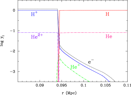
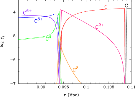
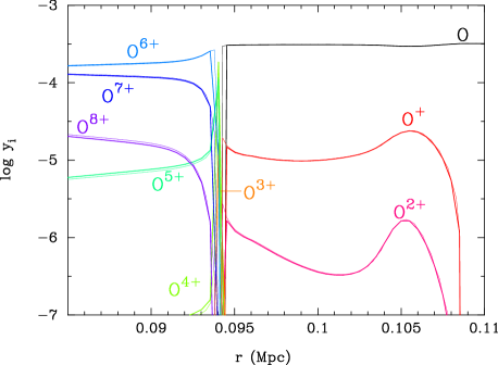
Figure 9: Chemical abundances of hydrogen, helium and electron (top panel), carbon (middle) and oxygen (bottom) as a function of the radius $r$ at $t=0.35$ Myr (3) for the case of $\delta_{\rm b}=10^{3}$. Thick (thin) lines correspond to calculations with grid number 400 (800).

4.1.2 Case of $\delta_{\rm b}=10^{4}$

Figure 10 shows the pressure (upper panel) and the velocity (lower) as a function of the radius at time $t=0.12$ Myr (1), 0.24 Myr (2), 0.35 Myr (3), 0.47 Myr (4) and 0.59 Myr (5). A step in pressure exist at $r\sim 0.04$ Mpc (the ionization front of He ii). Sharp decreases in pressure cause some structures in velocity which are seen in Fig. 10. Dotted lines show the same physical quantities for another calculation with grid number of 800.

Figure 10: Pressure (upper panel) and velocity (lower) as a function of the radius $r$ at time $t$=0.12 Myr (1), 0.24 Myr (2), 0.35 Myr (3), 0.47 Myr (4) and 0.59 Myr (5) for the case of $\delta_{\rm b}=10^{4}$. Solid (dotted) lines correspond to calculations with grid number 400 (800).

Figure 11 shows chemical abundances of hydrogen, helium and electron (top panel), carbon (middle) and oxygen (bottom) as a function of the radius $r$ at $t=0.35$ Myr (3). Thin solid lines show the same physical quantities calculated with 800 grid points.

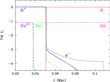
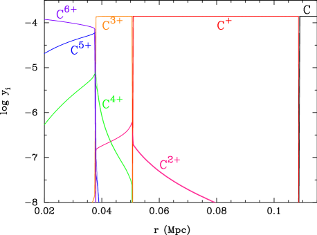
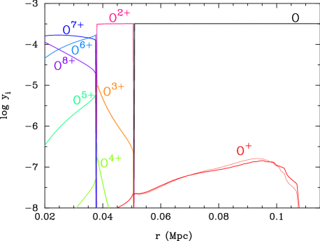
Figure 11: Chemical abundances of hydrogen, helium and electron (top panel), carbon (middle) and oxygen (bottom) as a function of the radius $r$ at $t=0.35$ Myr (3) for the case of $\delta_{\rm b}=10^{4}$. Thick (thin) lines correspond to calculations with grid number 400 (800).

4.1.3 Effect of UV background

A UV background can cause a heating of gas. In addition, even a weak UV background in the epoch of the hydrogen reionization had quickly ionized neutral carbon with low ionization potential. For example, consider a region of density excess $\delta_{\rm b}=10^{4}$ at $1+z=10$ exposed to a soft UV background with flux $J=10^{-21}J_{21}(E_{\gamma}/13.6~{}{\rm eV})^{-1.5}$ ergs s^-1 cm^-2 Hz^-1 str^-1 in $E_{\gamma}\lid 13.6$ eV. Assuming the gas temperature of 300 K and that the abundance of electron is equal to that of C ii, the equilibrium abundance ratio of C ii to C i is approximately $n_{\rm C_{II}}/n_{\rm C_{I}}=3.8\times 10^{4}~{}J_{21}$. Even a $J_{21}$ value as low as $10^{-4}$, which is possibly achieved very soon after the onset of Population III star formation (see e.g. Haiman, Abel & Rees, 2000) is enough to ionize most of the carbon. In order to check effects of UV background the following extra calculations are performed.

We assume that there are UV sources which appear $0.1H(z=8.7)^{-1}$ before the onset of the point source. $H(z)^{-1}$ is the Hubble time at redshift $z$, and the flat $\Lambda$CDM universe has been assumed, i.e., $H(z)=H_{0}\sqrt[]{\mathstrut\Omega_{\rm m}(1+z)^{3}+\Omega_{\Lambda}}$. The UV background is, therefore, switched on at $z=9.8$ corresponding to the cosmic age of $0.50$ Gyr.

The UV spectrum is roughly given by

$$J_{\nu}=\left\{\begin{array}[]{l}10^{-21}J_{21}~{}(E_{\gamma}/13.6~{}{\rm eV})^{-1.5}~{}{\rm ergs/s/Hz/str}\\ ~{}~{}~{}~{}~{}~{}~{}~{}~{}~{}{\rm for}~{}E_{\gamma}\lid 13.6~{}{\rm eV}\\ 10^{-21}J_{21}\epsilon_{X}(E_{\gamma}/13.6~{}{\rm eV})^{-1.5}~{}{\rm ergs/s/Hz/str}\\ \times\exp[-10^{22}(\sigma^{\rm ion}_{{\rm H_{I}},{\rm cm}^{2}}+0.08\sigma^{\rm ion}_{{\rm He_{I}},{\rm cm}^{2}})]\\ ~{}~{}~{}~{}~{}~{}~{}~{}~{}~{}{\rm for}~{}E_{\gamma}>13.6~{}{\rm eV},\end{array}\right.$$ (69)

where $\sigma^{\rm ion}_{i,{\rm cm}^{2}}$ is the photoionization cross section of $i$ in units of cm². This form is adopted from Haiman et al. (2000) although the modulation factor is neglected, and the spectral index is different. The exponential factor corresponds to the absorption above ionization energy threshold of H i by the neutral IGM under the assumption of a hydrogen column density of $N_{\rm H}=10^{22}$ cm^-2. A parameter $\epsilon_{X}$ is the ratio of X-ray to UV flux: $\epsilon_{X}=0$ for pure stellar sources and $\epsilon_{X}\sim 1$ for typical quasar spectra. The parameter $\epsilon_{X}$ would thus parametrize fractions of contributions of stars and quasars. Two cases of $\epsilon_{X}=0$ (soft) and 1 (hard spectrum) with a fixed value of $J_{21}=1$ are calculated assuming the homogeneous UV backgrounds.

In both cases of $\epsilon=0$ and 1, C i is completely ionized after the UV exposures over 0.1 Hubble time at $z=8.7$ (88 Myr). In the case of $\epsilon=1$, the ionization by hard UV photons heat up the homogeneous gas. The temperature at $z=8.7$ is then $10^{3}$ K. We first calculated one-zone chemical abundances in an exposure to the UV background from $z=9.8$ to $8.7$. We then calculated chemical abundances around the point source as a function of radius taking account of ionizations by the point source and the homogeneous UV backgrounds using results of one zone chemical evolution as input.

Figure 12 shows the pressure (upper panel) and the velocity (lower) as a function of the radius at time $t=0.12$ Myr (1), 0.24 Myr (2), 0.35 Myr (3), 0.47 Myr (4) and 0.59 Myr (5). Solid, dashed and dotted lines correspond to cases of a soft, hard and no UV backgrounds which is the same as in Fig. 8, respectively. Calculations for two cases with UV backgrounds are performed with 200 grid points. There is no large difference between values in three cases except for pressure values in the case of hard UV background.

Figure 12: Pressure (upper panel) and velocity (lower) as a function of the radius $r$ at time $t$=0.12 Myr (1), 0.24 Myr (2), 0.35 Myr (3), 0.47 Myr (4) and 0.59 Myr (5) for the case of $\delta_{\rm b}=10^{3}$. Solid, dashed and dotted lines correspond to cases of a soft, hard and no UV backgrounds, respectively.

Figure 13 shows chemical abundances of hydrogen, helium and electron (top panel), carbon (middle) and oxygen (bottom) as a function of the radius $r$ at $t=0.35$ Myr (3). Solid, dashed and dotted lines correspond to cases of a soft, hard and no UV backgrounds which is the same as in Fig. 9, respectively. In the cases with UV backgrounds, C i has already been ionized while in the case of no UV background C i exists outside the light front.

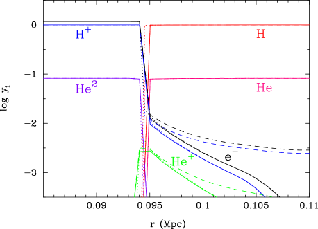
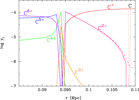
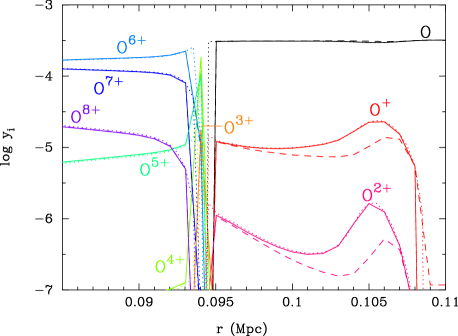
Figure 13: Chemical abundances of hydrogen, helium and electron (top panel), carbon (middle) and oxygen (bottom) as a function of the radius $r$ at $t=0.35$ Myr (3) for the case of $\delta_{\rm b}=10^{3}$. Solid, dashed and dotted lines correspond to cases of a soft, hard and no UV backgrounds, respectively.

4.2 Signals through Fine Structure Transitions

We divide signals by the UV photon pumping into two classes. One is a signal emitted in regions just outside of ionized regions. The other is that of UV photons generated as more energetic than that of the line center frequency and redshifted to the line center when they arrive at radii larger than ionization fronts.

4.2.1 Signals from Ionization Fronts

The UV photons can pump up the energy levels of C i, C ii and O i when they arrive in regions of abundant given chemical species. Since the amount of UV photon is finite, flux densities of the pumping photons are reduced as they pump up. Firstly, we check if there are enough UV photons for mixing the fine structure levels so that the UV pumping can effectively occur inside the light front before arrivals of ionization fronts in the setting of this study.

The ionization time scale at around the ionization front (i.e., an optically thin region) is given by equation (57), and the precise number regarding H i ionization is $\Delta t_{\rm ion}({\rm H_{I}})=2.2\times 10^{8}~{}{\rm s}~{}[r/(0.1~{}{\rm Mpc})]^{2}$. Minimum cross sections for scattering off of UV photons by C i, C ii and O i required for a scattering in the time scale of ionization, i.e., $\Delta t_{\rm ion}({\rm H_{I}})$ is

$$\sigma = \frac{1}{n_{A_{N}}\Delta t_{\rm ion}}$$ (70)

$$= 8.7\times 10^{-15}~{}{\rm cm}^{2}\left(\frac{y_{A_{N}}}{10^{-4}}\right)^{-1}\left(\frac{1+z}{9.7}\right)^{-3}$$

$$\times\left(\frac{\delta_{\rm b}}{10^{3}}\right)^{-1}\left(\frac{r}{0.1~{}{\rm Mpc}}\right)^{-2}.$$

The frequency ranges around the line center of frequency $\nu_{\rm UV}$ which satisfy $\sigma\gid 10^{-14}$ cm² in the case of $T_{\rm gas}=2.3~{}{\rm K}[(1+z)/10]^{2}$ (Loeb & Zaldarriaga, 2004) is $\Delta\nu/\nu_{\rm UV}=6.2\times 10^{-7}$ for the ground state C i atom, $6.8\times 10^{-7}$ for the ground state C ii ion, and $5.2\times 10^{-7}$ for the ground state O i atom. The emission rates $S_{\rm S}$ of UV line photons which interact with C and O before ionizing photons could ionize H i are derived by

$$S_{\rm S}=\frac{L_{\nu_{\rm UV}}}{h\nu_{\rm UV}}\Delta\nu.$$ (71)

Values in the present setting are obtained using equation (43): $S_{\rm S}=3.8\times 10^{52}~{}{\rm s}^{-1}$ for C i, $3.0\times 10^{52}~{}{\rm s}^{-1}$ for C ii, and $2.2\times 10^{52}~{}{\rm s}^{-1}$ for O i.

Figure 14 shows differences between spin temperatures and the CBR temperature in units of K as a function of the radius $r$. In drawing this figure, losses of UV line photons by interaction with atoms and ions are not considered. As will be discussed below, UV line photons are quickly used to pump up the fine structure levels. This figure, then, shows the maximum temperature differences adequate for only regions right beyond the ionizing front where the loss of photons can be neglected.

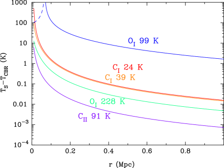
Figure 14: Differences between spin temperatures and the CBR temperature (K) as a function of the radius $r$ (solid lines). The value is negative for the O i 99K line at $r\leq 0.07$ Mpc due to the large population of second excited state of O i by an efficient pumping, and its absolute value is shown (dashed line).

Suppose that ionizing UV photons are mainly used to ionize H i, and that photons of frequency around the UV pumping lines are mainly used to excite and deexcite C i, C ii and O i. We compare the emission rate of ionizing photon per hydrogen number density, i.e., $f_{\rm H_{I}}S_{\gamma}/n_{\rm H}$ with that of line photon per differences of number densities of excited states $i$, i.e., $S_{S}/\Delta n_{A_{N}}^{i}$. Here $\Delta n_{A_{N}}^{i}\equiv n_{A_{N}}^{i}(T_{\rm S})-n_{A_{N}}^{i}(T_{\rm CBR})$ was defined, and number densities of excited state $i$, $n_{A_{N}}^{i}(T)$ are described by the steady state spin temperature ($T_{\rm S}$) and that of CBR ($T_{\rm CBR}$), respectively [see equations (1) and (2)]. At $r=0.1$ Mpc, $S_{\rm S}/\Delta n_{\rm C_{I}}^{1}=9.2f_{\rm H_{I}}S_{\gamma}/n_{\rm H}$ and $S_{\rm S}/\Delta n_{\rm C_{I}}^{2}=1.4f_{\rm H_{I}}S_{\gamma}/n_{\rm H}$ for C i, $S_{\rm S}/\Delta n_{\rm C_{II}}^{1}=77f_{\rm H_{I}}S_{\gamma}/n_{\rm H}$ for C ii, and $S_{\rm S}/\Delta n_{\rm O_{I}}^{1}=311f_{\rm H_{I}}S_{\gamma}/n_{\rm H}$ and $S_{\rm S}/\Delta n_{\rm O_{I}}^{2}=248f_{\rm H_{I}}S_{\gamma}/n_{\rm H}$ for O i. It is seen that UV photons which can scatter C and O exist in abundances larger than ionizing photons when normalized to target number densities. The scattering regions, therefore, extend outward faster than ionized regions.

Inside ionization fronts of C i, C ii and O i, UV line photons propagate outward without scattering. When they enter in region with abundant C i, C ii and O i, however, they scatter the species and change the fine structure population. The UV line photons effectively pump low energy level states up to high energy levels until steady states realize. Excited states eventually decay into low states by magnetic dipole photon emission. Repeating pumpings and decays lead to net reduction of number flux of energetic UV line photon which can pump up C and O from low energy states.

The radius scale for this scattering loss is given by those of regions where the steady state spin temperatures can be hold by the flux from the point source. Balances between pumping up and spontaneous decay of excited states in a volume $V=4\pi r_{\rm B}^{2}\Delta r$, with $r_{\rm B}$ the boundary of the C and O ionization and $\Delta r$ the width, are roughly described by

$$4\pi r_{\rm B}^{2}\left(\frac{F_{\nu_{\rm UV}}}{h\nu_{\rm UV}}\Delta\nu_{\rm D}-\Delta r\Delta n_{A_{N}}^{i}A_{ij}\right)\sim 0,$$ (72)

where the UV flux in the frequency range of Doppler width $\Delta\nu_{\rm D}$ is considered in the source term which enter into this region from the boundary $r_{\rm B}$. The radius scale is thus

$$\Delta r\sim\frac{F_{\nu_{\rm UV}}}{h\nu_{\rm UV}}\frac{\Delta\nu_{\rm D}}{\Delta n_{A_{N}}^{i}A_{ij}}.$$ (73)

For the radius of $r=0.1$ Mpc, this equation yields

$$\Delta r= 0.8~{}(\delta_{\rm b}/10^{3})^{-1}T_{\rm gas,K}^{1/2}~{}{\rm pc} {\rm(for~{}the~{}C_{I}~{}24~{}K~{}line)},$$

$$0.02~{}(\delta_{\rm b}/10^{3})^{-1}T_{\rm gas,K}^{1/2}~{}{\rm pc} {\rm(C_{I}~{}39~{}K)},$$

$$0.02~{}(\delta_{\rm b}/10^{3})^{-1}T_{\rm gas,K}^{1/2}~{}{\rm pc} {\rm(C_{II}~{}91~{}K)},$$

$$4\times 10^{-3}~{}(\delta_{\rm b}/10^{3})^{-1}T_{\rm gas,K}^{1/2}~{}{\rm pc} {\rm(O_{I}~{}228~{}K)},$$

$$2~{}(\delta_{\rm b}/10^{3})^{-1}T_{\rm gas,K}^{1/2}~{}{\rm pc} {\rm(O_{I}~{}99~{}K)}.$$

The UV line photons around the line center quickly scatter C and O and decreases during propagations through narrow regions if the density is high as in this calculation.

4.2.2 Signals from Outside of Ionization Fronts

1. Steady state abundances of excited states

   Secondly, signals from excitations by redshifted UV photons are estimated. For simplicity, we assume that UV photons redshifted beyond certain critical frequencies from the blue side instantaneously scatter C and O, and are used for pumping up of the species. The number flux of the UV line photon, i.e., $F_{\nu_{\rm UV}}/(h\nu_{\rm UV})$, should satisfy

   $$\frac{d}{dr}\left(\frac{F_{\nu_{\rm UV}}}{h\nu_{\rm UV}}\right)=-\Delta n_{A_{N}}^{i}A_{ij}+N_{\rm eff}\frac{F_{\nu_{\rm UV}}}{h\nu_{\rm UV}}\frac{\nu_{\rm UV}H(t)}{c},$$ (74)

   where $\Delta n_{A_{N}}^{i}$ is the abundance of excited state $i$, $N_{\rm eff}$ is the effective number of lines which contribute to pumping up C i, C ii and O i of fine structure levels, and defined below. The first term in the right hand side is for spontaneous emission of excited state $i$, while the second is for production by redshifted UV photons. The production term is proportional to the number flux of the UV line photons and the rate of redshift per unit distance, i.e., $|d\nu/dr|\approx|d\nu/(cdt)|=\nu_{\rm UV}H(t)/c$. The steady state for abundances of fine structure levels would be realized in a region between an ionization boundary and the light front. They are described by a balance in equation (74), i.e., $d[F_{\nu_{\rm UV}}/(h\nu_{\rm UV})]/dr=0$, as

   $$\Delta n_{A_{N}}^{i}=N_{\rm eff}\frac{F_{\nu_{\rm UV}}}{h\nu_{\rm UV}}\frac{\nu_{\rm UV}H(t)}{cA_{ij}},$$ (75)

2. Effective number of available UV lines

   UV photons described by a color temperature $T_{\rm UV}$ repeat scattering C and O species through the UV photon pumping, and eventually relax to the color temperature of the fine structure spin states which is approximately given by the CBR temperature if the UV photon pumping occurs frequently enough. In this process, chemical species in excited states which have been pumped up by UV line photons can emit line photons corresponding to the fine structure transitions. The effective number $N_{\rm eff}$ is given as follows taking account of the relaxation.

   1. C ii

      For the C ii, the net increase in the number of ions in the excited state is given by the net increase in the number of photons corresponding to the transition ²P${}_{3/2}\rightarrow^{2}$D_3/2 (see Table 1) after the relaxation process through the UV scattering. $N_{\rm eff}$ is, therefore, given by

      $$N_{\rm eff}=\frac{2}{1+\exp{(-T_{\ast}/T_{\rm CBR})}}-1,$$ (76)

      where the first term in right hand side is the relative number of line in the final relaxed state, and the second term is that in the initial state, that is equal to unity. In the final state, initial UV photon flux for two lines, i.e., ²P${}_{3/2}\rightarrow^{2}$D_3/2 and ²P${}_{1/2}\rightarrow^{2}$D_3/2 is distributed to the two lines by the equilibrium fraction of

      $$\frac{F_{{}^{2}{\rm P}_{3/2}}}{F_{{}^{2}{\rm P}_{1/2}}}=\exp{(T_{\ast}/T_{\rm CBR})},$$ (77)

      which realizes the balance between pumping rates of both directions, i.e.,

      $$n_{0}F_{0}\sigma_{0\rightarrow u\rightarrow 1}=n_{1}F_{1}\sigma_{1\rightarrow u\rightarrow 0},$$ (78)

      where $F_{0}=F_{{}^{2}{\rm P}_{1/2}}$, $F_{1}=F_{{}^{2}{\rm P}_{3/2}}$, and $\sigma_{i\rightarrow u\rightarrow j}=\sigma(i\rightarrow~{}u)\times A_{uj}/(\sum_{k}A_{uk})$ is the cross section of process $i\rightarrow u\rightarrow j$ [cf. equation (22)].

   2. O i

      Similarly, effective numbers for the first and second excited states of O i are given by

      $$N_{\rm eff,1}=\frac{3}{1+\exp{(-T_{\ast 2}/T_{\rm CBR})}\left[1+\exp{(-T_{\ast}/T_{\rm CBR})}\right]}-1,$$ (79)

      $$N_{\rm eff,2}=\frac{3\exp{(-T_{\ast 2}/T_{\rm CBR})}}{1+\exp{(-T_{\ast 2}/T_{\rm CBR})}\left[1+\exp{(-T_{\ast}/T_{\rm CBR})}\right]}-1,$$ (80)

      respectively. Here it was assumed that the UV photon pumping of the first excited state of O i is efficient as well as that of the ground state as a sufficient condition for the equilibrium UV line photon. Since the abundance of the excited O i (³P₁) state is rather small [$g_{0}n_{1}/(g_{1}n_{0})\sim\exp(-228~{}{\rm K}/T_{\rm CBR})=2.3\times 10^{-4}$ for $1+z=10$], this assumption is satisfied in environments of high O i densities. If the density excess is $\delta_{\rm b}\sim 10^{4}$, the equilibrium UV flux can realize [equation (86)], and a contamination from a collisional signal is still small if the gas temperature is not so high (Section 2.1.2). If the density excess is smaller, the number of UV lines through which UV photons effectively scatter becomes smaller. If the density of O i is as small as $\delta_{\rm b}\sim 1$, only the UV pumping of the ground state is efficient. Signals of the O i fine structure lines then originate from pumping of the ground state by a part of UV line photons. In such a case of small O i number density (Hernández-Monteagudo et al., 2007), signals of both O i 228 K and 91 K would become emissions and their intensities smaller than the estimations given here.

   3. C i

      As for C i, two contributions through the upper levels ³P₁ and ³P₂ exist. The effective numbers for the first and second excited states are then given by

      $$N_{\rm eff,1} = \frac{3}{1+\exp{(-T_{\ast 2}/T_{\rm CBR})}\left[1+\exp{(-T_{\ast}/T_{\rm CBR})}\right]}-1$$ (81)

      $$+\frac{2}{1+\exp{(-T_{\ast 2}/T_{\rm CBR})}}-1,$$

      $$N_{\rm eff,2} = \frac{3\exp{(-T_{\ast 2}/T_{\rm CBR})}}{1+\exp{(-T_{\ast 2}/T_{\rm CBR})}\left[1+\exp{(-T_{\ast}/T_{\rm CBR})}\right]}-1$$ (82)

      $$+\frac{2\exp{(-T_{\ast 2}/T_{\rm CBR})}}{1+\exp{(-T_{\ast 2}/T_{\rm CBR})}}-1,$$

      respectively. The first and second lines in right hand sides of the above two equations correspond to the contributions of UV pumping through the ³P₁ and ³P₂ levels, respectively. Since the number density of excited state C i (³P₁) is large [$g_{0}n_{1}/(g_{1}n_{0})\sim\exp(-24~{}{\rm K}/T_{\rm CBR})=0.41$ for $1+z=10$], the equilibrium abundances realize relatively easily.

3. Scattering rate

   A steady state scattering rate [cf. equation (21) for the rate derived neglecting the scattering loss] in the region outside of ionization front is estimated as follows: The balance between a rate of scattering and that of depletion of UV line photons whose frequencies are redshifted over critical frequencies is described as

   $$n_{A_{N}}^{i}P_{\nu}=N_{\rm eff}\frac{F_{\nu_{\rm UV}}}{h\nu_{\rm UV}}\frac{\nu_{\rm UV}H(t)}{c}.$$ (83)

   We obtain the steady state $P_{\nu}$ value from this equation, i.e.,

   $$P_{\nu} = \frac{1}{n_{A_{N}}^{i}}N_{\rm eff}\frac{L_{\nu}/(h\nu)}{4\pi r^{2}}\frac{\nu_{\rm UV}H(t)}{c}$$ (84)

   $$= 3.3\times 10^{-10}~{}{\rm s}^{-1}\left(\frac{\lambda_{lu}}{\lambda_{\alpha}}\right)^{\alpha_{\rm S}}N_{\rm eff}\left(\frac{1+z}{10}\right)^{-3}$$

   $$\times\left(\frac{\delta_{\rm b}Y_{A_{N}}^{i}}{10^{-4}}\right)^{-1}\frac{\left(\nu L_{\nu}\right)_{\alpha,47}}{(r_{\rm Mpc}/0.1)^{2}}\left(\frac{H(z)}{3.7\times 10^{-17}~{}{\rm s}^{-1}}\right).$$

   See Section 2.1.2 for effects of UV photons on spin temperatures.

4. Signals through the lowest-energy UV lines

   Figure 15 shows the differential antenna temperatures, i.e., the brightness temperature $T_{\rm b}$ minus CBR temperature in units of mK as a function of the radius. For this figure we assume that the abundances of C i, C ii and O i are their maximum values, i.e., $y_{\rm C_{I}}=1.4\times 10^{-4}$, $y_{\rm C_{II}}=1.4\times 10^{-4}$, and $y_{\rm O_{I}}=3.2\times 10^{-4}$, respectively. The differential antenna temperatures are derived with the following equation which is satisfied when $T_{\rm b}-T_{\rm CBR}\ll T_{\rm CBR}$:

   $$\Delta\equiv\frac{T_{\rm b}-T_{\rm CBR}}{T_{\rm CBR}}=\frac{\Delta I_{\nu}}{B_{\nu}(T_{\rm CBR})}\frac{\exp(T_{\ast}/T_{\rm CBR})-1}{(T_{\ast}/T_{\rm CBR})\exp(T_{\ast}/T_{\rm CBR})}.$$ (85)

   Since the differential antenna temperature is rather small, signals of these magnitudes would not be detected with existing radio telescope or the planned Atacama Large Millimeter/submillimeter Array (ALMA).

   

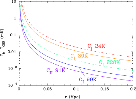
   Figure 15: Differential antenna temperatures (mK) as a function of the radius. Solid curves are for positive values, while dashed curves are for absolute values of negative ones. The respective curves are derived under the assumption that the elements (C and O) are completely in the chemical species (C i, C ii and O i), and therefore indicate maximum values for respective lines.

5. Signals through all available UV lines

   So far only the effects of lines shown in Fig. 1 are analyzed. There are, however, many other lines of energies less than the ionization threshold of H i which can mix fine structure levels. We then include effects of those lines. Lines available for pumping up the C and O species in the fine structure levels should satisfy a requirement: the time scale of UV pumping of C or O by photons of line center frequencies $\Delta t_{\rm pump}$ is shorter than that of redshift $\Delta t_{\rm red}$. If this is not satisfied, only a part ($\sim\Delta t_{\rm red}/\Delta t_{\rm pump}$) of the UV line photons can scatter C or O before their frequencies are removed from the line center and they become inert. Using $\Delta t_{\rm pump}=\sqrt[]{\mathstrut\pi}\Delta\nu_{\rm D}/(n_{A_{N}}\sigma)$ (Rybicki & Lightman, 1979) and $\Delta t_{\rm red}=\Delta\nu_{\rm D}/[\nu_{\rm UV}H(t)]$, and defining $\bar{A}$ by $\sigma\sim\lambda^{2}/(8\pi)\bar{A}$ [cf. equation (22)], a relation is obtained, i.e,

   $$\frac{\Delta t_{\rm pump}}{\Delta t_{\rm red}} = \nu_{{\rm UV},15}^{3}\left(\frac{1+z}{10}\right)^{-3/2}\left(\frac{\delta_{\rm b}Y_{A_{N}}}{10^{-4}}\right)^{-1}$$ (86)

   $$\times\left(\frac{3.2\times 10^{6}~{}{\rm s}^{-1}}{\bar{A}}\right),$$

   where $\nu_{{\rm UV},15}$ is the line center frequency in units of $10^{15}$ s^-1. The lines contributing to the pumping up of fine structure levels should have Einstein $A$-coefficient enough large in order to satisfy $\Delta t_{\rm pump}/\Delta t_{\rm red}<1$. This condition tends to be met in environments of high $\delta_{\rm b}Y_{A_{N}}$ values. If the two timescales are nearly identical, i.e., $\Delta t_{\rm pump}\sim\Delta t_{\rm red}$, the depletion at the UV pumping of UV line photons balances with the production via cosmological redshift. In such a situation, the steady state UV line flux and the resulting line scattering rate [equation (84)] are relatively large.

   Assuming that all UV lines of $A>10^{6}$ s^-1 contribute to the pumping up, for example, signals through the C and O species are calculated using atomic data from Ralchenko et al. (2008). Figure 16 shows differential antenna temperatures when contributions from all UV lines of $A>10^{6}$ s^-1 are included. The signals for C i and O i are enhanced relative to curves in Fig. 15 since many additional strong lines exist. On the other hand, the signal for C ii is not enhanced much since only two upper states, one of which is the ²D_3/2 shown in Fig. 1, are available.

   

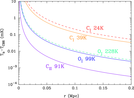
   Figure 16: Same as in Fig 15 but including the effects of all UV lines of spontaneous emission rates larger than 10⁶ s^-1.

4.3 Flux Densities of the Point Source

Total flux densities, i.e., $S=\int S_{\nu}~{}d\nu$, from IGM via the fine structure line emission or absorption are estimated with the calculated results of the time evolution of the chemical structure. We suppose that a point source starts lighting at time $t=0$ at redshift $z=8.7$. The comoving distance to the source, $r_{\rm S}$, is defined by

$$r_{\rm S}=\int_{t_{\rm S}}^{t_{0}}\frac{cdt}{a(t)}=\frac{c}{H_{0}}\int_{a_{\rm S}}^{1}\frac{da}{\sqrt[]{\mathstrut\Omega_{\rm m}a+(1-\Omega_{\rm m})a^{4}}},$$ (87)

where $a_{\rm S}$ and $t_{\rm S}$ are the scale factor and the corresponding time of the universe when the source exists, and $t_{0}$ is the age of the present universe.

We introduce two dimensional Cartesian coordinates. The source and the observer are assumed to locate at the origin and $x=\infty$. The flux density in the redshifted fine structure frequency which is measured on the earth is given by

$$S_{\rm fs}^{i}\approx\frac{1}{(1+z)^{4}}\frac{h\nu_{0}A_{ij}}{r_{\rm S}^{2}}\int_{0}^{r_{\rm D}}ydy\int_{-x_{\rm max}}^{x_{\rm max}}dx~{}\Delta n_{A_{N}}^{i}(r,t+x/c),$$ (88)

where $r_{\rm D}\sim 0.2$ Mpc is the radius of the calculation domain, $x_{\rm max}=\sqrt[]{\mathstrut r_{\rm D}^{2}-y^{2}}$, and $r=\sqrt[]{\mathstrut x^{2}+y^{2}}$ is the radius from the source. We assume that the UV lines with emission rates of $A\gid 10^{6}$ s^-1 contribute to the UV pumping of C or O when the abundance is enough large, i.e., $Y_{A_{N}}\gid 10^{-4}$. The value of $\Delta n_{A_{N}}^{i}(r,t+x/c)$ is thus given by equation (75) if $Y_{A_{N}}(r,t+x/c)$ is larger than $10^{-4}$. The value is set to be zero otherwise. Note that the effect of the time delay is included in $\Delta n_{A_{N}}^{i}(r,t+x/c)$ since ionization fronts propagate at sub-light speeds.

Figure 17 shows the total flux densities emitted through the C ii and O i fine structure lines in the calculated domain of $r\lid 0.2$ Mpc in units of nJy GHz. The calculated result for the case of $\delta_{\rm b}=10^{3}$ is used for this estimation. As the light propagates outwards, the volume of the region experiencing the UV pumping of C and O increases. The emissions (solid lines) and the absorption (dashed line) triggered by redshifted UV photons are then enhanced. For this figure we assume that the chemical abundances as a function of the radius are fixed after the time of the end of calculation, i.e., $t_{\rm end}$ at values of $t_{\rm end}$. This is because we do not have results of $t>t_{\rm end}$ which are necessary to calculate the total flux densities due to the time delay effect in equation (88). No C i region exists inside the light radius in our calculation. There are large amounts of ionizing photons of C i escaping from shielding since the threshold energy of C i (11.3 eV) is lower than that of H i (13.6 eV). Thick lines correspond to the standard case of no UV background, while thin lines correspond to two cases of a soft and hard UV backgrounds (Section 4.1.3).

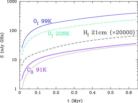
Figure 17: Total flux densities (nJy GHz) emitted through the C_II and O_I fine structure lines and the H i 21 cm line in the calculated region for the case of $\delta_{\rm b}=10^{3}$. The values which we would measure at $z=0$ are shown as a function of the time from the start of the hydrodynamical calculation. Solid lines correspond to emissions, while a dashed line is for absorption. Thick lines correspond to the standard case of no UV background, while thin lines correspond to two cases of a soft and hard UV backgrounds.

In Fig. 17, the total flux density for the H i 21 cm line is also shown. The flux density is given by

$$S_{21}\approx\frac{1}{(1+z)^{4}}\frac{h\nu_{21}A_{21}}{r_{\rm S}^{2}}\int_{0}^{r_{\rm D}}ydy\int_{-x_{\rm max}}^{x_{\rm max}}dx~{}\Delta n_{\rm H}^{1}(r,t+x/c),$$ (89)

where $\nu_{21}=1.4$ GHz is the frequency corresponding to the 21 cm line transition, $A_{21}=2.9\times 10^{-15}$ s^-1 is the spontaneous emission rate of the hyperfine structure transition, and $\Delta n_{\rm H}^{1}$ is the difference of the number abundance of the excited level of H i hyperfine structure (n${}_{\rm H}^{1}$) in the presence of the UV radiation field from that without the UV field.

H i regions which are irradiated with UV photons are heated predominantly via photoionization. The heating rate is given by equation (39). The gas temperature in the H i region with enough UV flux would, therefore, be higher while that in region with strongly shielded UV flux would be lower than the CBR temperature. Note that the Ly$\alpha$ scattering provides a negligible heating (e.g., Chen & Miralda-Escude, 2004).

The spin temperature of the H i hyperfine structure, i.e., $T_{\rm S}$, is usually much larger than the transition temperature $T_{\ast}\equiv h\nu_{21}/k=0.068$ K. The abundance of the excited state is then given by

$$n_{\rm H}^{1}=\frac{3\exp(-T_{\ast}/T_{\rm S})}{1+3\exp(-T_{\ast}/T_{\rm S})}n_{\rm H_{I}}\approx\frac{3}{4}\left(1-\frac{1}{4}\frac{T_{\ast}}{T_{\rm S}}\right)n_{\rm H_{I}}.$$

We define $T_{\rm S}$ and $T_{\rm BG}$ as the spin temperature in the UV radiation fields and that without it. Although the effect of the collisional excitation of the hyperfine structure line is not negligible in regions of high densities, we here neglect the effect in order to derive the maximum effect of the Ly$\alpha$ pumping on the 21 cm emission. Under this assumption, when there is no UV radiation field, the spin temperature is purely described by the CBR temperature, i.e., $T_{\rm BG}=T_{\rm CBR}$. Since the spin temperature in the H i region at radius $r\la O(0.1~{}{\rm Mpc})$ is very close to the H i gas temperature (Madau et al., 1997), a situation of $T_{\rm S}>T_{\rm BG}$ is realized if the UV radiation field is not severely shielded. From this equation, we obtain

$$\Delta n_{\rm H}^{1}\approx\frac{3}{16}\frac{T_{\ast}}{T_{\rm CBR}}n_{\rm H_{I}}$$ (90)

On the other hand, if the UV radiation field is shielded, an environment of $T_{\rm S}<T_{\rm BG}$ leads to

$$\Delta n_{\rm H}^{1}\approx-\frac{3}{16}\frac{T_{\ast}}{T_{\rm S}}n_{\rm H_{I}}$$ (91)

The line in Fig. 17 was drawn assuming equations (89) and using the calculated results of the H i abundance and the gas temperature as a function of the time and the radius. There is an important difference between the standard, soft UV and hard UV cases. In the hard UV case the gas temperature has been heated up by the UV background. The spin temperature of 21 cm line is then larger than the CBR temperature, i.e., $T_{\rm CBR}=2.725(1+z)$ K. The 21 cm signal is, therefore, an emission, and its amplitude is a factor $\sim T_{\rm CBR}/T_{\rm S}$ smaller than that of absorption in cases of $T_{\rm CBR}>T_{\rm S}$ (Scott & Rees, 1990; Madau et al., 1997).

Figure 18 shows the total flux densities emitted through the C ii and O i fine structure lines and the H i 21 cm line in the calculated domain of $r\lid 0.2$ Mpc for the case of $\delta_{\rm b}=10^{4}$. The high density of the matter causes a slow expansion of ionized regions. There are larger volume of C ii and O i regions which are affected by the UV pumping than in the case of $\delta_{\rm b}=10^{3}$. The flux densities are thus enhanced in this high density case.

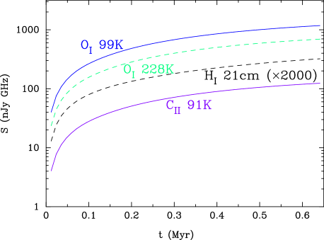
Figure 18: Same as in Fig 17 for the case of $\delta_{\rm b}=10^{4}$.

4.4 Effect of Collisional Excitation

In dense regions, an effect of collisional excitation on spin temperatures of fine structure transitions can not be neglected. For example, our calculations are performed under the assumption that the number density of hydrogen is $n_{\rm H}\sim 2\times 10^{-1}(\delta_{\rm b}/10^{3})[(1+z)/10]^{3}$ cm^-3. Collisional excitations and deexcitations of C i and C ii proceed by interactions of those species mainly with surrounding H i and electron. O i atoms can interact with surrounding H i and electron to get excited or deexcited (see Figs. 9 and 11). The deexcitation rates taken from (Hollenbach & McKee, 1989) are listed in Table 1. Collisions contribute to spin temperatures with their efficiency proportional to collisional (de)excitation rates, i.e.,

$$C_{ij} \sim 2\times 10^{-11}~{}{\rm s}^{-1}\left(\frac{\delta_{\rm b}}{10^{3}}\right)\left(\frac{1+z}{10}\right)^{3}y_{\rm target}$$ (92)

$$\times\left(\frac{\gamma_{ij}}{10^{-10}~{}{\rm cm}^{-3}~{}{\rm s}^{-1}}\right).$$

These rates are less than spontaneous emission rates of the fine structure transitions, and possibly of similar magnitudes to UV pumping rates [equations (21) and (84)]. If the gas density of the observed region were high, kinetic temperatures of C i, C ii and O i can be imprinted on the spin temperatures through the collisional excitation (Section 2.1.2).

Signals originating from collisions need to be small in order to detect signals from the pure UV pumping related to ionizing sources of the universe. The best site to look for is a region which meets both of the following two conditions.

1. a large region of moderate density. It does not emit signals of collisional (de)excitations. The signals from this region separate in frequency from those from surrounding dense regions where spin temperatures include large contribution of collisions.

2. a region where ionizing UV photons are effectively shielded and non-ionizing UV photons are not shielded and exist abundantly. C i, C ii and O i can exist without being ionized, and a UV pumping by redshifted UV photons is operative there.

4.5 Observational Constraint on Physical Properties

When one detect a line signal from a region whose physical condition is not known in advance from any different observation, it is not clear whether the signal originated from a UV dominated region or a collision dominated region. Signals of different lines are, therefore, necessary to estimate the physical condition. A line signal is determined by a physical condition of observed region specified by the density, kinetic temperature and environmental UV flux (absolute value and spectrum). Conversely, a signal of a certain metal line could provide a constraint on physical parameters to satisfy a condition which possibly realizes the detected signal. If signals of more than one different lines are detected from the same region, respective constraints on the parameters are obtained since a ratio between excitation rates by UV photons and collision are different for respective transitions corresponding to different lines. Ideally parameters can then be determined and one can estimate whether the signal is from UV photons or from collisions (for individual lines).

We describe an example of how to constrain physical parameters of observed regions for demonstration assuming that line signals of C ii 91 K, O i 228K and 99K were detected. We note that a more precise estimation of line signals is highly desirable. Since the precise propagation of UV photons which excite C i, C ii and O i is not addressed in this study, it should be studied. For the moment, we assume that all UV line photons experience effective scattering of C ii and O i although this assumption would not hold for low density region (see Section 4.2.2).

We suppose that three line signals at $z=8.7$ are detected: $T_{\rm b}-T_{\rm CBR}=(1.2\pm 0.4)\times 10^{-3}$ mK for C ii 91 K, $-(1.2\pm 0.4)\times 10^{-2}$ mK for O i 228K and $(9.8\pm 3.3)\times 10^{-3}$ mK for O i 99K. Parameters to be constrained are, for example, $n_{\rm H_{I}}$, $y_{\rm C_{II}}$, $y_{\rm O_{I}}$, the UV flux at the Ly$\alpha$ frequency, i.e., $F_{\alpha}$, and the spectral index, i.e., $\alpha_{\rm S}$. The dependence of signals on spectral index (or UV color temperature $T_{\rm UV}$) is relatively small (see Fig. 2–5). We then neglect it and fix the value to be $\alpha_{\rm S}=3/2$. The carbon and oxygen abundances, i.e., $y_{\rm C_{II}}$ and $y_{\rm O_{I}}$, should be estimated anyhow since the values and the ratio between them in high redshifts are not know precisely. Detailed theoretical studies on the cosmic chemical evolution may help this estimation (e.g., Kobayashi et al., 2007). We assume that the abundances, $y_{\rm C_{II}}$ and $y_{\rm O_{I}}$, are the same as those of present ISM. The physical parameters in the present setting is then $n_{\rm H_{I}}$, $T_{\rm gas}$ and $F_{\alpha}$. Effects of the UV pumping (Section 4.2.2) and the collision (Section 2.1.2) are calculated.

Figure 19 shows a parameter region in the 3D space of $n_{\rm H}$, $T_{\rm gas}$ and $F_{\alpha}$ in which magnitudes of observed signals are reproduced. The marks of $+$, $\ast$ and $\times$ correspond to parameter sets which fail to predict observed line signals except for only one line signal of C ii 91 K, O i 228 K and O i 99 K, respectively. The squares and triangles correspond to parameter sets which predicts two right signals (C ii 91 K and O i 99 K) and (O i 228 K and 99K), respectively. The circles correspond to parameter sets which rightly predicts all three line signals.

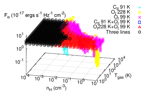
Figure 19: An example of estimation of physical parameters, i.e., the H i number density ($n_{\rm H}$), the gas temperature ($T_{\rm gas}$) and the UV flux at Ly$\alpha$ frequency ($F_{\alpha}$). The marks of $+$, $\ast$ and $\times$ correspond to parameter sets which predict line signals consistent with only one observed line signal of C ii 91 K, O i 228 K and O i 99 K, respectively. The squares and triangles correspond to parameter sets which predicts two right signals (C ii 91 K and O i 99 K) and (O i 228 K and 99K), respectively. The circles correspond to parameter sets which rightly predicts all three line signals. See text for the assumed observational signals and an explanation of adopted model.

4.6 Redshift Dependence of Signals

Signals are different in magnitude between sources of different redshifts. As seen in equation (75), the line emission is proportional to the UV flux $F_{\nu_{\rm UV}}\propto r^{-2}$ [cf. equation (49)] and the Hubble expansion rate $H(z)$. When one fixes the angle $\theta$ between a source and a position $r$ away from it in the direction perpendicular to the line of sight, there is a relation between the redshift and the position, i.e.,

$$\theta=\frac{r(1+z)}{r_{\rm S}}.$$ (93)

Figure 20 shows the differential antenna temperatures in units of mK at the fixed angle of $\theta=5\arcsec$ from the point source of the present setting as a function of the redshift under the assumption that the observed region is abundant in C i, C ii and O i in drawing respective lines.

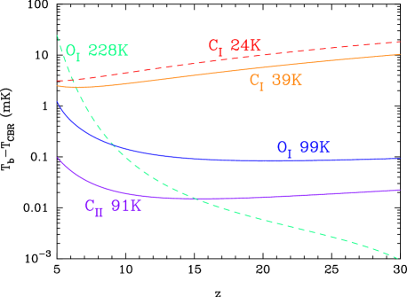
Figure 20: Differential antenna temperatures (mK) at the fixed angle $\theta=5\arcsec$ in the sky from the direction to the point source as a function of the redshift.

The shape of curves in this figure is understood as follows. If a difference between the spin temperature and the CBR temperature is very small, i.e., $\Delta T_{\rm S}\equiv T_{\rm S}-T_{\rm CBR}\ll T_{\rm CBR}$, then it is approximately given by

$$T_{\rm b}-T_{\rm CBR}=\Delta T_{\rm S}\tau.$$ (94)

In the case of two level states, for example, if the population fraction of the ground state is dominant and the contribution of the UV pumping to the excitation is small, then the spin temperature is given by

$$\Delta T_{\rm S}\sim\frac{\Delta n_{1}}{n_{0}}\frac{g_{0}}{g_{1}}\frac{T_{\rm CBR}^{2}}{T_{\ast}}\exp\left(\frac{T_{\ast}}{T_{\rm CBR}}\right).$$ (95)

The differential abundance of the excited state is proportional to the Hubble expansion rate, i.e., $\Delta n_{1}\propto H(t)\propto(1+z)^{3/2}$ [equation (75)]. The abundance of the ground state scales as $n_{0}\propto(1+z)^{3}$, while the optical depth scales as $\tau\propto(1+z)^{3/2}$ [equation (19)]. Ultimately there is a rough scaling of

$$T_{\rm b}-T_{\rm CBR}\propto(1+z)^{2}\exp\{T_{\ast}/[2.725(1+z)~{}{\rm K}]\}.$$ (96)

At low redshift the CBR temperature is low, and the differential temperature increases with the decreasing redshift. At high redshift the differential temperature increases with the increasing redshift mainly through the $(1+z)^{2}$ factor in equation (96) and the fact that the physical scale corresponding to a fixed angular scale of object at higher redshift is smaller in the $\Lambda$CDM model adopted in the present study.

4.7 Detectability

Signals through the C i lines are largest as seen in Fig. 16. If the signals of UV photons are not contaminated by other signals at around the same redshift, we would detect them. The signal predicted in this calculation is $\sim 1$ mK at 0.05 Mpc (11$\arcsec$ in the case of $z=8.7$) if a neutral C i region exists at the distance. This is much larger than the background noise measured with WMAP in a frequency range of $\nu\ga 100$ GHz of $T_{\rm bg}\la 0.02$ mK mainly from vibrational dust emission (Gold et al., 2010). Figure 21 shows a simulation of a signal of UV photons emitted in the early universe at $z=8.7$ through the C i 38K line. The contour map of the differential antenna temperatures in units of mK is drawn on the plane of the angle (arcsec) and the velocity shifts (km s^-1). For this figure it is assumed that a neutral C i region affected by the UV pumping exists in the region of 0.03 Mpc $\lid r\lid$ 0.06 Mpc from the point source.

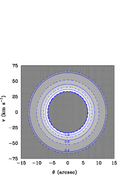
Figure 21: Contour map of the differential antenna temperature (mK) of the C i 38 K line as a function of the angle (arcsec) and the velocity shift (km s^-1) when a neutral C i region affected by the UV pumping exists in the region of 0.03 Mpc $\leq r\leq$ 0.06 Mpc.

Concerning the detectability, a signal of $\sim 1$ mK will be seen with the ALMA. For example, a 1 mK signal emitted through the C i 38 K line at redshift $z=6.3$ will be seen by the 12m Array using the Receiver Band of No. 3 for observations of extended sources at one sigma level if the following parameters are selected: effective bandwidth of 5.3 MHz corresponding to the scale of $\sim 0.02$ Mpc, beamsize of 3$\arcsec$75, and exposure time of 7.6 hr. The ALMA Sensitivity Calculator was used for this estimation. Signals from C ii and O i regions will be detected by future observations to come after the ALMA.

5 Conclusions

The reionization history of the universe at early epoch of redshift $z\sim 10$ is not know precisely yet. We study signals of the cosmological reionization which would have been left on the cosmic background radiation (CBR) through a series of excitations of fine structure levels of C i, C ii and O i and following emissions (absorption) of line photons. Since the reionization of the universe would have proceeded inhomogeneously in space, regions of neutral or low ionization states irradiated by non-ionizing ultraviolet (UV) photons naturally exist during the reionization epoch. Non-ionizing UV photons interact with C and O to excite them to unstable excited states. This excitation followed by decays of the excited states leads to an excitation of fine structure levels. Since the UV photons as a source of the reionization produce signals through fine structure lines in C i, C ii or O i regions, some information on the reionization may be obtained by observations for these lines.

Essentially, one ionizing photon can produce one line photon for a fine structure transition by scattering with C and O species. Strong signals are, therefore, emitted at locations near strong sources of UV emission with large flux of UV photon. We then assume a strong point source such as quasi-stellar object (QSO) which starts lighting in the early universe, and calculate the evolution of ionized region utilizing a non-equilibrium chemical reaction network. A rough picture of ionization is shown by this calculation that C i, C ii and O i regions irradiated by nonionizing UV line photons can exist at locations where ionizing UV photons are effectively shielded by dense H i regions.

There are two classes of UV photons available for the UV pumping of fine structure levels:

1. photons of frequencies just around the fine structure lines at the boundary between ionized region and non-ionized region for C i, C ii and O i,

2. photons which are emitted as more energetic photons at point source and redshifted toward the transition energies of fine structures in C i, C ii and O i regions.

At ionization boundaries, UV photons which can excite the fine structure levels are immediately lost since they are used by the UV pumping. It is then predicted that very small regions emitting line photons energized by UV sources would exist at ionization boundaries. However, the signals of the latter class of UV photons is expected to be stronger than those of the first.

Outside the ionization boundaries, redshifted UV photons can leave their signatures possibly over wide region. The ratios between UV intensities of respective fine structure lines are changed in the relaxation process through scattering with the C and O species, and are affected by the spin states of C and O. Neutral H i regions near strong UV sources emit signals of UV photons available until the relaxation is completed.

Those signals of UV photons could be contaminated by signals of collisional excitations if densities in observed regions were large. Regions of intermediate densities might be good sites to investigate for signals of the reionization since an effective UV pumping is possible in denser region where an effect of collisional excitation is also larger.

The dependence of magnitudes of signals on the source redshift is shown, and the detectability of such signals is discussed taking the Atacama Large Millimeter/submillimeter Array (ALMA) as an example. Although the magnitudes of signals depend on physical environments of observed points, which are roughly described by many fixed parameters in this study, detections of fine structure line of C i, C ii and O i might be possible with the ALMA or future projects.

Appendix A Number fractions of photon ionizing H I, He I and He II

When a H ii region expands, ionization regions of H ii, He iii and He ii form in the order of size, smallest first (Madau & Meiksin, 1994; Madau et al., 1997). In dense regions of $\delta_{\rm b}=10^{3}$ and $10^{4}$, however, the order of ionization fronts is found to be He iii, H ii and He ii from the treatment including effects of finite optical depths and recombination processes in ionized regions. The cross sections for photoionization reactions are given by

$$\sigma_{\rm H_{I}}(\nu)=6.30\times 10^{-18}\left(\frac{h\nu}{E_{1}}\right)^{-3}~{}{\rm cm}^{2},$$ (97)

$$\sigma_{\rm He_{I}}(\nu) = 7.42\times 10^{-18}$$ (98)

$$\left[1.66\left(\frac{h\nu}{E_{2}}\right)^{-2.05}-0.66\left(\frac{h\nu}{E_{2}}\right)^{-3.05}\right]~{}{\rm cm}^{2},$$

$$\sigma_{\rm He_{II}}(\nu)=1.575\times 10^{-18}\left(\frac{h\nu}{E_{3}}\right)^{-3}~{}{\rm cm}^{2},$$ (99)

where $E_{1}=13.60$ eV, $E_{2}=24.59$ eV and $E_{3}=54.42$ eV are the threshold energies of H i, He i and He ii, respectively (Nakamoto et al., 2001).

Ionizing photons of energies $E_{3}\lid E_{\gamma}$ can react with H i, He i and He ii. The probabilities of photons of energy $E_{\gamma}$ to react with H i and He i are

$$g_{1}(E_{\gamma}) = {\rm e}^{-\tau_{1}}\left[(1-{\rm e}^{-\tau_{2}})\frac{n_{\rm H}\sigma_{\rm H_{I}}}{n_{\rm H}\sigma_{\rm H_{I}}+n_{\rm He}\sigma_{\rm He_{II}}}\right.$$ (100)

$$\hskip 28.99997pt\left.+{\rm e}^{-\tau_{2}}\frac{n_{\rm H}\sigma_{\rm H_{I}}}{n_{\rm H}\sigma_{\rm H_{I}}+n_{\rm He}\sigma_{\rm He_{I}}}\right],$$

and

$$g_{2}(E_{\gamma})={\rm e}^{-\tau_{1}}{\rm e}^{-\tau_{2}}\frac{n_{\rm He}\sigma_{\rm He_{I}}}{n_{\rm H}\sigma_{\rm H_{I}}+n_{\rm He}\sigma_{\rm He_{I}}},$$ (101)

where $\tau_{1}(\nu)\equiv n_{\rm He}\sigma_{\rm He_{II}}(\nu)[r_{\rm I}^{\rm H_{I}}(t)-r_{\rm I}^{\rm He_{II}}(t-\Delta t_{1})]$ is the optical depth between the ionization fronts of H i and He ii, and $\Delta t_{1}$ is the interval from the time when the light leaves at $r_{\rm I}^{\rm He_{II}}$ to that when it arrives at $r_{\rm I}^{\rm H_{I}}$, and satisfies the relation (neglecting the effect of cosmic expansion), i.e,

$$r_{\rm I}^{\rm He_{II}}(t-\Delta t_{1})\approx r_{\rm I}^{\rm H_{I}}(t)-c\Delta t_{1}.$$ (102)

Similarly, $\tau_{2}\equiv[n_{\rm H}\sigma_{\rm H_{I}}(\nu)+n_{\rm He}\sigma_{\rm He_{II}}(\nu)][r_{\rm I}^{\rm He_{I}}(t)-r_{\rm I}^{\rm H_{I}}(t-\Delta t_{2})]$ is the optical depth between the ionization fronts of He i and H i. $\Delta t_{2}$ satisfies

$$r_{\rm I}^{\rm H_{I}}(t-\Delta t_{2})\approx r_{\rm I}^{\rm He_{I}}(t)-c\Delta t_{2}.$$ (103)

The reaction rate is proportional to the product of the photon flux, the number density of target and the cross section, i.e., $\propto F(E_{\gamma})n_{\rm target}\sigma(E_{\gamma})$. Photons emitted at $r=0$ are absorbed inside the H i ionization front by a factor of ${\rm e}^{-\tau_{1}}$ [right hand side (RHS) of equation (100)]. Similarly, the factor, i.e., ${\rm e}^{-\tau_{1}}{\rm e}^{-\tau_{2}}$ in equation (101), is for absorption inside the He i ionization front. Fraction parts in RHSs of the equations show the fractions of photons which are used for ionizations of H i and He i, respectively. The first and second terms in the square bracket of equation (100) correspond to the fraction for H i ionization in $r_{\rm I}^{\rm H_{I}}\lid r<r_{\rm I}^{\rm He_{I}}$, and $r_{\rm I}^{\rm He_{I}}\lid r$, respectively, while the term in equation (101) is for He i ionization which occurs only in $r_{\rm I}^{\rm He_{I}}\lid r$.

The total fraction of photons in this energy range to react with H i is

$$P_{3}({\rm H_{I}})=\frac{\int_{E_{3}}^{\infty}\left[L_{\nu}(E_{\gamma})/E_{\gamma}\right]g_{1}(E_{\gamma})dE_{\gamma}}{\int_{E_{3}}^{\infty}\left[L_{\nu}(E_{\gamma})/E_{\gamma}\right]dE_{\gamma}},$$ (104)

where $L_{\nu}\propto\nu^{-\alpha_{S}}$ with $\alpha_{S}=3/2$ is assumed in this paper. The fraction to react with He i is

$$P_{3}({\rm He_{I}})=\frac{\int_{E_{3}}^{\infty}\left[L_{\nu}(E_{\gamma})/E_{\gamma}\right]g_{2}(E_{\gamma})dE_{\gamma}}{\int_{E_{3}}^{\infty}\left[L_{\nu}(E_{\gamma})/E_{\gamma}\right]dE_{\gamma}},$$ (105)

The fraction to react with He ii is $P_{3}({\rm He_{II}})=1-P_{3}({\rm H_{I}})-P_{3}({\rm He_{I}})$ accordingly.

Photons of energies $E_{2}\lid E_{\gamma}<E_{3}$ can react with H i and He i. The probability of photons to react with H i is

$$g_{3}(E_{\gamma})=\left[1-\exp(-\tau_{3})\right]+\exp(-\tau_{3})\frac{n_{\rm H}\sigma_{\rm H_{I}}}{n_{\rm H}\sigma_{\rm H_{I}}+n_{\rm He}\sigma_{\rm He_{I}}},$$ (106)

where the first term in the right hand side is the probability to react inside the He i ionization front, and the second is that to react outside. $\tau_{3}\equiv n_{\rm H}\sigma_{\rm H_{I}}(\nu)[r_{\rm I}^{\rm He_{I}}(t)-r_{\rm I}^{\rm H_{I}}(t-\Delta t_{3})]$ is the optical depth between the ionization fronts of He i and H i. $\Delta t_{3}$ is determined by

$$r_{\rm I}^{\rm H_{I}}(t-\Delta t_{3})\approx r_{\rm I}^{\rm He_{I}}(t)-c\Delta t_{3}.$$ (107)

The total fraction of photons in this energy range to react with H i is

$$P_{2}({\rm H_{I}})=\frac{\int_{E_{2}}^{E_{3}}\left[L_{\nu}(E_{\gamma})/E_{\gamma}\right]g_{3}(E_{\gamma})dE_{\gamma}}{\int_{E_{2}}^{E_{3}}\left[L_{\nu}(E_{\gamma})/E_{\gamma}\right]dE_{\gamma}}.$$ (108)

The fraction to react with He i is $P_{2}({\rm He_{I}})=1-P_{2}({\rm H_{I}})$.

Finally photons of energies $E_{1}\lid E_{\gamma}<E_{2}$ can ionize only H i, and all are used for the H i ionization.

The fractions of ionizing photons in three energy ranges are $f_{1}=0.589$ $(E_{1}\lid E_{\gamma}<E_{2})$, $f_{2}=0.286$ $(E_{2}\lid E_{\gamma}<E_{3})$ and $f_{3}=0.125$ $(E_{3}\lid E_{\gamma})$ under the assumption of $\alpha_{S}=3/2$. The fractions to ionize H i, He i and He ii are then estimated as follows: $f_{\rm H_{I}}=f_{1}+f_{2}P_{2}({\rm H_{I}})+f_{3}P_{3}({\rm H_{I}})$, $f_{\rm He_{I}}=f_{2}P_{2}({\rm He_{I}})+f_{3}P_{3}({\rm He_{I}})$ and $f_{\rm He_{II}}=f_{3}P_{3}({\rm He_{II}})$. Generally the fraction is given by $f_{i}=\sum_{k=1}^{3}f_{k}P_{k}(i)$ with $k$ the index for energy ranges.

References

- Bagla & Loeb (2009) Bagla, J. S., & Loeb, A., 2009, preprint (arXiv:0905.1698)
- Bahcall & Wolf (1968) Bahcall, J. N., & Wolf, R. A. 1968, ApJ, 152, 701
- Basu et al. (2004) Basu, K., Hernández-Monteagudo, C., & Sunyaev, R. A. 2004, A&A, 416, 447
- Chen & Miralda-Escude (2004) Chen, X. L., & Miralda-Escude, J. 2004, ApJ, 602, 1
- Deguchi & Watson (1985) Deguchi, S., & Watson, W. D. 1985, ApJ, 290, 578
- Di Matteo et al. (2004) Di Matteo, T., Ciardi, B., & Miniati, F. 2004, MNRAS, 355, 1053
- Dijkstra et al. (2008) Dijkstra, M., Lidz, A., Pritchard, J. R., Greenhill, L. J., Mitchell, D. A., Ord, S. M., & Wayth, R. B. 2008, MNRAS, 390, 1430
- Dunkley et al. (2009) Dunkley, J., Komatsu, E., Nolta, M. R. et al., 2009, ApJS, 180, 306
- Dwek et al. (2007) Dwek, E., Galliano, F., & Jones, A. P. 2007, ApJ, 662, 927
- Haiman et al. (2000) Haiman, Z., Abel T., & Rees, M. J. 2000, ApJ, 534, 11
- Hernández-Monteagudo et al. (2006) Hernández-Monteagudo, C., Verde, L., & Jimenez, R. 2006, ApJ, 653, 1
- Hernández-Monteagudo et al. (2007) Hernández-Monteagudo, C., Haiman, Z., Jimenez, R., & Verde, L. 2007, ApJ, 660, L85
- Hernández-Monteagudo et al. (2008) Hernández-Monteagudo, C., Haiman, Z., Verde, L., & Jimenez, R. 2008, ApJ, 672, 33
- Jiang et al. (2006) Jiang, L., et al. 2006, AJ, 132, 2127
- Jiang et al. (2010) Jiang, L., et al. 2010, Nat, 464, 380
- Kingdon & Ferland (1996) Kingdon, J. B., & Ferland, G. J. 1996, ApJS, 106, 205
- Kingdon & Ferland (1999) Kingdon, J. B., & Ferland, G. J. 1999, ApJ, 516, L107
- Field (1958) Field, G. B. 1958, Proceedings of the IRE, 46, 240L
- Field (1959) Field, G. B. 1959, ApJ, 129, 551
- Gnedin & Shaver (2004) Gnedin, N. Y., & Shaver, P. A. 2004, ApJ, 608, 611
- Gold et al. (2010) Gold, B., Odegard, N., Weiland, J. L. et al. 2010, preprint (arXiv:1001.4555)
- Hollenbach & McKee (1989) Hollenbach, D., & McKee, C. F. 1989, ApJ, 342, 306
- Hollenbach & Tielens (1999) Hollenbach, D. J., & Tielens, A. G. G. M. 1999, Reviews of Modern Physics, 71, 173
- Hummer (1994) Hummer, D. G. 1994, MNRAS, 268, 109
- Hummer & Storey (1998) Hummer, D. G., & Storey, P. J. 1998, MNRAS, 297, 1073
- Iono et al. (2006) Iono, D., Yun, M. S., Elvis, M. et al. 2006, ApJ, 645, L97
- Kaufman et al. (1999) Kaufman, M. J., Wolfire, M. G., Hollenbach, D. J., & Luhman, M. L. 1999, ApJ, 527, 795
- Kobayashi et al. (2007) Kobayashi, C., Springel, V., & White, S. D. M. 2007, MNRAS, 376, 1465
- Larson et al. (2010) Larson, D., Dunkley, J., Hinshaw, G. et al. 2010, preprint (arXiv:1001.4635)
- Loeb & Zaldarriaga (2004) Loeb, A., & Zaldarriaga, M. 2004, Physical Review Letters, 92, 211301
- Madau & Meiksin (1994) Madau, P., & Meiksin, A. 1994, ApJ, 433, L53
- Madau et al. (1997) Madau, P., Meiksin, A., & Rees, M. J. 1997, ApJ, 475, 429
- Maiolino et al. (2005) Maiolino, R., Cox, P., Caselli, P. et al. 2005, A&A, 440, L51
- Maiolino et al. (2009) Maiolino, R., Caselli, P., Nagao, T., Walmsley, M., De Breuck, C., & Meneghetti, M. 2009, A&A, 500, L1
- Mather et al. (1999) Mather, J. C., Fixsen, D. J., Shafer, R. A., Mosier, C., & Wilkinson, D. T. 1999, ApJ, 512, 511
- McQuinn & Switzer (2009) McQuinn, M., & Switzer, E. R. 2009, Physical Review D, 80, 063010
- Nakamoto et al. (2001) Nakamoto, T., Umemura, M., & Susa, H. 2001, MNRAS, 321, 593
- Osterbrock (1989) Osterbrock, D. E. 1989, Astrophysics of Gaseous Nebulae and Active Galactic Nuclei. University Science Books, Sausalito, CA
- Padmanabhan (1993) Padmanabhan, T. 1993, Structure Formation in the Universe. Cambridge Univ. Press, Cambridge
- Quast et al. (2002) Quast, R., Baade, R., & Reimers, D. 2002, A&A, 386, 796
- Ralchenko et al. (2008) Ralchenko, Y., Kramida, A. E., Reader, J., and NIST ASD Team (2008). NIST Atomic Spectra Database (version 3.1.5), [Online]. Available: http://physics.nist.gov/asd3 [2010, January 25]. National Institute of Standards and Technology, Gaithersburg, MD.
- Reimers et al. (2005) Reimers, D., Janknecht, E., Fechner, C., Agafonova, I. I., Levshakov, S. A., & Lopez, S. 2005, A&A, 435, 17
- Rybicki & dell’Antonio (1994) Rybicki, G. B., & dell’Antonio, I. P. 1994, ApJ, 427, 603
- Rybicki & Lightman (1979) Rybicki, G. B., & Lightman, A. P, 1979, Radiative processes in astrophysics. Wiley, New York
- Scott & Rees (1990) Scott, D., & Rees, M. J. 1990, MNRAS, 247, 510
- Shandarin (1980) Shandarin, S. F. 1980, Astrophysics, 16, 439
- Shapiro & Kang (1987) Shapiro, P. R., & Kang, H. 1987, ApJ, 318, 32
- Shapiro & Struck-Marcell (1985) Shapiro, P. R., & Struck-Marcell, C. 1985, ApJS, 57, 205
- Shull & van Steenberg (1985) Shull, J. M., & van Steenberg, M. E. 1985, ApJ, 298, 268
- Sigurdson & Furlanetto (2006) Sigurdson, K., & Furlanetto, S. R. 2006, Physical Review Letters, 97, 091301
- Silva & Viegas (2002) Silva, A. I., & Viegas, S. M. 2002, MNRAS, 329, 135
- Sobelman et al. (1981) Sobelman, I. I., Vainshtein, L. A., & Yukov, E. A. 1981, Excitation of Atoms and Broadening of Spectral Lines. Springer Series in Chemical Physics 7, Berlin
- Vonlanthen et al. (2009) Vonlanthen, P., Rauscher, T., Winteler, C., Puy, D., Signore, M., & Dubrovich, V. 2009, A&A, 503, 47
- Walter et al. (2009) Walter, F., Weiß, A., Riechers, D. A., Carilli, C. L., Bertoldi, F., Cox, P., & Menten, K. M. 2009, ApJ, 691, L1
- Wouthuysen (1952) Wouthuysen, S. A. 1952, AJ, 57, 31
- Zubko et al. (2004) Zubko, V., Dwek, E., & Arendt, R. G. 2004, ApJS, 152, 211