Unified Compression-Based Acceleration
of Edit-Distance Computation

Abstract

The edit distance problem is a classical fundamental problem in computer science in general, and in combinatorial pattern matching in particular. The standard dynamic programming solution for this problem computes the edit-distance between a pair of strings of total length $O(N)$ in $O(N^{2})$ time. To this date, this quadratic upper-bound has never been substantially improved for general strings. However, there are known techniques for breaking this bound in case the strings are known to compress well under a particular compression scheme. The basic idea is to first compress the strings, and then to compute the edit distance between the compressed strings.

As it turns out, practically all known $o(N^{2})$ edit-distance algorithms work, in some sense, under the same paradigm described above. It is therefore natural to ask whether there is a single edit-distance algorithm that works for strings which are compressed under any compression scheme. A rephrasing of this question is to ask whether a single algorithm can exploit the compressibility properties of strings under any compression method, even if each string is compressed using a different compression. In this paper we set out to answer this question by using straight line programs. These provide a generic platform for representing many popular compression schemes including the LZ-family, Run-Length Encoding, Byte-Pair Encoding, and dictionary methods.

For two strings of total length $N$ having straight-line program representations of total size $n$, we present an algorithm running in $O(nN\log(N/n))$ time for computing the edit-distance of these two strings under any rational scoring function, and an $O(n^{2/3}N^{4/3})$ time algorithm for arbitrary scoring functions. Our new result, while providing a significant speed up for highly compressible strings, does not surpass the quadratic time bound even in the worst case scenario.

1 Introduction

Text compression is traditionally applied in order to reduce the use of resources such as storage and bandwidth. However, in the algorithmic community, there has also been a trend to exploit the properties of compressed data for accelerating the solutions to classical problems on strings. The basic idea is to first compress the input strings, and then solve the problem on the resulting compressed strings. The compression process in these algorithms is merely a tool, and is used as an intermediate step in the complete algorithm. It is therefore possible that these algorithms may choose to decompress the compressed data after the properties of the compression process have been put to use. Various compression schemes, such as LZ77 [36], LZW-LZ78 [35], Huffman coding, Byte-Pair Encoding (BPE) [30], and Run-Length Encoding (RLE), were thus employed to accelerate exact string matching [3, 14, 20, 23, 31], subsequence matching [9], approximate pattern matching [2, 13, 14, 27], and more [26].

Determining the edit-distance between a pair of strings is a fundamental problem in computer science in general, and in combinatorial pattern matching in particular, with applications ranging from database indexing and word processing, to bioinformatics [11]. It asks to determine the minimum cost of transforming one string into the other via a sequence of character deletion, insertion, and replacement operations. Ever since the classical $O(N^{2})$ dynamic programming algorithm by Wagner and Fisher in 1974 for two input strings of length $N$ [34], there have been numerous papers that used compression to accelerate edit-distance computation. The first paper to break the quadratic time barrier of edit-distance computation was the seminal paper of Masek and Paterson [24], who applied the ”Four Russians technique” to obtain a running time of $O({N^{2}}/{\lg N})$ for any pair of strings, and of $O({N^{2}}/{\lg^{2}N})$ assuming a unit cost RAM model. Their algorithm essentially exploits repetitions in the strings to obtain the speed up, and so in many ways it can also be viewed as compression based. In fact, one can say that their algorithm works on the “naive compression” that all strings over constant sized alphabets have.

Apart from its near quadratic runtime, a drawback of the Masek and Paterson algorithm is that it can only be applied when the given scoring function is a rational number. That is, when the cost of every elementary character operation is rational. Note that this restriction is indeed a limitation in computational biology, where PAM and evolutionary distance similarity matrices are used for scoring [10, 24]. The Masek and Paterson algorithm was later extended to general alphabets by Bille and Farach-Colton [7]. Bunke and Csirik presented a simple algorithm for computing the edit-distance of strings that compress well under RLE [8]. This algorithm was later improved in a sequence of papers [5, 6, 10, 22] to an algorithm running in time $O(nN)$, for strings of total length $N$ that encode into run-length strings of total length $n$. In [10], an algorithm with the same time complexity was given for strings that are compressed under LZW-LZ78. It is interesting to note that all known techniques for improving on the $O(N^{2})$ time bound of edit-distance computation, essentially apply the acceleration via compression paradigm.

There are two important things to observe from the above: First, all known techniques for improving on the $O(N^{2})$ time bound of edit-distance computation, essentially apply acceleration via compression. Second, apart from RLE, LZW-LZ78, and the naive compression of the Four Russians technique, we do not know how to efficiently compute edit-distance under other compression schemes. For example, no algorithm is known which substantially improves $O(N^{2})$ on strings which compress well under LZ77. Such an algorithm would be interesting since there are various types of strings that compress much better under LZ77 than under RLE or LZW-LZ78. In light of this, and due to the practical and theoretical importance of substantially improving on the quadratic lower bound of string edit-distance computation, we set out to answer the following question:

“Is there a general compression based edit-distance algorithm that can exploit the compressibility of two strings under any compression scheme?”

We propose a unified algorithm for accelerating edit-distance computation via acceleration. The key idea is to use straight-line programs (SLPs), which as shown by Rytter [28], can be used to model many traditional compression schemes including the LZ-family, RLE, Byte-Pair Encoding, and dictionary methods. These can be transformed to straight-line programs quickly and without large expansion. Thus, devising a fast edit-distance algorithm for strings that have small SLP representations, would give a fast algorithm for strings which compress well under the compression schemes generalized by SLPs. This has two main advantages:

1. It allows the algorithm designer to ignore technical details of various compression schemes and their associated edit-distance algorithms.

2. One can accelerate edit-distance computation between two strings that compress well under different compression schemes.

In addition, we believe that a fast SLP edit-distance algorithm might lead to an $O(N^{2-\varepsilon})$ algorithm for general edit-distance computation, a major open problem in computer science.

Tiskin [32] also studied, independently of the authors, the use of SLPs for edit-distance computation. He gave an $O(nN^{1.5})$ algorithm for computing the edit-distance between two SLPs under rational scoring functions. Here, and throughout the paper, we use $N$ to denote the total length of the input strings, and $n$ as the total size of their SLP representations. Recently, Tiskin [33] was able to speed up his rational scoring function algorithm of [32] to an $O(nN\log N)$ algorithm.

1.1 Our results

Initial results for these problems were shown by the authors in  [12]. Here, we refine our techniques, allowing us to improve on all edit-distance computation bounds discussed above. Our first result of this paper is for the case of rational scoring functions:

Theorem 1.1

Let $\mathcal{A}$ and $\mathcal{B}$ be two SLPs of total size $n$ that respectively generate two strings $A$ and $B$ of total length $N$. Then, given $\mathcal{A}$ and $\mathcal{B}$, one can compute the edit-distance between $A$ and $B$ in $O(nN\log(N/n))$ time for any rational scoring function.

As arbitrary scoring functions are especially important for biological applications, we obtain the following result for arbitrary scoring functions:

Theorem 1.2

Let $\mathcal{A}$ and $\mathcal{B}$ be two SLPs of total size $n$ that respectively generate two strings $A$ and $B$ of total length $N$. Then, given $\mathcal{A}$ and $\mathcal{B}$, one can compute the edit-distance between $A$ and $B$ in $O(n^{2/3}N^{4/3})$ time for any arbitrary scoring function.

The reader should compare Theorem 1.1 to the $O(nN\log N)$ algorithm of Tiskin [33], and Theorem 1.2 to the $O(n^{1.34}N^{1.34})$ algorithm of [12]. In both cases, our algorithms do not surpass the quadratic bound of $O(N^{2})$, even in the worst case when $n=\Theta(N)$. There are two main ingredients which we make use of in this paper to obtain the improvements discussed above:

1. The recent improvements on $DIST$ merges presented by Tiskin [33].

2. A refined partitioning of the input strings into repeated patterns.

The second ingredient is obtained by much lesser stringent requirements of the desired partitioning. This has the advantage that such a partitioning always exists, yet it adds other technical difficulties which make the version presented in this sequel more complex. In particular, the construction of the repository of $DIST$ tables as shown in [12] requires a more careful and detailed analysis.

1.2 Related Work

Rytter et al. [15] were the first to consider SLPs in the context of pattern matching, and other subsequent papers also followed this line [16, 25]. In [28] and [20] Rytter and Lifshits took this work one step further by proposing SLPs as a general framework for dealing with pattern matching algorithms that are accelerated via compression. However, the focus of Lifshits was on determining whether or not these problems are polynomial in $n$ or not. In particular, he gave an $O(n^{3})$-time algorithm to determine equality of SLPs [20], and he established hardness for the edit distance [21], and even for the hamming distance problems [20]. Nevertheless, Lifshits posed as an open problem the question of whether or not there is an $O(nN)$ edit-distance algorithm for SLPs. Here, we attain a bound which is only $\log(N/n)$ away from this.

1.3 Paper Organization

The rest of the paper is organized as follows: In the following section we present some notation and terminology, and give a brief discussion of edit-distance computation and SLPs. Section 3 then gives an overview of the block edit-distance algorithm which is the framework on which both our algorithms are developed. The two preceding sections, Sections 4 and 5, are devoted to explaining how to take advantage of the SLP representations in the block edit-distance algorithm. In particular, Section 4 explains how to construct a partitioning of the two input strings that has a very convenient structure, and Section 5 explains how to exploit this structure in order to efficiently construct a repository of $DIST$ tables to be used in the block edit-distance algorithm. Finally, in Section 6, we complete all necessary details for proving Theorems 1.1 and 1.2.

2 Preliminaries

We next present some terminology and notation that will be used throughout the paper. In particular, we discuss basic concepts regarding edit-distance computation and straight-line programs.

Edit Distance: The edit distance between two strings over a fixed alphabet $\Sigma$ is the minimum cost of transforming one string into the other via a sequence of character deletion, insertion, and replacement operations [34]. The cost of these elementary editing operations is given by some scoring function which induces a metric on strings over $\Sigma$. The simplest and most common scoring function is the Levenshtein distance [19] which assigns a uniform cost of 1 for every operation.

The standard dynamic programming solution for computing the edit distance between a pair of strings $A=a_{1}a_{2}\cdots a_{N}$ and $B=b_{1}b_{2}\cdots b_{N}$ involves filling in an $(N+1)\times(N+1)$ table $T$, with $T[i,j]$ storing the edit distance between $a_{1}a_{2}\cdots a_{i}$ and $b_{1}b_{2}\cdots b_{j}$. The computation is done according to the base case rules given by $T[0,0]=0$, $T[i,0]=T[i-1,0]$ + the cost of deleting $a_{i}$, and $T[0,j]=T[0,j-1]$ + the cost of inserting $b_{j}$, and according to the following dynamic programming step:

$$T[i,j]=\min\begin{cases}T[i-1,j]\text{ + the cost of deleting $a_{i}$}\\ T[i,j-1]\text{ + the cost of inserting $b_{j}$}\\ T[i-1,j-1]\text{ + the cost of replacing $a_{i}$ with $b_{j}$}\\ \end{cases}$$ (1)

Note that as $T$ has $(N+1)^{2}$ entries, the time complexity of the algorithm above is $O(N^{2})$.

Straight-line programs: A straight-line program (SLP) is a context free grammar generating exactly one string. Moreover, only two types of productions are allowed: $X_{i}\rightarrow a$ where $a$ is a unique terminal, and $X_{i}\rightarrow X_{p}X_{q}$ with $i>p,q$ where $X_{1},\ldots,X_{n}$ are the grammar variables. Each variable appears exactly once on the left hand side of a production. In this way, the production rules induce a rooted ordered tree over the variables of the SLPs, and we can borrow tree terminology (e.g. left-child, ancestor,…) when speaking about the variables of the SLP. The string represented by a given SLP is a unique string that is derived by the last nonterminal $X_{n}$. We define the size of an SLP to be $n$, the number of variables it has (which is linear in the number of productions). The length of the strings that is generated by the SLP is denoted by $N$. It is important to observe that SLPs can be exponentially smaller than the string they generate.

Example 1

Consider the string $abaababaabaab$. It could be generated by the following SLP:

     $X_{1}\rightarrow b$ $X_{2}\rightarrow a$ $X_{3}\rightarrow X_{2}X_{1}$ $X_{4}\rightarrow X_{3}X_{2}$ $X_{5}\rightarrow X_{4}X_{3}$ $X_{6}\rightarrow X_{5}X_{4}$ $X_{7}\rightarrow X_{6}X_{5}$

Rytter [28] proved that the resulting encoding of most compression schemes can be transformed to straight-line programs quickly and without large expansion. In particular, consider an LZ77 encoding [18] with $n^{\prime}$ blocks for a string of length $N$. Rytter’s algorithm produces an SLP-representation with size $n=O(n^{\prime}\log N)$ of the same string, in $O(n)$ time. Moreover, $n$ lies within a $\log N$ factor from the size of a minimal SLP describing the same string. This gives us an efficient logarithmic approximation of minimal SLPs, since computing the LZ77 encoding of a string can be done in linear time. Note also that any string compressed by the LZ78-LZW encoding [17] can be transformed directly into a straight-line program within a constant factor.

3 The Block Edit-Distance Algorithm

In the following section we describe a generic framework for compression based acceleration of edit distance computation between two strings called the block edit-distance algorithm. This framework generalizes many compression based algorithms including the Masek and Paterson algorithm [24], and the algorithms in [6, 10], and it will be used for explaining our algorithms in Theorem 1.1 and Theorem 1.2.

Consider the standard dynamic programming formulation (1) for computing the edit-distance between two strings $A=a_{1}a_{2}\cdots a_{N}$ and $B=b_{1}b_{2}\cdots b_{N}$. The dynamic programming grid associated with this program, is an acyclic directed graph which has a vertex for each entry of $T$ (see Fig. 1). The vertex corresponding to $T[i,j]$ is associated with $a_{i}$ and $b_{j}$, and has incoming edges according to (1) – an edge from $T[i-1,j]$ whose weight is the cost of deleting $a_{i}$, an edge from $T[i,j-1]$ whose weight is the cost of inserting $b_{j}$, and an edge from $T[i-1,j-1]$ whose weight is the cost of replacing $a_{i}$ with $b_{j}$. The value at the vertex corresponding to $T[i,j]$ is the value stored in $T[i,j]$, i.e. the edit-distance between the length $i$ prefix of $A$ and the length $j$ prefix of $B$. Using the dynamic programming grid $G$, we reduce the problem of computing the edit-distance between $A$ and $B$ to the problem of computing the weight of the lightest path from the upper-left corner to bottom-right corner in $G$.

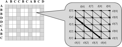
Figure 1: A graphical depiction of the Levenshtein distance dynamic programming grid. On the left, an $x$-partition of the grid. The boundaries of blocks are shaded in gray. On the right, the $DIST$ table corresponding to the upper-rightmost block in the partition. The substrings corresponding to this block are “ABCD” in $A$, and “ABBD” in $B$.

We will work with sub-grids of the dynamic programming grid that will be referred to as blocks. The input vertices of a block are all vertices in the first row and column of the block, while its output vertices are all vertices in the last row and column. Together, the input and output vertices are referred to as the boundary of the block. The substrings of $A$ and $B$ associated with a block are defined in the straightforward manner according to its first row and column. Also, for convenience purposes, we will order the input and output vertices, with both orderings starting from the vertex in bottom-leftmost corner of the block, and ending at the vertex in the upper-rightmost corner. The $i$th input vertex and $j$th output vertex are the $i$th and $j$th vertices in these orderings as depicted in Fig. 1.

Definition 1 ($x$-partition)

Given a positive integer $x\leq N$, an $x$-partition of $G$ is a partitioning of $G$ into disjoint blocks such that every block has boundary of size $O(x)$, and there are $O(N/x)$ blocks in each row and column.

The central dynamic programming tool used by the block edit-distance algorithm is the $DIST$ table, an elegant and handy data structure which was originally introduced by Apostolico et al. [4], and then further developed by others in [10, 29] (see Fig. 1).

Definition 2 ($DIST$ [4])

Let $G^{\prime}$ be a block in $G$ with $x$ input vertices and $x$ output vertices. The $O(x^{2})$ DIST table corresponding to $G^{\prime}$ is an $x\times x$ matrix, with $DIST[i,j]$ storing the weight of the minimum weight path from the $i$th input to the $j$th output in $G$, and $\infty$ if no such paths exists.

In the case of rational scoring functions, Schmidt [29] was the first to identify that the $DIST$ table can be succinctly represented using $O(x)$ space, at a small cost to query access time. In [29] the author took advantage of the fact that the number of relevant changes from one column to the next in the $DIST$ matrix is constant. Therefore, the $DIST$ matrix can be fully represented using only the $O(x)$ relevant points, which requires only $O(x)$ space.

Definition 3 (Succinct $DIST$ [29])

A succinct representation of an $x\times x$ $DIST$ table is a data structure requiring $O(x)$ space, where the value $DIST[i,j]$, given any $i,j\in\{1,\ldots,x\}$, can be queried in $O(\log^{2}x)$ time.

It is important to notice that the values at the output vertices of a block are completely determined by the values at its input and its corresponding $DIST$ table. In particular, if $I[i]$ and $O[j]$ are the values at the $i$th input vertex and $j$th output vertex of a block $G^{\prime}$ of $G$, then

$$O[j]=\min_{1\leq i\leq x}(I[i]+DIST[i,j]).$$ (2)

By (2), the values at the output vertices of $G^{\prime}$ are given by the column minima of the matrix $I+DIST$. Furthermore, by a simple modification of all $\infty$ values in $I+DIST$, we get what is known as a totally monotone matrix [10]. Aggarwal et al. [1] gave an elegant recursive algorithm, nicknamed SMAWK in the literature, that computes all column minima of an $x\times x$ totally monotone matrix by querying only $O(x)$ elements of the matrix. It follows that using SMAWK we can compute the output values of $G^{\prime}$ in $O(x)$ time. We will be using this mechanism for the arbitrary scoring function. However, for the case of rational scoring functions, using SMAWK on the succinct representation of $DIST$ requires $O(x\log^{2}x)$ time. Tiskin [33] showed how to reduce this to $O(x\log x)$ using a simple divide-and-conquer approach.

In addition, let us now discuss how to efficiently construct the $DIST$ table corresponding to a block in $G$. Observe that this can be done quite easily in $O(x^{3})$ time, for blocks with boundary size $O(x)$, by computing the standard dynamic programming table between every prefix of $A$ against $B$ and every prefix of $B$ against $A$. Each of these dynamic programming tables contains all values of a particular row in the $DIST$ table. In [4], Apostolico et al. show an elegant way to reduce the time complexity of this construction to $O(x^{2}\lg x)$. In the case of rational scoring functions, the complexity can be further reduced to $O(x^{2})$ as shown by Schmidt [29].

Block Edit Distance

1. Construct an $x$-partition of the dynamic programming grid of $A$ and $B$, with some $x\leq N$ to be chosen later.

2. Construct a repository with the $DIST$ tables corresponding to each block in the $x$-partition.

3. Fill in the first row and column of $G$ using the standard base case rules.

4. In top-to-bottom and left-to-right manner, identify the next block in the partition of $G$ and use its input and the repository to compute its output using (2). Use the outputs in order to compute the inputs of the next block using (1).

5. The value in the bottom-rightmost cell is the edit distance of $A$ and $B$.

The first two steps of the block edit-distance algorithm are where we actually exploit the repetitive structure of the input strings induced by their SLP representations. These will be explained in further detail in Sections 4 and 5. Apart from these two steps, all details necessary for implementing the block edit-distance algorithm should by now be clear. Indeed, steps 3 and 5 are trivial, and step 4 is computed differently for rational scoring schemes and arbitrary scoring schemes according to the above discussion. Since there are $O(N^{2}/x^{2})$ blocks induced by an $x$-partition, this step requires $O(N^{2}/x)$ time for arbitrary scoring functions, and $O(N^{2}\lg x/x)$ time when dealing with succinct $DIST$ tables in the case of rational scoring functions.

4 Constructing the $\boldmath{x}$-partition

In this section we explain how to construct an $x$-partition of the dynamic programming grid $G$. Each block in this partition, in addition to being associated with a substring $A^{\prime}$ of $A$ and a substring $B^{\prime}$ of $B$, is also associated with unique grammar variables $v\in\mathcal{A}$ and $u\in\mathcal{B}$. It is possible that $A^{\prime}$ is only a prefix or a suffix of the string that is derived from $v$. Similarly, it is possible that $B^{\prime}$ is only a prefix or a suffix of the string that is derived from $u$. However, every pair of grammar variables $(v\in\mathcal{A},u\in\mathcal{B})$ is only associated with one pair of substrings $(A^{\prime},B^{\prime})$. Notice that in the $x$-partition, it is possible that more than one block is associated with substrings $(A^{\prime},B^{\prime})$. This is due to the inherent repetitions in the parse tree that are crucial for the efficiency of our algorithm.

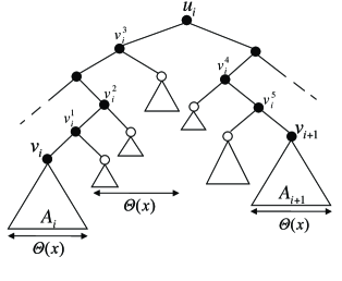
The key-vertices $v_{i}$ and $v_{i+1}$ both derive strings of length $\Theta(x)$, and their least common ancestor is $u_{i}$. The white vertices “hanging” off the $v_{i}$-to-$v_{i+1}$ path are variables that together derive the substrings yet to be covered. Notice that the white vertices derive strings of length shorter than $x$. In the final partition, $v_{i}^{3}$ is associated with an actual substring in the partition. $v_{i}^{2}$ is associated with a prefix of this substring.

Figure 2: A closer look on the parse tree of an SLP $\mathcal{A}$.

To describe the $x$-partition procedure, we explain how $A$ is partitioned into substrings, $B$ is partitioned similarly. We show that for every SLP $\mathcal{A}$ generating a string $A$ and every $x\leq N$, one can partition $A$ into $O(N/x)$ disjoint substrings, each of length $O(x)$, such that every substring is the complete or partial generation of some variable in $\mathcal{A}$. The outline of the partition process is as follows:

1. We first identify the grammar variables in $\mathcal{A}$ which generate a disjoint substring of length between $x$ and $2x$. There are at most $O(N/x)$ such variables.

2. We then show that the substrings of $A$ that are still not associated with a variable can each be generated by $O(N/x)$ additional variables. Furthermore, while, these additional $O(N/x)$ variables may generate a string of length greater than $x$, we will show how to extract only the desired substring from the string that they generate. We add all such variables to our partition of $A$ for a total of $O(N/x)$ variables.

To clarify, lets look at the example depicted in Fig. 2. In step 1 described above, the vertexes $v_{i}$ and $v_{i+1}$ are selected. In step 2, vertices $v_{i}^{3}$ and $v_{i}^{4}$ are selected. For the latter, we will use only a portion of the strings generated by these variables as needed by the algorithm.

We now give a detailed description of the partition process. To partition $A$, consider the parse tree of $\mathcal{A}$ as depicted in Fig. 2. We begin by assigning every grammar variable (vertex) that derives a string shorter than $x$ with the exact string that it derives. We continue by marking every vertex $v$ that derives a string of length greater than $x$ as a key-vertex iff both children of $v$ derive strings of length smaller than $x$. This gives us $O(N/x)$ key-vertices, such that each derives a string of length $\Theta(x)$. We then partition $A$ according to these vertices. In particular, we associate each key-vertex with the exact string that it derives. But we are still not guaranteed that the key-vertices cover $A$ entirely.

To fix this, we take a look at two key-vertices $v_{i},v_{i+1}$ selected in the above process as seen in Fig. 2. Assume $v_{i}$ derives the string $A_{i}$ and $v_{i+1}$ derives the string $A_{i+1}$, and that $A^{\prime}_{i}$ is the “missing” substring of $A$ that lies between $A_{i}$ and $A_{i+1}$. Note that both $A_{i}$ and $A_{i+1}$ are of length $\Theta(x)$, $A^{\prime}_{i}$ however, can be either longer than $\Theta(x)$ or shorter. We now go on to show how to partition $A^{\prime}_{i}$ into $O(|A^{\prime}_{i}|/x)$ substrings of length $O(x)$ each.

Let $u_{i}$ be the lowest common ancestor of $v_{i}$ and $v_{i+1}$, and let $v_{i}^{1},\ldots,v_{i}^{s}$ (resp. $v_{i}^{s+1},\ldots,v_{i}^{t}$) be the vertices, not including $u_{i}$, on the unique $v_{i}$-to-$u_{i}$ (resp. $u_{i}$-to-$v_{i+1}$) path whose right (resp. left) child is also on the path. We focus on partitioning the substring of $A^{\prime}_{i}$ corresponding to the $v_{i}$-to-$u_{i}$ path (partitioning the $u_{i}$-to-$v_{i+1}$ part is done symmetrically). The following procedure partitions this part of $A^{\prime}_{i}$ and associates every one of $v_{i}^{1},v_{i}^{2},\ldots,v_{i}^{s}$ with a substring.

1. initialize $j=1$

2. while $j\leq s$

3. associate $v_{i}^{j}$ with the string derived by its right child, and initialize $S$ to be this substring

4. while $|S|<x$ and $j\neq s$

5. concatenate the string derived by $v_{i}^{j+1}$’s right child to $S$

6. associate the new $S$ with $v_{i}^{j+1}$

7. $j\leftarrow j+1$

8. set $S$ as a string in the $x$-partition

It is easy to verify that the above procedure partitions $A^{\prime}_{i}$ into $O(|A^{\prime}_{i}|/x$) substrings, where one substring can be shorter than $x$ and all the others are of length between $x$ and $2x$. Therefore, after applying this procedure to all $A^{\prime}_{i}$s, $A$ is partitioned into $O(N/x)$ substrings each of length $O(x)$. It is also easy to see that we can identify the key-vertices, as well as the $v_{i}^{j}$ vertices in $O(N)$ time.

An important observation that we point out is that the basic structure of an SLP grammar constitutes that every internal node in the tree represents a variable in the grammar and a grammar variable of the form $v_{i}^{j}$ is always associated with the same substring $S$ (and $|S|\leq 2x$). Due to the bottom-up nature of the above process, the same respective key-vertices in the subtree of a given variable, will be chosen for any appearance of that variable in the tree. This is because in every place in the parse tree where $v_{i}^{j}$ appears, the subtree rooted at $v_{i}^{j}$ is exactly the same, so the above (bottom-up) procedure would behave the same.

5 Constructing the $\boldmath{DIST}$ Repository

In the previous section, we have seen how to construct an $x$-partition of the dynamic programming grid $G$. Once this partition has been built, the first step of the block edit-distance procedure is to construct a repository of $DIST$ tables corresponding to each block of the partition. In this section we discuss how to construct this repository of $DIST$ tables efficiently.

We will be building the $DIST$ tables by utilizing the process of merging two $DIST$ tables. That is, if $D_{1}$ and $D_{2}$ are two $DIST$ tables, one between a pair of substrings $A^{\prime}$ and $B^{\prime}$ and the other between $A^{\prime}$ and $B^{\prime\prime}$, then we refer to the $DIST$ table between $A^{\prime}$ and $B^{\prime}B^{\prime\prime}$ as the product of merging $D_{1}$ and $D_{2}$. For an arbitrary scoring function, merging two $x\times x$ $DIST$ tables requires $O(x^{2})$ time using $x$ iterations of the SMAWK algorithm discussed in Section 3. For the rational scoring function, a recent important result of Tiskin [33] shows how using the succinct representation of $DIST$ tables, two $DIST$ tables can be merged in $O(x\lg x)$ time.

Recall that the $x$-partitioning step described in Section 4 associates SLP variables with substrings in $A$ and $B$. Each substring which is associated with a variable is of length $O(x)$. There are two types of associated substrings: Those whose associated SLP variable derives them exactly, and those whose associated variable derives a superstring of them. As a first step, we construct the $DIST$ tables between any pair of substrings $A^{\prime}$ and $B^{\prime}$ in $A$ and $B$ that are associated with a pair of SLP variables, and are of the first type. This is done in a recursive manner. We first construct the four $DIST$ tables that correspond to the pairs $(A^{\prime}_{1},B^{\prime}_{1})$, $(A^{\prime}_{1},B^{\prime}_{2})$, $(A^{\prime}_{2},B^{\prime}_{1})$, and $(A^{\prime}_{2},B^{\prime}_{1})$, where $A^{\prime}_{1}$ and $A^{\prime}_{2}$ (resp. $B^{\prime}_{1}$ and $B^{\prime}_{2}$) are the strings derived by the left and right children of $A^{\prime}$’s (resp. $B^{\prime}$’s) associated variable. We then merge these four $DIST$s together to obtain a $DIST$ between $A^{\prime}$ and $B^{\prime}$.

Now assume $A^{\prime}$ is a substring in $A$ of the second type, and we want to construct the $DIST$ between $A^{\prime}$ and a substring $B^{\prime}$ in $B$. For simplicity assume that $B^{\prime}$ is a substring of the first type. Then, the variable associated with $A^{\prime}$ is a variable of the form $v^{j}_{i}$ on a path between some two key vertices $v_{i}$ and $v_{i+1}$. For each $k\leq j$, let $A^{k}_{i}$ denote the substring associated with $v^{k}_{i}$. Notice that $A^{\prime}$ is the concatenation of $A^{j-1}_{i}$ and the substring $A^{\prime\prime}$ that is derived from $v^{j}_{i}$’s right child. The $DIST$ between $A^{\prime}$ and $B^{\prime}$ is thus constructed by first recursively constructing the $DIST$ between $A^{j-1}_{i}$ and $B^{\prime}$, and then merging this with the $DIST$ between $A^{\prime\prime}$ and $B^{\prime}$. The latter already being available since the variables associated with $A^{\prime\prime}$ and $B^{\prime}$ are of the first type.

Lemma 1

Building the $DIST$ repository under a rational scoring function can be done in $O(n^{2}x\lg x)$ time.

Proof

Recall that for rational scoring functions, merging two succinct $DIST$s of size $O(x)$ each requires $O(x\lg x)$ time [33]. We perform exactly one merge per each distinct pair of substrings in $A$ and $B$ induced by the $x$-partition. Since each substring is associated with a unique SLP variable, there can only be $O(n^{2})$ distinct substring pairs. Thus, we get that only $O(n^{2})$ merges of succinct $DIST$s need to be performed to create our repository, hence we achieve the required bound. ∎

Lemma 2

Building the $DIST$ repository under an arbitrary scoring function can be done in $O(n^{2}x^{2})$ time.

Proof

In the case of arbitrary scoring functions, merging two $x\times x$ $DIST$ tables requires $O(x^{2})$ time. The same upper bound shown above of $O(n^{2})$ merges may be performed in this case as well, and therefore we achieve the required bound. ∎

6 Putting It All Together

As the major components of our algorithms have now been explained, we go on to summarize our main results. In particular, we complete the proof of Theorem 1.1 and 1.2.

Lemma 3

The block edit distance algorithm runs in $O(n^{2}x\lg x+N^{2}\lg x/x)$ time in case the underlying scoring function is rational.

Proof

The time required by the block edit-distance algorithm is dominated by computing the repository of $DIST$ tables in step 2, and the cost of computing the output values of each block in step 4. Steps 1,3 and 5 all take linear time or less. As we have shown in Section 5, in case the underlying scoring function is rational, the $DIST$ table repository can be built in $O(n^{2}x\lg x)$ time, accounting for the first component of our bound. As explained in Section 3, step 4 of the algorithm requires $O(N^{2}\lg x/x)$ time, accounting for the second component in the above bound. ∎

To conclude, constructing an $x$-partition with $x=N/n$, we get a time complexity of $O(nN\lg(N/n))$, proving Theorem 1.1.

Lemma 4

The block edit distance algorithm runs in $O(n^{2}x^{2}+N^{2}/x)$ time in case the underlying scoring function is arbitrary.

Proof

As described above, the time required by our algorithm is dominated by computing the repository of $DIST$ tables in step 2, and the cost of propagating the dynamic programming values through block boundaries in step 4. As we have shown in Section 5, in case the underlying scoring function is arbitrary, the repository of $DIST$ tables can be built in $O(n^{2}x^{2})$ time, accounting for the first component of our bound. As explained in Section 3, step 3 requires $O(N^{2}/x)$ time, therefore completing the proof of the above bound. ∎

To conclude, constructing an $x$-partition with $x=(N/n)^{2/3}$, we get a time complexity of $O(n^{2/3}N^{4/3})$, proving Theorem 1.2.

References

- [1] A. Aggarwal, M.M. Klawe, S. Moran, P. Shor, and R. Wilber. Geometric applications of a matrix-searching algorithm. Algorithmica, 2:195–208, 1987.
- [2] A. Amir, G. Benson, and M. Farach. Let sleeping files lie: Pattern matching in Z-compressed files. Journal of Computer and System Sciences, 52(2):299–307, 1996.
- [3] A. Amir, G.M. Landau, and D. Sokol. Inplace 2d matching in compressed images. In Proc. of the 14th annual ACM-SIAM Symposium On Discrete Algorithms, (SODA), pages 853–862, 2003.
- [4] A. Apostolico, M.J. Atallah, L.L. Larmore, and S.McFaddin. Efficient parallel algorithms for string editing and related problems. SIAM Journal on Computing, 19(5):968–988, 1990.
- [5] A. Apostolico, G.M. Landau, and S. Skiena. Matching for run length encoded strings. Journal of Complexity, 15(1):4–16, 1999.
- [6] O. Arbell, G. M. Landau, and J. Mitchell. Edit distance of run-length encoded strings. Information Processing Letters, 83(6):307–314, 2001.
- [7] P. Bille and M. Farach-Colton. Fast and compact regular expression matching. Theoretical Computer Science, 302(1-3):211–222, 2003.
- [8] H. Bunke and J. Csirik. An improved algorithm for computing the edit distance of run length coded strings. Information Processing Letters, 54:93–96, 1995.
- [9] P. Cégielski, I. Guessarian, Y. Lifshits, and Y. Matiyasevich. Window subsequence problems for compressed texts. In Proc. of the 1st symp. on Computer Science in Russia (CSR), pages 127–136, 2006.
- [10] M. Crochemore, G.M. Landau, and M. Ziv-Ukelson. A subquadratic sequence alignment algorithm for unrestricted scoring matrices. SIAM Journal on Computing, 32:1654–1673, 2003.
- [11] D. Gusfield. Algorithms on Strings, Trees, and Sequences. Computer Science and Computational Biology. Cambridge University Press, 1997.
- [12] D. Hermelin, S. Landau, G.M. Landau, and O. Weimann. A unified algorithm for accelerating edit-distance via text-compression. In Proc. of the 26th International Symposium on Theoretical Aspects of Computer Science (STACS), pages 529–540, 2009.
- [13] J. Karkkainen, G. Navarro, and E. Ukkonen. Approximate string matching over Ziv-Lempel compressed text. In Proc. of the 11th symposium on Combinatorial Pattern Matching (CPM), pages 195–209, 2000.
- [14] J. Karkkainen and E. Ukkonen. Lempel-Ziv parsing and sublinear-size index structures for string matching. In Proc. of the 3rd South American Workshop on String Processing (WSP), pages 141–155, 1996.
- [15] M. Karpinski, W. Rytter, and A. Shinohara. Pattern-matching for strings with short descriptions. In Proc. of the 6th symposium on Combinatorial Pattern Matching (CPM), pages 205–214, 1995.
- [16] E. Lehman and A. Shelat. Approximation algorithms for grammar-based compression. In Proc. of the 13th annual ACM-SIAM Symposium On Discrete Algorithms, (SODA), pages 205–212, 2002.
- [17] A. Lempel and J. Ziv. Compression of individual sequences via variable-rate coding. IEEE Transactions on Information Theory, 24(5):530–536, 1978.
- [18] A. Lempel and J. Ziv. A universal algorithm for sequential data compression. IEEE Transactions on Information Theory, 409(3):486–496, 2008.
- [19] V.I. Levenshtein. Binary codes capable of correcting deletions, insertions and reversals. Soviet Physics Doklady, 10(8):707–710, 1966.
- [20] Y. Lifshits. Processing compressed texts: A tractability border. In Proc. of the 18th symposium on Combinatorial Pattern Matching (CPM), pages 228–240, 2007.
- [21] Y. Lifshits and M. Lohrey. Querying and embedding compressed texts. In Proc. of the 31st international symposium on Mathematical Foundations of Computer Science (MFCS), pages 681–692, 2006.
- [22] V. Makinen, G. Navarro, and E. Ukkonen. Approximate matching of run-length compressed strings. In Proc. of the 12th Symposium On Combinatorial Pattern Matching (CPM), pages 1–13, 1999.
- [23] U. Manber. A text compression scheme that allows fast searching directly in the compressed file. In Proc of the 5th Symposium On Combinatorial Pattern Matching (CPM), pages 31–49, 1994.
- [24] W.J. Masek and M.S. Paterson. A faster algorithm computing string edit distances. Journal of Computer and System Sciences, 20:18–31, 1980.
- [25] M. Miyazaki, A. Shinohara, and M. Takeda. An improved pattern matching algorithm for strings in terms of straight-line programs. In Proc. of the 8th symposium on Combinatorial Pattern Matching (CPM), pages 1–11, 1997.
- [26] S. Mozes, O. Weimann, and M. Ziv-Ukelson. Speeding up HMM decoding and training by exploiting sequence repetitions. In Proc. of the 18th symposium on Combinatorial Pattern Matching (CPM), pages 4–15, 2007.
- [27] G. Navarro, T. Kida, M. Takeda, A. Shinohara, and S. Arikawa. Faster approximate string matching over compressed text. In Proc. of the 11th Data Compression Conference (DCC), pages 459–468, 2001.
- [28] W. Rytter. Application of Lempel-Ziv factorization to the approximation of grammar-based compression. Theoretical Computer Science, 302(1-3):211–222, 2003.
- [29] J.P. Schmidt. All highest scoring paths in weighted grid graphs and their application to finding all approximate repeats in strings. SIAM Journal on Computing, 27(4):972–992, 1998.
- [30] Y. Shibata, T. Kida, S. Fukamachi, M. Takeda, A. Shinohara, T. Shinohara, and S. Arikawa. Byte Pair encoding: A text compression scheme that accelerates pattern matching. Technical Report DOI-TR-161, Department of Informatics, Kyushu University, 1999.
- [31] Y. Shibata, T. Kida, S. Fukamachi, M. Takeda, A. Shinohara, T. Shinohara, and S. Arikawa. Speeding up pattern matching by text compression. In Proc. of the 4th Italian Conference Algorithms and Complexity (CIAC), pages 306–315, 2000.
- [32] A. Tiskin. Faster subsequence recognition in compressed strings. J. of Mathematical Sciences, to appear.
- [33] A. Tiskin. Fast distance multiplication of unit-monge matrices. In To Appear in Proc. of the 21st annual ACM-SIAM Symposium On Discrete Algorithms, (SODA), 2010.
- [34] R. Wagner and M. Fischer. The string-to-string correction problem. J. of the ACM, 21(1):168–173, 1974.
- [35] J. Ziv and A. Lempel. On the complexity of finite sequences. IEEE Transactions on Information Theory, 22(1):75–81, 1976.
- [36] J. Ziv and A. Lempel. A universal algorithm for sequential data compression. IEEE Transactions on Information Theory, 23(3):337–343, 1977.