Statistical mechanics of Monte Carlo sampling and the sign problem.

Abstract

Monte Carlo sampling of any system may be analyzed in terms of an associated glass model – a variant of the Random Energy Model – with, whenever there is a sign problem, complex fields. This model has three types of phases (liquid, frozen and ‘chaotic’), as is characteristic of glass models with complex parameters. Only the liquid one yields the correct answers for the original problem, and the task is to design the simulation to stay inside it. The statistical convergence of the sampling to the correct expectation values may be studied in these terms, yielding a general lower bound for the computer time as a function of the free energy difference between the true system, and a reference one. In this way, importance-sampling strategies may be optimized.

The sign problem appears when we are asked to compute a partition function of the form:

$$Z=\sum_{s}e^{-W(s)}$$ (1)

and $W=W_{R}+iW_{I}$ is not real. In classical statistical mechanics $s$ denotes a configuration in space and $W=\beta E$ is proportional to the energy, while in the quantum case, $s$ are in space-time and $W$ is the quantum action (and we refer to this as ‘quantum Monte Carlo’). The problem is that a stochastic sampling cannot be performed with the complete $W$, since then the probabilities are no longer positive and real.

An imaginary part of $W$ arises naturally in quantum mechanics with real time, in field theories like QCD with baryons, and in some of the most important systems in condensed matter. In many cases, it is introduced when $W$ is real and of the form $W=W_{o}-b\sum C_{\alpha}^{2}$ and one needs a form linear in the $C_{\alpha}$:

$$Z=\sum_{s}e^{-W_{o}(s)-b\sum C_{\alpha}^{2}}=\sum_{s}\int d{\bf\lambda}\;e^{-W_{o}(s)+\sqrt{b}\lambda_{\alpha}C_{\alpha}-\frac{\lambda_{\alpha}^{2}}{2}}$$

The Hubbard-Stratonovich transformation above introduces an imaginary term $W_{I}=\sqrt{|b|}\sum\lambda_{\alpha}C_{\alpha}$ in the repulsive case $b<0$.

Complex fields: Although the discussion in this paper is general, it is instructive to concentrate on a (very large) class of systems for which the sign problem takes a particularly simple form. They are characterized by having a real action $W_{R}$, plus an imaginary term $W_{I}=ih_{I}M(s)$, where $M(s)$ is an integer-valued function of the configuration, and appear in several contexts:
$\bullet\;\;\;\;$ $\theta$-terms in Euclidean field theories and solid state. $M(s)$ is a topological number associated with the configuration. The case $h_{I}\equiv\theta={i\pi}$, when the partition function is real, is particularly interesting: the term $W_{I}$ may change an otherwise gapped problem into a gapless one (see e.g. Haldane ; Hooft ; W )
$\bullet\;\;\;\;$ Fermion systems such as the Hubbard model

$$H=-t\sum_{<ij>,\sigma}(c^{\dagger}_{i\sigma}c_{j\sigma}+h.c.)+U\sum_{i}n_{i\uparrow}n_{i\downarrow}$$ (2)

The number operators $n_{i\uparrow},n_{i\downarrow}$ may be decoupled with a Hubbard-Stratonovich transformation (either with either continuous or spin Hirsch variables, and the remaining determinants evaluated. When the model is repulsive, these determinants pick up a minus sign counting fermion world-line crossings Loh , and in some cases $M(s)$ can be shown to be a topological number related to the Hubbard Stratonovich field $s$ Mura .
$\bullet\;\;\;\;$ An alternative strategy to uncouple the number operators introduced by DeForcrand and Batrouni Batrouni uses a modified uncoupling with spins, and then $M(s)$ is the sum over space and time of the number of ”up” spins.

In all these cases the sign problem arises because we have to calculate a partition function

$$Z = \sum_{M}\;Z_{M}\;e^{-ih_{I}M}$$ (3)

$$Z_{M} = e^{-\beta F(M)}=\sum_{s}\;\delta(M(s)-M)\;e^{-W_{R}}$$ (4)

with $F(M)$ a real, extensive quantity that may be computed with standard Monte Carlo. This is a deceptively simple expression, since the sum (3) contains detailed cancellations that require an enormous precision in the $F(M)$.

Sampling: In the presence of sign problem, the alternative is to use only the real part in the Monte Carlo rule, and evaluate the expectation of a function $O$ as:

$$\langle O\rangle=\frac{\langle e^{-iW_{I}}\;O\rangle_{\mbox{\tiny R}}}{\langle e^{-iW_{I}}\rangle_{\mbox{\tiny R}}}$$ (5)

where $\langle\bullet\rangle_{\mbox{\tiny R}}$ denotes an average evaluated with the Boltzmann weight of the real part $W_{R}$, a quantity easily calculable with Monte Carlo sampling. Somewhat more generally, we may apply reweighting,

$$\langle O\rangle=\frac{\langle e^{-A-iW_{I}}\;O\rangle_{\mbox{\tiny A}}}{\langle e^{-A-iW_{I}}\rangle_{\mbox{\tiny A}}}$$ (6)

where the average $\langle\bullet\rangle_{\mbox{\tiny A}}$ is associated with the energy $-A+W_{R}$, involving the suitably chosen importance sampling function $A$. In practice, these expectation values are generated by running a Monte Carlo program with energy $-A+W_{R}$ for a time ${\cal{T}}$. If the correlation time of the Monte Carlo dynamics is $\tau$, this is essentially like using $R$ independent samplings: $R={\cal{T}}/\tau$ , which we parametrize as $R=e^{\gamma N}$.

We may restate the problem as follows: we are given $R=e^{\gamma N}$ configurations $s_{a}=\{s_{1},...,s_{R}\}$, chosen independently with probability

$$P(s)=\frac{e^{A(s)-W_{R}(s)}}{\sum_{s^{\prime}}e^{A(s^{\prime})-W_{R}(s^{\prime})}}$$ (7)

where the sum in the denominator runs over all possible values the configuration $s^{\prime}$ my take. We estimate averages (6) as:

$$\langle O\rangle_{estd.}=\frac{\sum_{a=1}^{R}e^{-A(s_{a})-iW_{I}(s_{a})}O(s_{a})}{\sum_{a^{\prime}=1}^{R}e^{-A(s_{a^{\prime}})-iW_{I}(s_{a^{\prime}})}}$$ (8)

which is encoded in the generating (partition) function:

$${\cal{Z}}(j)=\sum_{a=1}^{R}e^{-A(s_{a})-iW_{I}(s_{a})+jO(s_{a})}$$ (9)

Note that we use the same sampled configurations for both numerator and denominator.

Glasses: The connection with glasses arises when we ask: what is the expected result of this procedure? In order to answer this, we need to compute the expectation value of (8), or, equivalently, the expectation of the logarithm of ${\cal{Z}}$: this is a quenched average, a consequence of the random variables appearing in both numerator and denominator of (8). We calculate then:

$$\overline{\ln|{\cal{Z}}(j)|}=\sum_{s_{1},...,s_{R}}\;\Pi_{a=1}^{R}\;P(s_{a})\;\;{\ln|{\cal{Z}}_{j}}(s_{1},...,s_{R})|$$ (10)

Real and imaginary parts of expectation values are obtained from:

$$\langle O\rangle_{estd}=\left.\left(\frac{\partial}{\partial j_{R}}-i\frac{\partial}{\partial j_{I}}\right)\;\overline{\ln|{\cal{Z}}(j)|}\right|_{j=0}$$ (11)

We have chosen to express everything in terms of the average of the logarithm of the norm of the partition function, because its phase in general fluctuates from realization to realization  Derrida1 ; Moukarzel . Equations (7) and (9) define a disordered system, a generalization of the Random Energy Model Derrida2 . The quantity ${\ln|{\cal{Z}}(j)|}$ is self-averaging in the thermodynamic limit. The result contains, as we shall see, different phases, depending on the parameters of the original problem and on the number of samples $e^{\gamma N}$ : $\gamma$ is now a phase parameter. Of these phases of the glassy model, only one coincides with the original model, the others give – even as $N\rightarrow\infty$ – wrong results for the sampling. Monte Carlo sampling in the presence of the sign problem may be understood as the art of being in the only ‘good’ phase.

For clarity of presentation, we shall now specialize to the situation described by complex fields (3) and (4), and then mention how to proceed generally. We collect a number of samples $R$, classify them with their value $M$, obtained with probability $P(M)$. The result is a set of ${\cal{N}}(M)$ , with $\sum_{M}{\cal{N}}(M)=R=e^{N\gamma}$. Expectation values are obtained from (cfr. (8)):

$$\langle O\rangle_{estd}=\frac{\sum_{M}{\cal{N}}(M)e^{ih_{i}M}O(M)}{\sum_{M^{\prime}}{\cal{N}}(M^{\prime})e^{ih_{i}M^{\prime}}}$$ (12)

The ${\cal{N}}$ are random variables, and we wish to calculate the expected result for (12). We recognize a form of the Random Energy Model (REM) with imaginary inverse temperature $h_{I}$, and $M$ playing the role of energy. The input from the original system is through the (real) free energy densities $F(M)$, for real $M$, the quantity we estimate through our simulation. (The usual REM corresponds to a quadratic $F(M)$). The solution of this problem follows closely refs. Derrida1 ; Moukarzel .

For large $N$, because of independence, one can convince oneself that

$$\langle({\cal{N}}(M)-\langle{\cal{N}}(M)\rangle)^{2}\rangle\sim\langle{\cal{N}}(M)\rangle\sim\;R\;P(M)$$ (13)

We have that either $R\;P(M)\ll 1$, and there are no samples of that value of $M$, or $R\;P(M)\gg 1$. In the latter case, one has that the average number of samples of given $M$ is ${\cal{N}}{(M)}\sim RP(M)$, but with an error $\sqrt{{\cal{N}}{(M)}}$, where:

$$P(M)=\frac{e^{-\beta F(M)}}{\sum_{M^{\prime}}e^{-\beta F(M^{\prime})}}{\;\sim\;}e^{-\beta N[f(m)-f(m_{o})]}$$ (14)

For convenience we have defined the intensive quantities $f(m=M/N)=F(M)/N$. The term with $f(m_{o})$ comes from the normalization integral $\int dme^{-\beta f(m)}$, and $m_{o}$ is the real axis saddle $\frac{df}{dm}\;(m_{o})=0$.

In order to calculate the result of (12) we start with the partition function:

$${\cal{Z}}=\sum_{M}\;\;{\cal{N}}(M)e^{-ih_{I}M}$$ (15)

Writing ${\cal{N}}\sim{R}P(M)+{R^{\frac{1}{2}}}P^{\frac{1}{2}}(M)\eta(M)$, where $\eta(M)$ is a random number of zero mean and unit variance, we may split $\cal Z$ into a deterministic ${{\cal{Z}}}_{det}$ plus a fluctuating part ${\cal{Z}}_{err}$. The deterministic part reads:

$${{\cal{Z}}}_{det} = {\sum_{M}\;RP(M)e^{-ih_{I}M}}$$ (16)

$${\;\sim\;} \int dm\;e^{N[{\gamma}-\beta f(m)+\beta f(m_{o})-ih_{I}m]}$$

The integral (16) is dominated by the saddle point

$${\beta}\frac{df}{dm}(m_{sp}){+}ih_{I}=0$$ (17)

Note that, unlike the real-axis saddle $m_{o}$, the total one $m_{sp}$ is complex. This is the correct solution, and we shall denote it ‘ Phase I’.

The shifting of the correct saddle point into the complex plane is due to the rapid oscillations introduced by the imaginary term, which have the effect of making the final result no longer dominated by the envelope maximum at $m_{o}$ – and indeed, the final result is exponentially smaller than the peak $e^{-N\beta f(m_{o})}$. In the case of our sampling, this means that we should also consider two effects, each one leading to a new phase: The first is the fact that for values of $m$ distant enough from the maximum, the sampling produces no configurations at all. The region of integration is restricted to values $m$ bounded by the points $m_{b}$ such that ${\cal{N}}{(M)}=e^{-\beta N[f(m_{b})-f(m_{o})]}R\stackrel{{\scriptstyle>}}{{~{}}}1$, that is, within the limits given by:

$$\beta[f(m_{b})-f(m_{o})]=\gamma$$ (18)

The second effect comes from the fact that our integrand is noisy: this is particularly serious because the correct result depends upon very strict cancellations giving an exponentially smaller answer. The error due to the noise of the integrand is:

$${\cal{Z}}_{err} = \int dm\;\sqrt{{\cal{N}}(M)}e^{-Nih_{I}m}\;\eta(m)$$

$${\;\sim\;} e^{{+}\frac{N\gamma}{2}}\int dm\;e^{-N[\beta(f(m)-\beta f(m_{o}))/2+ih_{I}m]}\;\eta(m)$$

This is a fluctuating quantity. The expectation of $|{\cal{Z}}_{err}|^{2}$ over noise is easy to evaluate by saddle point, using $\langle\eta(m)\eta(m^{\prime})\rangle\sim\delta(m-m^{\prime})$, and one gets that:

$$|{\cal{Z}}_{err}|\sim e^{\frac{\gamma{N}}{2}}$$ (19)

All in all, there are three types of phases Derrida1 ; Moukarzel , a charateristic feature of glassy systems with complex parameters:
$\bullet\;\;\;$ Phase I: The correct sampling of the original system, (up to usual finite-size effects). Here it appears as a ‘liquid’ phase of the glass, dominated by a saddle point $m_{sp}$ that is outside the domain of integration of (17), either because $m_{sp}$ is complex, or because it is real but beyond the original interval.
$\bullet\;\;\;$ Phase II: A ‘frozen’ phase, where the solution is dominated by one of the boundaries in sampling $m_{b}$ satisfying (18).
$\bullet\;\;\;$  Phase III: An ‘chaotic’ phase: the sampling noise destroys the cancellations brought about by the oscillatory terms, and the peak of the ‘envelope’ of the integrand dominates. This phase can be shown to contain a surface density of Lee-Yang zeroes in the complex plane Derrida1 ; Moukarzel .

In the present case, with $A=0$, phase II never dominates. The boundary between Phases I and III is given by the line where the two real parts of the free energies coincide and when the contour deformation over the integral (16) passes through the saddle. Then, in order to be in the Phase I, we need

$${h_{I}\max{(m_{b})}>{\mbox{Im}}[\beta f(m_{sp})+ih_{I}m_{sp}]>h_{I}\min{(m_{b})}}$$

(20)

$$-[{\mbox{Re}}[\beta f(m_{sp})+{ih_{I}m_{sp}}]-\beta f(m_{o})]+\frac{\gamma}{2}>0$$ (21)

(note that $f(m_{sp})<f(m_{o})$), which may also be written in terms of the free energy at $h_{I}$ and the free energy at $h_{I}=0$. This is the condition for the simulation to yield the good result, which must be read as a bound on the simulation time through the condition that $\gamma$ be large enough. It incorporates the well-known exponential dependence on the inverse temperature, and a free energy difference between the true model and one without the sign problem (i.e. with real field). Note that increasing the system size $N$ at fixed simulation time ${\cal{T}}$ is dangerous, as it implies making $\gamma$ smaller.

Consider next introducing an importance-sampling function of the form $A=Na(m)$. Following the same reasoning as above, we conclude that the free energies differences now become:

$$-\beta(f^{I}-f^{III}) = \beta\frac{f(m_{o}^{+})+f({{m}}_{o}^{-})}{2}+\frac{a(m_{o}^{+})-a({{m}}_{o}^{-})}{2}$$

$$+\frac{\gamma}{2}-\beta f(m_{sp})-{ih_{I}m_{sp}}$$

$$-\beta(f^{I}-f^{II}) = -\beta(f(m_{sp})-f(m_{b}))-{ih_{I}(m_{sp}-m_{b})}$$

where $m_{o}^{+}$ and ${m}_{o}^{-}$ minimize $\beta f(m)\pm a(m)$, respectively, and $m_{b}$ are given by the generalization of (18):

$${\gamma}-\beta(f(m_{b})-f({{m}}_{o}^{{-}}))+a(m_{b})-a({{m}}_{o}^{{-}})=0$$ (22)

Boundaries and free energy differences have changed, and saddle may even be outside the domain of sampling between boundaries. All three phases are possible.

The important point is that this phase structure, and hence the values of $\gamma$ for correct sampling, depends on the free energy of the true system (which we cannot change), and on the free energies $f(m_{o}^{\pm})$, $f(m_{b})$. The latter are properties of the system under real fields, and hence easy to calculate for any $A$. One may then choose the optimal function $A$ that will minimize the $\gamma$ needed to be in phase $I$.

The general case: It is easy to extend the analysis of the disordered model for the general case, in which the imaginary part $W_{I}$ takes an abitrary form. We have to express free energies and probabilities in terms of three collective variables $W_{I}$ and $A$, playing the role of $M$. The probability of a pair ($W_{I},A$) is :

$$P(W_{I},A)\propto\sum_{s}\;e^{A(s)-W_{R}(s)}\delta(W_{I}(s)-W(I))\delta(A(s)-A)$$

and we use it to compute the average of $\ln|{\cal{Z}}(W_{I},A)|$. There may be again three phases, depending on whether what dominates is a saddle point of complex ($W_{I},A$), the boundary in the ($W_{I},A$)-plane where there is sampling, or the incoherent noise. The frontiers of these phases depend on number of samples through $\gamma$, and also on the choice of importance sampling function $A$.

The Lee-Yang zeroes: At the Lee-Yang zeroes of the original problem (i..e. Phase I), $Z=0$ and $f\rightarrow\infty$. It may seem that these are then problematic regions for sampling. Actually, this is not really so. The reason is as follows: in the large $N$ limit, Lee-Yang zeroes appear when two solutions compete:

$$Z\sim e^{-N[f_{R}^{1}+if_{I}^{1}](h)}+e^{-N[f_{R}^{2}+if_{I}^{2}](h)}$$ (23)

(note that here we are using the Legendre-transformed free energy, in terms of $h$). Along the transition line in the complex plane where $f_{R}^{1}(h)=f_{R}^{2}(h)=f_{R}(h)$, the partition function is $Z\sim e^{-Nf_{R}(h)}[e^{iNf_{I}^{1}(h)}-e^{iNf_{I}^{2}(h)}]$, and zeroes occur where the oscillating factors cancel. In order for the oscillating factor to be of the same order as $Nf_{R}(h)$, the factor $[e^{iNf_{I}^{1}(h)}-e^{iNf_{I}^{2}(h)}]$ has to be exponentially small in $N$, and this happens only very close to each zero. We conclude that each zero has a very small region of influence in which the partition function is really small.

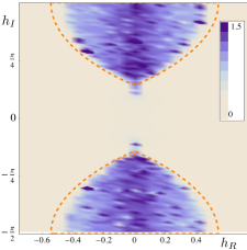
Figure 1: Simulated minus exact value of the magnetization in terms of the complex fields $h$ for $\gamma=0.5$, $J=0.5$ and $N=100$. The boundary between phases I and III is indicated with a dashed line determined through (21).

An example: ferromagnet in a complex field: Let us consider, as a simple example, a mean-field Ising ferromagnet under a complex field $h=h_{R}+ih_{I}$. We have that $Z=e^{-N\beta f(m)-ih_{I}mN}$, with:

$$-\beta f(m) = {-\frac{1}{2}(1+m)\ln(1+m)-\frac{1}{2}(1-m)\ln(1-m)}$$ (24)

$${+\frac{\beta J}{2}m^{2}-h_{R}m}$$

The correct solution of the problem is given by the saddle point equation $m_{sp}=\tanh(\beta Jm_{sp}+h)$

For complex $h$, in general $m_{sp}$ will be complex, except for $h_{I}=\frac{\pi}{2}$, where it will be real but outside the interval $[-1,1]$.

Figure 1 shows the sampled magnetization (subtracting, for clarity, the exact value) in terms of the field $h$, with a fixed sampling time $e^{N\gamma}$. In Figure 2 we show the frontier in detail, with the regions in Phase I surrounding the lee-Yang zeroes. Clearly the size of the islands decreases for larger systems.

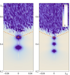
Figure 2: A detail of the frontier between phases I and III under the same conditions of Figure 1 with $N=60$ (left) and $N=100$ (right). The islands visible within phase I (correct sampling) are the neighborhoods of Lee-Yang zeroes of the ferromagnet

Conclusions: We have shown that the error brought about by the sign problem may be discussed in terms of the statistical mechanics of a glass model at complex fields. A first suggestion of this analysis is that simulations should be characterized by the size $N$ and $\gamma=\frac{\ln{\cal T}}{N}$, where ${\cal T}$ is the time. A first simulation with relatively modest values of $N$ may be used to obtain the boundary $\gamma_{c}$ of phase $I$, and only then embark on larger sizes, with times determined by fixed $\gamma\stackrel{{\scriptstyle>}}{{\sim}}\gamma_{c}$.

A more sophisticated strategy is to approach the desired parameter (say, $h_{I}=\pi$) gradually, from smaller $h_{I}$, and estimate $\gamma_{c}(h_{I})$. Because the sign problem is less severe for smaller values of $h_{I}$, one may reach the desired situation by a succession of correctly sampled problems.

As mentioned above, all importance sampling strategies work by increasing the free energy of phases II and III, thus making phase I more favorable at given value of $\gamma$. Because of the nature of these phases, this may be optimized on the basis of the knowledge of the free energy of the system at real fields alone.

To conclude, let us mention that an analysis very similar to the one made here may be applied to the numerical implementation of analytic continuation.

References

- (1) F.D.M. Haldane, Phys. Let 93A (1983) 464;I. Affleck, Nucl. Phys. B257 (1985) 397.
- (2) G. t’Hooft, Nucl. Phys. B190 (1981) 455.
- (3) J.E. Hirsch, Phys. Rev. B 28, 4059
- (4) E.Y. Loh, J.E. Gubernatis, R.T. Scaletar, S.R. White, D.J. Scalapino and R.L. Sugar, Phys. Rev. B41 9301 (1990).
- (5) A. Muramatsu, G. Zumbach and X. Zotos, International Journal of Modern Physics C3 185 (1992).
- (6) Batrouni GG, de Forcrand P., Phys Rev B Condens Matter. 48(1993) 589
- (7) Derrida B., Physica A 177 (1991) 31
- (8) C. Moukarzel and N. Parga: Physica A 177 (1991) 24; J. Phys. I France 2 (1992) 251; Physica A 185, (1992) 305
- (9) Derrida B., Phys. Rev. B 24 (1981) 2613; Phys. Rep. 67 (1980) 29.
- (10) W. Bietenholz, A. Pochinsky and U. -J. Wiese, Phys. Rev. Lett.75, 4524 (1995)