Anomalous Hall conductivity: local orbitals approach

Abstract

A theory of the anomalous Hall conductivity based on the properties of single site orbitals is presented. Effect of the finite electron life time is modeled by energy fluctuations of atomic-like orbitals. Transition from the ideal Bloch system for which the conductivity is determined by the Berry phase curvatures to the case of strong disorder for which the conductivity becomes dependent on the relaxation time is analyzed. Presented tight-binding model gives by the unified way experimentally observed qualitative features of the anomalous conductivity in the so called good metal regime and that called as bad metal or hopping regime.

I Introduction

It has been known for more than a century that ferromagnetic materials exhibit, in addition to the standard Hall effect when placed in a magnetic field, an extraordinary Hall effect which does not vanish at zero magnetic field. The theory of this so-called anomalous Hall effect has a long and confusing history, with different approaches giving in some cases conflicting results. While more recent calculations have somewhat unified the different approaches and clarified the situation, it is still an active topic of research, see for example the recent review by Nagaosa et al Nagaosa2009 ).

It is generally accepted that anomalous Hall effect is induced by spin-orbit coupling. It was first suggested by Karplus and Luttinger Karplus in 1954 to explain anomalous Hall effect observed on ferromagnetic crystals. Their analysis leads to the scattering independent off-diagonal components of the conductivity, which are attributed to the so-called “intrinsic” effect. Later, theories of this effect based on several specific models have been developed Miyazawa ; Onoda . As shown recently, it is accompanied by a strong orbital Hall effect Shindou ; Kontani_1 . The conductivity is affected by scattering, which in the presence of spin-orbit coupling is basically of two types, the so called side-jump Berger and skew scattering Smit ; Luttinger_58 ; Sinitsyn . They also lead to an anomalous Hall effect, called “extrinsic”. It has also been argued that in the anomalous Hall regime a periodic field of electric dipoles (electric polarizability) is induced by the applied current Karplus ; Adams ; Fivaz . This property has recently been shown to be related to the so-called orbital polarization moment Streda_Jonck which is determined by Berry phase curvature in pure systems Niu .

The best quantitative agreement with experimental observations has been obtained by semi-classical transport theory Niu , leading to the Berry phase correction to the group velocity. For Fe crystals Jungw_2 it yields an anomalous conductivity $\sim 750\;\Omega^{-1}$ cm^-1 while a value approaching $1000\;\Omega^{-1}$ cm^-1 has been observed. However, up to now, generalization of this theory to systems with strong disorder or subject to other types of fluctuations seemed to fail. It is the main aim of this paper to present theoretical treatment filling this gap.

In contrast to standard transport theories the Hall conductivity is expressed in terms of local atomic-like orbitals. It is explicitly derived that for perfect Bloch electron systems this description coincides with that given by Berry phase curvatures indicating intrinsic, topological, origin of anomalous Hall effect. Presented view based on atomic-like orbitals allows to include effect of disorder by a local energy fluctuation of these orbitals which is an alternative description of scattering events. Fluctuations modify the Hall conductivity and transition from perfect to strongly disordered systems is analyzed. So called ”intrinsic” and ”extrinsic” Hall effect are just treated by an unified way. To test presented view based on local atomic-like orbitals the two band model within tight-binding approach is used. Obtained dependence of the anomalous Hall conductivity on the relaxation time shows the observed qualitative features Miyasato . Similar features has also been obtained by the different procedure with relaxation time being a fitting parameter Kontani_2 . In contrast to this work the presented model allows to relate relaxation time to fluctuations of atomic-like orbitals, i.e. to its microscopic origin. By the unified way it gives experimentally observed scaling of anomalous Hall conductivity $\sigma_{xy}$ with diagonal conductivity component $\sigma_{xx}$ in the region of the so called good metal for which $\sigma_{xy}\sim(\sigma_{xx})^{0}$ and that of the bad metal for which $\sigma_{xy}\sim(\sigma_{xx})^{1.6}$.

The paper is organized as follows. In section II basic properties of electron systems in crystalline structures with spin-orbit coupling are summarized, while basic expressions for Hall conductivity derived by using the quantum linear response theory are rederived in the section III. In section IV an alternative expression for Hall conductivity, including on-energy shell matrix elements only, is derived. Section V is devoted to perfect Bloch electron systems where conductivity is expressed in terms of local orbital polarization moments which are further expressed via the Berry phase curvature. In section VI a two-band model in tight-binding approach is presented to estimate the effect of a finite electron life time to the anomalous Hall conductivity at zero magnetic field. Presented theory of anomalous Hall effect is summarized and commented in the last section.

II Single electron Hamiltonian and statistical fluctuations

Within a mean field approach, electron properties are controlled by a single electron Hamiltonian which we consider in the following standard form

$$H\,=\,\frac{\vec{p}^{\;2}}{2m_{0}}\,+\,V(\vec{r})\,+\,\frac{\lambda_{c}^{2}}{4\hbar}\;\vec{\sigma}\cdot\left[\vec{\nabla}V(\vec{r})\,\times\,\vec{p}\,\right]\,+\,$$

$$-\,\mu_{B}\,\vec{B}_{\rm eff}\cdot\vec{\sigma}\;.$$ (1)

Here, $m_{0}$ and $\mu_{B}$ denote free electron mass and the Bohr magneton, respectively, $\vec{p}$ is the momentum operator, $V(\vec{r})$ denotes a background potential and components of $\vec{\sigma}$ are Pauli matrices. The third term on the right hand side represents spin-orbit coupling with $\lambda_{c}$ being an effective Compton length. The last term on the right hand side describes Zeeman-like spin splitting due to the exchange-correlation energy represented by an effective field $\vec{B}_{\rm eff}$ which can generally be position-dependent. The corresponding velocity operator reads

$$\vec{v}\,=\,\frac{1}{i\hbar}\,[\,\vec{r}\,,\,H\,]\,=\,\frac{\vec{p}}{m_{0}}\,+\,\frac{\lambda_{c}^{2}}{4\hbar}\;\vec{\sigma}\times\vec{\nabla}V(\vec{r})\;.$$ (2)

Strictly speaking, Hamiltonian $H$ quite well defines properties of electrons located within a finite volume of characteristic dimensions determined only by the electron coherence length. Within each of such volumes the background potential as well $\vec{B}_{\rm eff}$ can be different. This way, a set of electron systems, the statistical ensemble, is defined. If time-dependent fluctuations can be treated within an adiabatic approach R1_adiabatic_approach , they can also be included in this ensemble. Measurable quantities are given by their statistically averaged values. It is useful to split Hamiltonian $H$, Eq. (II), into two parts

$$H\,=\,H_{0}\,+\,\delta H\qquad,\qquad H_{0}\,\equiv\,\langle H\rangle_{\rm av}\;,$$ (3)

where only $\delta H$ depends on statistical fluctuations. For crystalline solids, to which the present treatment is devoted, statistically averaged Hamiltonian $H_{0}$, obeys full crystal symmetry and the effective field $\vec{B}_{\rm eff}$ can be assumed constant. It defines the so called virtual crystal with eigenstates $|n,\vec{k}\rangle$ of the energy $E_{n}(\vec{k})$, characterized by the band index $n$ and the wave vector $\vec{k}$. Eigenfunctions are two-component Bloch spinors

$$|n,\vec{k}\,\rangle\, = \,\Psi_{n,\vec{k}}(\vec{r})\,=\,\frac{e^{i\vec{k}\vec{r}}}{\sqrt{8\pi^{3}}}\,u_{n,\vec{k}}(\vec{r})\;,$$ (4)

$$H_{0}\,|n,\vec{k}\,\rangle\, \equiv \,\langle H\rangle_{\rm av}\,|n,\vec{k}\,\rangle\,=\,E_{n}(\vec{k})\,|n,\vec{k}\,\rangle\;,$$

where $u_{n,\vec{k}}(\vec{r})$ are spinor functions periodic in $\vec{r}$ with period defined by the elementary lattice translations. Velocity matrix elements are diagonal in the wave vector $\vec{k}$ located within the Brillouin zone

$$\langle n,\vec{k}|\vec{v}\,|n^{\prime},\vec{k}^{\prime}\,\rangle\,=\,\vec{v}^{\;n,n^{\prime}}(\vec{k})\;\delta_{\vec{k},\vec{k}^{\prime}}\;,$$ (5)

and the expectation values read

$$\vec{v}_{n}(\vec{k})\,\equiv\,\langle n,\vec{k}|\vec{v}\,|n,\vec{k}\,\rangle\,=\,\frac{1}{\hbar}\,\vec{\nabla}_{\vec{k}}E_{n}(\vec{k})\;.$$ (6)

Equilibrium properties are determined by the effective Hamiltonian, $H_{\rm eff}$, defined by the statistically averaged Green’s function

$$\langle G(z)\rangle_{\rm av}\,\equiv\,\left\langle\frac{1}{z-H}\right\rangle_{\rm av}\,\equiv\,\frac{1}{z-H_{\rm eff}(z)}\;,$$ (7)

where $z$ is the complex energy variable. It has the full crystal symmetry and it is diagonal in the representation given by eigenstates of the averaged Hamiltonian $H_{0}$, Eq. (4). Effective Hamiltonian is non-Hermitian and energy dependent but it is analytic in both complex half-planes, $H_{\rm eff}(z^{\ast})\,=\,H_{\rm eff}^{+}(z)$. Its standard form reads

$$H_{\rm eff}(z)\,=\,H_{0}\,+\,\Sigma(z)\quad,\quad\Sigma(z)\,=\,\Delta(z)-i\Gamma(z)\;,$$ (8)

where $\Sigma(z)$ is the energy dependent self-energy. Inverse value of its imaginary part represents a finite electron life-time.

To include an external magnetic field $\vec{B}$ the Hamiltonian defined by Eq. (II) has to be modified. Both the momentum operator entering the Hamiltonian, and the velocity operator, Eq. (2), have to be replaced by their counterparts, which include a vector potential $\vec{A}$.

$$\vec{p}\,\rightarrow\,\vec{p}\,+\,e\vec{A}\;.$$ (9)

Here, $e$ denotes the electron charge absolute value and the magnetic field is given as $\vec{B}={\rm curl}\vec{A}$. Also the value of the parameter $\vec{B}_{\rm eff}$ defining Zeeman-like splitting is modified by $\vec{B}$. The external magnetic field generally removes translation symmetry. Exceptions are the so called rational magnetic fields for which the problem becomes invariant under translations with different elementary translations than those given by the periodic potential.

III Linear response theory

In this section the standard linear response theory will be described and well known general formulae derived to summarize basic theoretical assumptions. In accord with the original work by Kubo Kubo the external electric field is supposed to be turned on at the time $t\rightarrow-\infty$ and reach the final value $\vec{\cal{E}}$ at $t=0$. Exponential time evolution is considered, $\vec{\cal{E}}(t)=\vec{\cal{E}}\,e^{\epsilon t/\hbar}$, with $\epsilon>0$ being an infinitesimally small quantity. It gives rise to the Hamiltonian perturbation $e\vec{r}\cdot\vec{\cal{E}}(t)$ and corresponding density matrix ${\bm{\rho}}(t)$ has to satisfy the equation of motion which reads

$$\frac{\partial{\bm{\rho}}(t)}{\partial t}\,+\,\frac{1}{i\hbar}\left[{\bm{\rho}}(t)\,,\,H+e\vec{r}\cdot\vec{\cal{E}}(t)\right]\,=\,0\;.$$ (10)

It can be written in the following way

$${\bm{\rho}}(t)\,=\,{\bm{\rho}}_{0}(H)\,+\,e^{-iHt/\hbar}{\bm{\rho}}_{1}(t)\,e^{iHt/\hbar}\;,$$ (11)

where ${\bm{\rho}}_{1}(t)$ represents the deviation from the density matrix in the absence of electric field given by the Fermi-Dirac distribution function

$${\bm{\rho}}_{0}(H)\,=\,\left(1+e^{\frac{H-\mu}{k_{\rm B}T}}\right)^{-1}\;,$$ (12)

where $\mu$ and $k_{\rm B}T$ are the chemical potential and thermal energy, respectively. Up to linear terms in the electric field, ${\bm{\rho}}_{1}(t)$ reaches the following value at $t=0$

$${\bm{\rho}}_{1}(0)=\frac{i}{\hbar}\int\limits_{0}^{+\infty}e^{-\epsilon t/\hbar}e^{-iHt/\hbar}\left[{\bm{\rho}}_{0}(H)\,,\,e\vec{r}\cdot\vec{\cal{E}}\right]e^{iHt/\hbar}dt\;,$$ (13)

and the resulting current density reads

$$\vec{j}\,=\,-\,e\,\lim_{\epsilon\rightarrow 0^{+}}\left\langle\,{\rm Tr}\left[\,{\bm{\rho}}_{1}(0)\,\vec{v}\,\right]\,\right\rangle_{\rm av}\;.$$ (14)

Generally, the above potential perturbation $e\vec{\cal{E}}\vec{r}$ of the Hamiltonian is not the only perturbation caused by electric field. The potential gradient $e\vec{\cal{E}}$ enters the spin-orbit term of the Hamiltonian, Eq. (II), as well as the velocity operator, Eq. (2), giving rise to additive terms linear in electric field. Resulting contributions to the current density are of a higher order than $\lambda_{c}^{2}$ in the Compton length. For the considered Hamiltonian $H$, Eq. (II), which includes spin-orbit coupling only approximately up to the order of $\lambda_{c}^{2}$, these contributions thus have to be ignored.

Introducing the $\delta$-function operator

$$\delta(\eta-H)=-\lim_{\epsilon\rightarrow 0^{+}}\,\frac{G^{+}(\eta)-G^{-}(\eta)}{2\pi i}\;\;,$$ (15)

$$G^{\pm}(\eta)=\frac{1}{\eta-H\pm i\epsilon}\,,$$

the time integration, Eq. (13), can easily be performed. For the limiting case of the zero temperature in function $\rho_{0}(H)$ the components of the conductivity tensor obey the following form

$$\sigma_{ij}(\mu)\equiv\frac{j_{i}}{{\cal{E}}_{j}}\,=\,\qquad\qquad\qquad$$

$$=-e^{2}\!\!\!\int\limits_{-\infty}^{\mu}\!\!\!\left\langle{\rm Tr}\left\{\delta(\eta-H)\left[v_{i}G^{+}r_{j}+r_{j}G^{-}v_{i}\right]\right\}\right\rangle_{\rm av}\!d\eta\,,$$ (16)

where $i,j=x,y,z$. The proper way to treat the limits in Eqs. (14) (due to the electric field time evolution) and (15) (regularization of $\delta(H-\eta)$) would be to introduce two different infinitesimal parameters and treat both of them independently, after all other steps are taken. However, our procedure of statistical averaging yields a non-zero imaginary part of the self-energy, $\Gamma$, entering both averaged operators, and the limiting case of the fully coherent system is defined by the physically acceptable limit $\Gamma\rightarrow 0^{+}$. That is why it is sufficient to consider just one infinitesimally small parameter $\epsilon\rightarrow 0^{+}$ implicitly entering Eq. (III). Misunderstanding of this limit has been reason for doubts concerning validity of resulting expressions, especially of the Hall conductivity.

The non-zero temperature smearing effect of the distribution function yields

$$\sigma_{ij}(\mu,T)\,=\,-\int\limits_{-\infty}^{+\infty}\frac{d{\bm{\rho}}_{0}(\eta)}{d\eta}\;\sigma_{ij}(\eta)\,d\eta\;.$$ (17)

This relation allows to limit our attention to the analysis of the energy-dependent conductivity given by Eq. (III). It does not mean that $\sigma_{ij}(\mu)$ has to be temperature independent since potential fluctuations as well as some of the Hamiltonian parameters can be implicitly temperature-dependent quantities, as is e. g. $\vec{B}_{\rm eff}$ representing the exchange-interaction effect.

Using definition of the velocity operator

$$\vec{v}\,=\,\frac{1}{i\hbar}\,\left[\vec{r},H\right]=-\frac{1}{i\hbar}\,\left[\vec{r},\left(G^{\pm}(\eta)\right)^{-1}\right]\;,$$ (18)

and the identity

$$\left[G^{\pm}(\eta)\right]^{2}\,=\,-\,\frac{dG^{\pm}}{d\eta}\;,$$ (19)

the Eq. (III) can be rewritten remark_2 in a form including velocity operators only

$$\sigma_{ij}(\mu)=i\hbar e^{2}\times\qquad\qquad\qquad\qquad\qquad\qquad\qquad\quad$$

$$\times\!\!\!\int\limits_{-\infty}^{\mu}\!\!\left\langle{\rm Tr}\left\{\delta(\eta-H)\left[v_{i}\frac{dG^{+}}{d\eta}v_{j}-v_{j}\frac{dG^{-}}{d\eta}v_{i}\right]\right\}\right\rangle_{\rm av}\!\!d\eta\;.\;$$ (20)

It coincides with that obtained by Bastin et al Bastin by the use of a different procedure. For diagonal components of the conductivity tensor the integration by parts gives the well known Kubo-Greenwood formula Greenwood

$$\sigma_{ii}(\mu)\,=\,\pi e^{2}\hbar\left\langle\,{\rm Tr}\left\{v_{i}\delta(\mu-H)v_{i}\delta(\mu-H)\right\}\,\right\rangle_{\rm av}\;.$$ (21)

Making use of the following identity remark_2 ; Smrcka

$$i\hbar{\rm Tr}\left\{\delta(\eta-H)\left[v_{i}\frac{dG^{+}}{d\eta}v_{j}-v_{j}\frac{dG^{-}}{d\eta}v_{i}\right]\right\}\,=\qquad$$

$$=\,\frac{i\hbar}{2}\,\frac{d}{d\eta}\,{\rm Tr}\left\{\delta(\eta-H)\left[v_{i}G^{+}(\eta)v_{j}-v_{j}G^{-}(\eta)v_{i}\right]\right\}\,+$$

$$+\frac{1}{2}\,\frac{d}{d\eta}\,{\rm Tr}\left\{\delta(\eta-H)\left[r_{i}v_{j}-r_{j}v_{i}\right]\right\}\;,\;\;$$ (22)

the off-diagonal conductivity components can be split into two parts Streda_formula

$$\sigma_{xy}(\mu)=\sigma_{xy}^{\rm(I)}(\mu)+\sigma_{xy}^{\rm(II)}(\mu)=-\sigma_{yx}(\mu)\;,$$ (23)

where

$$\sigma_{xy}^{\rm(I)}(\mu)=e^{2}\,\frac{i\hbar}{2}\,\times\hskip 133.72795pt$$

$$\times\left\langle{\rm Tr}\left\{\delta(\mu-H)\left[v_{x}G^{+}(\mu)v_{y}-v_{y}G^{-}(\mu)v_{x}\right]\right\}\right\rangle_{\rm av}\;,$$ (24)

and

$$\sigma_{xy}^{\rm(II)}(\mu)=\frac{e^{2}}{2}\left\langle{\rm Tr}\left\{\delta(\eta-H)\left[xv_{y}-yv_{x}\right]\right\}\right\rangle_{\rm av}\,=$$

$$=\,-e^{2}\left\langle{\rm Tr}\left\{\delta(\eta-H)\,y\,v_{x}\right\}\right\rangle_{\rm av}\;.$$ (25)

These conductivity formulae are quite general, they also include both the effect of the magnetic field and the spin-orbit coupling Bruno . Similar treatment, but formally more complicated Smrcka , is applicable to other transport coefficients, like the thermopower and the heat conductivity.

The above expressions for the Hall conductivity $\sigma_{xy}(\mu)$ have been particularly useful for understanding of the quantum Hall effect. While the contribution $\sigma_{xy}^{\rm(I)}(\mu)$ vanishes whenever $\mu$ is located within an energy gap, the contribution $\sigma_{xy}^{\rm(II)}(\mu)$ can remain finite, giving rise to quantized values of the Hall conductivity Streda_formula . However, these formulae are not very convenient for $\mu$ located within an energy band since, at least for some specific models Streda_84 ; Kontani_2 , a non-negligible part of $\sigma_{xy}^{\rm(I)}(\mu)$ is nearly canceled by part of the $\sigma_{xy}^{\rm(II)}(\mu)$. Thus it should be useful to derive an alternative form of the expression for the Hall conductivity, which should also allow a clear physical interpretation.

IV Hall conductivity in terms of on-energy-shell matrix elements

Conductivity can directly be measured on samples with so called Corbino disc geometry. In the limiting case of the large disc radii such samples can be approximated by strips with a rectangular cross-section $L_{y}L_{z}$. Using a proper choice of the vector potential, periodic boundary conditions along $\hat{x}$ direction can be considered on the length $L_{x}$. This geometry allows to apply an electric field along $\hat{y}$ direction, and establish $\sigma_{yy}$, and also the Hall current along $\hat{y}$ direction and consequently $\sigma_{xy}$. Under these boundary conditions the eigenvalue problem for one particular Hamiltonian of the form given by Eq. (II) can be solved, at least in principle. Obtained eigenstates $|\alpha\rangle$ of energy $E_{\alpha}$ represent one of the systems belonging to the considered statistical ensemble. A corresponding contribution to the Hall conductivity can be analyzed by using this $\alpha$-representation.

The term given by Eq. (III) reads

$$\sigma_{xy}^{(I)}(\alpha,E)=e^{2}\,\frac{i\hbar}{2}\sum_{\alpha,\alpha^{\prime}}\delta(E-E_{\alpha})\,\times\qquad\qquad$$

$$\times\left[v_{x}^{\alpha,\alpha^{\prime}}{G}^{+}_{\alpha^{\prime}}(E)v_{y}^{\alpha^{\prime},\alpha}-v_{y}^{\alpha,\alpha^{\prime}}{G}^{-}_{\alpha^{\prime}}(E)v_{x}^{\alpha^{\prime},\alpha}\right]\;,$$ (26)

where $v_{x,y}^{\alpha,\alpha^{\prime}}$ denotes velocity matrix elements. Inserting commutation relation Eq. (18) for the operator $v_{y}$, we get

$$\sigma_{xy}^{(I)}(\alpha,E)=\frac{e^{2}}{2}\,\sum_{\alpha,\alpha^{\prime}}\delta(E-E_{\alpha})\,(E_{\alpha}-E_{\alpha^{\prime}})\,\times$$

$$\times\left[\frac{v_{x}^{\alpha,\alpha^{\prime}}y^{\alpha^{\prime},\alpha}}{E-E_{\alpha^{\prime}}+i\epsilon}\,+\,\frac{y^{\alpha,\alpha^{\prime}}v_{x}^{\alpha^{\prime},\alpha}}{E-E_{\alpha^{\prime}}-i\epsilon}\right]\;.$$ (27)

Note that because of the considered strip geometry, matrix elements of the $y$ coordinate are finite. Since terms for which $E_{\alpha}=E_{\alpha^{\prime}}$ vanish, we get

$$\sigma_{xy}^{(I)}(\alpha,E)=\frac{e^{2}}{2}\,\sum_{\alpha,\alpha^{\prime}}\delta(E-E_{\alpha})\times\qquad\qquad$$

$$\times\left[v_{x}^{\alpha,\alpha^{\prime}}y^{\alpha^{\prime},\alpha}+y^{\alpha,\alpha^{\prime}}v_{x}^{\alpha^{\prime},\alpha}\right]\,\left(1-\delta_{E_{\alpha^{\prime}},E_{\alpha}}\right)\;.$$ (28)

In $\alpha$-representation the remaining conductivity contribution given by Eq. (III) can be written as

$$\sigma_{xy}^{(II)}(\alpha,E)=-\frac{e^{2}}{2}\,\sum_{\alpha,\alpha^{\prime}}\delta(E-E_{\alpha})\,\times$$

$$\times\left[v_{x}^{\alpha,\alpha^{\prime}}y^{\alpha^{\prime},\alpha}+y^{\alpha,\alpha^{\prime}}v_{x}^{\alpha^{\prime},\alpha}\right]\;.$$ (29)

Sum of $\sigma_{xy}^{I}$ and $\sigma_{xy}^{II}$ yields the Hall conductivity expressed in terms of on-energy-shell matrix elements only

$$\sigma_{xy}(E)=-e^{2}\left\langle\sum_{\alpha,\alpha^{\prime}}\delta(E-E_{\alpha})\,v_{x}^{\alpha,\alpha^{\prime}}y^{\alpha^{\prime},\alpha}\,\delta_{E_{\alpha^{\prime}},E_{\alpha}}\right\rangle_{\!\!\rm av}\!\!,\;\;\;\;$$ (30)

where averaging is taken over the $\alpha$-representations of all elements of the considered ensemble. In the case that the electron system is fully coherent within the considered sample volume $L_{x}L_{y}L_{z}$ the averaging procedure should be avoided.

The above expression for the Hall conductivity, Eq. (30), has clear interpretation for quantum Hall effect. Let us assume that the Fermi energy is located within region of localized states. From their definition only diagonal matrix elements of the $y$ coordinate can differ from zero, $y^{\alpha^{\prime},\alpha}=y^{\alpha,\alpha}\delta_{\alpha^{\prime},\alpha}$. Since their velocity expectation values vanish, contribution of localized states to the Hall conductivity vanishes as has to be. Non-zero contribution can only be given by chiral edge states giving rise to quantum Hall effect non-affected by the presence of localized states.

V Perfect Bloch electron systems

It is of particular interest to apply expression for the Hall conductivity, Eq. (30), to systems having translation symmetry, including those modified by rational magnetic fields. The basic property of these systems is that the velocity matrix elements are diagonal in wave vector $\vec{k}$, Eq. (5). In general, the probability to find on the Fermi surface states having the same $\vec{k}$ but belonging to different bands is statistically negligible, except of the trivial case of band degeneracy. Since Eq. (30) includes only on-energy-shell matrix elements, inter-band matrix elements do not affect conductivity of ideal Bloch electron systems.

To proceed further, let us first discuss the contribution to the Hall conductivity, Eq. (30), of states having zero velocity expectation value along $\hat{y}$ direction. It is given by

$$e\,V_{\rm ws}\,\left(v_{x}^{n,n}(\vec{k}\,)\,y_{n}(\vec{k}\,)\,+\,v_{x}^{n,n}(-\vec{k}\,)\,y_{n}(-\vec{k}\,)\right)\;,$$ (31)

where $V_{\rm ws}$ denotes volume of the Wiegner-Seitz cell. It is a contribution of the local orbital momentum to the conductivity. As has been already discussed Streda_Jonck ; polarizability_08 it is responsible for charge polarization in transport regime and that is why it can be called orbital polarization momentum. States with non-zero velocity along $\hat{y}$ direction contribute by the product $-xv_{y}$ and the Hall conductivity can be written as

$$\sigma_{xy}(E)\,=\,-\,\frac{e}{V_{\rm ws}}\,\sum_{n}\left[\vec{P}_{n}(E)\right]_{z}\;,$$ (32)

where the orbital polarization momentum $\vec{P}_{n}(E)$ reads

$$\frac{\vec{P}_{n}(E)}{V_{\rm ws}}\equiv-\frac{e}{8\pi^{3}}\int\limits_{\rm BZ}\delta\left(E_{n}(\vec{k})-E\right)\,\vec{r}_{n}(\vec{k}\,)\times\vec{v}_{n}(\vec{k}\,)\,d^{3}k\;.$$ (33)

Here $\vec{r}_{n}(\vec{k})$ denotes the expectation value of the radius-vector of the orbital $n$ within the Wiegner-Seitz cell and integration is limited to the Brillouin zone volume.

It can be easily shown that $\vec{P}_{n}(E)$ can be expressed in terms of the Berry phase curvature. Since

$$\delta(E-E_{n}(\vec{k})\,)\,=\,-\,\frac{df_{0}(E_{n}(\vec{k})\,)}{d\,E_{n}(\vec{k})}\;,$$ (34)

where $f_{0}(E)$ denotes the zero-temperature Fermi-Dirac distribution, we get

$$\vec{P}_{n}(E)=-\frac{e}{h}\frac{V_{\rm ws}}{4\pi^{2}}\int\limits_{\rm BZ}\left[\vec{\nabla}_{\vec{k}}\,f_{0}(E_{n}(\vec{k})\,)\right]\times\vec{r}_{n}(\vec{k})\,d^{3}k\,,\;$$ (35)

Integration by parts gives

$$\vec{P}_{n}(E)=\frac{e}{h}\frac{V_{\rm ws}}{4\pi^{2}}\int\limits_{\rm BZ}f_{0}(E_{n}(\vec{k})\,)\,\left(\vec{\nabla}_{\vec{k}}\times\vec{r}_{n}(\vec{k})\right)\,d^{3}k\,.\;$$ (36)

Using the expression derived in the Appendix for expectation values of the radius-vector

$$\vec{r}_{n}(\vec{k})\,=\,-\,\int\limits_{V_{\rm ws}}{\rm Im}\left[u^{+}_{n,\vec{k}}(\vec{r}\,)\,\vec{\nabla}_{\vec{k}}\,u_{n,\vec{k}}(\vec{r}\,)\right]\,d^{3}r\;,$$ (37)

we finally get

$$\frac{\vec{P}_{n}(E)}{V_{\rm ws}}\,=\,\frac{e}{h}\frac{1}{4\pi^{2}}\int\limits_{\rm BZ}f_{0}(E_{n}(\vec{k})\,)\;\vec{\Omega}_{n}(\vec{k})\,d^{3}k\;,$$ (38)

where $\vec{\Omega}_{n}(\vec{k})$ is just the Berry phase curvature Niu

$$\vec{\Omega}_{n}(\vec{k})=-{\rm Im}\int\limits_{\rm V_{ws}}\!\!\left(\vec{\nabla}_{\vec{k}}u^{+}_{n,\vec{k}}(\vec{r})\right)\times\left(\vec{\nabla}_{\vec{k}}u_{n,\vec{k}}(\vec{r})\right)d^{3}r\;.$$ (39)

To conclude, the effect Berry phase curvatures is an alternative description to the presented effect of the orbital polarization moment, Eq. (33).

VI Tight-binding approach and single site fluctuations

The aim of this section is to present a simple model system allowing us to understand the main features of the anomalous Hall conductivity at zero external magnetic field. For the sake of simplicity the consideration will be limited to isotropic systems, like those of the cubic symmetry. A single band model Hamiltonian will be considered of the following form

$$H\,=\,\sum_{l}|l\rangle\left(E_{a}+\delta_{l}\right)\langle l|\,+\,\sum_{l,m}^{l\neq m}|l\rangle\,t_{lm}\,\langle m|\;,$$ (40)

where $|l\rangle$ and $|m\rangle$ are Wannier functions representing atomic-like orbitals associated with lattice sites $\vec{R}_{l}$ and $\vec{R}_{m}$, respectively. To model fluctuations, a variation $\delta_{l}$ of atomic-like orbital energies, $E_{a}$, will be considered, while hopping integrals $t_{lm}$ are supposed to be fluctuation independent quantities. Instead of considering a specific form of the band dispersion for averaged Hamiltonian, $H_{0}=\langle H\rangle_{\rm av}=H(\delta\rightarrow 0)$, we shall assume it gives an elliptical density of states. In accord with Hubbard Hubbard , its energy dependence normalized per Wiegner-Seitz volume $V_{\rm ws}$ can be written as follows

$$\begin{array}[]{lc}g(E)=0\;,&|E-E_{a}|>w\;,\\ g(E)=\frac{2}{\pi w^{2}}\,\sqrt{w^{2}-(E-E_{a})^{2}}\;,&|E-E_{a}|\leq w\;,\end{array}$$ (43)

where $2w$ denotes the band width. The corresponding mean Fermi velocity reads

$$v_{\rm F}\,=\,\frac{w^{2}}{2\hbar}\,\left(\frac{\pi}{2}\right)^{2/3}\,\tilde{a}\,g(\mu)\;,$$ (44)

where $\tilde{a}\equiv V_{\rm ws}^{1/3}$ just equals to the lattice constant for the simple cubic lattice. Note that this model system was already successfully applied in a description of electron properties of substitutional alloys Bedrich . Under these simplifying assumptions the single site orbital polarization moment defined by Eq. (33) becomes an energy dependent quantity, given as

$$\vec{P}_{l}(E)=\vec{n}_{a}\tilde{a}^{2}\frac{e}{h}\left(\frac{\pi}{2}\right)^{\frac{2}{3}}\frac{r_{a}(\delta_{l})}{\tilde{a}}\left[1-\left(\frac{E-E_{a}-\delta_{l}}{w}\right)^{2}\right]\;,$$ (45)

where $r_{a}(\delta_{l})$ denotes the average radius of the considered atomic-like orbital of the energy $E_{a}+\delta_{l}$ and $\vec{n}_{a}$ is the unit vector parallel to its orbital momentum. The only free model parameter in $\vec{P}_{l}(E)$, and consequently in anomalous Hall conductivity, Eq. (32), is the orbital radius. For $\tilde{a}\sim 3$Å  and $r_{a}(0)/\tilde{a}\sim 0.3$, the corresponding anomalous Hall conductivity can reach values of several hundred of $\Omega^{-1}{\rm cm}^{-1}$, similar to those observed experimentally.

In real structures several overlapping energy bands contribute to the conductivity. Let us for simplicity consider two bands of the same width originated in atomic-like orbitals of energies $E_{0}\pm\Delta E_{a}$. To model ferromagnetic state we assume that $\vec{B}_{\rm eff}=(0,0,B_{\rm eff})$, and that electron states belonging to different bands have opposite spin orientation along $\hat{z}$ direction, and opposite orientation of their local orbital moments. With rising energy of atomic orbitals their radius increases. Up to the lowest order in energy we get

$$\frac{r_{a}(E_{a})}{\tilde{a}}\,=\,\frac{r_{0}}{\tilde{a}}\left(1+\kappa\,\frac{E_{a}-E_{0}}{w}\right)\;,$$ (46)

where $r_{0}$ denotes the radius for the orbital state of the energy $E_{0}$ and the parameter $\kappa$ represents how the radius changes with the orbital energy.

The origin of fluctuations modelled by local energy shifts $\delta$ can vary considerably. In addition to the configurational disorder like impurities, alloy composition and other types of the disorder there are thermal fluctuations and that given by local values of $B_{\rm eff}$. Assuming that electron hopping between lattice sites is independent of their band origin, fluctuations of orbital energies $E_{0}\pm\Delta E_{a}$ can be treated as independent. Ensemble averaging can thus be performed separately for each of the band contributions. To get a qualitative estimation of the effect of fluctuations the Lorentzian distribution of the parameter $\delta$ will be considered

$$p(\delta,\Gamma)\,=\,\frac{1}{\pi}\,\frac{\Gamma}{\delta^{2}+\Gamma^{2}}\;,$$ (47)

where the energy parameter $\Gamma$ defines strength of the fluctuations. For the sake of simplicity so called virtual crystal approximation Bedrich is used to establish conductivity. In such a case the parameter $\Gamma$ represents imaginary part of the self-energy $\Sigma$ entering effective Hamiltonian, Eq. (8), while the real part of the self-energy equals to zero. It also defines the electron life time, $\tau=\hbar/2\Gamma$. Substituting Eq. (45) into Eq. (32) for the anomalous Hall conductivity, and assuming there is one electron per lattice site, we get

$$\sigma_{xy}(\mu=E_{0})\,=\,\frac{e^{2}}{\tilde{a}h}\,\left(\frac{\pi}{2}\right)^{2/3}\frac{r_{0}}{\tilde{a}}\times\qquad\qquad\qquad$$

$$\times\int\limits_{-1}^{+1}(1-\xi^{2})(1+\kappa\xi)\left[p(\xi+\varepsilon,\gamma)-p(\xi-\varepsilon,\gamma)\right]\,d\xi\;,\;$$ (48)

where the half band width $w$ has been used as the energy unit, $\gamma\equiv\Gamma/w$, $\varepsilon\equiv\Delta E_{a}/w$. The resulting conductivity dependence on the fluctuation strength represented by the parameter $\gamma=\Gamma/w$ is shown on Fig. 1 for the following set of parameters: $\tilde{a}=3$Å , $r_{a}(0)/\tilde{a}=0.3$, $\kappa=1$, and $\varepsilon\equiv\Delta E_{a}/w=0.6$.

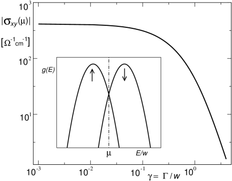
Figure 1: Anomalous Hall conductivity for two band model as a function of the fluctuation strength $\Gamma=\hbar/2\tau$. Inset shows corresponding density of states.

The anomalous Hall conductivity dependence on the fluctuation strength $\Gamma$ shows the same qualitative features as that found for multi-$d$-orbital tight-binding model developed by Kontani et al Kontani_2 . In the case of a weak disorder, $\Gamma/\Delta E_{a}\ll 1$, conductivity is nearly constant while for strong disorder, $\Gamma/\Delta E_{a}>1$, it decreases with a power of the electron life time $\tau=\hbar/\Gamma$, which for the present example even slightly exceeds quadratic dependence. In comparison with the procedure used by Kontani et al whose evaluation is based on the conductivity formula including only velocity operators, presented treatment based on local orbital polarization moments is much simpler and has a clear interpretation. Ferromagnetic state, necessary for appearance of anomalous Hall conductivity, can be characterized by average spin along magnetization axis which is supposed to be parallel with $\hat{z}$ direction. In the case of the considered two-band model it is assumed that each of them is fully spin-polarized but in opposite directions, $s_{z}=\pm 1/2$. If there are no fluctuations the average spin per site $\langle s_{z}\rangle$ reaches a maximum value. Fluctuations of orbital energies can only lead to suppression of this value. The dependence of $\langle s_{z}\rangle$ on the parameter $\Gamma$ representing fluctuation strength is presented in Fig. 2 for the same set of parameters as that used for dependence presented in Fig. 1. It shows the same qualitative features as the dependence of the Hall conductivity on $\Gamma$. In the region where $\langle s_{z}\rangle$ is smaller than its maximum value the Hall conductivity depends on the fluctuation strength. It is the region in which the disorder is strong enough to weaken ferromagnetic state.

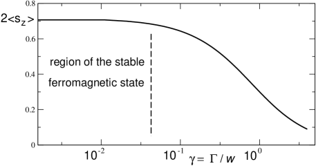
Figure 2: Average spin $\langle s_{z}\rangle$ per site for two band model as a function of the fluctuation strength $\Gamma=\hbar/2\tau$. Model parameters are the same as that used for the dependence presented in Fig. 1.

The simplest approach for diagonal conductivity component $\sigma_{xx}$, Eq. (21), is to neglect vertex corrections, i.e. to use decoupling $\langle GvG\rangle_{\rm av}\rightarrow\langle G\rangle_{\rm av}v\langle G\rangle_{\rm av}$. In this approximation relaxation time coincides with electron life time $\tau=\hbar/2\Gamma$. Using virtual crystal approximation for the considered two-band model and probability distribution of fluctuations, Eq. (21), evaluation of $\sigma_{xx}$ becomes trivial. In Fig. 3 obtained scaling of the Hall conductivity with $\sigma_{xx}$ is shown. It reveals typical features observed experimentally Nagaosa2009 ; Miyasato . Especially the case of the moderate disorder (good metal regime) for which $|\sigma_{xy}|\sim(\sigma_{xx})^{0}$ and that of the strong disorder (bad metal / hopping regime) for which $|\sigma_{xy}|\sim(\sigma_{xx})^{1.6}$.

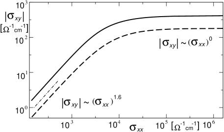
Figure 3: Scaling of the Hall conductivity $\sigma_{xy}$ with longitudinal conductivity $\sigma_{xx}$. Full line is given by the same model parameters as that used for the dependence presented in Fig. 1 while for dashed line the parameters $\kappa$ and $\varepsilon\equiv\Delta E_{a}/w$ have been changed ($\kappa=0.5$ and $\varepsilon=0.4$). Dashed-dotted line shows the slope 1.6.

VII Concluding remarks

Transport theories of conductivity are traditionally formulated to give expressions containing velocity matrix elements only. In the presented treatment the Hall conductivity has been expressed in terms containing also position operator. It has been found that only on-energy-shell matrix elements of both operators are relevant, Eq. (30). For Bloch electron systems the Hall conductivity is given by a part of the orbital magnetization of Fermi electrons, called orbital polarizability momentum, Eqs. (32) and (33), which is a quantity determined by atomic-like orbitals. For a perfect Bloch system it is equivalent to the expression given by the Berry phase curvatures, Eq. (38).

To test applicability of the derived alternative expression for the Hall conductivity, Eq. (30), the two-band model based on the tight-binding approach has been used. Disorder has been modelled by energy fluctuations of single site orbitals. It represents intra-band scattering which can be identified with the so called side-jump scattering. However, this simple model excludes effect of the skew scattering since spin of electrons is supposed to be fixed. Despite of its simplicity it correctly describes scaling of the anomalous Hall conductivity $\sigma_{xy}$ with diagonal conductivity component $\sigma_{xx}$ in the region covering the so called good metal regime, $|\sigma_{xy}|\sim(\sigma_{xx})^{0}$, and the bad metal (hopping) regime, $|\sigma_{xy}|\sim(\sigma_{xx})^{1.6}$. The bad metal regime has been identified with the regime in which disorder becomes strong enough to weaken ferromagnetic state. It remains an open question if the presented form of the general expression for the Hall conductivity in terms of the local orbitals could also be effective in description of the skew scattering effect.

To estimate anomalous Hall conductivity for a real material requires knowledge of local orbitals represented by Wannier functions and also the specific form of fluctuations relevant for the studied system. In particular, finite temperature spin fluctuations are expected to be essential. It is a challenge to work out such a procedure based on the first principle calculations. Newly developed numerical techniques allowing to establish Wannier functions giving the best tight-binding model parameters Marzari ; Wang seem to be a proper way to establish the fluctuation effect upon the anomalous Hall effect in real materials.

Appendix A

Periodic part of Bloch functions can be expressed via Wannier functions $\phi_{n}(\vec{r}-\vec{R}_{l})$ as follows

$$u_{n,\vec{k}}(\vec{r})\,=\,\frac{1}{\sqrt{N}}\sum_{l=1}^{N}e^{i\vec{k}(\vec{R}_{l}-\vec{r})}\phi_{n}(\vec{r}-\vec{R}_{l})\;,$$ (49)

where by definition Wannier functions are orthonormal with respect to their mass-center position vector $\vec{R}_{l}$. The expectation value of the position vector $\vec{r}$ reads

$$\vec{r}_{n}(\vec{k})\,=\,\langle n,\vec{k}|\vec{r}\ n,\vec{k}\rangle\,=\,\qquad\qquad$$

$$=\frac{1}{2}\int\left[u^{+}_{n,\vec{k}}(\vec{r})\,\vec{r}\,u_{n,\vec{k}}(\vec{r})+u_{n,\vec{k}}(\vec{r})\,\vec{r}\,u^{+}_{n,\vec{k}}(\vec{r})\right]dr^{3}=$$

$$=\sum_{l=1}^{N}\int u^{+}_{n,\vec{k}}(\vec{r})\,\frac{\vec{r}-\vec{R}_{l}}{2\sqrt{N}}\,e^{-i\vec{k}(\vec{r}-\vec{R}_{l})}\,\phi_{n}(\vec{r}-\vec{R}_{l})\,d^{3}r+$$

$$+\sum_{l=1}^{N}\int u_{n,\vec{k}}(\vec{r})\,\frac{\vec{r}-\vec{R}_{l}}{2\sqrt{N}}\,e^{i\vec{k}(\vec{r}-\vec{R}_{l})}\,\phi^{+}_{n}(\vec{r}-\vec{R}_{l})\,d^{3}r+$$

$$+\!\sum_{l,l^{\prime}=1}^{N}\frac{\vec{R}_{l}}{2N}\!\int\!\!e^{i\vec{k}(\vec{R}_{l}-\vec{R}_{l^{\prime}})}\phi_{n}^{+}(\vec{r}-\vec{R}_{l^{\prime}})\,\phi_{n}(\vec{r}-\vec{R}_{l})\,d^{3}r+$$

$$+\!\sum_{l,l^{\prime}=1}^{N}\frac{\vec{R}_{l}}{2N}\!\int\!\!e^{i\vec{k}(\vec{R}_{l^{\prime}}-\vec{R}_{l})}\phi_{n}(\vec{r}-\vec{R}_{l^{\prime}})\,\phi_{n}^{+}(\vec{r}-\vec{R}_{l})\,d^{3}r=$$

$$=\frac{i}{2}\int\!\!\left(u^{+}_{n,\vec{k}}(\vec{r})\,\vec{\nabla}_{\vec{k}}u_{n,\vec{k}}(\vec{r})-u_{n,\vec{k}}(\vec{r})\,\vec{\nabla}_{\vec{k}}u^{+}_{n,\vec{k}}(\vec{r})\right)d^{3}r+$$

$$+\frac{1}{N}\sum_{l=1}^{N}\vec{R}_{l}\;,\qquad$$ (50)

where the last constant term represents the center of mass of the considered electron system. For states with $-\vec{k}$ the above relation gives

$$\vec{r}_{n}(-\vec{k})={\rm Im}\int\!\!u^{+}_{n,-\vec{k}}(\vec{r})\,\vec{\nabla}_{\vec{k}}\,u_{n,-\vec{k}}(\vec{r})\,d^{3}r+\frac{1}{N}\sum_{l=1}^{N}\vec{R}_{l}\;.$$ (51)

In the summation over Fermi surface states of the product $\vec{r}_{n}(\vec{k})\,\vec{v}_{n}(\vec{k})$ entering Eq. (33) the mass-center position of the electron system is cancelled out since $\vec{v}_{n}(\vec{k})=-\vec{v}_{n}(-\vec{k})$. The last term on the right-hand side of the above equation can thus be excluded from the consideration since it does not affect the final result.

References

- (1) N. Nagaosa, J. Sinova, S. Onoda, A. H. MacDonald and N. P. Ong, arxiv:0904.4154.
- (2) R. Karplus, and J. M. Luttinger, Phys. Rev. 95, 1154 (1954).
- (3) M. Miyazawa, H. Kontani, and K. Yamada, J. Phys. Soc. Jpn. 68, 1625 (1999).
- (4) M. Onoda and N. Nogaosa, J. Phys. Soc. Jpn. 71, 19 (2002).
- (5) R. Shindou and N Nagaosa, Phys. Rev. Lett. 87, 116801 (2001).
- (6) H. Kontani, T. Tanaka, D. S. Hirashima, K. Yamada, and J. Inoue, Phys. Rev. Lett. 100, 096601 (2008).
- (7) L. Berger, Phys. Rev. B 2, 4559 (1970).
- (8) J. Smit, Physica (Amsterdam) 24, 39 (1958).
- (9) J. M. Luttinger, Phys. Rev. 112, 739 (1958).
- (10) N. A. Sinitsyn, A. H. MacDonald, T. Jungwirth, V. K. Dugaev, and J. Sinova, Phys. Rev. B 75, 045315 (2007).
- (11) E. N. Adams, and E. I. Blount, J. Phys. Chem. Solids 10, 286 (1959).
- (12) R. C. Fivaz, Phys. Rev. 183, 586 (1969).
- (13) P. Středa, T. Jonckheere, arXiv:1002.3212.
- (14) G. Sundaram and Q. Niu, Phys. Rev. B 59, 14915 (1999).
- (15) Yugui Yao, L. Kleinman, A. H. MacDonald, J. Sinova, T. Jungwirth, Ding-sheng Wang, Enge Wang and Q. Niu, Phys. Rev. Lett. 92, 037204 (2004).
- (16) T. Miyasato, N. Abe, T. Fujii, A. Asamitsu, S. Onoda, Y. Onose, N. Nagaosa, and Y. Tokura, Phys. Rev. Lett. 99, 086602 (2007).
- (17) H. Kontani, T. Tanaka, and K. Yamada, Phys. Rev. B 75, 184416 (2007).
- (18) Time dependent potential fluctuations are supposed to be so slowly varying in time that electron states at given time are determined by the eigenvalue problem defined by the static potential just equal to that at given time.
- (19) R. Kubo, J. Phys. Soc. Japan 12, 570 (1957); R. Kubo, A. Yokota, and S. Nakajima, J. Phys. Soc. Japan 12,1203 (1957).
- (20) In the derivation the terms containing the expression of the form have been neglected since they are proportional to infinitesimal after any averaging procedure.
- (21) A. Bastin, C. Lewinner, O. Betbeder-Matibet and P. Nozieres, J. Phys. Chem. Solids 32, 1811 (1971).
- (22) D. A. Greenwood, Proc. Phys. Soc. (London) 71, 585 (1958).
- (23) L. Smrčka and P. Středa, J. Phys. C: Solid State Phys. 10, 2152 (1977).
- (24) P. Středa, J. Phys. C: Solid State Phys. 15, L717 (1982); 15, L1299 (1982).
- (25) A. Crepieux, and P. Bruno, Phys. Rev. B 64, 094434 (2001).
- (26) P. Středa, phys. stat. sol. (b) 125, 849 (1984).
- (27) P. Středa, T. Jonckheere, and T. Martin, Phys. Rev. Lett. 100, 146804 (2008).
- (28) J. Hubbard, Proc. Roy. Soc. (London) A 281, 401 (1964).
- (29) B. Velick y, S. Kirkpatrick, and H. Ehrenreich, Phys. Rev. 175, 747 (1986).
- (30) N. Marzari, and D. Vanderbilt, Phys. Rev. B 56, 12847 (1997).
- (31) X. Wang, J. R. Yates, I. Souza, and D. Vanderbilt, Phys. Rev. B 74, 195118 (2006).