Scalelength of disc galaxies

Abstract

We have derived disk scale lengths for 30374 non-interacting disk galaxies in all five SDSS bands. Virtual Observatory methods and tools were used to define, retrieve, and analyse the images for this unprecedentedly large sample classified as disk/spiral galaxies in the LEDA catalogue. Cross correlation of the SDSS sample with the LEDA catalogue allowed us to investigate the variation of the scale lengths for different types of disk/spiral galaxies. We further investigat asymmetry, concentration, and central velocity dispersion as indicators of morphological type, and are able to assess how the scale length varies with respect to galaxy type. We note however, that the concentration and asymmetry parameters have to be used with caution when investigating type dependence of structural parameters in galaxies. Here, we present the scale length derivation method and numerous tests that we have carried out to investigate the reliability of our results. The average $r$-band disk scale length is $3.79$ kpc, with an RMS dispersion of $2.05$ kpc, and this is a typical value irrespective of passband and galaxy morphology, concentration, and asymmetry. The derived scale lengths presented here are representative for a typical galaxy mass of $10^{10.8\pm 0.54}\rm{~{}M}_{\odot}$, and the RMS dispersion is larger for more massive galaxies. Separating the derived scale lengths for different galaxy masses, the $r$-band scale length is $1.52\pm 0.65$ kpc for galaxies with total stellar mass $10^{9}$–$10^{10}\rm{~{}M}_{\odot}$ and $5.73\pm 1.94$ kpc for galaxies with total stellar mass between $10^{11}$ and $10^{12}\rm{~{}M}_{\odot}$. Distributions and typical trends of scale lengths have also been derived in all the other SDSS bands with linear relations that indicate the relation that connect scale lengths in one passband to another. Such transformations could be used to test the results of forthcoming cosmological simulations of galaxy formation and evolution of the Hubble sequence.

1 Introduction

The exponential scale length of a galaxy disk is one of the most fundamental parameters to determine its morphological structure as well as to model its dynamics, and the fact that the light distributions are exponential makes it possible to constrain the formation mechanisms (Freeman, 1970). The scale length determines how the stars are distributed throughout a disk, and can be used to derive its mass distribution, assuming a specific M/L ratio. Ultimately, this mass distribution is the primary constraint for determining the formation scenario (e.g., Lin & Pringle, 1987; Dutton, 2009, and referenced therein), which dictates the galaxy’s evolution. As the galaxy evolves, substructures such as bulges, pseudo-bulges, bars, rings, and spiral arms may build up, and this will then considerably change the morphology of the host disks (Combes & Elmegreen, 1993; Elmegreen et al., 2005; Bournaud et al., 2007). The scale length value is intimately connected to the circular velocity of the galaxy halo, which in turn relates closely to the angular momentum of the halo in which the disk is formed (Dalcanton et al., 1997; Mo et al., 1998). Up to the last few years, cosmological simulations were limited to rather low resolution, were disks and spheroids were barely resolved, and generally limited to high redshifts, so reproducing realistic disk scale lengths for modern galaxies was clearly out of reach. The current simulations reach resolutions that allow resolving the disks from high redshift down to redshift zero, and subtle mechanisms changing the disk masses and scale lengths can be studied (e.g., Ceverino et al., 2010; Governato et al., 2010; Martig & Bournaud, 2010; Schaye et al., 2010, listed in alphabetic order), thus calling for a comprehensive observational determination of these parameters to test the state of the art cosmological simulations.

Previous observations of NGC, UGC, and low surface brightness galaxies have shown that scale lengths span over a range of three orders of magnitudes (e.g., Boroson, 1981; Romanishin et al., 1983; van der Kruit, 1987; Schombert et al., 1992; Knezek, 1993; de Jong, 1996). Any physical galaxy formation scenario should be able to explain this wide range of values while simultaneously explaining the similarities among disk galaxies throughout this range.

Analytic disk formation scenarios predict that, in cases where angular momentum is conserved, the disk scale length is determined by the angular momentum profile of the initial cloud (Lin & Pringle, 1987), and the scale length in a viscous disk is set by the interplay between star formation and dynamical friction (Silk, 2001). These processes form the basis of a galaxy’s gravitational potential, and determine the strength of gravitational perturbations, the location of resonances in the disk, the formation and evolution of spiral arms and bars, kinematically decoupled components in centres of galaxies, and the dynamical feeding of circumnuclear starbursts and nuclear activity (e.g., Elmegreen et al., 1996; Knapen, 2004; Fathi, 2004; Kormendy & Kennicutt, 2004).

Photometrically, one generally derived this scale length by azimuthally averaging profiles of the surface brightness which is in turn decomposed into a central bulge and an exponential disk, and when spatial resolution allows other components such as one or several bars and rings can be taken into account.

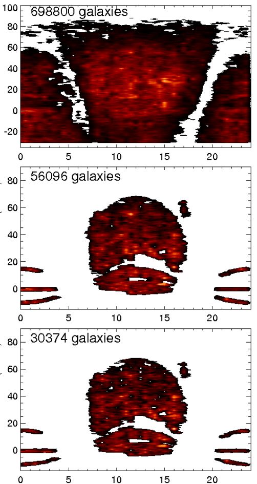
Figure 1: Top: right ascension and declination distribution of the galaxies for which the LEDA services provide a Hubble classification number $\geq 1$ (irrespective of classification error). Middle: same for the 56096 SDSS galaxies fulfilling the first sorting criteria described in section 2.1, and Bottom: the final sample of 30374 selected SDSS disk galaxies for which we have reliable scale $r$-band scale lengths (regardless of uncertainty in the morphological classification, see also section 3.3).

As images in different bands probe different optical depths and/or stellar populations, it is likely that a derived scale length value should depend on waveband, and these effects may vary as a function of galaxy type where different amounts of dust and star formation are expected. Dusty disks are more opaque, resulting in larger scale length values in bluer bands when compared with red and/or infrared images. Similar effects can also be caused by differences in the stellar populations. Differences in scale length as a function of passband can therefore be used to derive information about the stellar structure and contents of galactic disks. Both the effects of stellar populations and dust extinction have been subject to much discussion over the years (e.g., Simien & de Vaucouleurs, 1983; Kent, 1985; Valentijn, 1990; van Driel et al., 1995; Peletier et al., 1994, 1995; Beckman et al., 1996; Courteau, 1996; Cunow, 1998; Baggett et al., 1998; Prieto et al., 2001; Graham, 2001; Graham & de Blok, 2001; Cunow, 2001; Giovanelly & Haynes, 2002; MacArthur, 2003; Cunow, 2004; Graham & Worley, 2008). A detailed and extensive analysis of the dust effects has also been presented for a few tens of galaxies in Holwerda (2005) and subsequent papers by this author, however, as noted by Peletier et al. (1994) and van Driel et al. (1995), the scale length alone in different wavelengths in small sample cannot be used to break the age/metallicity and dust degeneracies. Investigating the scale length variation as a function of inclination for large numbers of galaxies is necessary to distinguish between the effects of dust and stellar populations.

The common denominator in all the previous studies is the roughly comparable sample sizes (at most few hundred galaxies). Most studies have so far analysed individual galaxies, or samples containing a few tens, and in unique cases a few hundred (e.g., Knapen & van der Kruit, 1991; Courteau, 1996), galaxies. Although a number of great results from studies with the Sloan Digital Sky Survey (SDSS; York et al., 2000) in the last years have appeared, these works have not studied the astrophysical parameters targeted here.

As a part of a European Virtual Observatory Astronomical Infrastructure for Data Access (Euro-VO AIDA) research initiative, we have undertaken a comprehensive analysis of the scale length in disk galaxies using an unprecedentedly large sample of disk galaxies. We have used the Virtual Observatory (VO) tools to retrieve data in all ($u$, $g$, $r$, $i$, and $z$) bands from the sixth SDSS major data release (DR6; Adelman-McCarthy et al., 2008) which includes imaging catalogues, spectra, and redshifts freely available. We use the LEDA catalogue (Paturel et al., 2003) to retrieve morphological classification information about our sample galaxies, and those with types defined as Sa or later are hereafter refereed to as disk galaxies (distribution of both samples are presented in Fig. 1).

In the present paper, we present the data retrieval and analysis method used to automatically derive the scale lengths for a sample of disk galaxies which contains 56096 objects (described in section 2), and after rigourous tests described in section 3, we find that a subset of 30374 of these can be called reliable following these criteria. The scale lengths presented here relate only to the disk components, and we have tried to avoid the regions that could be dominated by the bulge component, in order to avoid complications related to the uncertainties of bulge-disk decomposition procedure (as demonstrated in, e.g., Knapen & van der Kruit, 1991). In section 4 we present the first results based on our unprecedentedly large sample of galaxies and finally discuss their implications in section 5.

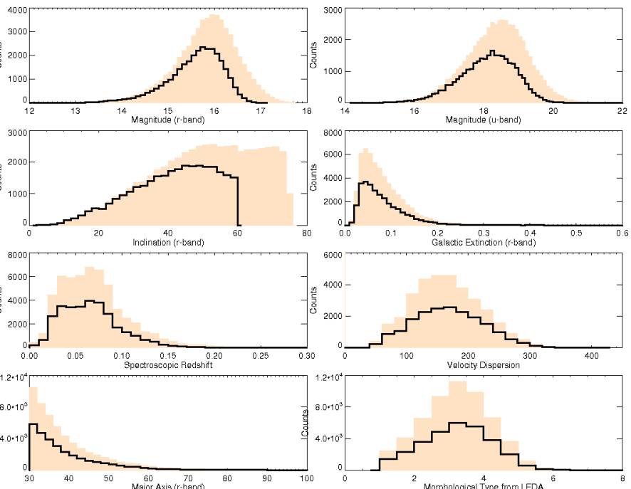
Figure 2: Distribution of some key parameters retrieved from the SDSS database and morphological types from LEDA (bottom right). The filled histograms are the 56096 disk galaxies described in section 2.1, and the open histograms show the distributions of the final 30374 galaxies for which we derive reliable scale lengths. The distribution of the sample remains unchanged.

2 Sample Galaxies from SDSS

2.1 First Selection Criteria

The DR6 provides imaging catalogues, spectra, and redshifts for the third and final data release of SDSS-II, an extension of the original SDSS consisting of three sub projects: The Legacy Survey, the Sloan Extension for Galactic Understanding and Exploration, and a Supernova survey. The SDSS Catalogue Archive Server Jobs System allow for a sample selection based on a number of useful morphological and spectroscopic parameters provided for all objects. We use these parameters and make a first selection of the entire SDSS DR6 sample. Various VO methods were investigated to perform the download of the SDSS images, and the SkyView was chosen for this task. This service has the advantage of being able to create fits cut outs centred at a given sky coordinate and with a given size. Moreover, SkyView is able to re-scale the image backgrounds to the same level, hence correcting for background level differences between the SDSS tiles.

The image size is an important parameter to achieve a reliable sky subtraction which is necessary to derive realistic scale lengths, thus we require that the images cover an area at least three times the size of each galaxy. To optimise the data handling and keep low data transfer time from SkyView, we chose a constant image size of $900\times 900$ pixels to be sampled for all galaxies, still being able to achieve a reliable sky subtraction. With these specifications, the image size is 3.2 MB with the typical download time of 16 seconds per image. This also includes the time that SkyView spends cutting, mosaicing, and re-scaling images.

Our first selection criteria uses SDSS parameters to ensure that:

1)

The object is a galaxy, and has good quality images available, i.e., quality keyword $\geq 2$.

2)

The galaxy is at a position with low $r$-band Galactic extinction $A_{r}\leq 1.0$. In reality, we find that 99% of the sample have $A_{r}\leq 0.25$.

3)

For each galaxy SDSS provides spectroscopic redshift measurement, i.e., galaxy $r$-band magnitude $\leq 17.7$.

4)

The galaxy diameter is at least 60 pixels ($=24\arcsec$) and at most 200 pixels ($=80\arcsec$ in diameter). The first criterion ensures that the derived light profile samples the disk with at least 10 data points (for two-pixel wide rings) to derive the scale length, and the second criterion is for an optimised data retrieval procedure described above. Here we use the $r$-band isophotal semi major-axis $isoA$ and semi minor-axis $isoB$ as a measure for the galaxy size.

5)

High inclination ($incl.\geq 70$ degrees) galaxies are removed to avoid selection effect problems, but also since scale lengths for such systems are not reliable. The inclination is determined using the ratio between the semi minor axis $isoB$ and semi major axis $isoA$ in the $r$-band from the SDSS parameter list ($\cos i=isoB/isoA$).

5)

No redshift cut was applied, however, Fig. 2 shows that the sample extends out to redshift 0.3, with the typical redshift at $\log z=-1.2$ derived with $\geq 0.995$ confidence level, and with $15\%$ of the sample with $\log z\geq-1.0$.

This first set of criteria leaves us with a total of 95735 galaxies. We use the LEDA services to retrieve a numeric Hubble classification parameter $T$ for the galaxies in our sample (more on this in section 4.1). We first download the entire LEDA catalogue, which we cross-correlate with the SDSS sample using TOPCAT and only select the galaxies which, in LEDA, are classified as spiral galaxies (i.e., $1\leq T\leq 8$). A total of 56096 Sa-Sd (i.e., $T$ between 1 and 8) spiral galaxies (see Fig. 1) were found, for which SDSS $u,g,r,i,z$-band images were downloaded. In section 4.1, we further discuss whether all these galaxies are well-classified disk or spiral galaxies.

In Fig. 2, we show the distribution of some key parameters retrieved from the SDSS and LEDA database. This figure shows that the different sample selection stages do not introduce any biases in our sample. It should be noted that, at this stage, we are unable to determine whether the galaxies in our sample are isolated or disturbed systems, as this information is not provided by any of the catalogues we have used. We make this distinction using the asymmetry parameter described in Schade et al. (1995).

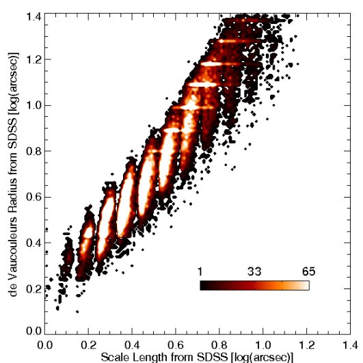
Figure 3: Density plot of the de Vaucouleurs effective radius ($y$-axis) versus exponential disk radius ($x$-axis) provided by the SDSS service for the entire disk galaxy sample. The odd clustering of the data (overdensities around discrete values) show the strong systematic effects in these two parameters provided by the SDSS team.

2.2 Scale lengths from SDSS

The first issue that arises at this point is the fact that SDSS services provides users with the disk scale length as well as de Vaucouleurs effective radius for each galaxy (in all bands), and that, in principle, these values could be used to carry out our analysis. In Fig. 3, we show that the values provided by the SDSS services show anomalies that are beyond our satisfaction for carrying out our analysis. The plot shows peculiar systematic effects in their derivation of the de Vaucouleurs radii and scale lengths around some discrete values marked by the overdensities, the source and explanations for which we cannot find. We thus decide to re-calculate the scale lengths.

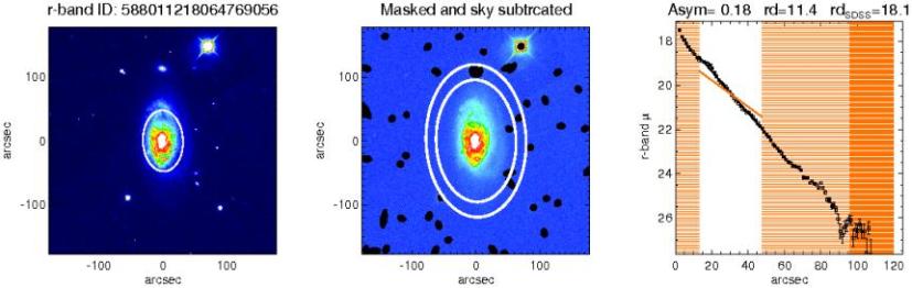
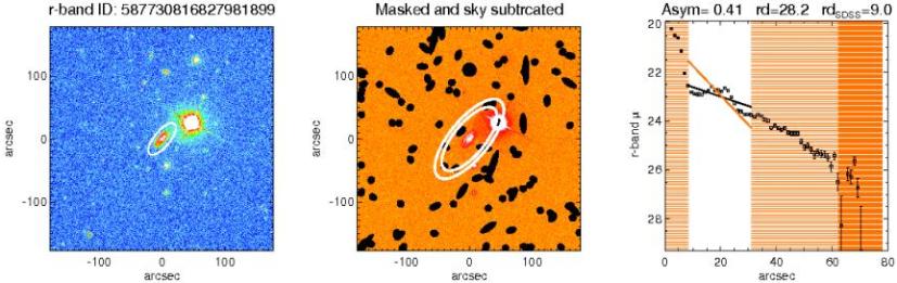
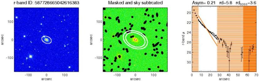
Figure 4: Three randomly selected galaxies for which we illustrate the procedure for deriving the scale length (see section 3). For each galaxy, the left panel shows the $r-band$ image and the ellipse with axis-ratio $isoB/isoA$. The middle panel shows the sky-subtracted image, the sky region $2.0\pm 0.25\times isoA$ outlined by two corresponding ellipses, and the SExtractor sources masked. The right panel shows the light profile using the zero point from the SDSS, and linear fit to the disk region as described in section 3. At the top this panel, the asymmetry parameter, our derived disk scale length (black linear fit) and the scale length from SDSS (arbitrarily shifted red line) are stated.

3 Deriving Scale lengths and Asymmetries

3.1 Using IDL and GDL

To derive the disk scale length, we use some important parameters provided by the SDSS in order to constrain galaxy geometry as well as the location of the sky region. These are semi minor axis $isoB$, semi major axis $isoA$, isophotal position angle $isoPhi$, and for consistency, we use these $r$-band quantities in also in all other bands. Our scale length derivation routine uses standard IDL routines, though due to license limitations this code can only be executed once, and hence is estimated to take a long time to run. Using one single IDL session, we would need 47 days to derive the scale lengths for the entire sample, thus in order to speed up the process, we decided to run this computation on a cluster of machines located at Centre de Données astronomiques de Strasbourg CDS. Since the freely available IDL virtual machine does not allow one to launch batch queries, and since installing an IDL licence on each cluster node was not an option, we used the open source clone of IDL, GNU Data Language GDL (Coulais et al., 2009). We found out that a few IDL functions were either missing or behaving improperly, thus requiring minor tweaking in our code. Then, we ran both IDL and GDL code on the same subset of SDSS images, in order to check the reliability of the GDL output.

Once the GDL code was installed on each node of the cluster, the 56096 SDSS images were put to an iRods installation deployed at CDS. Finally, the scale length computation was launched on the cluster, using the following architecture:

1. A Java program holds the list of galaxies to process, and - for each object of this list - sends a message to the cluster, asking to spawn a new job (i.e., launch the corresponding computation).

2. The cluster master node receives the request, and dispatches it to the cluster node with the smallest CPU load.

3. The cluster node then downloads from iRods the $u,g,r,i,z$ images corresponding to the galaxy to process, runs the GDL code, and sends back the computed result to iRods.

4. If the computation fails, it will be re-sent to another node until success

The CDS cluster has proven to be very stable and reliable, though some problems were found in the dispatching algorithm, resulting sometimes in overloading some of the nodes while some others were idle. Four nodes of the cluster were dedicated to our computation. As the total computation time is roughly proportional to the number of involved nodes, allocating ten times more nodes would have decreased this time by a factor ten. This would only be true if the computation service were to be close to the data, so that the transfer time would be negligible with respect to the computation time. In theory, on the CDS cluster, with four dedicated nodes, we should have been able to process 11200 galaxies per day, however in reality, the cluster only processed between 8500 and 9000 galaxies per day, which could be explained by some inefficiency in the dispatching algorithm. To conclude, using the CDS, we have been able to derive the scale lengths for all 56090 galaxies in all five SDSS bands in less than a week.

3.2 The Procedure

The procedure to derive scale length and calculate asymmetry parameters from the SDSS images is illustrated in Fig. 4 and carries out the following steps:

• Reading the image and assigning the pre-determined $r$-band parameters from a file that contains all SDSS parameters for the entire sample.

• Selecting the sky region as the ellipse encompassing the range $2.0\pm 0.25\times isoA$. This is marked as a darker shaded region in the rightmost panels in Fig. 4. The mean value of this region, using Tukey’s bi-weight mean formalism described in Mosteller & Tukey (1977), is used to calculate the sky level for sky subtraction as well as setting the background level.

• To remove foreground stars and point sources from the image, we extract point sources with SExtractor (Bertin & Arnouts, 1996), by selecting all point sources that are larger than 4 pixels in size and more than 3 $\sigma$ above the background level. All pixels belonging to these sources are then masked out, and we note that our selection could include bright star-forming regions and small background galaxies in these sources.

• Using the asymmetry parameter definition of Schade et al. (1995) and Conselice (2003), we calculate the asymmetry parameter

  $$A=\sum\|I-I_{180}\|/\sum I,$$ (1)

  where $I$ is the sky subtracted galaxy image intensity and $I_{180}$ is that for the image rotated by 180 degrees around the galaxy centre. It should be noted here that the asymmetry criterion applied here removes ongoing mergers and galaxies with companions at a projected distance of about twice the galaxy radius, and here we take the results of Conselice (2003) at face value, that $A\geq 0.35$ means that the system is disturbed.

• Using the $isoB$, $isoA$, $isoPhi$ parameters from SDSS, we then section each galaxy into 2-pixels wide ellipses oriented at the major axis position angle $isoPhi$ and with minor-to-major axis ratio $b/a=isoB/isoA$. The bi-weighted mean surface brightness value within each ellipse is calculated to compile the galactocentric surface brightness profile $\mu(r)$ for each galaxy.

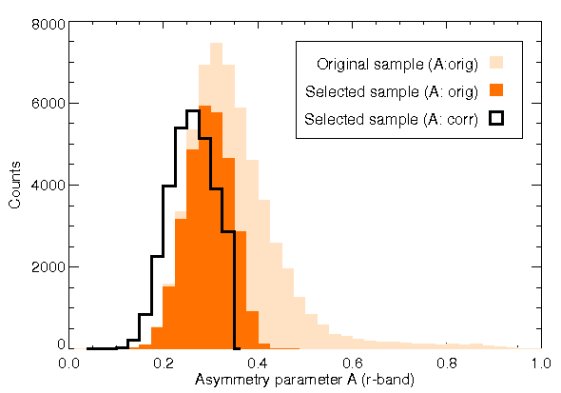
Figure 5: Asymmetry parameter for all 56096 disk galaxies assuming the objects are located in the centre of the image (grey histogram), and when the galaxy image is rotated around the “true” galaxy centre found by centroid fitting (red histogram). The final set of 30374 low-inclination and low-asymmetry galaxies for which we derive the scale lengths are shown with the black histogram.

In spatially resolved systems, surface brightness profiles are commonly fitted by a multiple of parametric functions in order to describe the contribution of different components to the observed profile. A de Vaucouleurs ($r^{1/4}$, de Vaucouleurs, 1948) or Sérsic ($r^{1/n}$, Sérsic, 1968) law is typically used for the innermost part of the disk, and for the outer parts an exponential function of the form

$$\mu(r)=\mu_{0}+1.086\,\frac{r}{r_{d}},$$ (2)

is used, where $\mu_{0}$ is the central surface brightness, $r$ is the galactocentric radius, and $r_{d}$ is the disk scale length of the outer disk. In addition to these two components, other functions may be used to fit the halo component, bars, rings, and other structures in the galaxies (e.g., Prieto et al., 2001), and the fits can be applied to one-dimensional light profiles or directly on two-dimensional images (Byun & Freeman, 1995). Here we fit equation (2) to the one-dimensional surface brightness profiles.

Running the fully automated fitting algorithm on all retrieved images, we found a number of artefacts which cause problems for applying the code successfully. These include:

• SkyView does not deliver the image for the galaxy in all bands, i.e., a blank image has been transferred and stored. The first query delivered 892 blank images, and a second query on the blank images delivered successfully less than 1% of the images.

• The galaxy is positioned such that there are no adjacent tiles observed yet, and thus a large part of the retrieved image is filled by SkyView with blank pixels.

• The galaxy is too faint in a given band to deliver reliable surface brightness profile, i.e., the linear fit results in a negative slope.

• Man-made satellites passing too close to the galaxy position.

3.3 Reliable Scale Lengths

Saturated stars near the objects cannot be masked properly using SExtractor (due to undetermined source radii). Moreover, strong galaxy interactions and noisy images introduce errors in the derived scale lengths. We selected randomly a few hundred images for which we plot the surface brightness profiles with corresponding linear fits. Visual inspection showed that the routine runs as expected. Saturated stars, if far away from a galaxy (further then $2.25\times isoA$, i.e., the outermost sky pixel) do not introduce any errors in the derived parameters as they are not considered at any stage. If close to a galaxy, they can be regarded as interactions. Interactions between galaxies can be quantified following Conselice (2003) and Conselice et al. (2003) who found that interacting or merging galaxies mostly have asymmetry parameter $A\geq 0.35$.

When applying equation (1), it is crucial to rotate the images around the centre of the galaxy, as minor offsets can significantly overestimate $A$. We apply a centroid fitting to our sample, and find that the images generated by SkyView are off-centred by about half a pixel. This offset, although minor in terms of pixels and arcseconds, significantly over-estimates $A$ for our galaxies (see Fig. 5).

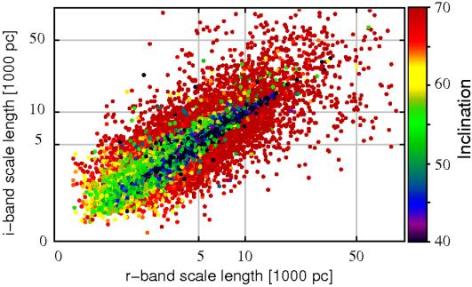
Figure 6: Scale lengths form the $i$-band images ($y$-axis) versus those from $r$-band images ($x$-axis), where the inclination of the galaxy is shown by the colour bar on the right of the figure. Although the points fall on a 1:1 slope, the galaxies with $incl.<60$ degrees have smaller scatter ($\mathfrak{R^{2}}>0.90$, see text in section 3.3).

If the galaxy image is deep enough, it is expected that the scale length values in two adjacent bands should be similar. As images in all SDSS bands are not equally deep, we investigate the $r$ and $i$-band images for this purpose only, since these two filters are comparable, and sufficiently adjacent to deliver almost identical scale lengths. Plotting the corresponding scale lengths, shown in Fig. 6, we find that galaxies with high inclination $incl.\geq 60$ degrees) are the objects that introduce the large scatter in this diagram.

We use Pearson’s product moment correlation coefficient to calculate the coefficient of determination $\mathfrak{R^{2}}$ according to the standard formula

$$\mathfrak{R^{2}}=1-\frac{\displaystyle\sum^{N}_{j=1}(X_{j}-\hat{X}_{j})^{2}}{\displaystyle\sum^{N}_{j=1}(X_{j}-\overline{X})^{2}},$$

where $N$ is the number of data points, $X_{j}$ are the measured data, $\hat{X}_{j}$ are the estimated values given by linear regression, and $\overline{X}$ is the mean value of the measured data points. In simple statistical terms, the numerator is termed the total sum of squares, and the denominator is the error sum of squares, and the coefficient $\mathfrak{R^{2}}$ provides the percent of the variation that can be explained by the linear regression equation, and therefore is a useful measure for the variance of one variable that is predictable from the other variable. If the regression line passes exactly through 50% of the data points, it would be able to explain half of the variation of the linear fit, and would result in $\mathfrak{R^{2}}$=0.5. Throughout our analysis, we trust a correlation if $\mathfrak{R^{2}}\geq 0.9$, and $\mathfrak{R^{2}}\leq 0.68$ is considered insignificant (c.f., less than one-sigma confidence level is insignificant).

The dispersion of the data points around the 1:1 line can is then measured by calculating $\mathfrak{R^{2}}$ for different inclination bins, and we find that this parameter remains above 0.90 for $incl.\leq 60$, hence keep all the galaxies with $incl.\leq 60$ degrees. We will later find that combining the inclination and asymmetry restriction will deliver even higher coefficient of determination between the scale lengths in different bands.

Finally, we find that for five galaxies, the SDSS spectroscopic redshifts are larger than 1, whereas the rest of the sample has redshift $<0.3$. Despite the small redshift errors, we find the redshifts for these five galaxies unrealistic and we choose to remove them from our sample.

Thus, applying these cuts, we derive scale lengths for 30374 disk galaxies that we argue are reliable, given the arguments mentioned above.

Table 1: Disk scale length and central surface brightness for different assumed disk range as a fraction of $isoA$ as illustrated in Fig. 7. The values presented here have been derived for a random sub sample of 800 galaxies with formal errors given in brackets, and all values are normalised to the scale length derived in the range 25%–100%.

Fitted $isoA$ Range	($r$-band) $r_{d}\over r_{d}(25\%-100\%)$	($r$-band) $\mu_{0}\over\mu_{0}(25\%-100\%)$	($i$-band) $r_{d}\over r_{d}(25\%-100\%)$	($i$-band) $\mu_{0}\over\mu_{0}(25\%-100\%)$
0%–100%	0.91(0.19)	0.87(0.18)	1.07(0.12)	1.09(0.12)
20%–100%	0.98(0.08)	0.97(0.07)	1.02(0.05)	1.03(0.05)
25%–100%	1	1	1	1
30%–100%	1.07(0.15)	1.09(0.18)	0.97(0.07)	0.96(0.08)
30%–100%	1.14(0.27)	1.12(0.17)	0.93(0.12)	0.93(0.09)
40%–120%	1.20(0.28)	1.25(0.29)	0.87(0.16)	0.87(0.16)

Table 2: Disk scale length and central surface brightness for different assumed sky range as a fraction of $isoA$ as illustrated in Fig. 8. The values presented here have been derived for a random sub sample of 800 galaxies, normalised to the sky range $2.00\pm 0.25$, with formal errors given in brackets.

Fitted Sky Range	($r$-band) $r_{d}\over r_{d}(2.0\pm 0.25)$	($r$-band) $\mu_{0}\over\mu_{0}(2.0\pm 0.25)$	($i$-band) $r_{d}\over r_{d}(2.0\pm 0.25)$	($i$-band) $\mu_{0}\over\mu_{0}(2.0\pm 0.25)$
$1.75\pm 0.25$	0.99(0.03)	0.99(0.03)	1.00(0.01)	1.00(0.01)
$2.00\pm 0.25$	1	1	1	1
$2.25\pm 0.25$	1.00(0.03)	1.01(0.04)	1.00(0.01)	1.00(0.02)
$2.50\pm 0.25$	1.01(0.05)	1.01(0.07)	1.00(0.02)	1.00(0.03)
$2.75\pm 0.25$	1.01(0.06)	1.01(0.09)	1.00(0.03)	1.00(0.04)

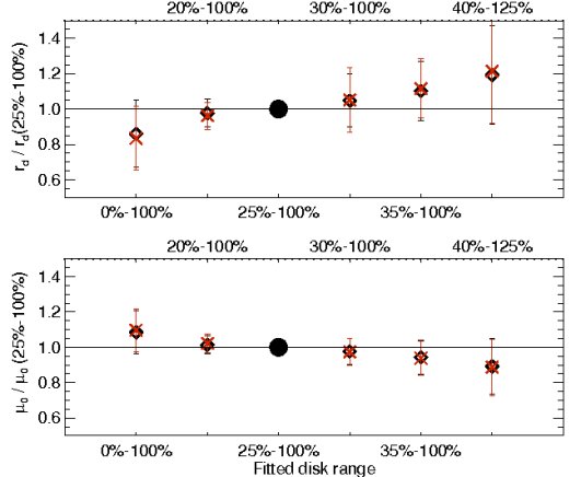
Figure 7: Disk scale length and central surface brightness for different assumed disk range as a fraction of $isoA$ parameter provided by the SDSS. The values illustrated here have been derived for a random sub sample of 800 galaxies in $r$-band (black diamonds) and $i$-band (red crosses). All values have been normalised to that illustrated by the black circle, which is the disk range we assume throughout this work.

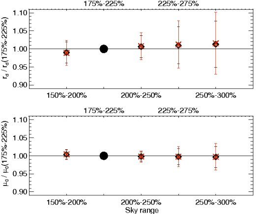
Figure 8: Disk scale length and central surface brightness for different assumed sky range as a fraction of $isoA$ parameter provided by the SDSS. The values illustrated here have been derived for a random sub sample of 800 galaxies in $r$-band (black diamonds) and $i$-band (red crosses). The values have been normalised to that illustrated by the black circle, which is the sky range we assume throughout this work.

3.4 Disk and Sky Ranges

Here, we will not delve into the intricacies of fitting the light curves, but focus on the determination of the scale length of the exponential disk. Despite the long tradition (see references in section 1), the important and comprehensive study by Knapen & van der Kruit (1991) showed that the errors in these data are still significantly large ($\approx 25\%$), especially if they were obtained from photographic plates. The uncertainties depend on image depth, image sky coverage, data reduction, disk region fitting, the order in which bulges, bars, or other components are fitted. These matters become more complicated when analysing with SDSS images which are relatively shallow, and even more so when automatically fitting thousands of galaxies which cover a wide range of brightness and morphologies. To avoid complications that are not related to the nature of our analysis (e.g., Fathi & Peletier, 2003), we have decided to derive the disk scale length simply by fitting an exponential profile to a pre-defined disk region of each galaxy, i.e., the region where we assume the light to be dominated by the exponential profile. This means that we are simply cutting out the central regions of the galaxies where bulges and strong bars are expected.

We determine the disk region by empirically fitting the equation (2) to a set of ranges where we expect the disk to dominate the derived surface brightness profiles. We use the $isoA$ parameter to estimate this range, and randomly select 800 galaxies, to which we apply this test both in $r$ and $i$-band. In Fig. 7, we show the resulting disk scale lengths when fitting the regions presented in Table 2 , and when normalised to our nominal 25%–100% of the $isoA$ radius, we find that the derived scale lengths change by less than 10% for a wide range of assumed disk ranges (seen as the unshaded region in the rightmost panels in Fig. 4). We further note that the distribution of the data points for each test, normalised to the 25%–100% $isoA$ range, is well represented by a Gaussian, and the error bars in Fig. 7 are indeed symmetric.

For a similar test, we assume sky regions at different distances from each galaxy centre and assess the effect of the sky subtraction on the derived scale lengths. Applied to the same randomly selected 800 galaxies, we found that, assuming that the sky is represented by the $2.0\pm 0.25\times isoA$ region, robust scale length and surface brightness measurements are delivered.

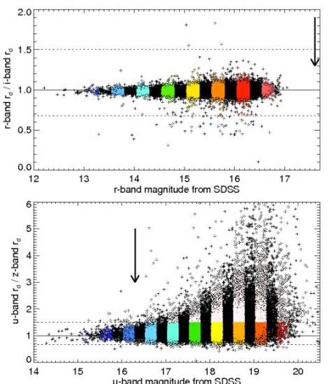
Figure 9: Scale length ratio versus magnitude for two pairs from table 3. Bins of 0.2 magnitude are used to scan the data points ”from left to right”, and when less than 95% of the ratios are inside the dotted lines, that magnitude limit is taken to be the faintest magnitude where we trust the scale lengths for these two bands. Here we show the best case $r,i$-pair (top) and the worst case $u,z$-pair (bottom). In each panel, the arrow indicates the cutting limit presented in table 3.

Table 3: Magnitude cuts applied to the final sample of 30374 galaxies as described in section 3. To apply the cut to each pair, a plot similar to Fig. 9 was set up, and the magnitude cut was decided accordingly.

Filter Pair	Upper Magnitudes	Number of Galaxies
$g$ and $r$	$g<17.70$   &   $r<17.70$	30201
$g$ and $i$	$g<19.95$   &   $i<16.65$	30371
$g$ and $z$	$g<17.70$   &   $z<15.53$	27319
$r$ and $i$	$r<17.70$   &   $i<16.65$	30374
$r$ and $z$	$r<17.70$   &   $z<15.53$	27329
$i$ and $z$	$i<15.89$   &   $z<15.53$	27264
$u$ and $g$	$u<16.79$   &   $g<14.94$	847
$u$ and $r$	$u<16.54$   &   $r<13.56$	132
$u$ and $i$	$u<16.79$   &   $i<13.14$	123
$u$ and $z$	$u<16.29$   &   $z<12.78$	88

3.5 Scale Lengths in $u,g,r,i,z$-bands

Although the SDSS is one of the most influential and ambitious astronomical surveys, the depth of its images in all bands are not equal. Here we have chosen to analyse only the galaxies for which SDSS provides spectroscopic redshifts (in order to investigate the redshift evolution the parameters we derived), where SDSS is complete for $r$-band magnitude $<17.7$. The images in other bands are not equally deep and/or complete to this magnitude limit, partly due to the significantly different transmission curves for the different filters. Including atmospheric extinction and detector efficiency, the peak quantum efficiency of the system in $u$ and $z$-bands are $\approx 10\%$, $g$ and $i$-band $\approx 35\%$, and $r$-band $\approx 50\%$. Thus it is necessary to apply a magnitude cut which varies depending on the band, fainter than which we are not able to derive reliable scale lengths.

For each pair of SDSS filters, we expect that the scale length variation larger than a factor 1.5 is unphysical. We determine the magnitude limit for a pair of filters by plotting the scale length ratio versus magnitude in one of the bands (see Fig. 9), and scan the values from the brighter to the fainter levels in fixed bins of 0.2 magnitudes. Once we reach a magnitude where less than 95% of the scale length ratios is smaller than 0.67 or larger than 1.5 (i.e., above or below the horizontal dotted lines in Fig. 9), we stop the scan and select this value for the faintest magnitude level in that band for which we trust the scale lengths. As shown in Fig. 9, this procedure very clearly demonstrates the noise in different bands, and how the values presented in table 3 have been established. In the given examples, the scale lengths in $r$-band when compared to $i$-band are complete to an $r$-band magnitude of 17.70 (indicated by the arrow), and the $u$ versus $z$-band is complete to an $u$-band magnitude of 16.29 (indicated by the arrow).

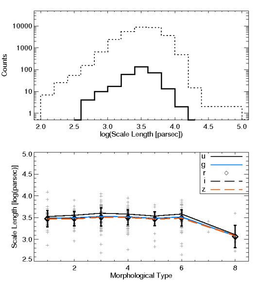
Figure 10: Top: Distribution of the reliably derived $r$-band scale lengths for the entire sample of 30374 galaxies (dotted histogram) and the 309 morphologically well-classified galaxies (solid histogram). Bottom: Scale length versus morphological type for the 309 galaxies which have been morphologically classified accurately. The $r$-band has been used with the scale length in $u,g,i,z$ bands i plotted in the middle panel. The error bars for all bands are comparable, and here we only show these for the $r$-band values.

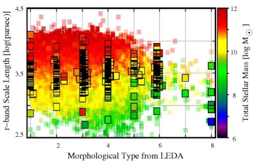
Figure 11: Scale length versus morphological type for the entire sample of 30374 galaxies, with the 309 well-classified galaxies marked with black squares. The colour represents the total stellar mass for each galaxy.

4 Results

4.1 Scale Length versus Morphology

The morphological classification scheme of Sandage (1961), is designed based on visual inspection of basic features of galaxies which relates them to their formation and evolution histories. While this classification scheme is somewhat subjective, in the past years, numerous efforts have been made to define quantitative versions of this classification scheme (e.g., Burda & Feitzinger, 1992; Doi et al., 1993; Abraham et al., 1996; Yamauchi et al., 2005).

The numeric morphological types presented in the LEDA catalogue are a compilation of the morphological types encoded in the de Vaucouleurs scale as well as the luminosity class (van den Bergh’s definition). There is also information about the presence of bars and rings, but we do not consider these for the present paper mostly since this information is only available for minor fraction of the sample. More details about the classification of galaxies can be found in the Level 5 of the NASA/IPAC Extra-galactic Database (NED). The morphological types of LEDA have been compiled using from Vorontsov-Velyaminov et al. (1963); Nilson (1973); Lauberts (1982); de Vaucouleurs et al. (1991); and Loveday (1996).

We select only the galaxies which are classified using the numeric type = 1 (i.e., Sa) up to and including numeric type = 8 (i.e., Sdm). Most of the values presented in Fig. 2 are subject to errors larger than 1, typically smaller for fainter galaxies, but they seem not to depend much on other parameters such as asymmetry, redshift, etc. To analyse the dependency of the parameters with respect to morphological type, we strictly only use the galaxies for which the morphological type error is smaller than 0.5. These are 309 galaxies from our final sample of 30374 galaxies, for which we investigate how the scale length and asymmetry parameter depends on morphology.

Typically, scale lengths for disk galaxies are not expected to depend on Hubble morphological type (de Jong (1996); Graham & de Blok (2001)) for types ranging between 1 and 6. Here, we analyse our derived values in this context first by only using the galaxies for which we only find morphological classifications with corresponding errors smaller than 0.5, i.e., the 309 galaxies explained in section 4.1. In Fig. 10, we plot the $r$-band scale length and morphological types, and find that our sample is fully consistent with previous results showing that the absolute value of the scale length is independent of type. We transform the scale length to parsec units by using the spectroscopic redshifts provided by the SDSS and ignore local flows. Our scale length values agree with those derived by previous authors (e.g., van der Kruit, 1987; Cunow, 2001; de Jong, 1996); we find that the average $r-band$ scale length for the entire sample is $3.79\pm 2.05$ kpc, and that for the 309 galaxies with reliable morphology is $3.3\pm 1.6$ kpc (see top panel of Fig. 10). Further discussion is provided in section 4.2, and the errors are root mean square (RMS) values.

In combination with the mass determination described in section 4.3, we find that the mass does play a certain role in the behaviour of Fig. 10. Although out to type $T=6$ scale length are constant, the later type galaxies ($T>6$) are generally those of lower mass, and hence in agreement with Fig. 15. These lower mass galaxies have smaller scale lengths, thus the scale length decrease for late types is intimately linked with the lower left corner of Fig. 15. However, it should be noted that here we only have used the galaxies with robust morphological classification, and have a smaller number of low-mass galaxies as compared with high-mass galaxies (9 galaxies with total stellar mass $10^{8}-10^{9}\rm{~{}M}_{\odot}$, 40 galaxies with total stellar mass $10^{9}-10^{10}\rm{~{}M}_{\odot}$, and 207 galaxies with total stellar mass $10^{10}-10^{11}\rm{~{}M}_{\odot}$).

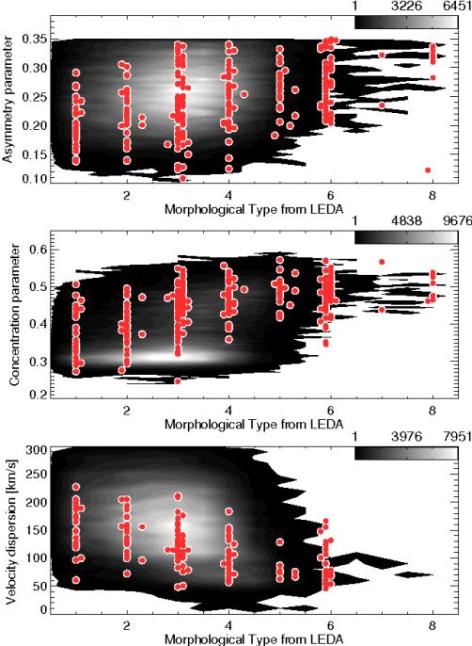
Figure 12: Asymmetry, concentration, and velocity dispersion as type indicator for the full sample (grey density plot) and for accurately (type error $\leq 0.5$) classified galaxies in LEDA.

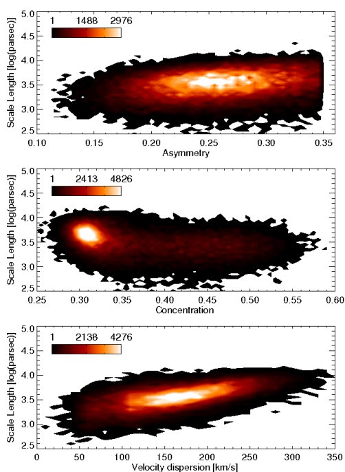
Figure 13: Scale length versus asymmetry and concentration parameter and stellar velocity dispersion for the full sample of 30374 galaxies.

We now cross-correlate our sample with the morphologically classified bright galaxy catalogue of Fukugita et al. (2007). Their catalogue contains 2275 galaxies classified by visual inspection of SDSS images in the $g$-band. We find 283 objects overlapping between the two samples. The small overlap is partly due to the fact that around half of the objects in Fukugita et al. (2007) are early-type galaxies (RC3 type $T<1$), and partly since it is essentially the overlap between the LEDA sample and that of Fukugita et al. (2007). Moreover, our sample has an upper limit for the galaxy sizes due to our preferred strategy for using SkyView (see section 2.1). From this sample of 283 galaxies, only 45 galaxies have been accurately classified (their T error $\leq 1$) in Fukugita et al. (2007). For these objects, we find weak correlation between the morphological classification from LEDA and those from Fukugita et al. (2007).

In a similar fashion to Shimasaku et al. (2001), we define the ”inverse” concentration parameter as the ratio between the radii containing 50% and 90% of the Petrosian flux respectively, $r_{50}/r_{90}$ provided by the SDSS services. As a consistency check, we ensure that we reproduce Fig. 10 of Shimasaku et al. (2001), i.e., that morphological classification provided by LEDA correlates with concentration parameter. Furthermore, we find that although the vast majority of our sample have very large morphological classification uncertainties (T error $\geq 1$), the concentration parameters that we calculate for all 30374 galaxies indicate that, in agreement with Shimasaku et al. (2001), they are disk galaxies.

Regarding the correlation of the concentration parameter with morphological type, for the 309 well-classified galaxies $\mathfrak{R^{2}}=0.31$, and for the full sample $\mathfrak{R^{2}}=0.16$. Although we find these values unconvincing as firm correlations, we acknowledge a clear trend that concentration parameter is increasing with galaxy morphological type. Likewise, the spread of points in asymmetry-type and velocity dispersion-type diagrams are very large, and the coefficients of determination even lower than that of the concentration parameter, however, here also the trend is acknowledged.

Given that robust morphological classification is known only for a very small subset of our entire sample, we invoke other parameters in order to be able to further investigate the scale lengths for the full sample. Following the above arguments, and their consistency with the previous findings by, e.g., Conselice (1997); Shimasaku et al. (2001), and Fukugita et al. (2007) we find it instructive to invoke these parameters as type indicators (see Fig. 12). For example, we find that the asymmetry parameter correlates with type $T$ as $A=0.19+0.02T$, put this into the graph, however, the $\mathfrak{R^{2}}$ varies between 0.05–0.81 depending on bin and choice of sub sample and parameter, with the best correlation for unjustified binning applied. For this reason, we do not quote the errors or mathematical formulation for how $A$, $C$, or velocity dispersion, vary with type, but take these trends as a indications and further investigate how scale length depends on these parameters as morphological type indicators.

In Fig. 13, we plot the scale lengths versus asymmetry, concentration, and velocity dispersion. Although it is shown that scale length decreases at higher concentration parameter, a line-fitting exercise reveals $\mathfrak{R^{2}}=0.12$, which implies insignificant correlation. The velocity dispersion has a higher correlation, $\mathfrak{R^{2}}=0.37$, but still with no strong statistical significance. Moreover, the large scatter of the scale length values illustrated in Fig. 13 is consistent with the galaxies studied by de Jong (1996).

This exercise tells us, firstly, that asymmetry, concentration, and velocity dispersion only correlate weakly with morphological type, and secondly, that even when using these parameters as morphological type indicators, there is no strong change in disk scale length for different galaxy types. Furthermore, we have now been able to use the full sample of 30374 galaxies with reliable scale lengths.

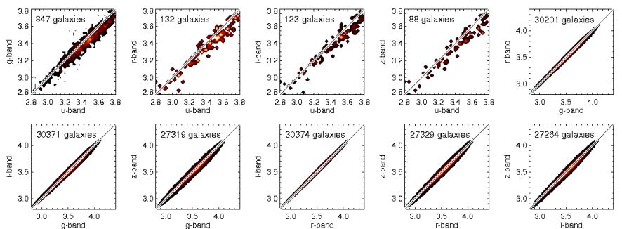
Figure 14: Scale lengths in $u,g,r,i,z$ bands given in decimal logarithm of parsecs, with the number of points in each density plot stated, and the 1:1 line drawn on each panel.

4.2 $u,g,r,i,z$ Scale Lengths

The derived scale lengths can be compared between the images in different bands to investigate the effects of dust and stellar populations in disk galaxies (e.g., Cunow, 2001). Such analysis is complementary to the results on colour gradients used to analyse age gradients in disks (e.g., Cunow, 2004, and many more).

We analyse the derived scale lengths in different bands applying the limits presented in table 3. We can then compare for a given subset, where reliable scale lengths have been derived in two bands, how the scale length changes between different SDSS bands. We derive a series of correlations between the scale lengths in different bands, and although not all band-pair samples are of equal size, we find that the correlations for all the pairs are significant (see equations (3)–(12), where all formal errors and coefficients of determination are given).

$$\log(r_{d}^{g})=0.25(\pm 0.03)+0.91(\pm 0.01)\log(r_{d}^{u})\ \ \mathfrak{R^{2}}=0.94$$ (3)

$$\log(r_{d}^{r})=0.36(\pm 0.08)+0.88(\pm 0.02)\log(r_{d}^{u})\ \ \mathfrak{R^{2}}=0.92$$ (4)

$$\log(r_{d}^{i})=0.32(\pm 0.07)+0.89(\pm 0.02)\log(r_{d}^{u})\ \ \mathfrak{R^{2}}=0.94$$ (5)

$$\log(r_{d}^{z})=0.36(\pm 0.09)+0.88(\pm 0.03)\log(r_{d}^{u})\ \ \mathfrak{R^{2}}=0.92$$ (6)

$$\log(r_{d}^{r})=0.06(\pm 0.01)+0.98(\pm 0.01)\log(r_{d}^{g})\ \ \mathfrak{R^{2}}=0.98$$ (7)

$$\log(r_{d}^{i})=0.10(\pm 0.01)+0.97(\pm 0.01)\log(r_{d}^{g})\ \ \mathfrak{R^{2}}=0.98$$ (8)

$$\log(r_{d}^{z})=0.09(\pm 0.01)+0.97(\pm 0.01)\log(r_{d}^{g})\ \ \mathfrak{R^{2}}=0.96$$ (9)

$$\log(r_{d}^{i})=0.04(\pm 0.01)+0.99(\pm 0.01)\log(r_{d}^{r})\ \ \mathfrak{R^{2}}=1.00$$ (10)

$$\log(r_{d}^{z})=0.03(\pm 0.01)+0.99(\pm 0.01)\log(r_{d}^{r})\ \ \mathfrak{R^{2}}=0.98$$ (11)

$$\log(r_{d}^{z})=0.00(\pm 0.01)+1.00(\pm 0.01)\log(r_{d}^{i})\ \ \mathfrak{R^{2}}=0.98$$ (12)

Although scale lengths derived from different SDSS bands do not show significant differences, their general trends are as predicted by Cunow (1998). Typically, the correlations are very strong, and in almost all bands, the corresponding average scale lengths are comparable: $\langle r_{d}^{u}\rangle=5.12(\pm 3.36)$ kpc, $\langle r_{d}^{g}\rangle=3.85(\pm 2.10)$ kpc, $\langle r_{d}^{r}\rangle=3.79(\pm 2.05)$ kpc, $\langle r_{d}^{i}\rangle=3.81(\pm 2.05)$ kpc, $\langle r_{d}^{z}\rangle=3.75(\pm 2.02)$ kpc.

We further find that these numbers are consistent with, e.g., Courteau (1996), de Jong (1996), and de Grijs (1998) who presented an extensive analysis of deep images of 349, 86, and 45 spiral galaxies, respectively. It should be noted that the sample of de Grijs (1998) is a sample of edge-on galaxies, which explains the relatively insignificant variations found in our analysis, as opposed to theirs. Also, their wavelength range, from B to K, is larger than with SDSS data. In an attempt to extend these results to compare with near-infrared results, we also cross-correlated our sample with the Two Micron All Sky Survey (2MASS) $J,H,K$-band images. We applied the code presented in section 3 and found the 2MASS images are too shallow to yield anything presentable.

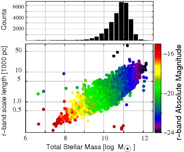
Figure 15: Total stellar mass distribution of our sample is illustrated in the top panel, and the Scale length versus mass diagram shows the expected behaviour in the bottom panel. The colour code shows the $r$-band absolute magnitude derived from the SDSS apparent $r$-band magnitude. The histogram and the scatter plot illustrate the same mass range.

4.3 Scale Length versus Stellar Mass

We retrieve stellar masses for our sample galaxies by cross matching our sample with the publically available sample of Kauffmann et al. (2003) and Brinchmann et al. (2004), and find stellar masses for 30126 (i.e., almost all our sample) galaxies. These authors have calculated total stellar masses for nearly a million SDSS galaxies based on photometry of the outer regions of the galaxies with models that produce dust corrected star formation rates and use upgraded stellar population synthesis spectra for the continuum subtraction. As noted by these authors, comparison between the stellar masses derived from photometry and spectra from the central regions show that the fits to the photometry are more constrained at low mass since the emission line contribution makes the line index fits less well-constrained. Since the spectroscopic masses are based on fibre spectra from SDSS, which cover only a fraction of the galaxies, we opt to use the stellar masses from photometry.

In Fig. 15 we illustrate the scale length as a function of total stellar mass, and find that larger mass galaxies have larger scale lengths. Moreover, we find that this increase is accompanied by a larger spread in scale length. Galaxies with total stellar mass less than $10^{8}\rm{~{}M}_{\odot}$ have average $r$-band scale length of $238\pm 94$ pc, galaxies with total stellar mass between $10^{9}$ and $10^{10}\rm{~{}M}_{\odot}$ have average scale length of $1.52\pm 0.65$ kpc, and galaxies with total stellar mass between $10^{11}$ and $10^{12}\rm{~{}M}_{\odot}$ have average scale length of $5.73\pm 1.94$ kpc. All points in Fig. 15 are also color coded to show the consistently increasing intrinsic absolute magnitude for larger stellar mass galaxies.

5 Discussion

We have derived reliable scale lengths for 30374 disk/spiral galaxies, with no sign of ongoing interaction or disturbed morphology, in all five $u,g,r,i,$ and $z$-bands from SDSS DR6 images. Cross-correlation of the SDSS sample with the LEDA catalogue has enabled us to investigate the variation of the scale lengths for different types of disk/spiral galaxies. Although the typical scale length in $u$-band is 35% larger than that in the $r$-band, the scale lengths in the $g,r,i,$ and $z$-bands are similar and only become smaller on the average for late morphological types. This result remains consistent when using by-eye morphological classification or when using asymmetry parameter, concentration parameter, or velocity dispersion as an indicator for galaxy morphological type. Our sample spans a range of total stellar masses between $10^{6.6}$ and $10^{12.2}\rm{~{}M}_{\odot}$ with a typical galaxy mass of $10^{10.8\pm 0.54}\rm{~{}M}_{\odot}$, and shows that the while scale length increases for more massive galaxies, the scale length spread also increases with galaxy mass. Overall, these results are in full agreement with the recent work by Courteau et al. (2007).

Scale length variations between bands are commonly studied to better understand the content and distribution of different stellar populations, metals, and/or dust. A colour gradient is expected to increase from early-type spirals to late-type spirals, mainly due to extinction, which increases to later types. However, for Scd galaxies or later the colour gradient becomes smaller, because of decreasing amount of extinction (see, e.g., Peletier & Balcells, 1996; de Grijs, 1998).

Changes in galaxy scale length in different wavelengths can be attributed to extinction by moderate amounts of dust, with radial metallicity and age gradients as other contributing factors (Elmegreen & Elmegreen, 1984; Peletier et al., 1994; Beckman et al., 1996). All these parameters will probably change as a function of redshift, enabling us to measure the variation of intrinsic scale length with cosmological epoch. It is expected that the opacity of disk galaxies is expected to have been systematically higher in the past (e.g., Dwek, 1998; Pei et al., 1999). The fact that the observed radial colour vary little suggests strongly that stellar population effects are not important here. Dust effects are studied by using radiative transfer models which take into account scattering as well as absorption by dust, and observationally by investigating the scale length ratio in different bands as a function of inclination, i.e., optical depth. However, there are some degeneracies. Any tendency of the stars in the outer parts of disks to be bluer would tend to result in underestimated dust content. Any tendency of the dust to concentrate towards the centre would result in an overestimate of the bluer scale lengths, and would not be distinguishable photometrically from a tendency of the stars in the outer disc to be bluer (c.f. Pohlen & Trujillo, 2006; Erwin et al., 2008; Azzolini et al., 2008). Peletier et al. (1994, 1995) found that scale length ratios could change, due to stellar population changes, by a factor of approximately 1.1-1.2 from blue to near-infrared ($K$-band). This would correspond to a factor of about 1.03-1.06 from $g$ to $z$. Since these numbers are very small, a very accurate analysis is needed to derive conclusions from the SDSS database. Our results seem to first order in agreement with these numbers.

The derived scale lenghts and our presentation of the transformation coefficients for converting observed scale lengths from one SDSS band to another, furthermore, are meant to be useful tools to test the results of cosmological galaxy formation models, whether numerical, or semi-analytical.

In the future, we plan to add the stored parameters form the Galaxy ZOO project to obtain a larger sample with morphological classifications (at this stage, detailed morphologies are not available), but also compare scale length as a function environment, nuclear activity, and colour gradients (e.g., comparing the sample with that of Hatziminaoglou et al., 2005). Many more parameters can be further investigated, and with the data and the derived parameters at hand, we now have the capability to continue this project in various and potentially unforeseeable directions.

References

- Abraham et al. (1996) Abraham, R. G., van den Bergh, S., Glazebrook, K., Ellis, R. S., Santiago, B. X., Surma, P., Griffiths, R. E. 1996, ApJS, 107, 1
- Adelman-McCarthy et al. (2008) Adelman-McCarthy, J. K. et al. 2008, ApJS, 175, 297
- Aguerri et al. (1998) Aguerri, J. A. L., Beckman, J. E., Prieto, M. 1998, AJ, 116, 2136
- Azzolini et al. (2008) Azzolini, R., Trujillo, I., Beckman, J. E. 2008, ApJ, 679, L69
- Balcells & Peletier (1994) Balcells, M., Peletier, R. F. 1994, AJ, 107, 135
- Baggett et al. (1998) Baggett, W. E., Baggett, S. M., Anderson, K. S. J. 1998, AJ, 116, 1626
- Beckman et al. (1996) Beckman, J. E., Peletier, R. F., Knapen, J. H., Corradi, R. L. M., Gentet, L. J. 1996, ApJ, 467, 175
- Bertin & Arnouts (1996) Bertin, E., Arnouts, S. 1996, A&AS, 117, 393
- Brinchmann et al. (2004) Brinchmann, J. et al. 2004, MNRAS, 351, 1151
- Boroson (1981) Boroson, T. 1981, ApJS, 46, 177
- Bournaud et al. (2007) Bournaud, F., Elmegreen, B. G., Elmegreen, D. M. 2007, ApJ, 670, 237
- Burda & Feitzinger (1992) Burda, P., Feitzinger, J. V. 1992, A&A, 261, 697
- Byun & Freeman (1995) Byun, Y. I., Freeman, K. C. 1995, ApJ, 448, 563
- Ceverino et al. (2010) Ceverino, D., Dekel, A., Bournaud, F. 2010, MNRAS, in press, arXiv:0907.3271
- Combes & Elmegreen (1993) Combes, F., & Elmegreen, B. G. 1993, A&A, 271, 391
- Conselice (1997) Conselice, C. J. 1997, PASP, 109, 1251
- Conselice (2003) Conselice, C. J. 2003, ApJSS, 147, 1
- Conselice et al. (2003) Conselice, C. J., Bershady, M. A., Dickinson, M., Papovich, C. 2003, ApJ, 126, 1183
- Coulais et al. (2009) Coulais, A., Schellens, M., Gales, J., Arabas, S., Boquier, M., Chanial, P., Messmer, P., 2009: Status of GDL - GNU Data Language, Proc. of the 19th conference on Astronomical Data Analysis Software and Systems, Sapporo, Japan
- Courteau (1996) Courteau, S. 1996 ApJS, 103, 363
- Courteau et al. (2007) Courteau, S. et al. 2007, ApJ, 671, 203
- Cunow (1998) Cunow, B. 1998, A&ASS, 129, 593
- Cunow (2001) Cunow, B. 2001, MNRAS, 323, 130
- Cunow (2004) Cunow, B. 2004, MNRAS, 353, 477
- Dalcanton et al. (1997) Dalcanton, J. J., Spergel, D. N., Summers, F. J. 1997, ApJ, 482, 659
- de Grijs (1998) de Grijs, R. 1998, MNRAS, 299, 595
- de Jong (1996) de Jong, R. S. 1996, A&A, 313, 45
- de Vaucouleurs (1948) de Vaucouleurs, G. 1948, AnAp, 11, 247
- de Vaucouleurs et al. (1991) de Vaucouleurs, G., de Vaucouleurs, A., Corwin, H. G., Jr., Buta, R. J., Paturel, G., Fouque, P. 1991, Third Reference Catalogue of Bright Galaxies Volume 1-3, Springer-Verlag: Berlin, Heidelberg, New York
- Doi et al. (1993) Doi, M., Fukugita, M., Okamura, S. 1993, MNRAS, 264, 832
- Dutton (2009) Dutton, A. 2009, MNRAS, 396, 141
- Dwek (1998) Dwek, E. 1998, ApJ, 501, 643
- Elmegreen & Elmegreen (1984) Elmegreen, D. M. & Elmegreen, B. G. 1984, ApJS, 54, 127
- Elmegreen et al. (1996) Elmegreen, B. G. Elmegreen, D. M., Chromey, F. R., Hasselbacher, D. A., Bissell, B. A. 1996, AJ, 111, 2233
- Elmegreen et al. (2005) Elmegreen, B. G., Elmegreen, D. M., Vollbach, D. R., Foster, E. R., Ferguson, T. E. 2005, 634, 101
- Erwin et al. (2008) Erwin, P., Pohlen, M., Beckman, J. E. 2008, AJ, 135, 20
- Fathi & Peletier (2003) Fathi, K., Peletier, R. F. 2003, A&A, 407, 61
- Fathi (2004) Fathi, K. 2004, PhD Thesis, Groningen University
- Freeman (1970) Freeman, K. C. 1970, 160, 811
- Fukugita et al. (2007) Fukugita, M. et al. 2007, AJ, 134, 579
- Giovanelly & Haynes (2002) Giovanelli, R., Haynes, M. 2002, ApJ, 571, L107
- Governato et al. (2010) Governato, F. et al. 2010, Nature, 463, 203
- Graham (2001) Graham, A. W. 2001, AMNRAS, 326, 543
- Graham & de Blok (2001) Graham, A. W., de Blok, W. J. G. 2001, ApJ, 556, 177
- Graham & Worley (2008) Graham, A. W., Worley, C.C. 2008, MNRAS, 388, 1708
- Hatziminaoglou et al. (2005) Hatziminaoglou, E. et al. 2005, MNRAS, 364, 47
- Holwerda (2005) Holwerda, B. 2005, PhD. Thesis, Groningen University
- Simien & de Vaucouleurs (1983) Simien, F. & de Vaucouleurs, G. 1983, IAUS, 100, 375
- Lauberts (1982) Lauberts A. 1982, The ESO/Uppsala Survey of the ESO(B) Atlas, European Southern Observatory
- Lin & Pringle (1987) Lin, D. N. C., Pringle, J. E. 1987, MNRAS, 225, 607
- Loveday (1996) Loveday J. 1996, MNRAS, 278, 1025
- Kauffmann et al. (2003) Kauffmann, G. et al. 2003, MNRAS, 341, 33
- Kent (1985) Kent, S. M. 1985, ApJS, 59, 115
- Knapen (2004) Knapen, J. H. 2004, ”Penetrating Bars Through Masks of Cosmic Dust”, in ASSL, 319, 189
- Knapen & van der Kruit (1991) Knapen, J. H., van der Kruit, P. C. 1991, A&A, 248, 57
- Knezek (1993) Knezek, P. 1993, PhD thesis, University of Massachusetts
- Kormendy & Kennicutt (2004) Kormendy, J. & Kennicutt, Jr., R. C. 2004, ARA&A, 42, 603
- MacArthur (2003) MacArthur, L. A., Courteau, S., Holtzman, J. A. 2003, ApJ, 582, 689
- Martig & Bournaud (2010) Martig, M., Bournaud, F. 2010, ApJ, submitted (arXiv:0911.0891)
- Mo et al. (1998) Mo, H. J., Mao, S., White, S. D. 1998, MNRAS, 295, 319
- Mosteller & Tukey (1977) Mosteller, F., Tukey, J. 1977, Data Analysis and Regression, Addison-Wesley
- Nilson (1973) Nilson P. 1973, Uppsala General Catalogue of Galaxies, Uppsala Astr. Obs. Annaler, Band 6
- Paturel et al. (2003) Paturel, G., Petit, C., Prugniel, P., Theureau, G., Rousseau, J., Brouty, M., Dubois, P., Cambrésy, L. 2003, A&A, 412, 45
- Pei et al. (1999) Pei, Y. C., Fall, S. M., Hauser, M. G. 1999, ApJ, 522, 604
- Peletier et al. (1994) Peletier, R. F., Valentijn, E. A., Moorwood, A. F. M., Freudling, W. 1994, A&AS, 108, 621
- Peletier et al. (1995) Peletier, R. F., Valentijn, E. A., Moorwood, A. F. M., Freudling, W., Knapen, J. H., Beckman, J. E. 1995, A&A, 300, L1
- Peletier & Balcells (1996) Peletier, R. F., Balcells, M. 1996, in ”Spiral Galaxies in the Near-IR”, ESO/MPA proceedings, eds: Dante Minniti and Hans-Walter Rix, Springer-Verlag Berlin Heidelberg New York
- Prieto et al. (2001) Prieto, M., Aguerri, J. A. L.. Varela, A. M.. Muñoz-Tuñn, C. 2001, A&A, 367, 405
- Pohlen & Trujillo (2006) Pohlen, M., Trujillo, I. A&A, 454, 759
- Romanishin et al. (1983) Romanishin, W., Strom, K. M., Strom, S. E. 1983, ApJS, 53, 105
- Sandage (1961) Sandage, A. 1961, The Hubble Atlas of Galaxies, Washington: Carnegie Institute Washington
- Schade et al. (1995) Schade, D., Lilly, S. J., Crampton, D., Hammer, F., Le Fevre, O., Tresse, L. 1995, ApJ, 451, L1
- Schaye et al. (2010) Schaye, J. et al. 2010, MNRAS, 402, 1536
- Schombert et al. (1992) Schombert, J. M. Bothun, G. D., Schneider, S. E., McGaugh, S. S. 1992, AP, 103, 1107
- Sérsic (1968) Sérsic, J. L. 1968, Atlas de galaxias australes, Observatorio Astronomico Cordoba
- Shimasaku et al. (2001) Shimasaku, K. et al. 2001, AJ, 122, 1238
- Silk (2001) Silk, J. 2001, MNRAS, 324, 313
- Valentijn (1990) Valentijn, E. A. 1990, Nature, 346, 153
- van der Kruit (1987) van der Kruit, P. C. 1987, A&A, 173, 59
- van Driel et al. (1995) van Driel, W. Valentijn, E. A., Wesselius, P. R., Kussendrager, D. 1995, A&A, 298, 41
- Vorontsov-Velyaminov et al. (1963) Vorontsov-Velyaminov B.A., Arkipova V.P., Kranogorskaja A.A.n 1963-1974, Morphological Catalogue of Galaxies, Trudy Sternberg Stat. Astr.Inst. 32,33,34
- Yamauchi et al. (2005) Yamauchi, C. et al. 2005, ApJ, 130, 1545
- York et al. (2000) York, D. G. et al. 2000, AJ, 120, 1579