Turaev-Viro invariants as an extended TQFT

Abstract.

In this paper we show how one can extend Turaev-Viro invariants, defined for an arbitrary spherical fusion category $\mathcal{C}$, to 3-manifolds with corners. We demonstrate that this gives an extended TQFT which conjecturally coincides with the Reshetikhin-Turaev TQFT corresponding to the Drinfeld center $Z(\mathcal{C})$. In the present paper we give a partial proof of this statement.

Introduction

Turaev–Viro (TV) invariants of 3-manifolds $Z_{TV}(M)$ were defined by Turaev and Viro in TV using a quantum analog of 6j symbols for $sl_{2}$. In the same paper it was shown that these invariants can be extended to a 3-dimensional TQFT.

Later, Barrett and Westbury barrett showed that these invariants can be defined for any monoidal category $\mathcal{C}$ possessing a suitable notion of duality (“spherical category”). In particular, they can be defined for the category of $G$-graded vector spaces, where $G$ is a finite group. In this special case, the resulting TQFT coincides with the version of Chern–Simons theory with the finite gauge group $G$, described in freed-quinn (or in more modern language, in FHLT); in physics literature, this theory is also known as the Levin–Wen model.

In the case when the category $\mathcal{C}$ is not only monoidal but in fact modular (in particular, braided), there is another 3-dimensional TQFT based on $\mathcal{C}$, namely Reshetikhin–Turaev TQFT. It was shown in turaev that in this case, one has

$$Z_{TV,\mathcal{C}}(M)=Z_{RT,\mathcal{C}}(M)Z_{RT,\mathcal{C}}(\overline{M})$$

where $\overline{M}$ is $M$ with opposite orientation. In particular, if $\mathcal{C}$ is unitary category over $\mathbb{C}$, then $Z_{TV,\mathcal{C}}(M)=|Z_{RT,\mathcal{C}}(M)|^{2}$.

It has been conjectured that in the general case, when $\mathcal{C}$ is a spherical (but not necessarily modular) category, one has

$$Z_{TV,\mathcal{C}}(M)=Z_{RT,Z(\mathcal{C})}(M)$$

where $Z(\mathcal{C})$ is the so-called Drinfeld center of $\mathcal{C}$ (see Section 2); moreover, this extends to an isomorphism of the corresponding TQFTs. Some partial results in this direction can be found, for example, in muger2; however, the full statement remained a conjecture.

The current paper is the first in a series giving a proof of this conjecture for an arbitrary spherical category $\mathcal{C}$ over an algebraically closed field $\mathbf{k}$ of characteristic zero. In the current paper, we extend TV invariants to 3-manifolds with corners of codimension 2 (or, which is closely related, to 3-manifolds with framed tangles inside); in the language of lurie, we construct a 3-2-1 extension of TV theory. This extension satisfies $Z_{TV}(S^{1})=Z(\mathcal{C})$: boundary circles of 2-surfaces should be colored by objects of $Z(\mathcal{C})$. We also show that for an $n$-punctured sphere, the resulting vector space coming from this extended TV theory coincides with the one coming from Reshetikhin-Turaev theory based on $Z(\mathcal{C})$.

Thsi extended theory is related to the one suggested in turaev94; however, that paper only considered the case when $\mathcal{C}$ itself is modular and the components of links are labeled by objects of $\mathcal{C}$, not $\mathbb{Z}(\mathcal{C})$. We will investigate the relation between these constructions in forthcoming papers.

After the preliminary version of this paper was posted, a proof of formula $Z_{TV,\mathcal{C}}(M)=Z_{RT,Z(\mathcal{C})}(M)$ was announced by Turaev turaev-conference; howevere, details of this proof are not yet available.

Acknowledgments

The authors would like to thank Oleg Viro, Victor Ostrik, Kevin Costello and Owen Gwilliam for helpful suggestions and discussions.

1. Preliminaries I: spherical categories

In this section we collect notation and some facts about spherical categories.

We fix an algebraically closed field $\mathbf{k}$ of characteristic 0 and denote by $\mathcal{V}ec$ the category of finite-dimensional vector spaces over $\mathbf{k}$.

Throughout the paper, $\mathcal{C}$ will denote a spherical fusion category over $\mathbf{k}$. We refer the reader to the paper drinfeld for the definitions and properties of such categories. Note that we are not requiring a braiding on $\mathcal{C}$.

In particular, $\mathcal{C}$ is semisimple with finitely many isomorphism classes of simple objects. We will denote by $\operatorname{Irr}(\mathcal{C})$ the set of isomorphism classes of simple objects. We will also denote by $\mathbf{1}$ the unit object in $\mathcal{C}$ (which is simple).

Two main examples of spherical categories are the category $\mathcal{V}ec^{G}$ of finite-dimensional $G$-graded vector spaces (where $G$ is a finite group) and the category $\operatorname{Rep}(U_{q}\mathfrak{g})$ which is the semisimple part of the category of representations of a quantum group $U_{q}\mathfrak{g}$ at a root of unity; this last category is actually modular, but we will not be using this.

To simplify the notation, we will assume that $\mathcal{C}$ is a strict pivotal category, i.e. that $V^{**}=V$. As is well-known, this is not really a restriction, since any pivotal category is equivalent to a strict pivotal category.

We will denote, for an object $X$ of $\mathcal{C}$, by

$$d_{X}=\dim X\in\mathbf{k}$$

its categorical dimension; it is known that for simple $X$, $d_{X}$ is non-zero. We will fix, for any simple object $X_{i}\in\mathcal{C}$, a choice of square root $\sqrt{d_{X}}$ so that for $X=\mathbf{1}$, $\sqrt{d_{\mathbf{1}}}=1$ and that for any simple $X$, $\sqrt{d_{X}}=\sqrt{d_{X^{*}}}$.

We will also denote

(1.1) $$\mathcal{D}=\sqrt{\sum_{x\in\operatorname{Irr}(\mathcal{C})}d_{X}^{2}}$$

(throughout the paper, we fix a choice of the square root). Note that by results of ENO, $\mathcal{D}\neq 0$.

We define the functor $\mathcal{C}^{\boxtimes n}\to\mathcal{V}ec$ by

(1.2) $$\langle V_{1},\dots,V_{n}\rangle=\operatorname{Hom}_{\mathcal{C}}(\mathbf{1},V_{1}\otimes\dots\otimes V_{n})$$

for any collection $V_{1},\dots,V_{n}$ of objects of $\mathcal{C}$. Note that pivotal structure gives functorial isomorphisms

(1.3) $$z\colon\langle V_{1},\dots,V_{n}\rangle\simeq\langle V_{n},V_{1},\dots,V_{n-1}\rangle$$

such that $z^{n}=\operatorname{id}$ (see BK*Section 5.3); thus, up to a canonical isomorphism, the space $\langle V_{1},\dots,V_{n}\rangle$ only depends on the cyclic order of $V_{1},\dots,V_{n}$.

We have a natural composition map

(1.4) $$\langle V_{1},\dots,V_{n},X\rangle\otimes\langle X^{*},W_{1},\dots,W_{m}\rangle \to\langle V_{1},\dots,V_{n},W_{1},\dots,W_{m}\rangle$$

$$\varphi\otimes\psi\mapsto\varphi\underset{\scriptstyle X}{\circ}\psi=\operatorname{ev}_{X}\circ(\varphi\otimes\psi)$$

where $\operatorname{ev}_{X}\colon X\otimes X^{*}\to\mathbf{1}$ is the evaluation morphism. It follows from semisimplicity of $\mathcal{C}$ that direct sum of these composition maps gives a functorial isomorphism

(1.5) $$\bigoplus_{X\in\operatorname{Irr}(\mathcal{C})}\langle V_{1},\dots,V_{n},X\rangle\otimes\langle X^{*},W_{1},\dots,W_{m}\rangle\simeq\langle V_{1},\dots,V_{n},W_{1},\dots,W_{m}\rangle.$$

Note that for any objects $A,B\in\operatorname{Obj}\mathcal{C}$, we have a non-degenerate pairing $\operatorname{Hom}_{\mathcal{C}}(A,B)\otimes\operatorname{Hom}_{\mathcal{C}}(A^{*},B^{*})\to\mathbf{k}$ defined by

(1.6) $$(\varphi,\varphi^{\prime})=(\mathbf{1}\xrightarrow{\operatorname{coev}_{A}}A\otimes A^{*}\xrightarrow{\varphi\otimes\varphi^{\prime}}B\otimes B^{*}\xrightarrow{\operatorname{ev}_{B}}\mathbf{1})$$

In particular, this gives us a non-degenerate pairing $\langle V_{1},\dots,V_{n}\rangle\otimes\langle V_{n}^{*},\dots,V_{1}^{*}\rangle\to\mathbf{k}$ and thus, functorial isomorphisms

(1.7) $$\langle V_{1},\dots,V_{n}\rangle^{*}\simeq\langle V_{n}^{*},\dots,V_{1}^{*}\rangle$$

compatible with the cyclic permutations (1.3).

We will frequently use graphical representations of morphisms in the category $\mathcal{C}$, using tangle diagrams as in turaev or BK. However, our convention is that of BK: a tangle with $k$ strands labeled $V_{1},\dots,V_{k}$ at the bottom and $n$ strands labeled $W_{1},\dots,W_{n}$ at the top is considered as a morphism from $V_{1}\otimes\dots\otimes V_{k}\to W_{1}\otimes\dots\otimes W_{n}$. As usual, by default all strands are oriented going from the bottom to top. Note that since $\mathcal{C}$ is assumed to be a spherical category and not a braided one, no crossings are allowed in the diagrams.

For technical reasons, it is convenient to extend the graphical calculus by allowing, in addition to rectangular coupons, also circular coupons labeled with morphisms $\varphi\in\langle V_{,}1\dots,V_{n}\rangle$. This is easily seen to be equivalent to the original formalism: every such circular coupon can be replaced by the usual rectangular one as shown in Figure 1.

=

Figure 1. Round coupons

We will also use the following convention: if a figure contains a pair of circular coupons, one with outgoing edges labeled $V_{1},\dots,V_{n}$ and the other with edges labeled $V_{n}^{*},\dots,V_{1}^{*}$ , and the coupons are labeled by pair of letters $\varphi,\varphi^{*}$ (or $\psi,\psi^{*}$, or …) it will stand for summation over the dual bases:

(1.8) $$\leavevmode\hbox to143.13pt{\vbox to52.4pt{\text{[drawing]}}}\quad=\sum_{\alpha}\quad\leavevmode\hbox to143.13pt{\vbox to52.4pt{\text{[drawing]}}} \varphi V_{1} V_{n} \varphi^{*} V_{n}^{*} V_{1}^{*} \varphi_{\alpha} V_{1} V_{n} \varphi^{\alpha} V_{n}^{*} V_{1}^{*}$$

where $\varphi_{\alpha}\in\langle V_{1},\dots,V_{n}\rangle$, $\varphi^{\alpha}\in\langle V_{n}^{*},\dots,V_{1}^{*}\rangle$ are dual bases with respect to pairing (1.6).

The following lemma, proof of which is left to the reader, lists some properties of this pairing and its relation with the composition maps (1.4).

Lemma 1.1.

1. If $X$ is simple and $\varphi\in\langle X,A\rangle$, $\varphi^{\prime}\in\langle A^{*},X^{*}\rangle$ then

   $$\raisebox{-0.5pt}{\includegraphics{figures/pair1.eps}}=\frac{(\varphi,\varphi^{\prime})}{d_{X}}\quad\raisebox{-0.5pt}{\includegraphics{figures/pair2.eps}}$$

2. $$\sum_{i\in\operatorname{Irr}(\mathcal{C})}d_{i}\leavevmode\hbox to99.38pt{\vbox to49.64pt{\text{[drawing]}}}=\leavevmode\hbox to85.75pt{\vbox to58.16pt{\text{[drawing]}}} \varphi \varphi^{*} \dots \dots V_{1} V_{n} V_{n} V_{1} X_{i} \dots \dots V_{1} V_{n} \varphi \varphi^{*} \dots \dots V_{1} V_{n} V_{n} V_{1} X_{i} \dots \dots V_{1} V_{n}$$

   (we use here convention (1.8)).

3. If $X$ is simple, $\varphi\in\langle A,X\rangle$, $\varphi^{\prime}\in\langle X^{*},A^{*}\rangle$, $\psi\in\langle X^{*},B\rangle$, $\psi^{\prime}\in\langle B^{*},X\rangle$, then

   (1.9) $$(\varphi\underset{\scriptstyle X}{\circ}\psi,\psi^{\prime}\underset{\scriptstyle X^{*}}{\circ}\varphi^{\prime})=\frac{1}{d_{X}}(\varphi,\varphi^{\prime})(\psi^{\prime},\psi)$$

   (see Figure 2).

   $$\raisebox{-0.5pt}{\includegraphics{figures/compL.eps}}=\frac{(\varphi,\varphi^{\prime})}{d_{X}}\raisebox{-0.5pt}{\includegraphics{figures/compR.eps}}=\frac{(\varphi,\varphi^{\prime})(\psi^{\prime},\psi)}{d_{X}}$$

   Figure 2. Compatibility of pairing with composition.

Corollary 1.2.

Let $X$ be a simple object. Define the rescaled composition map

(1.10) $$\langle V_{1},\dots,V_{n},X\rangle\otimes\langle X^{*},W_{1},\dots,W_{m}\rangle \to\langle V_{1},\dots,V_{n},W_{1},\dots,W_{m}\rangle$$

$$\varphi\otimes\psi \mapsto\varphi\underset{\scriptstyle X}{\bullet}\psi=\sqrt{d_{X}}\ \operatorname{ev}_{X}\circ(\varphi\otimes\psi)$$

Then the rescaled composition map agrees with the pairing:

$$(\varphi\underset{\scriptstyle X}{\bullet}\psi,\psi^{\prime}\underset{\scriptstyle X^{*}}{\bullet}\varphi^{\prime})=(\varphi,\varphi^{\prime})(\psi^{\prime},\psi)$$

(same notation as in (1.9)).

The following result, which easily follows from Lemma 1.1, will also be very useful.

Lemma 1.3.

If the subgraphs $A$, $B$ are not connected, then

$$\leavevmode\hbox to167.56pt{\vbox to45.67pt{\text{[drawing]}}}=\leavevmode\hbox to139.1pt{\vbox to58.63pt{\text{[drawing]}}} A \varphi \varphi^{*} B V_{1} V_{n} V_{1} V_{n} A B V_{1} V_{n} A \varphi \varphi^{*} B V_{1} V_{n} V_{1} V_{n} A B V_{1} V_{n}$$

Finally, we will need the following result, which is the motivation for the name “spherical category”.

Let $\Gamma$ be an oriented graph embedded in the sphere $S^{2}$, where each edge $e$ is colored by an object $V(e)\in\mathcal{C}$, and each vertex $v$ is colored by a morphism $\varphi_{v}\in\langle V(e_{1})^{\pm},\dots V(e_{n})^{\pm}\rangle$, where $e_{1},\dots,e_{n}$ are the edges adjacent to vertex $v$, taken in clockwise order, and $V(e_{i})^{\pm}=V(e_{i})$ if $e_{i}$ is outgoing edge, and $V^{*}(e_{i})$ if $e_{i}$ is the incoming edge.

By removing a point from $S^{2}$ and identifying $S^{2}\setminus{pt}\simeq\mathbb{R}^{2}$, we can consider $\Gamma$ as a planar graph. Replacing each vertex $v$ by a circular coupon labeled by morphism $\varphi_{v}$ as shown in Figure 3, we get a graph of the type discussed above and which therefore defines a number $Z_{RT}(\Gamma)\in\mathbf{k}$ (see, e.g., BK or turaev).

    

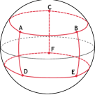
Figure 3. Graph on a sphere and its “flattening” to the plane

Theorem 1.4.

barrett The number $Z_{RT}(\Gamma)\in\mathbf{k}$ does not depend on the choice of a point to remove from $S^{2}$ or on the choice of order of edges at vertices compatible with the given cyclic order and thus defines an invariant of colored graphs on the sphere.

2. Preliminaries II: Drinfeld Center

We will also need the notion of Drinfeld center of a spherical fusion category. Recall that the Drinfeld center $Z(\mathcal{C})$ of a fusion category $\mathcal{C}$ is defined as the category whose objects are pairs $(Y,\varphi_{Y})$, where $Y$ is an object of $\mathcal{C}$ and $\varphi_{Y}$ – a functorial isomorphism $Y\otimes-\to-\otimes Y$ satisfying certain compatibility conditions (see muger1).

As before, we will frequently use graphical presentation of morphisms which involve objects both of $\mathcal{C}$ and $Z(\mathcal{C})$. In these diagrams, we will show objects of $Z(C)$ by double green lines and the half-braiding isomorphism $\varphi_{Y}\colon Y\otimes V\to V\otimes Y$ by crossing as in Figure 4.

Figure 4. Graphical presentation of the half-braiding $\varphi_{Y}\colon Y\otimes V\to V\otimes Y$, $Y\in\operatorname{Obj}Z(\mathcal{C})$, $V\in\operatorname{Obj}\mathcal{C}$

We list here main properties of $Z(\mathcal{C})$, all under the assumption that $\mathcal{C}$ is a spherical fusion category over an algebraically closed field of characteristic zero.

Theorem 2.1.

muger2 $Z(\mathcal{C})$ is a modular category; in particular, it is semisimple with finitely many simple objects, it is braided and has a pivotal structure which coincides with the pivotal structure on $\mathcal{C}$.

We have an obvious forgetful functor $F\colon Z(\mathcal{C})\to\mathcal{C}$. To simplify the notation, we will frequently omit it in the formulas, writing for example $\operatorname{Hom}_{\mathcal{C}}(Y,V)$ instead of $\operatorname{Hom}_{\mathcal{C}}(F(Y),V)$, for $Y\in\operatorname{Obj}Z(\mathcal{C})$, $V\in\operatorname{Obj}\mathcal{C}$. Note, however, that if $Y,Z\in\operatorname{Obj}Z(\mathcal{C})$, then $\operatorname{Hom}_{Z(\mathcal{C})}(Y,Z)$ is different from $\operatorname{Hom}_{\mathcal{C}}(Y,Z)$: namely, $\operatorname{Hom}_{Z(\mathcal{C})}(Y,Z)$ is a subspace in $\operatorname{Hom}_{\mathcal{C}}(Y,Z)$ consisting of those morphisms that commute the with the half-braiding. The following lemma will be useful in the future.

Lemma 2.2.

Let $Y,Z\in\operatorname{Obj}Z(\mathcal{C})$. Define the operator

$P\colon\operatorname{Hom}_{\mathcal{C}}(Y,Z)\to\operatorname{Hom}_{\mathcal{C}}(Y,Z)$ by the following formula:

$$P\psi=\frac{1}{\mathcal{D}^{2}}\sum_{X\in\operatorname{Irr}(\mathcal{C})}d_{X}\quad\leavevmode\hbox to53.59pt{\vbox to87.98pt{\text{[drawing]}}} \psi Y Z X \psi Y Z X$$

Then $P$ is a projector onto the subspace $\operatorname{Hom}_{Z(\mathcal{C})}(Y,Z)\subset\operatorname{Hom}_{\mathcal{C}}(Y,Z)$.

Proof.

It is immediate from the definition that if $\psi\in\operatorname{Hom}_{Z(\mathcal{C})}(Y,Z)$, then $P\psi=\psi$. On the other hand, using Lemma 1.1, we get that for any $\psi\in\operatorname{Hom}_{\mathcal{C}}(Y,Z)$, one has $(P\psi)\varphi_{Y}=\varphi_{Z}(P\psi)$:

$$(P\psi)\varphi_{Y} =\frac{1}{\mathcal{D}^{2}}\sum_{j}d_{j}\quad\leavevmode\hbox to85.37pt{\vbox to108.12pt{\text{[drawing]}}}=\frac{1}{\mathcal{D}^{2}}\sum_{i,j}d_{i}d_{j}\quad\leavevmode\hbox to70.35pt{\vbox to104.23pt{\text{[drawing]}}} \psi Y Z j W \psi Y Z \varphi \varphi^{*} j i W W \psi Y Z j W \psi Y Z \varphi \varphi^{*} j i W W$$

$$=\frac{1}{\mathcal{D}^{2}}\sum_{i}d_{i}\quad\leavevmode\hbox to83.46pt{\vbox to108.12pt{\text{[drawing]}}}=\varphi_{Z}(P\psi), \psi Y Z i W \psi Y Z i W$$

(as before, we are using convention (1.8)). ∎

The following theorem is a refinement of ENO*Proposition 5.4.

Theorem 2.3.

Let $F\colon Z(\mathcal{C})\to\mathcal{C}$ be the forgetful functor and $I\colon\mathcal{C}\to Z(\mathcal{C})$ the (left) adjoint of $F$: $\operatorname{Hom}_{Z(\mathcal{C})}(I(V),X)=\operatorname{Hom}_{\mathcal{C}}(V,F(X))$. Then for $V\in\operatorname{Obj}\mathcal{C}$, one has

(2.1) $$I(V)=\bigoplus_{i\in\operatorname{Irr}(\mathcal{C})}X_{i}\otimes V\otimes X_{i}^{*}$$

with the half braiding given by

$$\bigoplus_{i,j\in\operatorname{Irr}(\mathcal{C})}\sqrt{d_{i}}\sqrt{d_{j}}\quad\leavevmode\hbox to68.89pt{\vbox to104.97pt{\text{[drawing]}}} V \varphi \varphi^{*} i j W i j W V \varphi \varphi^{*} i j W i j W$$

Figure 5. Half-braiding $I(V)\otimes W\to W\otimes I(V)$.

Note that instead of normalizing factor $\sqrt{d_{i}}\sqrt{d_{j}}$ we could have used $d_{i}$ or $d_{j}$ — each of this would give an equivalent definition.

Proof.

Denote $Y=\bigoplus_{i\in\operatorname{Irr}(\mathcal{C})}X_{i}\otimes V\otimes X_{i}^{*}$. It follows from Lemma 1.1 that the morphisms $Y\otimes W\to W\otimes Y$ defined by Figure 5 satisfy the compatibility relations required of half braiding and thus define on $Y$ a structure of an object of $Z(\mathcal{C})$. Now, define for any $Z\in\operatorname{Obj}Z(\mathcal{C})$, maps

$$\operatorname{Hom}_{Z(\mathcal{C})}(Y,Z) \to\operatorname{Hom}_{\mathcal{C}}(V,Z)$$

$$\Psi \mapsto\Psi\circ P_{0}=\quad\leavevmode\hbox to25.94pt{\vbox to81.12pt{\text{[drawing]}}} \Psi V \mathbf{1} \mathbf{1} Z$$

where $P_{0}$ is the embedding $V=\mathbf{1}\otimes V\otimes\mathbf{1}\to Y=\bigoplus X_{i}\otimes V\otimes X_{i}^{*}$ and

$$\operatorname{Hom}_{\mathcal{C}}(V,Z) \to\operatorname{Hom}_{Z(\mathcal{C})}(Y,Z)$$

$$\Phi \mapsto\bigoplus_{i\in\operatorname{Irr}(\mathcal{C})}\sqrt{d_{i}}\leavevmode\hbox to53.09pt{\vbox to69.24pt{\text{[drawing]}}} \Phi V Z i \Phi V Z i$$

It follows from Lemma 2.2 that these two maps are inverse to each other. Composition in one direction is easy. First suppose $\Phi\in\operatorname{Hom}_{\mathcal{C}}(V,Z)$. The computation is shown below.

$$\Phi\to\bigoplus_{i}\sqrt{d_{i}}\quad\leavevmode\hbox to53.09pt{\vbox to69.24pt{\text{[drawing]}}}\to\Phi. \Phi V Z i \Phi V Z i$$

The composition in opposite order is as follows:

$$\Psi\to\leavevmode\hbox to25.94pt{\vbox to81.12pt{\text{[drawing]}}}\to\bigoplus_{i}\sqrt{d_{i}}\leavevmode\hbox to53.09pt{\vbox to82.24pt{\text{[drawing]}}}=\bigoplus_{i}\sqrt{d_{i}}\sqrt{d_{j}}\leavevmode\hbox to48.38pt{\vbox to84.8pt{\text{[drawing]}}}=\leavevmode\hbox to17.98pt{\vbox to81.12pt{\text{[drawing]}}} \Psi V \mathbf{1} \mathbf{1} Z \Psi V Z i \mathbf{1} \mathbf{1} \Psi \varphi \varphi* V Z i i j^{*} \mathbf{1} j \mathbf{1} \Psi V Z \Psi V \mathbf{1} \mathbf{1} Z \Psi V Z i \mathbf{1} \mathbf{1} \Psi \varphi \varphi* V Z i i j^{*} \mathbf{1} j \mathbf{1} \Psi V Z$$

The first equality holds by functoriality of the half-braiding and Figure 5. The second equality is obvious. Therefore, the two maps are inverses to one another and we have $\operatorname{Hom}_{Z(\mathcal{C})}(Y,Z)=\operatorname{Hom}_{\mathcal{C}}(V,Z)$; thus, $Y=I(V)$. ∎

An easy generalization of Theorem 1.4 allows us to consider graphs in which some of the edges are labeled by objects of $Z(\mathcal{C})$.

Let $\hat{\Gamma}$ be a graph which consists of a usual graph $\Gamma$ embedded in $S^{2}$ as in Theorem 1.4 and a finite collection of non-intersecting oriented arcs $\gamma_{i}$ such that endpoints of each arc $\gamma$ are vertices of graph $\Gamma$, and each vertex has a neighborhood in which arcs $\gamma_{i}$ do not intersect edges of $\Gamma$; however, arcs $\gamma_{i}$ are allowed to intersect edges of $\Gamma$ away from vertices. Note that this implies that for each vertex $v$, we have a natural cyclic order on the set of all edges of $\hat{\Gamma}$ (including arcs $\gamma_{i}$) adjacent to $v$.

Let us color such diagram, labeling each edge of $\Gamma$ by an object of $\mathcal{C}$, each arc $\gamma$ by an object of $Z(\mathcal{C})$, and each vertex $v$ by a vector $\varphi_{v}\in\langle V^{\pm}(e_{1}),\dots,V^{\pm}(e_{n})\rangle$ where $e_{1},\dots,e_{n}$ are edges of $\hat{\Gamma}$ adjacent to $v$ (including the arcs $\gamma_{i}$), and the signs are chosen as in Theorem 1.4.

  

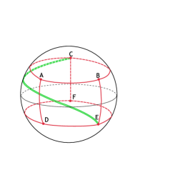
Figure 6. Diagram $\hat{\Gamma}$ on the sphere and its flattening to the plane. Arc $\gamma$ is shown by a double line.

As before, by removing a point from $S^{2}$ and choosing a linear order of edges (including the arcs) at every vertex, we get a diagram in the plane; however, now the projections of arcs $\gamma_{i}$ can intersect edges of $\Gamma$ as shown in Figure 6. Let us turn this into a tangle diagram by replacing each intersection by a picture where the arch $\gamma_{i}$ goes under the edges of $\Gamma$, as shown in Figure 6.

Such a diagram defines a number $Z_{RT}(\hat{\Gamma})$ defined in the usual way, with the extra convention shown in Figure 4.

Theorem 2.4.

The number $Z_{RT}(\hat{\Gamma})\in\mathbf{k}$ does not depend on the choice of a point to remove from $S^{2}$ orand thus defines an invariant of colored graphs on the sphere. Moreover, this number is invariant under homotopy of arcs $\gamma_{i}$.

Proof.

The fact that it is independent of the choice of point to remove and thus is an invariant of a graph on the sphere immediately follows from Theorem 1.4: replacing every crossing by a coupon colored by half-braiding $\varphi_{Y}$ gives a graph as in Theorem 1.4. Invariance under homotopy of arcs $\gamma$ follows from compatibility conditions on half-braiding shown in Figure 7.

=  

Figure 7. Invariance under homotopy

∎

Finally, we will need one more useful construction.

For any $Y\in\operatorname{Obj}Z(\mathcal{C})$, we define a functor functor $\mathcal{C}^{\boxtimes n}\to\mathcal{V}ec$ by

(2.2) $$\langle V_{1},\dots,V_{n}\rangle_{Y}=\operatorname{Hom}_{\mathcal{C}}(\mathbf{1},Y\otimes V_{1}\otimes\dots\otimes V_{n})$$

for any collection $V_{1},\dots,V_{n}$ of objects of $\mathcal{C}$. As before, we have functorial isomorphisms

(2.3) $$z_{Y}\colon\langle V_{1},\dots,V_{n}\rangle_{Y}\simeq\langle V_{n},V_{1},\dots,V_{n-1}\rangle_{Y}$$

obtained as composition

$$\langle Y,V_{1},\dots,V_{n}\rangle\to\langle V_{n},Y,V_{1},\dots,V_{n-1}\rangle\to\langle Y,V_{n},V_{1},\dots,V_{n-1}\rangle$$

(the first isomorphism is the cyclic isomorphism (1.3), the second one is the inverse of half-braiding $\varphi_{Y}$). Note however that in general we do not have $z_{Y}^{n}=\operatorname{id}$.

3. Polytope decompositions

It will be convenient to rewrite the definition of Turaev–Viro (TV) invariants using not just triangulations, but more general cellular decompositions. In this section we give precise definitions of these decompositions.

In what follows, the word “manifold” denotes a compact, oriented, piecewise-linear (PL) manifold; unless otherwise specified, we assume that it has no boundary. Note that in dimensions 2 and 3, the category of PL manifolds is equivalent to the category of topological manifolds. For an oriented manifold $M$, we will denote by $\overline{M}$ the same manifold with opposite orientation, and by $\partial M$, the boundary of $M$ with induced orientation.

Instead of triangulated manifolds as in barrett, we prefer to consider more general cellular decompositions, allowing individual cells to be arbitrary polytopes (rather than just simplices); moreover, we will allow the attaching maps to identify some of the boundary points, for example gluing polytopes so that some of the vertices coincide. On the other hand, we do not want to consider arbitrary cell decompositions (as is done, say, in oeckl), since it would make describing the elementary moves between two such decompositions more complicated. The following definition is the compromise; for lack of a better word, we will call such decompositions polytope decompositions.

Recall that a cellular decomposition of a manifold $M$ is a collection of inclusion maps $B^{d}\to M$, where $B^{d}$ is the (open) $d$-dimensional ball, satisfying certain conditions. Equivalently, we can replace $d$-dimensional balls with $d$-dimensional cubes $I^{d}=(0,1)^{d}$. For a PL manifold, we will call such a cellular decomposition a PL decomposition if each inclusion map $(0,1)^{d}\to M$ is a PL map. In particular, every triangulation of a PL manifold gives such a cellular decomposition (each $d$-dimensional simplex is PL homeomorphic to a $d$-dimensional cube).

We will call a cell regular if the corresponding map $(0,1)^{d}\to M$ extends to a map of the closed cube $[0,1]^{d}\to M$ which is a homeomorphism onto its image.

Definition 3.1.

A polytope decomposition of a 2- or 3-dimensional PL manifold $M$ (possibly with boundary) is a cellular decomposition which can be obtained from a triangulation by a sequence of moves M1—M3 below (for $\dim M=2$, only moves M1, M2).

M1: removing a vertex:

Let $v$ be a vertex which has a neighborhood whose intersection with the 2-skeleton is homeomorphic to the “open book” shown below with $k\geq 1$ leaves; moreover, assume that all leaves in the figure are distinct 2-cells and the two 1-cells are also distinct (i.e., not two ends of the same edge). Then move M1 removes vertex $v$ and replaces two 1-cells adjacent to it with a single 1-cell.

$$\raisebox{-0.5pt}{\includegraphics[scale={0.7}]{figures/M1a.eps}}\xrightarrow{\text{remove vertex }v}\raisebox{-0.5pt}{\includegraphics[scale={0.7}]{figures/M1b.eps}}$$

Figure 8. Move M1

M2: removing an edge:

Let $e$ be a 1-cell which is regular and which is adjacent to exactly two distinct 2-cells $c_{1},c_{2}$ as shown in the figure below. Then the move M2 removes the edge $e$ and replaces the cells $c_{1},c_{2}$ with a single cell $c$.

$$\raisebox{-0.5pt}{\includegraphics[scale={0.7}]{figures/M2a.eps}}\xrightarrow{\text{remove edge }e}\raisebox{-0.5pt}{\includegraphics[scale={0.7}]{figures/M2b.eps}}$$

Figure 9. Move M2

M3: removing a 2-cell:

Let $c$ be a 2-cell which is regular and which is adjacent to exactly two distinct 3-cells $F_{1},F_{2}$ as shown in the figure below. Then the move M2 removes the 2-cell $c$ and replaces the cells $F_{1},F_{2}$ with a single cell $F$.

$$\raisebox{-0.5pt}{\includegraphics[scale={0.7}]{figures/M3a.eps}}\xrightarrow{\text{remove face }c}\raisebox{-0.5pt}{\includegraphics[scale={0.7}]{figures/M3b.eps}}$$

Figure 10. Move M3

A 2 or 3-dimensional PL manifold $M$ with boundary together with a choice of polytope decomposition will be called a combinatorial manifold; for $\dim M=2$, we will also use the term “combinatorial surface”. We will use script letters to denote combinatorial manifolds and Roman letters for underlying PL manifolds.

Note that the extension of the inclusion maps $(0,1)^{d}\to M$ to the boundary does not have to be injective.

If $F$ is an oriented $d$-dimensional cell of a combinatorial manifold $\mathcal{M}$ (i.e., a pair consisting of a cell and its orientation), we can define its boundary $\partial F$ in the obvious way, as a formal union of oriented $(d-1)$-dimensional cells. Note that $\partial F$ can contain the same (unoriented) cell $C$ more than once: for example, one could have $\partial F=\dots\cup C\cup\overline{C}\dots$.

Lemma 3.2.

If $\mathcal{M}$ is a combinatorial manifold of dimension $d$ with boundary, then

$$\bigcup_{F}\partial F=\Bigl{(}\bigcup_{C\in\partial M}C\Bigr{)}\cup\Bigl{(}\bigcup_{c_{in}}c^{\prime}_{in}\cup c^{\prime\prime}_{in}\Bigr{)}$$

where $F$ runs over the set of $d$-cells of $M$ (each taken with induced orientation), $C$ runs over the set of $(d-1)$-cells of $\partial M$ (each taken with induced orientation), and $c_{in}$ runs over the set of (unoriented) $(d-1)$-cells in the interior of $M$, with $c^{\prime},c^{\prime\prime}$ denoting two possible orientations of $c$ (so that $\overline{c^{\prime}}=c^{\prime\prime}$).

The main result of this section is the following theorem.

Theorem 3.3.

Let $M$ be a PL 2- or 3-manifold without boundary. Then any two polytope decompositions of $M$ can be obtained from each other by a finite sequence of moves M1–M3 and their inverses (if $\dim M=2$, only moves M1, M2 and their inverses).

Proof.

It is immediate from the definition that it suffices to prove that any two triangulations can be obtained one from another by a sequence of moves M1–M3 and their inverses. On the other hand, since it is known that any two triangulations are related by a sequence of Pachner bistellar moves pachner, it suffices to show that each Pachner bistellar move can be presented as a sequence of moves M1–M3 and their inverses. For $\dim M=2$, this is left as an easy exercise to the reader; for $\dim M=3$, this is shown in Figure 11, Figure 12.

$$\raisebox{-0.5pt}{\includegraphics[scale={0.7}]{figures/pachner1a.eps}}\xrightarrow{\text{remove face }ADE}\raisebox{-0.5pt}{\includegraphics[scale={0.7}]{figures/pachner1b.eps}}\xrightarrow{\text{remove edge }DE}\raisebox{-0.5pt}{\includegraphics[scale={0.7}]{figures/pachner1c.eps}}$$

$$\xrightarrow{\text{remove face }CDBE}\raisebox{-0.5pt}{\includegraphics[scale={0.7}]{figures/pachner1d.eps}}\xrightarrow{\text{add face }ABC}\raisebox{-0.5pt}{\includegraphics[scale={0.7}]{figures/pachner1e.eps}}$$

Figure 11. Pachner 3-2 move as composition of elementary moves

$$\raisebox{-0.5pt}{\includegraphics[scale={0.7}]{figures/pachner2a.eps}}\xrightarrow{\text{remove faces }AOB,DOC}\raisebox{-0.5pt}{\includegraphics[scale={0.7}]{figures/pachner2b.eps}}$$

$$\qquad\xrightarrow{\text{remove edges }AO,OB}\raisebox{-0.5pt}{\includegraphics[scale={0.7}]{figures/pachner2c.eps}}\xrightarrow{\text{remove vertex }O}\raisebox{-0.5pt}{\includegraphics[scale={0.7}]{figures/pachner2d.eps}}$$

$$\qquad\xrightarrow{\text{remove edge }DC}\raisebox{-0.5pt}{\includegraphics[scale={0.7}]{figures/pachner2e.eps}}\xrightarrow{\text{remove face }ADBC}\raisebox{-0.5pt}{\includegraphics[scale={0.7}]{figures/pachner2f.eps}}$$

Figure 12. Pachner 4-1 move as composition of elementary moves

∎

This can be generalized to manifolds with boundary.

Theorem 3.4.

Let $M$ be a PL 2- or 3-manifold with boundary and let $\mathcal{N}$ be a polytope decomposition of $\partial M$. Then

1. $\mathcal{N}$ can be extended to a polytope decomposition $\mathcal{M}$ of $M$.

2. Any two polytope decompositions $\mathcal{M}_{1},\mathcal{M}_{2}$ of $M$ which coincide with $\mathcal{N}$ on $\partial M$ can be obtained from each other by a finite sequence of moves M1–M3 and their inverses which do not change the polytope decomposition of $\partial M$.

Proof.

The theorem immediately follows from the following two lemmas.

Lemma 3.5.

If $\mathcal{N}$ is a triangulation, then the statement of the theorem holds.

Lemma 3.6.

If $\mathcal{N}$ is obtained from another polytope decomposition $\mathcal{N}^{\prime}$ of $\partial M$ by a move M1, M2 (only M1 if $\dim M=2$), and the statement of the theorem holds for $\mathcal{N}^{\prime}$, then the statement of the theorem holds for $\mathcal{N}$.

Proof of Lemma 3.5.

Follows from the relative version of Pachner moves casali. ∎

Proof of Lemma 3.6.

We will do the proof in the case when $\dim M=3$ and $\mathcal{N}$ is obtained from $\mathcal{N}^{\prime}$ by erasing an edge $e$ separating two cells $c_{1},c_{2}$. The proof in other cases is similar and left to the reader.

Let $\mathcal{M}^{\prime}$ be a polytope decomposition of the $M$ which agrees with $\mathcal{N}^{\prime}$ on $\partial M$; by assumption such a decomposition exists. Denote $c=c_{1}\cup e\cup c_{2}$. Let us glue to $\mathcal{M}^{\prime}$ another copy of 2-cell $c$ along the boundary of $c_{1}\cup e\cup c_{2}$ and a 3-cell $F$ filling the space between $c_{1}\cup e\cup c_{2}$ and $c$ as shown in Figure 13

$$\raisebox{-0.5pt}{\includegraphics{figures/rel_moves2a.eps}}\xrightarrow{}\raisebox{-0.5pt}{\includegraphics{figures/rel_moves2b.eps}}$$

Figure 13. Proof of Lemma 3.6

This gives a new manifold $\tilde{M}$ which is obviously homeomorphic to $M$, together with a polytope decomposition $\tilde{M}$ such that its restriction to the boundary is $\mathcal{N}$. This proves existence of extension. Moreover, it is immediate from the assumption on $\mathcal{N}^{\prime}$ that any two polytope decompositions $\tilde{M}_{1}$, $\tilde{M}_{2}$ obtained in this way from polytope decomposition $\mathcal{M}^{\prime}_{1},\mathcal{M}^{\prime}_{2}$ extending $\mathcal{N}^{\prime}$ can be obtained from each other by a sequence of moves M1, M2 and their inverses which do not change decomposition of $\partial M$.

To prove the second part, let $\mathcal{M}_{1}$, $\mathcal{M}_{2}$ be two polytope decompositions which coincide with $\mathcal{N}$ on $\partial M$. Let us add 2-cells $c_{1},c_{2}$ and an edge $e$ to to each of these decomposition as shown in Figure 14; this gives new decompositions $\tilde{\mathcal{M}}_{1},\tilde{\mathcal{M}}_{2}$ which are of of the form discussed above and thus can be obtained from each other by a sequence of moves M1, M2 and their inverses which do not change decomposition of $\partial M$.

$$\raisebox{-0.5pt}{\includegraphics{figures/rel_moves3a.eps}}\xrightarrow{}\raisebox{-0.5pt}{\includegraphics{figures/rel_moves3b.eps}}$$

Figure 14. Proof of Lemma 3.6

∎

∎

Finally, we will need a slight generalization of this result.

Theorem 3.7.

Let $M$ be a 3-manifold with boundary and let $X\subset\partial M$ be a subset homeomorphic to a 2-manifold with boundary. Let $\mathcal{N}$ be a polytope decomposition of a $X$. Then

1. $\mathcal{N}$ can be extended to a polytope decomposition $\mathcal{M}$ of $M$

2. Any two polytope decompositions $\mathcal{M}_{1},\mathcal{M}_{2}$ of $M$ which coincide with $\mathcal{N}$ on $X$ can be obtained from each other by a finite sequence of moves M1–M3 and their inverses which do not change the polytope decomposition of $X$.

A proof is similar to the proof of the previous theorem; details are left to the reader.

4. TV invariants from polytope decompositions

In this section, we recall the definition of Turaev–Viro (TV) invariants of 3-manifolds. Our exposition essentially follows the approach of Barrett and Westbury barrett; however, instead of triangulations we use more general polytope decompositions as defined in the previous section.

Let $\mathcal{C}$ be a spherical fusion category as in Section 1, and $\mathcal{M}$ — a combinatorial 3-manifold. We denote by $E$ the set of oriented edges (1-cells) of $\mathcal{M}$. Note that each 1-cell of $\mathcal{M}$ gives rise to two oriented edges, with opposite orientations.

Definition 4.1.

An labeling of $\mathcal{M}$ is a map $l\colon E\to\operatorname{Obj}\mathcal{C}$ which assigns to every oriented edge $e$ of $\mathcal{M}$ an object $l(e)\in\operatorname{Obj}\mathcal{C}$ such that $l(\overline{e})=l(e)^{*}$. A labeling is called simple if for every edge, $l(e)$ is simple.

Two labelings are called equivalent if $l_{1}(e)\simeq l_{2}(e)$ for every $e$.

Given a combinatorial 3-manifold $\mathcal{M}$ and a labeling $l$, we define, for every oriented 2-cell $C$, the state space

(4.1) $$H(C,l)=\langle l(e_{1}),l(e_{2}),\dots,l(e_{n})\rangle,\qquad\partial C=e_{1}\cup e_{2}\dots\cup e_{n}$$

where the edges $e_{1},\dots,e_{n}$ are taken in the counterclockwise order on $\partial C$ as shown in Figure 15.

$H(C,l)=\langle X_{1},X_{2},\dots,X_{5}\rangle$

Figure 15. Defining the state space for a 2-cell

Note that by (1.3), up to a canonical isomorphism, the state space only depends on the cyclic order of $e_{1},\dots,e_{n}$ (which is defined by $C$) and does not depend on the choice of the starting point.

If $\mathcal{N}$ is an oriented 2-dimensional combinatorial manifold, we define the state space

$$H(\mathcal{N},l)=\bigotimes_{C}H(C,l)$$

where the product is over all 2-cells $C$, each taken with orientation induced from orientation of $\mathcal{N}$.

Finally, we define

(4.2) $$H(\mathcal{N})=\bigoplus_{l}H(\mathcal{N},l),$$

where the sum is over all simple labelings up to equivalence.

In the case when $\mathcal{N}$ is a triangulated surface, this definition coincides with the one in barrett.

Note that it is immediate from (1.7) that we have canonical isomorphism

(4.3) $$H(\overline{\mathcal{N}})=H(\mathcal{N})^{*}.$$

Next, we define the TV invariant of 3-manifolds. Let $\mathcal{M}$ be a combinatorial 3-manifold with boundary. Fix a labeling $l$ of edges of $\mathcal{M}$. Then every 3-cell $F$ defines a vector

$$Z(F,l)\in H(\partial F,l)$$

defined as follows. Recall that $F$ is an inclusion $F\colon(0,1)^{3}\to M$. The pullback of the polytope decomposition of $\mathcal{M}$ gives a polytope decomposition of $\partial(0,1)^{3}\simeq S^{2}$. Consider the dual graph $\Gamma$ of this decomposition and choose an orientation for every edge of this dual graph (arbitrarily) as shown in Figure 16.

$$\raisebox{-0.5pt}{\includegraphics{figures/dual_graph2a.eps}}\xrightarrow{}\raisebox{-0.5pt}{\includegraphics{figures/dual_graph2b.eps}}$$

Figure 16. The dual graph on the boundary of a 3-cell

Note that a labeling $l$ of $\mathcal{M}$ defines a labeling of edges of this dual graph as shown in Figure 17. Moreover, choose, for every face $C\in\partial F$, an element $\varphi_{C}\in H(C,l)^{*}=\langle l(e_{n})^{*},\dots,l(e_{1})^{*}\rangle$. Then this collection of morphisms defines a coloring of vertices of $\Gamma$.

$\varphi_{C}\in H(C,l)^{*}=\langle X_{5}^{*},X_{4}^{*},\dots,X_{1}^{*}\rangle$

Figure 17. Coloring of the dual graph

By Theorem 1.4, we get an invariant $Z_{RT}(\Gamma)\in\mathbf{k}$, which depends on the choice of labeling of edges $l$ and on the choice of morphisms $\varphi_{C}$. We define $Z(F,l)\in\otimes_{C}H(C,l)$ by

(4.4) $$(Z(F,l),\otimes\varphi_{C})=Z_{RT}(\Gamma,l,\{\varphi_{C}\}).$$

Again, if $F$ is a tetrahedron, then this coincides with the definition in barrett; if $\mathcal{C}$ is the category of representations of quantum $\mathfrak{sl}_{2}$, these numbers are the $6j$-symbols.

We can now give a definition of the TV invariants of combinatorial 3-manifolds.

Definition 4.2.

Let $\mathcal{M}$ be a combinatorial 3-manifold with boundary and $\mathcal{C}$ – a spherical category. Then for any coloring $l$, define a vector

$$Z_{TV}(\mathcal{M},l)\in H(\partial\mathcal{M},l)$$

by

$$Z_{TV}(\mathcal{M},l)=\operatorname{ev}\Bigl{(}\bigotimes_{F}Z(F,l)\Bigr{)}$$

where

• $F$ runs over all 3-cells in $M$, each taken with the induced orientation, so that

  $$\bigotimes_{F}Z(F,l)\in\bigotimes_{F}H(\partial F,l)=H(\partial\mathcal{M},l)\otimes\bigotimes_{c}H(c^{\prime},l)\otimes H(c^{\prime\prime},l)$$

  (compare with Lemma 3.2)

• $c$ runs over all unoriented 2-cells in the interior of $M$, $c^{\prime},c^{\prime\prime}$ are the two orientations of such a cell, so that $c^{\prime}=\overline{c^{\prime\prime}}$.

• $\operatorname{ev}$ is the tensor product over all $c$ of evaluation maps $H(c^{\prime},l)\otimes H(c^{\prime\prime},l)=H(c^{\prime},l)\otimes H(c^{\prime},l)^{*}\to\mathbf{k}$

Finally, we define

$$Z_{TV}(\mathcal{M})=\mathcal{D}^{-2v(\mathcal{M})}\sum_{l}\Bigl{(}Z_{TV}(\mathcal{M},l)\prod_{e}d^{n_{e}}_{l(e)}\Bigr{)}$$

where

• the sum is taken over all equivalence classes of simple labelings of $\mathcal{M}$,

• $e$ runs over the set of all (unoriented) edges of $\mathcal{M}$

• $\mathcal{D}$ is the dimension of the category $\mathcal{C}$ (see (1.1)), and

  $$v(\mathcal{M})=\text{number of internal vertices of }\mathcal{M}+\frac{1}{2}\text{(number of vertices on }\partial\mathcal{M})$$

• $d_{l(e)}$ is the categorical dimension of $l(e)$ and

  $$n_{e}=\begin{cases}1,&\quad e\text{ is an internal edge}\\ \tfrac{1}{2},&\quad e\in\partial\mathcal{M}\end{cases}$$

It is easy to see that in the special case of triangulated manifold, this coincides with the construction in barrett.

Theorem 4.3.

If $M$ is a PL manifold without boundary, then the number $Z_{TV}(M)\in\mathbf{k}$ defined in Definition 4.2 does not depend on the choice of polytope decomposition of $M$: for any two choices of polytope decomposition, the resulting invariants are equal.

The proof of this theorem will be given in Section 5.

These invariants can be extended to a TQFT. Namely, let $\mathcal{M}$ be a combinatorial 3-cobordism between two 2-dimensional combinatorial manifolds $\mathcal{N}_{1},\mathcal{N}_{2}$, i.e a combinatorial manifold $\mathcal{M}$ with boundary such that $\partial\mathcal{M}=\overline{\mathcal{N}_{1}}\sqcup\mathcal{N}_{2}$ (note that the combinatorial structure on $M$ automatically defines a combinatorial structure on $\partial M$). Then $H(\partial\mathcal{M})=H(\mathcal{N}_{1})^{*}\otimes H(\mathcal{N}_{2})=\operatorname{Hom}_{\mathbf{k}}(H(\mathcal{N}_{1}),H(\mathcal{N}_{2}))$, so Definition 4.2 defines an element $Z(\mathcal{M})\in\operatorname{Hom}_{\mathbf{k}}(H(\mathcal{N}_{1}),H(\mathcal{N}_{2}))$, i.e. a linear operator

$$Z(\mathcal{M})\colon H(\mathcal{N}_{1})\to H(\mathcal{N}_{2}).$$

Theorem 4.4.

1. So defined invariant satisfies the gluing axiom: if $\mathcal{M}$ is a combinatorial 3-manifold with boundary $\partial\mathcal{M}=\mathcal{N}_{0}\cup\mathcal{N}\cup\overline{\mathcal{N}}$, and $\mathcal{M}^{\prime}$ is the manifold obtained by identifying boundary components $\mathcal{N},\overline{\mathcal{N}}$ of $\partial\mathcal{M}$ with the obvious cell decomposition, then we have

   $$Z_{TV}(\mathcal{M}^{\prime})=\operatorname{ev}_{H(\mathcal{N})}Z_{TV}(\mathcal{M})=\sum_{\alpha}(Z_{TV}(\mathcal{M}),\varphi_{\alpha}\otimes\varphi^{\alpha}),$$

   where $\operatorname{ev}$ is the evaluation map $H(\mathcal{N})\otimes H(\overline{\mathcal{N}})\to\mathbf{k}$, and $\varphi_{\alpha}\in H(\mathcal{N})$, $\varphi^{\alpha}\in H(\overline{\mathcal{N}})$ are dual bases.

2. If a $M$ is a 3-manifold with boundary, and $\mathcal{M}^{\prime},\mathcal{M}^{\prime\prime}$ are two polytope decompositions of $M$ which agree on the boundary, then $Z(\mathcal{M}^{\prime})=Z(\mathcal{M}^{\prime\prime})\in H(\partial\mathcal{M}^{\prime})=H(\partial\mathcal{M}^{\prime\prime})$.

3. For a combinatorial 2-manifold $\mathcal{N}$, define $A_{\mathcal{N}}\colon H(\mathcal{N})\to H(\mathcal{N})$ by

   (4.5) $$A_{\mathcal{N}}=Z_{TV}(\mathcal{N}\times I)$$

   Then $A_{\mathcal{N}}$ is a projector: $A_{\mathcal{N}}^{2}=A_{\mathcal{N}}$.

4. For a combinatorial 2-manifold $\mathcal{N}$, define the vector space

   (4.6) $$Z_{TV}(\mathcal{N})=\mathrm{Im}(A_{\mathcal{N}}\colon H(\mathcal{N})\to H(\mathcal{N}))$$

   where $A$ is the projector (4.5). Then the space $Z_{RT}(N)$ is an invariant of PL manifolds: if $\mathcal{N}^{\prime},\mathcal{N}^{\prime\prime}$ are two different polytope decompositions of the same PL manifold $N$, then one has a canonical isomorphism $Z(\mathcal{N}^{\prime})\simeq Z(\mathcal{N}^{\prime\prime})$.

5. The assignments $N\mapsto Z_{TV}(N)$, $M\mapsto Z_{TV}(M)$ give a functor from the category of PL 3-cobordisms to the category of finite-dimensional vector spaces and thus define a $2+1$-dimensional TQFT.

Proof.

Part (1) is immediate from the definition.

Part (2) will be proved in Section 5.

To prove part (3), note that gluing of two cylinders again gives a cylinder, so (3) follows from (1) and (2).

To prove (4), let $\mathcal{N}^{\prime},\mathcal{N}^{\prime\prime}$ be two different polytope decompositions of $N$. Consider the cylinder $C=N\times I$ and choose a polytope decomposition of $C$ which agrees with $\mathcal{N}^{\prime}$ on $N\times\{0\}$ and agrees with $\mathcal{N}^{\prime\prime}$ on $N\times\{1\}$ (existence of such a decomposition follows from Theorem 3.4). Consider the corresponding operator $F_{1}=Z(C)\colon H(\mathcal{N}^{\prime})\to H(\mathcal{N}^{\prime\prime})$. In a similar way, define an operator $F_{2}\colon H(\mathcal{N}^{\prime\prime})\to H(\mathcal{N}^{\prime})$. Then it follows from (2) that $F_{1}F_{2}=A_{\mathcal{N}^{\prime\prime}}$, and $F_{2}F_{1}=A_{\mathcal{N}^{\prime}}$. Thus, $F_{1},F_{2}$ give rise to mutually inverse isomorphisms $Z_{TV}(\mathcal{N}^{\prime})\to Z_{TV}(\mathcal{N}^{\prime\prime})$.

Part (5) follows immediately from (1)–(4).

∎

Note that in the PL category, gluing along a boundary component is well defined: gluing together PL manifolds results canonically in a PL manifodl (unlike the smooth category).

Example 4.5.

Let $G$ be a finite group and $\mathcal{C}=\mathcal{V}ec^{G}$ — the category of $G$-graded vector spaces, with obvious tensor structure. Then a simple labeling is just labeling of edges of $\mathcal{M}$ with elements of the group $G$, and for a 2-cell $C$, we have

$$H(C,l)=\begin{cases}\mathbf{k},&\prod_{\partial C}l(e)=1\\ 0,&\text{otherwise}\end{cases}$$

Thus, we see that in this case the state space $H(\mathcal{N})$ is the space of flat $G$—connections (which depends on the choice of polytope decomposition!). It is well-known that in this case the projector $A=Z_{TV}(\Sigma\times I)$ is the operator of averaging over the action of the gauge group $G^{v(\mathcal{N})}$, where $v(\mathcal{N})$ is the set of vertices of $\mathcal{N}$. Thus the space $Z(N)$ is the space of gauge equivalence classes of $G$–connections.

Example 4.6.

We verify $Z_{TV}(S^{2})=\mathbf{k}$ as is required by the definition of a TQFT. We pick the polytope decomposition of $S^{2}$ consisting of one vertex, one edge and two faces as shown in Figure 18.

Figure 18. The polytope decomposition of $S^{2}$

Using the fact that for $X_{i}$, $X_{j}$ simple $\operatorname{Hom}(X_{i},X_{j})=\delta_{ij}\mathbf{k}$, it is easy to see that $H(S^{2})=\bigoplus_{i}\langle X_{i}\rangle\otimes\langle X_{i}^{*}\rangle=\mathbf{k}$. It remains to show that $A\colon H(S^{2})\rightarrow H(S^{2})$ is the identity map or equivalently, the induced map $H(S^{2})\otimes H(S^{2})^{*}\rightarrow\mathbf{k}$ equals the canonical pairing defined in Section 1. Consider the cylinder $S^{2}\times I$ with cell decomposition as in Figure 19. Note that both boundary edges must be labeled by $\mathbf{1}$.

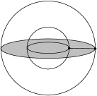
Figure 19. The cylinder over $S^{2}$

The computation is then straightforward:

$$\frac{1}{\mathcal{D}^{2}}\sum_{X\in\operatorname{Irr}(\mathcal{C})}d_{X}\leavevmode\hbox to153.17pt{\vbox to106.99pt{\text{[drawing]}}}\cdot\leavevmode\hbox to153.17pt{\vbox to106.99pt{\text{[drawing]}}}=\frac{1}{\mathcal{D}^{2}}\sum_{X\in\operatorname{Irr}(\mathcal{C})}\leavevmode\hbox to57.51pt{\vbox to69.65pt{\text{[drawing]}}}\cdot\leavevmode\hbox to57.51pt{\vbox to70.3pt{\text{[drawing]}}} \varphi \mathbf{1} \mathbf{1} X \varphi^{*} \mathbf{1} \mathbf{1} X^{*} X X^{*} \varphi \mathbf{1} \mathbf{1} X \varphi^{*} \mathbf{1} \mathbf{1} X^{*} X X^{*}$$

$$\quad=\frac{1}{\mathcal{D}^{2}}\sum_{X\in\operatorname{Irr}(\mathcal{C})}d^{2}_{X}=1.$$

The first equality follows from the normalization of the pairing. The other two equalities are obvious.

5. Proof of independence of polytope decomposition

In this section, we give proofs of Theorem 4.3, Theorem 4.4, i.e. prove that TV invariants are independent of the choice of polytope decomposition. The proof is based on Theorem 3.3, Theorem 3.4, which state that any two decompositions can be obtained from one another by a sequence of moves M1–M3 and their inverses.

First, we fix some notation. Unless otherwise stated, we denote simple objects in $\mathcal{C}$ by $X_{i},X_{j}\dots$ and arbitrary objects by $A,B,\dots$. We let $N_{1}^{i_{1}\dots i_{k}}=\dim(\langle X_{i_{1}},\dots,X_{i_{k}}\rangle)$.

We will now show that the TV state sum is invariant under M1–M3.

Invariance under M1

First we consider move M1. Note that by applying M2 and M3, we can transform an open book with any number of pages to one with only one page (see Figure 20).

$$\raisebox{-0.5pt}{\includegraphics[scale={0.7}]{figures/book0.eps}}\xrightarrow{\text{add edge to each page}}\raisebox{-0.5pt}{\includegraphics[scale={0.7}]{figures/book1.eps}}$$

$$\xrightarrow{\text{add faces between new edges}}\raisebox{-0.5pt}{\includegraphics[scale={0.7}]{figures/book2.eps}}\xrightarrow{\text{remove all pages but one}}\raisebox{-0.5pt}{\includegraphics[scale={0.7}]{figures/book3.eps}}$$

Figure 20. Decomposing an open book into a single page book

Thus, it suffices to prove invariance under M1 in this special case. Drawing the dual graph in the vicinity of the vertex, invariance under M1 is equivalent to the following equality:

$$\frac{1}{\mathcal{D}^{2}}\sum_{j,k\in\operatorname{Irr}(\mathcal{C})}d_{j}d_{k}\leavevmode\hbox to99.38pt{\vbox to49.72pt{\text{[drawing]}}}=\sum_{i\in\operatorname{Irr}(\mathcal{C})}d_{i}\leavevmode\hbox to99.38pt{\vbox to49.64pt{\text{[drawing]}}} \varphi \varphi^{*} \dots \dots V_{1} V_{n} V_{n} V_{1} X_{j} X_{k} \varphi \varphi^{*} \dots \dots V_{1} V_{n} V_{n} V_{1} X_{i} \varphi \varphi^{*} \dots \dots V_{1} V_{n} V_{n} V_{1} X_{j} X_{k} \varphi \varphi^{*} \dots \dots V_{1} V_{n} V_{n} V_{1} X_{i}$$

Note the normalizing factor $\frac{1}{\mathcal{D}^{2}}$ which comes from the fact that we are removing a vertex.

Using semisimplicity of $\mathcal{C}$, it is easy to see that it suffices to show this equality in the special case when $V=V_{1}\otimes\dots\otimes V_{n}$ is simple:

$$\frac{1}{\mathcal{D}^{2}}\sum_{j,k\in\operatorname{Irr}(\mathcal{C})}d_{j}d_{k}\leavevmode\hbox to76.32pt{\vbox to41.35pt{\text{[drawing]}}}=\sum_{i\in\operatorname{Irr}(\mathcal{C})}d_{i}\leavevmode\hbox to76.32pt{\vbox to41.27pt{\text{[drawing]}}} \varphi \varphi^{*} V V X_{j} X_{k} \varphi \varphi^{*} V V X_{i} \varphi \varphi^{*} V V X_{j} X_{k} \varphi \varphi^{*} V V X_{i}$$

By Lemma 1.1, the right-hand side is equal to $\operatorname{coev}_{V}\colon\mathbf{1}\to V\otimes V^{*}$. Since $\operatorname{Hom}(\mathbf{1},V\otimes V^{*})$ is one-dimensional, the left-hand side is also a multiple of $\operatorname{coev}_{V}$. Composing it with the evaluation morphism $\operatorname{ev}_{V}$, we get

$$\frac{1}{\mathcal{D}^{2}}\sum_{j,k}d_{j}d_{k}N_{1}^{Vjk}=\frac{1}{\mathcal{D}^{2}}\sum_{j,k}N_{k^{*}}^{Vj}d_{k}d_{j}$$

$$\quad=\frac{1}{\mathcal{D}^{2}}\sum_{j}\Bigl{(}\sum_{k}N_{k^{*}}^{Vj}d_{k}\Bigr{)}d_{j}=\frac{1}{\mathcal{D}^{2}}\sum_{j}(d_{V}d_{j})d_{j}=d_{V},$$

which proves that the left-hand side is equal to $\operatorname{coev}_{V}$.

Invariance under M2

The invariance under M2 is seen as follows. By definition, the edge being removed is incident to exactly two faces $c_{1},c_{2}$. Each face bounds the same two 3-cells $F_{1},F_{2}$. In Figure 21, we draw the dual graphs. In each of the summands we have two graphs corresponding to cells $F_{1},F_{2}$, separated by a dot. The equality follows immediately from the fact that if $\varphi_{\alpha},\varphi^{\alpha}$ and $\psi_{\beta},\psi^{\beta}$ are dual bases, then so are $\varphi_{\alpha}\underset{\scriptstyle X_{i}}{\bullet}\psi_{\beta}$, $\psi^{\beta}\underset{\scriptstyle X_{i}^{*}}{\bullet}\varphi^{\alpha}$ (cf. Corollary 1.2).

$$\sum_{i,\alpha,\beta}d_{i}\leavevmode\hbox to100.49pt{\vbox to49.64pt{\text{[drawing]}}}\leavevmode\hbox to100.49pt{\vbox to50.68pt{\text{[drawing]}}} \varphi_{\alpha} \psi_{\beta} \dots \dots V_{1} V_{n} W_{m} W_{1} X_{i} \varphi^{\alpha} \psi^{\beta} \dots \dots V_{n} V_{1} W_{1} W_{m} X^{*}_{i} \varphi_{\alpha} \psi_{\beta} \dots \dots V_{1} V_{n} W_{m} W_{1} X_{i} \varphi^{\alpha} \psi^{\beta} \dots \dots V_{n} V_{1} W_{1} W_{m} X^{*}_{i}$$

$$\quad=\sum_{i,\alpha,\beta}\leavevmode\hbox to74.66pt{\vbox to53.68pt{\text{[drawing]}}}\leavevmode\hbox to75.01pt{\vbox to53.65pt{\text{[drawing]}}} \varphi_{\alpha}\underset{\scriptstyle X_{i}}{\bullet}\psi_{\beta} V_{1} V_{n} W_{m} W_{1} \psi^{\beta}\underset{\scriptstyle X_{i}}{\bullet}\varphi^{\alpha} W_{1} W_{m} V_{m} V_{n} \varphi_{\alpha}\underset{\scriptstyle X_{i}}{\bullet}\psi_{\beta} V_{1} V_{n} W_{m} W_{1} \psi^{\beta}\underset{\scriptstyle X_{i}}{\bullet}\varphi^{\alpha} W_{1} W_{m} V_{m} V_{n}$$

Figure 21.

Invariance under M3

Finally, we consider M3. In this case the invaraince immediately follows from Lemma 1.3, whith two subgraphs corresponding to two 3-cells separated by the 2-cell being removed.

6. Surfaces with boundary

In this section we extend the definition of TV TQFT to surfaces with boundary (and 3-manifolds with corners). Recall that according to general ideas of extended field theory (see lurie), an extended 3d TQFT should assign to a closed 1-manifold a 2-vector space, or an abelian category, and to a 2-cobordism between two 1-manifolds, a functor between corresponding categories (which in the special case of cobordism between two empty 1-manifolds gives a functor $\mathcal{V}ec\to\mathcal{V}ec$, i.e. a vector space). In this section we show that the extension of the TV TQFT to 1-manifolds assigns to a circle $S^{1}$ the category $Z(\mathcal{C})$—the Drinfeld center of the original spherical category $\mathcal{C}$. This result was proved by Turaev in the special case when the original category $\mathcal{C}$ is ribbon (see turaev); the general case has remained a conjecture.

For technical reasons, it is more convenient to replace surfaces with boundaries by surfaces with embedded disks. These two notions give equivalent theories: given a surface with boundary, we can glue a disk to every boundary circle and get a surface with embedded disks; conversely, given a surface with embedded disks, one can remove the disks to get a surface with boundary. Moreover, in order to accommodate real-life examples, we need to consider framing. This leads to the following definition.

We denote

$$D^{2}=[0,1]\times[0,1]$$

and will call it the standard disk (it is, of course, a square, but this is what a disk looks like in PL setting). We will also the marked point $P_{0}$ on the boundary of $D^{2}$

$$P_{0}=(0,1)\in\partial D^{2}$$

Definition 6.1.

A framed embedded disk $D$ in a PL surface $N$ is the image of a PL map

$$\varphi\colon D^{2}\to N$$

which is a homeomorphism with the image, together with the point $P=\varphi(P_{0})\subset\partial D$.

An extended surface is a PL surface $N$ together with a finite collection of disjoint framed embedded disks (see Figure 22). We will denote the set of embedded disks by $D(N)$.

A coloring of an extended surface is a choice of an object $Y_{\alpha}\in\operatorname{Obj}Z(\mathcal{C})$ for every embedded disk $D_{\alpha}$.

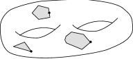
Figure 22. Extended surface

Next, we can define cobordisms between such surfaces. As usual, such a cobordism will be a 3-manifold with boundary together with some “tubes” inside which connect the embedded disks on the boundary of $M$. The following gives a precise definition in the PL category.

Definition 6.2.

Let $M$ be a PL 3-manifold with boundary.

An open embedded tube $T\subset M$ is the image of a PL map

$$\varphi\colon[0,1]\times D^{2}\to M$$

which is satisfies the conditions below, together with the oriented arc $\gamma=\varphi([0,1]\times\{P_{0}\})$ (which we will call the longitude).

The map $\varphi$ should satisfy:

1. $\varphi$ is a homeomorphism onto its image

2. $T\cap\partial M=\varphi(\{0\}\times D^{2})\cup\varphi(\{1\}\times D^{2})$

We will call the disks $B_{0}=\varphi(\{0\}\times D^{2})$ and $B_{1}=\varphi(\{1\}\times D^{2})$ the bottom and top disks of the tube.

A closed embedded tube $T\subset M$ is the image of a PL map

$$\varphi\colon S^{1}\times D^{2}\to M$$

which is satisfies the conditions below, together with the oriented arc $\gamma=\varphi([0,1]\times\{P_{0}\})$ (the longitude) and the disk $B=\varphi(\{0\}\times D^{2})\subset T$.

The map $\varphi$ should satisfy:

1. $\varphi$ is a homeomorphism onto its image

2. $T\cap\partial M=\varnothing$

The longitude $\gamma$ determines the framing of the tube; the disk $B$ is convenient for technical reasons; later we will get rid of it.

Definition 6.3.

An extended 3-manifold $M$ is an oriented PL 3-manifold with boundary together with a finite collection of disjoint framed tubes $T_{i}\subset M$. We denote the set of tubes of $M$ by $T(M)$.

A coloring of an extended 3-manifold $M$ is a choice of an object $Y_{\alpha}\in\operatorname{Obj}Z(\mathcal{C})$ for every tube $T_{\alpha}$.

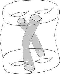
Figure 23. Extended 3-manifold

Note that if $M$ is an extended 3-manifold, then its boundary $\partial M$ has a natural structure of an extended surface: the embedded disks are the bottom and top disks of the open tubes, and the marked points on the boundary of embedded disks are the endpoints of the longitude arcs $\gamma_{\alpha}$, where $\alpha$ runs over the set of all open tubes in $M$. Moreover, a coloring of $M$ defines a coloring of $\partial M$: if an open tube $T_{\alpha}$ is colored with $Y_{\alpha}\in\operatorname{Obj}Z(\mathcal{C})$, we color the embedded disk $\varphi_{\alpha}(\{1\}\times D^{2})$ with $Y_{\alpha}$ and the embedded disk $\varphi_{\alpha}(\{0\}\times D^{2})$ with $Y_{\alpha}^{*}$.

Our main goal will be extending the TV invariants to such extended surfaces and cobordisms. Namely, we will

1. Define, for every colored extended surface $N$, the space $Z_{TV}(N,\{Y_{\alpha}\})$ which

   • functorially depends on colors $Y_{\alpha}$

   • is functorial under homeomorphisms of extended surfaces

   • has natural isomorphisms $Z_{TV}(\overline{N},\{Y_{\alpha}^{*}\})=Z_{TV}(N,\{Y_{\alpha}\})^{*}$

   • satisfies the gluing axiom for surfaces

2. Define, for every colored extended 3-manifold $M$, a vector $Z_{TV}(M)\in Z_{TV}(\partial M)$ (or, equivalently, for any colored extended 3-cobordism $M$ between colored extended surfaces $N_{1},N_{2}$, a linear map $Z_{TV}(M)\colon Z_{TV}(N_{1})\to Z_{TV}(N_{2})$) so that this satisfies the gluing axiom for extended 3-manifolds.

In the subsequent papers we will show that this extended theory actually coincides with the Reshetikhin–Turaev theory for the modular category $Z(\mathcal{C})$:

$$Z_{RT,Z(\mathcal{C})}=Z_{TV,\mathcal{C}}.$$

The construction of the theory proceeds similar to the construction of TV invariants. Namely, we will first define $Z_{TV}(N)$, $Z_{TV}(M)$ for manifolds with a polytope decomposition and then show that the so defined objects are independent of the choice of a polytope decomposition and thus define an invariant of extended manifolds.

7. Extended combinatorial surfaces

We begin by generalizing the definition of a polytope decomposition to extended surfaces.

Definition 7.1.

A combinatorial extended surface $\mathcal{N}$ is a an extended surface $N$ together with a polytope decomposition such that

1. The interior of each embedded disk is one of the 2-cells of the polytope decomposition.

2. Each marked point $P_{\alpha}$ on the boundary of an embedded disk is a vertex (0-cell) of the polytope decomposition.

We can now define the state space for such a surface. Let $\mathcal{N}$ be a combinatorial extended surface, and $Y_{\alpha},\alpha\in D(N)$, — a coloring of $\mathcal{N}$. Let $l$ be a labeling of edges of $\mathcal{N}$. Then we define the state space

$$H(\mathcal{N},\{Y_{\alpha}\},l)=\bigotimes_{C}H(C,l)$$

where the product is over all 2-cells of $\mathcal{N}$ (including the embedded disks) and

$$H(C,l)=\begin{cases}\langle Y_{\alpha},l(e_{1}),l(e_{2}),\dots,l(e_{n})\rangle&\quad C=D_{\alpha}\text{ -- an embedded disk}\\ \langle l(e_{1}),l(e_{2}),\dots,l(e_{n})\rangle&\quad C\text{ -- an ordinary 2-cell of $\mathcal{N}$}\end{cases}$$

where $e_{1},e_{2},\dots$ are edges of $C$ traveled counterclockwise; for the embedded disks, we also require that we start with the marked point $P_{\alpha}$; for ordinary 2-cells of $\mathcal{N}$ the choice of starting point is not important.

As usual, we now define

(7.1) $$H(\mathcal{N},\{Y_{\alpha}\})=\bigoplus_{l}H(\mathcal{N},\{Y_{\alpha}\},l)$$

where the sum is taken over all equivalence classes of simple labellings $l$ of edges of $\mathcal{N}$.

Note that so defined state space is functorial in $Y_{\alpha}$ and functorial under homeomorphism of extended surfaces; it is also immediate from the definition that one has a canonical isomorphism

$$H(\overline{\mathcal{N}},Y^{*}_{\alpha})=H(\mathcal{N},Y_{\alpha})^{*}.$$

Example 7.2.

Let $\mathcal{N}$ be the sphere with $n$ embedded disks and the cell decomposition shown in Figure 24.

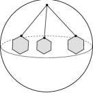
Figure 24. $n$-punctured sphere

Then

$$H(\mathcal{N},Y_{1},\dots,Y_{n})$$

$$\qquad=\bigoplus_{X_{1},\dots,X_{n},U_{1},\dots,U_{n}\in\operatorname{Irr}(\mathcal{C})}\langle X_{1},U_{1},X_{1}^{*},\dots,X_{n},U_{n},X_{n}^{*}\rangle\otimes\langle U_{1}^{*},Y_{1}\rangle\otimes\dots\otimes\langle U_{n}^{*},Y_{n}\rangle$$

$$\qquad\simeq\bigoplus_{X_{1},\dots,X_{n}\in\operatorname{Irr}(\mathcal{C})}\langle X_{1},Y_{1},X_{1}^{*},\dots,X_{n},Y_{n},X_{n}^{*}\rangle.$$

where the last isomorphism is given by direct sum of rescaled compositions (1.10).

The first main result of this paper is the gluing axiom for the so defined state space.

Theorem 7.3.

Let $\mathcal{N}$ be a combinatorial extended surface and $D_{a},D_{b}$ — two distinct embedded disks. Let $\mathcal{N}^{\prime}$ be the extended surface obtained by removing the disks $D_{a}$, $D_{b}$ and connecting the resulting boundary circles with a cylinder with the polytope decomposition consisting of a single 2-cell and a single 1-cell as shown below:

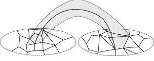
Figure 25. Gluing of extended surfaces. To help visualize the cylinder, it is colored light gray.

Thus, the set $D^{\prime}$ of embedded disks of $\mathcal{N}^{\prime}$ is $D^{\prime}=D(\mathcal{N})\setminus\{a,b\}$

Then one has a natural isomorphism

$$H(\mathcal{N}^{\prime},\{Y_{\alpha}\}_{\alpha\in D^{\prime}})=\bigoplus_{Z\in\operatorname{Irr}(Z(\mathcal{C}))}H(\mathcal{N},\{Y_{\alpha}\}_{\alpha\in D^{\prime}},Z,Z^{*})$$

where objects $Z,Z^{*}$ are assigned to embedded disks $D_{a},D_{b}$.

Proof.

For a given labeling $l$ of edges of $\mathcal{N}$, let

$$H_{0}(l)=\bigotimes_{C}H(C,l)$$

where the product is taken over all 2-cells of $\mathcal{N}$ (including the embedded disks) except $D_{a}$, $D_{b}$. Then

$$H(\mathcal{N},\{Y_{\alpha}\},Z,Z^{*},l)=H_{0}(l)\otimes\langle Z,A\rangle\otimes\langle Z^{*},B\rangle$$

where $A=l(e_{1})\otimes l(e_{2})\dots\otimes l(e_{n})$, where $e_{1},e_{2},\dots$ are edges of $D_{a}$ traveled counterclockwise starting with the marked point $P_{a}$, and similarly for $B$.

On the other hand, for a given labeling $l^{\prime}$ of edges of $\mathcal{N}^{\prime}$, we have

$$H(\mathcal{N}^{\prime},\{Y_{\alpha}\},l^{\prime})=H_{0}(l)\otimes\langle A\otimes l(e)\otimes B\otimes l(e)^{*}\rangle$$

where $l$ is the restriction of labeling $l^{\prime}$ to edges of $\mathcal{N}$, and $e$ is the added edge connecting marked points $P_{a}$, $P_{b}$.

Thus, the theorem immediately follows from the following lemma.

Lemma 7.4.

For any $A,B\in\operatorname{Obj}\mathcal{C}$, the map

(7.2) $$\bigoplus_{Z\in\operatorname{Irr}(Z(\mathcal{C}))}\langle Z,A\rangle\otimes\langle Z^{*},B\rangle \to\bigoplus_{X\in\operatorname{Irr}(\mathcal{C})}\langle A,X,B,X^{*}\rangle$$

$$\varphi\otimes\psi \mapsto\bigoplus_{X\in\operatorname{Irr}(\mathcal{C})}\frac{\sqrt{d_{X}}\sqrt{d_{Z}}}{\mathcal{D}}\quad\leavevmode\hbox to102.67pt{\vbox to62.6pt{\text{[drawing]}}} \varphi \psi A B Z X \varphi \psi A B Z X$$

is an an isomorphism.

(The factor $\sqrt{d_{X}}\sqrt{d_{Z}}/\mathcal{D}$ is introduced to make this isomorphism agree with pairing (1.6).)

Proof.

By Theorem 2.3, we have

$$\bigoplus_{X\in\operatorname{Irr}(\mathcal{C})}\langle A\otimes X\otimes B\otimes X^{*}\rangle=\bigoplus_{X}\operatorname{Hom}_{\mathcal{C}}(A^{*},X\otimes B\otimes X^{*})$$

$$\quad=\operatorname{Hom}_{\mathcal{C}}(A^{*},FI(B))=\operatorname{Hom}_{Z(\mathcal{C})}(I(A^{*}),I(B))$$

On the other hand,

$$\bigoplus_{Z\in\operatorname{Irr}(Z(\mathcal{C}))}\langle Z,A\rangle\otimes\langle Z^{*},B\rangle=\bigoplus_{Z}\operatorname{Hom}_{\mathcal{C}}(Z^{*},A)\otimes\operatorname{Hom}_{\mathcal{C}}(Z,B)$$

$$\quad=\bigoplus_{Z}\operatorname{Hom}_{Z(\mathcal{C})}(Z^{*},I(A))\otimes\operatorname{Hom}_{Z(\mathcal{C})}(Z,I(B))$$

$$\quad=\bigoplus_{Z}\operatorname{Hom}_{Z(\mathcal{C})}(I(A)^{*},Z)\otimes\operatorname{Hom}_{Z(\mathcal{C})}(Z,I(B))$$

$$\quad=\operatorname{Hom}_{Z(\mathcal{C})}(I(A)^{*},I(B))$$

(using semisimplicity of $Z(\mathcal{C})$). ∎

This completes the proof of the lemma and thus the theorem. ∎

8. Invariants of extended 3-manifolds

We begin by generalizing the definition of a polytope decomposition to extended 3-manifolds as defined in Definition 6.3.

Definition 8.1.

A combinatorial extended 3-manifold $\mathcal{M}$ is an extended PL 3-manifold with a polytope decomposition such that

• For an open tube $T_{\alpha}$, its interior is a single 3-cell of the decomposition. Moreover, the interior of the “bottom disk” $B_{0}=\varphi_{\alpha}(\{0\}\times D^{2})$ is a single 2-cell of the decomposition, and the marked point $P$ on the boundary of the bottom disk is a vertex of the decomposition, and similarly for the top disk $B_{1}=\varphi_{\alpha}(\{1\}\times D^{2})$.

• For a closed tube $T_{\alpha}$, the interior of the disk $B_{\alpha}=\varphi_{\alpha}(\{0\}\times D^{2})$ is a single 2-cell of the decomposition, the marked point $P_{\alpha}\in\partial B_{\alpha}$ is a vertex of the decomposition, and the complement $\operatorname{Int}(T_{\alpha})-B_{\alpha}$ is a single 3-cell of the decomposition.

Note that this implies that the restriction of such a polytope decomposition to the boundary of $\partial M$ satisfies the conditions of Definition 7.1 and thus defines on $\partial M$ the structure of a combinatorial extended surface. It also this implies that $\mathcal{M}$ contains two kinds of 3-cells: usual cells (which are not contained in any tube) and “tube cells”, i.e. cells contained in one of the tubes. The boundary of a usual 3-cell is a union of usual 2-cells; the boundary of a 3-cell corresponding to an open tube contains usual 2-cells and two embedded disks; the boundary of a 3-cell corresponding to a closed tube contains usual 2-cells and two copies of the disk $B_{\alpha}$ with opposite orientation.

Finally, note that we have imposed no restriction on the longitude of the tube: it is allowed (and usually will) intersect the edges of the decomposition of the boundary tubes.

The following theorem is an analog of Theorem 3.4.

Theorem 8.2.

Let $M$ be an extended 3-manifold. Then any two polytope decompositions $\mathcal{M}^{\prime},\mathcal{M}^{\prime\prime}$ of $\mathcal{M}$ which satisfy the conditions of Definition 8.1 and agree on $\partial M$ can be obtained from each other by a sequence of moves M1—M3 and their inverses such that all intermediate decompositions also satisfy the conditions of Definition 8.1 and agree with $\mathcal{M}^{\prime},\mathcal{M}^{\prime\prime}$ on $\partial M$.

Proof.

Let us consider the manifold $\tilde{M}$ obtained by removing from $M$ the interior of every tube and also the interior of the embedded disks on the boundary of $M$. Then $\tilde{M}$ is a manifold with boundary

$$\partial\tilde{M}=(\partial M-\cup\operatorname{Int}(D_{\alpha}))\cup\partial\tilde{M}_{free}$$

where the “free boundary” $\partial\tilde{M}_{free}$ is the union of side surfaces $I\times\partial D^{2}$ of the tubes (for closed tubes, $S^{1}\times\partial D^{2}$).

Obviously, polytope decompositions $\mathcal{M}^{\prime},\mathcal{M}^{\prime\prime}$ satisfying the conditions of the theorem determine decomposition of $\tilde{M}$ which agree on the subset $X=(\partial M-\cup\operatorname{Int}(D_{\alpha}))\subset\partial\tilde{M}$. Now the result follows from Theorem 3.7. ∎

Recall that for usual oriented 3-cell $F$ and a choice of edge labeling $l$, we have defined the vector $Z_{TV}(F,l)\in H(\partial F,l)$ defined by (4.4). We can now generalize it to tube cells. Namely, let $l$ be an edge coloring of an extended combinatorial 3-manifold $\mathcal{M}$ and let $T_{\alpha}\subset M$ be an open tube, with the longitude $\gamma_{\alpha}$ and color $Y_{\alpha}\in Z(\mathcal{C})$. Since $T$ is homeomorphic to $[0,1]\times D^{2}\simeq D^{3}$— a 3-ball, the boundary $\partial T$ is homeomorphic to $S^{2}$; thus, the polytope decomposition of $T$ defines a polytope decomposition of $S^{2}$.

Let $\Gamma$ be the dual graph of this cell decomposition. We can connect the marked points on the top and bottom disks to the vertex of the dual graph corresponding to these disks; together with the longitude $\gamma$, this gives an oriented arc on the surface of the sphere whose endpoints are two distinct vertices of $\Gamma$. For every 2-cell $C\in\partial F$ (including the embedded disks), choose a vector $v_{C}\in H(C,l)^{*}$. Thus, we get a graph $\hat{\Gamma}$ of the type considered in Section 2, i.e. colored graph $\Gamma$ on the surface of the sphere together with a colored framed arc inside as shown in Figure 26.

    

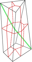
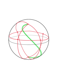
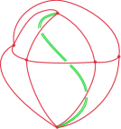
Figure 26. Dual graph for a tube cell. The longitude is shown by double green line.

By Theorem 2.4 this defines a number $Z_{RT}(\hat{\Gamma})$; as before, we let

(8.1) $$(Z(F,l),\otimes v_{C})=Z_{RT}(\hat{\Gamma}).$$

In a similar way we define the invariant for closed tubes.

We can now generalize the constructions of Section 4 to extended 3-manifolds.

Definition 8.3.

Let $\mathcal{M}$ be an extended combinatorial 3-manifold with boundary and $\mathcal{C}$ – a spherical category. Then for any edge coloring $l$ and a coloring $Y_{\alpha}$ of the tubes $T_{\alpha}\subset\mathcal{M}$, define the vector

$$Z_{TV}(\mathcal{M},\{Y_{\alpha}\},l)\in H(\partial\mathcal{M},\{Y_{\alpha}\},l)$$

by

$$Z_{TV}(\mathcal{M},l)=\operatorname{ev}\Bigl{(}\bigotimes_{F}Z(F,l)\Bigr{)}$$

where

• $F$ runs over all 3-cells in $M$ (including the tube cells), each taken with the induced orientation, so that

  $$\bigotimes_{F}Z(F,l)\in\bigotimes_{F}H(\partial F,l)=H(\partial\mathcal{M},l)\otimes\bigotimes_{c}H(c^{\prime},l)\otimes H(c^{\prime\prime},l)$$

  (compare with Lemma 3.2)

• $c$ runs over all unoriented 2-cells in the interior of $M$, including the disks $B_{\alpha}$ inside the closed tubes, and $c^{\prime},c^{\prime\prime}$ are the two orientations of such a cell, so that $c^{\prime}=\overline{c^{\prime\prime}}$.

• $\operatorname{ev}$ is the tensor product over all $c$ of evaluation maps $H(c^{\prime},l)\otimes H(c^{\prime\prime},l)=H(c^{\prime},l)\otimes H(c^{\prime},l)^{*}\to\mathbf{k}$

Finally, we define

(8.2) $$Z_{TV}(\mathcal{M},\{Y_{\alpha}\})=\mathcal{D}^{-2v(\mathcal{M})}\sum_{l}\Bigl{(}Z_{TV}(\mathcal{M},\{Y_{\alpha}\},l)\prod_{e}d^{n_{e}}_{l(e)}\Bigr{)}$$

where

• the sum is taken over all equivalence classes of simple labellings of $\mathcal{M}$,

• $e$ runs over the set of all (unoriented) edges of $\mathcal{M}$

• $\mathcal{D}$ is the dimension of the category $\mathcal{C}$ (see (1.1)), and

  $$v(\mathcal{M})=\text{number of internal vertices of }\mathcal{M}+\frac{1}{2}\text{(number of vertices on }\partial\mathcal{M})$$

• $d_{l(e)}$ is the categorical dimension of $l(e)$ and

  $$n_{e}=\begin{cases}1,&\quad e\text{ is an internal edge}\\ \tfrac{1}{2},&\quad e\in\partial\mathcal{M}\end{cases}$$

Note that in this definition, edges and vertices on the boundary of the tubes are considered internal unless they are also on $\partial\mathcal{M}$.

Theorem 8.4.

1. $Z_{TV}(\mathcal{M})$ satisfies the gluing axiom: if $\mathcal{M}$ is an extended combinatorial 3-manifold with boundary $\partial\mathcal{M}=\mathcal{N}_{0}\cup\mathcal{N}\cup\overline{\mathcal{N}}$, and $\mathcal{M}^{\prime}$ is the manifold obtained by identifying boundary components $\mathcal{N},\overline{\mathcal{N}}$ of $\partial\mathcal{M}$ with the obvious cell decomposition (if $\mathcal{N}$ contains embedded disks, then we may need to erase them so that the interior of resulting tubes have exactly one 3-cell), then we have

   $$Z_{TV}(\mathcal{M}^{\prime})=\operatorname{ev}_{H(\mathcal{N})}Z_{TV}(\mathcal{M})=\sum_{\alpha}(Z_{TV}(\mathcal{M}),\varphi_{\alpha}\otimes\varphi^{\alpha}),$$

   where $\operatorname{ev}$ is the evaluation map $H(\mathcal{N})\otimes H(\overline{\mathcal{N}})\to\mathbf{k}$, and $\varphi_{\alpha}\in H(\mathcal{N})$, $\varphi^{\alpha}\in H(\overline{\mathcal{N}})$ are dual bases.

2. If a $M$ is an extended PL 3-manifold, and $\mathcal{M}^{\prime},\mathcal{M}^{\prime\prime}$ are two polytope decompositions of $M$ which agree on the boundary, then $Z(\mathcal{M}^{\prime},\{Y_{\alpha}\})=Z(\mathcal{M}^{\prime\prime},\{Y_{\alpha}\})$.

3. For a combinatorial 2-manifold $\mathcal{N}$, define $A\colon H(\mathcal{N})\to H(\mathcal{N})$ by

   (8.3) $$A=Z_{TV}(\mathcal{N}\times I)$$

   Then $A$ is a projector: $A^{2}=A$.

4. For a combinatorial extended 2-manifold $\mathcal{N}$, define the vector space

   (8.4) $$Z_{TV}(\mathcal{N})=\mathrm{Im}(A\colon H(\mathcal{N})\to H(\mathcal{N}))$$

   where $A$ is the projector (8.3). Then the space $Z_{RT}(\mathcal{N})$ is an invariant of PL manifolds: if $\mathcal{N}^{\prime},\mathcal{N}^{\prime\prime}$ are two different polytope decompositions of the same extended PL manifold $N$, then one has a canonical isomorphism $Z(\mathcal{N}^{\prime})\simeq Z(\mathcal{N}^{\prime\prime})$.

Proof.

The proof is parallel to the proof of Theorem 4.4. The only new ingredient is in the proof of part (1), i.e. the gluing axiom for 3-manifolds: if the component of boundary along which we are gluing contains embedded disks, we need to erase them so that in the resulting manifold, interior of each tube is exactly one 3-cell. Thus, we need to check that our that $Z(\mathcal{M})$ is unchanged under this operation. The proof of this is similar to invariance under M3 move proved in Section 5. Details are left to the reader.

∎

Finally, we also note that our extended theory satisfies the gluing axiom for extended surfaces.

Theorem 8.5.

Under the assumptions of Theorem 7.3, one has a natural isomorphism

$$Z(\mathcal{N}^{\prime},\{Y_{\alpha}\}_{\alpha\in D^{\prime}})=\bigoplus_{Z\in\operatorname{Irr}(Z(\mathcal{C}))}Z(\mathcal{N},\{Y_{\alpha}\}_{\alpha\in D^{\prime}},Z,Z^{*})$$

where objects $Z,Z^{*}$ are assigned to embedded disks $a,b$.

Proof.

Recall that by Theorem 7.3, one has an isomorphism

$$G\colon\bigoplus_{Z\in\operatorname{Irr}(Z(\mathcal{C}))}H(\mathcal{N},\{Y_{\alpha}\}_{\alpha\in D^{\prime}},Z,Z^{*})\xrightarrow{\sim}H(\mathcal{N}^{\prime},\{Y_{\alpha}\}_{\alpha\in D^{\prime}})$$

Since $Z(\mathcal{N})$ is defined as the image of the projector $A\colon H(\mathcal{N})\to H(\mathcal{N})$, and similarly for $Z(\mathcal{N}^{\prime})$, it suffices to prove that the following diagram is commutative:

or equivalently, that for any $\varphi\in H(\mathcal{N},Z,Z^{*})$, $\varphi^{\prime}\in H(\overline{\mathcal{N}},Z,Z^{*})$, we have

$$(Z(\mathcal{N}\times I,Z,Z^{*}),\varphi\otimes\varphi^{\prime})=(Z(\mathcal{N}^{\prime}\times I),G(\varphi)\otimes G(\varphi^{\prime})).$$

Comparing both sides, we see that the only difference is that $\mathcal{N}\times I$ contains a pair of cylinders $D_{a}\times I,D_{b}\times I$:

whereas $\mathcal{N}^{\prime}\times I$ contains instead a single cell $C\times I$, where $C$ is the cylinder connecting boundary circles $\partial D_{a},\partial D_{b}$:

Thus, it suffices to prove that for any collection

$$\varphi_{a}\in H(D_{a})=\langle A,Z\rangle,\qquad \varphi_{b}\in H(D_{b})=\langle B,Z^{*}\rangle,$$

$$\varphi^{\prime}_{a}\in H(D_{a})^{*}=\langle(A^{\prime})^{*},Z^{*}\rangle,\qquad \varphi_{b}\in H(D_{b})^{*}=\langle(B^{\prime})^{*},Z\rangle,$$

$$\psi_{a}\in H(\partial D_{a}\times I)=\langle X_{k},A^{\prime},X_{k}^{*},A^{*}\rangle,\qquad \psi_{b}\in H(\partial D_{b}\times I)=\langle X_{l},B^{\prime},X_{l}^{*},B^{*}\rangle$$

we have

$$Z(D_{a}\times I,\varphi_{a}\otimes\varphi_{a}^{\prime}\otimes\psi_{a})\cdot Z(D_{b}\times I,\varphi_{b}\otimes\varphi_{b}^{\prime}\otimes\psi_{b})$$

$$\quad=\sum_{i,j}\sqrt{d_{i}}\sqrt{d_{j}}\ Z(C\times I,\psi_{a},\psi_{b},G(\varphi_{a}\otimes\varphi_{b}),G(\varphi^{\prime}_{a}\otimes\varphi^{\prime}_{b}))$$

(the factors $\sqrt{d_{i}}$, $\sqrt{d_{j}}$ appear because $\mathcal{N}^{\prime}\times I$ contains two extra edges on the boundary, labeled $i,j$.)

The left hand side is given by

$$LHS=\leavevmode\hbox to158.26pt{\vbox to109.54pt{\text{[drawing]}}}\cdot\qquad\leavevmode\hbox to158.26pt{\vbox to109.54pt{\text{[drawing]}}} \psi_{a} \varphi^{\prime}_{a} \varphi_{a} Z A^{\prime} A k \psi_{b} \varphi^{\prime}_{b} \varphi_{b} Z^{*} B^{\prime} B l$$

Combining explicit computation given in Section 9.1 with the formula for gluing in Lemma 7.4, we see that the right hand side is given by

$$RHS=\sum_{i,j}\frac{d_{i}d_{j}d_{Z}}{\mathcal{D}^{2}}\leavevmode\hbox to274.95pt{\vbox to150.08pt{\text{[drawing]}}} \psi_{a} \varphi \psi_{b} \varphi^{*} \varphi^{\prime}_{a} \varphi^{\prime}_{b} \varphi_{a} \varphi_{b} Z Z^{*} k l l A^{\prime} B^{\prime} i A B j k \psi_{a} \varphi \psi_{b} \varphi^{*} \varphi^{\prime}_{a} \varphi^{\prime}_{b} \varphi_{a} \varphi_{b} Z Z^{*} k l l A^{\prime} B^{\prime} i A B j k$$

Using Lemma 1.1, we can rewrite it as

$$RHS=\sum_{j}\frac{d_{j}d_{Z}}{\mathcal{D}^{2}}\leavevmode\hbox to243.62pt{\vbox to139.42pt{\text{[drawing]}}} \psi_{a} \psi_{b} \varphi^{\prime}_{a} \varphi^{\prime}_{b} \varphi_{a} \varphi_{b} A^{\prime} B^{\prime} j A B k l \psi_{a} \psi_{b} \varphi^{\prime}_{a} \varphi^{\prime}_{b} \varphi_{a} \varphi_{b} A^{\prime} B^{\prime} j A B k l$$

Since it follows from Lemma 2.2 that for any simple $Z\in\operatorname{Obj}Z(\mathcal{C})$ and a morphism $\Phi\in\operatorname{Hom}_{\mathcal{C}}(Z,Z)$, we have

$$\frac{1}{\mathcal{D}^{2}}\sum_{j}d_{j}\quad\leavevmode\hbox to51.4pt{\vbox to87.98pt{\text{[drawing]}}}=\frac{1}{d_{Z}}\operatorname{tr}(\Phi)\operatorname{id}_{Z} \Phi Z Z j \Phi Z Z j$$

this easily implies that the LHS is equal to RHS.

∎

Example 8.6.

Let $\mathcal{N}$ be the sphere with $n$ embedded disks, colored by objects $Y_{1},\dots,Y_{n}\in\operatorname{Obj}Z(\mathcal{C})$ (see Example 7.2). Then

$$Z(\mathcal{N},Y_{1},\dots,Y_{n})=\operatorname{Hom}_{Z(\mathcal{C})}(\mathbf{1},Y_{1}\otimes Y_{2}\otimes\dots\otimes Y_{n}).$$

Indeed, by Example 7.2, we have

$$H(\mathcal{N},Y_{1},\dots,Y_{n})=\bigoplus_{i_{1},\dots,i_{n}\in\operatorname{Irr}(\mathcal{C})}\langle X_{i_{1}},Y_{1},X_{i_{1}}^{*},\dots,X_{i_{n}},Y_{n},X_{i_{n}}^{*}\rangle.$$

By a direct computation done in Section 9, we see that the operator $A=Z(\mathcal{N}\times I)\colon H(\mathcal{N})\to H(\mathcal{N})$ is given by

$$\varphi\mapsto \frac{1}{\mathcal{D}^{2(n+1)}}\sum_{l,j_{1},\dots,j_{n}\in\operatorname{Irr}(\mathcal{C})}d_{l}\prod_{a=1}^{n}\sqrt{d_{i_{a}}}\sqrt{d_{j_{a}}}$$

Consider now the subspace $W\subset H(\mathcal{N},Y_{1},\dots,Y_{n})$ spanned by elements of the form

$$\bigoplus_{j_{1},\dots,j_{n}}\prod_{a=1}^{n}\sqrt{d_{j_{a}}}\quad\leavevmode\hbox to202.4pt{\vbox to79.87pt{\text{[drawing]}}} \psi Y_{1} Y_{n} j_{1} j_{n} \dots \psi Y_{1} Y_{n} j_{1} j_{n} \dots$$

$$\quad\psi\in\operatorname{Hom}_{Z(\mathcal{C})}(\mathbf{1},Y_{1}\otimes\dots\otimes Y_{n})$$

Clearly, $W\simeq\operatorname{Hom}_{Z(\mathcal{C})}(\mathbf{1},Y_{1}\otimes\dots\otimes Y_{n})$.

Now, it follows from the previous computation and Lemma 2.2 that for any $\varphi\in H(\mathcal{N},Y_{1},\dots,Y_{n})$, we have $A\varphi\in W$; on the other hand, it is immediate that if $\psi\in W$, then $A\psi=\psi$. Therefore, $A$ is the projector onto $W\simeq\operatorname{Hom}_{Z(\mathcal{C})}(\mathbf{1},Y_{1}\otimes\dots\otimes Y_{n})$.

9. Some computations

In this section we give some explicit computations of the TV invariants.

9.1. Cylinder over an annulus

Let $F=S^{1}\times I\times I$ be the cylinder over an annulus, as shown below.

Then

$$\partial F=C_{a}\cup C_{b}\cup C_{in}\cup C_{out}\cup C\cup\overline{C}$$

where $C_{a},C_{b}$ are the left and right annuli, $C_{in}$ and $C_{out}$ are the inner and outer cylinders, and $C$ is the internal cell:

$$C_{a}=\leavevmode\hbox to101.56pt{\vbox to87.07pt{\text{[drawing]}}}\qquad C_{b}=\leavevmode\hbox to102.15pt{\vbox to87.07pt{\text{[drawing]}}} A A^{\prime} k B B^{\prime} l A A^{\prime} k B B^{\prime} l$$

$$C_{in}=\leavevmode\hbox to72.2pt{\vbox to55.58pt{\text{[drawing]}}}\qquad C_{out}=\leavevmode\hbox to75.28pt{\vbox to59.46pt{\text{[drawing]}}}\qquad C=\leavevmode\hbox to65.31pt{\vbox to57.52pt{\text{[drawing]}}} A i B i A^{\prime} j B^{\prime} j k j l i A i B i A^{\prime} j B^{\prime} j k j l i$$

The pullback of the cell decomposition of $\partial F\simeq S^{2}$ to the sphere is homeomorphic to the cube shown below:

Drawing the dual graph, we see that given a collection

$$\psi_{L}\in H(\overline{C_{a}})=\langle A,X_{k},(A^{\prime})^{*},X_{k}^{*}\rangle,\qquad\psi_{R}\in H(\overline{C_{b}})=\langle B_{1}^{*},X_{l},B^{\prime},X_{l}^{*}\rangle$$

$$\psi_{in}\in H(\overline{C_{in}})=\langle A^{*},X_{i},B,X_{i}^{*}\rangle,\qquad\psi_{out}\in H(\overline{C_{out}})=\langle A^{\prime},X_{j},(B^{\prime})^{*},X_{j}^{*}\rangle$$

$$\varphi\in H(C)=\langle X_{l},X_{j}^{*},X_{k}^{*},X_{j}\rangle,\qquad\varphi^{\prime}\in H(\overline{C})=\langle X_{j}^{*},X_{k},X_{j},X_{l}^{*}\rangle,$$

the value $(Z(F),\psi_{L}\otimes\psi_{R}\otimes\psi_{in}\otimes\psi_{out}\otimes\varphi\otimes\varphi^{\prime})$ is given by the following graph:

9.2. Sphere with $n$ holes

Let $\mathcal{N}$ be the sphere with $n$ embedded disks, colored by objects $Y_{1},\dots,Y_{n}\in\operatorname{Obj}Z(\mathcal{C})$ (see Example 7.2). Choose the cell decomposition of $N$ as in Example 7.2; then

$$H(\mathcal{N},Y_{1},\dots,Y_{n})$$

$$\qquad=\bigoplus_{X_{1},\dots,X_{n},U_{1},\dots,U_{n}\in\operatorname{Irr}(\mathcal{C})}\langle X_{1},U_{1},X_{1}^{*},\dots,X_{n},U_{n},X_{n}^{*}\rangle\otimes\langle U_{1}^{*},Y_{1}\rangle\otimes\dots\otimes\langle U_{n}^{*},Y_{n}\rangle$$

$$\qquad\simeq\bigoplus_{X_{1},\dots,X_{n}\in\operatorname{Irr}(\mathcal{C})}\langle X_{1},Y_{1},X_{1}^{*},\dots,X_{n},Y_{n},X_{n}^{*}\rangle.$$

Consider now the cylinder $\mathcal{N}\times I$ with the cell decomposition shown in Figure 27.

Figure 27. Cylinder over sphere with $n$ embedded disks

This cell decomposition contains $(n+1)$ 3-cells: $n$ open tubes and one large 3-cell. Thus, the invariant $Z(\mathcal{N}\times I)$ is given by

$$(Z(\mathcal{N}\times I),\varphi\otimes\varphi^{\prime})=\sum_{l,k_{1},\dots,k_{n}\in\operatorname{Irr}(\mathcal{C})}D\cdot Z_{0}\cdot\dots\cdot Z_{n}$$

where

$$\varphi =\varphi_{0}\otimes\varphi_{1}\otimes\dots\otimes\varphi_{n}\in H(\mathcal{N},i_{1},\dots,i_{n})$$

$$\qquad=\langle X_{i_{1}},U_{1},X_{i_{1}}^{*},\dots,X_{i_{n}},U_{n},X_{i_{n}}^{*}\rangle\otimes\langle U_{1}^{*},Y_{1}\rangle\otimes\dots\otimes\langle U_{n}^{*},Y_{n}\rangle$$

$$\varphi^{\prime} =\varphi^{\prime}_{0}\otimes\varphi^{\prime}_{1}\otimes\dots\otimes\varphi^{\prime}_{n}\in H(\mathcal{N},j_{1},\dots,j_{n})^{*}$$

$$\qquad=\langle X_{j_{n}},V^{*}_{n},X_{j_{n}}^{*},\dots,X_{j_{1}},V^{*}_{1},X_{j_{1}}^{*}\rangle\otimes\langle V_{1},Y_{1}^{*}\rangle\otimes\dots\otimes\langle V_{n},Y_{n}^{*}\rangle$$

$D$ is the normalization factor:

$$D=\frac{1}{\mathcal{D}^{2(n+1)}}d_{l}\prod_{a=1}^{n}d_{k_{a}}\sqrt{d_{i_{a}}}\sqrt{d_{j_{a}}}\sqrt{d_{U_{a}}}\sqrt{d_{V_{a}}}$$

and $Z_{0},\dots,Z_{n}$ are the factors corresponding to the $(n+1)$ 3-cells of the decomposition:

$$Z_{0} =\quad\leavevmode\hbox to276.25pt{\vbox to137.07pt{\text{[drawing]}}} \varphi_{0} \varphi^{\prime}_{0} \alpha_{1} \beta_{1} \alpha_{1}^{*} \alpha_{n} \beta_{n} \alpha_{n}^{*} i_{1} j_{1} U_{1} V_{1} i_{1} j_{1} i_{n} j_{n} U_{n} V_{n} i_{n} j_{n} l l l \varphi_{0} \varphi^{\prime}_{0} \alpha_{1} \beta_{1} \alpha_{1}^{*} \alpha_{n} \beta_{n} \alpha_{n}^{*} i_{1} j_{1} U_{1} V_{1} i_{1} j_{1} i_{n} j_{n} U_{n} V_{n} i_{n} j_{n} l l l$$

$$Z_{i} =\quad\leavevmode\hbox to105.77pt{\vbox to124.06pt{\text{[drawing]}}} \varphi_{i} \beta_{i}^{*} \varphi^{\prime}_{i} U_{i} V_{i} Y_{i} k_{i} \varphi_{i} \beta_{i}^{*} \varphi^{\prime}_{i} U_{i} V_{i} Y_{i} k_{i}$$

Using Lemma 1.3, we see that it can be rewritten as follows:

$$(Z(\mathcal{N}\times I),\varphi\otimes\varphi^{\prime}) =$$

$$\sum_{l,k_{1},\dots,k_{n}\in\operatorname{Irr}(\mathcal{C})} D\qquad\leavevmode\hbox to276.25pt{\vbox to137.07pt{\text{[drawing]}}} \varphi_{0} \varphi^{\prime}_{0} \alpha_{1} \varphi_{1} \varphi^{\prime}_{1} \alpha_{1}^{*} \alpha_{n} \varphi_{n} \varphi^{\prime}_{n} \alpha_{n}^{*} i_{1} j_{1} U_{1} Y_{1} V_{1} i_{1} j_{1} i_{n} j_{n} U_{n} V_{n} Y_{1} i_{n} j_{n} k_{1} l l k_{n} l \varphi_{0} \varphi^{\prime}_{0} \alpha_{1} \varphi_{1} \varphi^{\prime}_{1} \alpha_{1}^{*} \alpha_{n} \varphi_{n} \varphi^{\prime}_{n} \alpha_{n}^{*} i_{1} j_{1} U_{1} Y_{1} V_{1} i_{1} j_{1} i_{n} j_{n} U_{n} V_{n} Y_{1} i_{n} j_{n} k_{1} l l k_{n} l$$

Thus, identifying $H(\mathcal{N},i_{1},\dots,i_{n})\simeq\langle X_{i_{1}},Y_{1},X_{i_{1}}^{*},\dots)$ as in Example 7.2 and using Lemma 1.1, we see that

$$(Z(\mathcal{N}\times I),\varphi\otimes\varphi^{\prime}) =\sum_{l\in\operatorname{Irr}(\mathcal{C})}\frac{1}{\mathcal{D}^{2(n+1)}}d_{l}\prod_{a=1}^{n}\sqrt{d_{i_{a}}}\sqrt{d_{j_{a}}}$$