Revisiting $\Delta Y/\Delta Z$ from multiple main sequences in Globular Clusters: insight from nearby stars

Abstract

For nearby K dwarfs, the broadening of the observed Main Sequence at low metallicities is much narrower than expected from isochrones with the standard helium–to–metal enrichment ratio $\Delta Y/\Delta Z\sim 2$. Though the latter value fits well the Main Sequence around solar metallicity, and agrees with independent measurements from HII regions as well as with theoretical stellar yields and chemical evolution models, a much higher $\Delta Y/\Delta Z\sim 10$ is necessary to reproduce the broadening observed for nearby subdwarfs. This result resembles, on a milder scale, the very high $\Delta Y/\Delta Z$ estimated from the multiple Main Sequences in $\omega$Cen and NGC 2808. Although not “inverted” as in $\omega$Cen, where the metal-rich Main Sequence is bluer than the metal-poor one, the broadening observed for nearby subdwarfs is much narrower than stellar models predict for a standard helium content. We use this empirical evidence to argue that a revision of lower Main Sequence stellar models, suggested from nearby stars, could significantly reduce the helium content inferred for the subpopulations of those globular clusters. A simple formula based on empirically calibrated homology relations is constructed, for an alternative estimate of $\Delta Y/\Delta Z$ in multiple main sequences. We find that, under the most favourable assumptions, the estimated helium content for the enriched populations could decrease from $Y\simeq 0.4$ to as low as $Y\simeq 0.3$.

1 Introduction

Helium is the second most abundant element in the Universe, having been produced by Big Bang Nucleosynthesis (BBN) with a universal mass fraction of $Y_{P}\sim$ 0.24 (Steigman 2007); after that, successive stellar generations synthesize metals ($Z$) and an additional amount of helium $\Delta Y$. The characteristic helium–to–metal enrichment rate $\Delta Y/\Delta Z$ is estimated to be around 2, both observationally from HII regions (e.g. Fukugita & Kawasaki 2006; Peimbert et al. 2007; Izotov, Thuan & Stasinska 2007) and theoretically, from models of stellar nucleosynthesis and chemical evolution of the Galactic disc (e.g. Chiosi & Matteucci 1982; Maeder 1992; Carigi & Peimbert 2008; Casagrande 2008)

In spite of its large abundance, helium is an elusive element. It can be measured directly, from spectroscopic lines, only in stars hotter than $\sim 10,000$ K: young, massive stars (or their surrounding HII regions) or blue Horizontal Branch stars (where though, apart from a small temperature range, the surface abundance may not trace the original one, due to helium sedimentation and metal levitation: Michaud, Vauclair & Vauclair 1983; Michaud, Richer & Richard 2008; Villanova, Piotto & Gratton 2009 and references therein). Only indirect methods can be used for stars of lower mass and cooler temperatures, which constitute the bulk of the Galaxy’s stellar population. One such method relies on the broadening of the lower Main Sequence (MS): in fact the location of low–mass, long–lived stars in the HR diagram depends on their metallicity $Z$ and their helium content $Y$ — or equivalently, on $\Delta Y/\Delta Z$. Concomitant increases in $Z$ and $Y$ shift the MS in opposite directions, so for a given variation $\Delta Z$ the two MSs are more spread apart (the metal rich being cooler at a given luminosity) if the corresponding $\Delta Y$ is lower; conversely, if $\Delta Y$ is large “enough”, the MSs may even invert, with the more metal (and helium) rich being bluer (i.e. hotter; e.g. Fernandes et al. 1996).

This method dates back to Faulkner (1967); early studies based on ground–based parallaxes deduced a large and quite uncertain value of $\Delta Y/\Delta Z\sim 5\pm 3$ from the apparent overlap of MSs of all metallicities (e.g. Perrin et al. 1977; Fernandes et al. 1996). The situation greatly improved with Hipparcos parallaxes, so that a net separation of the MS as a function of $Z$ could be detected in the HR diagram. Studies based on Hipparcos distances concluded $\Delta Y/\Delta Z=2-3$ (Pagel & Portinari 1998; Jimenez et al. 2003). More recently, Casagrande et al. (2006, 2007) further improved the analysis by compiling a much larger sample of K dwarfs with homogeneous multi–band photometry, for which bolometric magnitudes and effective temperatures were derived with the InfraRed Flux Method (IRFM). The interpretation of the broadening of the lower MS could thus be performed in the theoretical HR diagram ($M_{\rm{Bol}}$ vs. $\log T_{\rm{eff}}$) where comparison to stellar models is more straightforward and the effects of $\Delta Y/\Delta Z$ more prominent (Castellani, Degl’Innocenti & Marconi 1999). Around solar metallicities this analysis yielded $\Delta Y/\Delta Z\sim 2$; but at lower $Z$ Casagrande et al. (2007) found that the observed Main Sequence is narrower than expected from stellar models computed under the standard assumption $\Delta Y/\Delta Z\sim 2$, thus implying a very steep $\Delta Y/\Delta Z\sim 10$ (Fig. 5). This change in slope is at odds with Galactic chemical evolution models, that predict a ratio substantially constant with $Z$ (Carigi & Peimbert 2008; Casagrande 2008); a constant $\Delta Y/\Delta Z\sim 2$ is also found for both metal-rich (e.g. Peimbert 2003; Balser 2006) and metal-poor (e.g. Fukugita & Kawasaki 2006; Peimbert et al. 2007; Izotoz et al. 2007) HII regions. More importantly, $\Delta Y/\Delta Z\sim 10$ at low metallicities implies a helium content for nearby subdwarfs much lower than $Y_{P}$, in awkward constrast with the cosmological floor set by standard BBN.

A combination of small sample size and $Z$–dependent bolometric corrections in the observational HR diagram had masked this effect in previous studies of $\Delta Y/\Delta Z$, although very low $Y$ values had already been noticed in a handful of low metallicity stars with available IRFM $M_{\rm{bol}}$ and $T_{\rm{eff}}$ (Fernandes et al. 1998; Lebreton et al. 1999). This result points toward inadequacies in Main Sequence stellar models of low metallicity, and we now plan to investigate the issue further, as this may lead to reconsideration of the problem of the helium enrichment in globular clusters.

In fact, at absolute magnitudes comparable to those of the local stars studied in Casagrande et al. (2007, $M_{V}\sim 5.5-7.5$), multiple Main Sequences have been discovered in some globular clusters and interpreted as evidence for huge helium enhancement in a sub-population (Bedin et al. 2004; Norris 2004; Piotto et al. 2005, 2007); see Fig. 1. The required $\Delta Y/\Delta Z\gtrsim 100$ is extremely difficult to explain with stellar nucleosynthesis and chemical evolution models (Karakas et al. 2006; Prantzos & Charbonnel 2006; Maeder & Meynet 2006; Choi & Yi 2007, 2008; Romano et al. 2007, 2009; Renzini 2008; Yi 2009; Marcolini et al. 2009; Peng & Nagai 2009).

The helium content of the sub-population also has a major role in shaping other regions of the HR diagram (Catelan, Valcarce & Sweigart 2009a and references therein); in particular it is reflected in the morphology of the Horizontal Branch (D’Antona & Caloi 2004; Caloi & D’Antona 2005, 2007; Lee et al. 2005). While it is likely that a significant helium enhancement is present in those stellar populations, the purpose of this work is to show that the revision of low metallicity MS stellar models, needed to cure the problem of the high $\Delta Y/\Delta Z$ and sub-primordial $Y$ deduced in nearby K dwarfs, may significantly reduce current estimates of $\Delta Y/\Delta Z$ in globular clusters with multiple MSs, easing their theoretical interpretation.

We show this by means of an exercise based on homology relations. Theoretical homology relations, describing how the location of the low MS in the HR diagram depends on metallicity and helium content, are briefly recalled in Section 2. In Section 3, we apply homology relations to interpret the split of multiple MSs in globular clusters, and show that the inferred helium enrichment for the blue population(s) agrees with the results of detailed isochrone analysis. In Section 4 we confirm that, in general, homology relations render very well the behaviour of stellar models as a function of the helium content. However, both isochrones and homology relations fail the interpretation of the low MS of nearby stars — as we cannot accept sub–primordial helium contents for low metallicity stars. Therefore, in Section 5 we proceed to calibrate empirical homology relations, that return the expected $\Delta Y/\Delta Z=2$ for the low MS of nearby stars with $Z<Z_{\odot}$. Such empirically calibrated homology relations also return, for the helium–rich subpopulations of globular clusters, a helium content $Y\sim 0.3$, rather than the much higher $Y\sim 0.35-0.4$ of standard analysis. This lower value of helium enrichment can be reconciled far more easily with present chemical evolution models (Karakas et al. 2006; Renzini 2008; Yi 2009). Finally, we conclude in Section 6 with a discussion of the possible physical processes that could improve stellar models for low MS stars, so as to solve the “helium problem” both for nearby stars and for globular clusters.

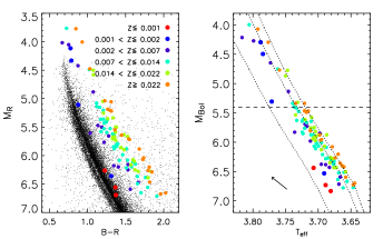
Figure 1: Left panel: HR diagram of nearby K dwarfs (filled circles) from the sample of Casagrande et al. (2007), overplotted on the MSs photometry of $\omega$Cen (Sollima et al. 2007), adopting $E(B-V)=0.11$ (Lub 2002) and dereddened distance modulus of 13.7 (Bellazzini et al. 2004; Del Principe et al. 2006). The maximum split between the red and blue MS of $\omega$Cen $\Delta(B-R)=0.1$ occurs around $M_{R}\sim M_{\rm{Bol}}\sim 6.5$ (Sollima et al. 2007). Right panel: nearby K dwarfs in the theoretical plane with isochrones having $Z=0.001,Z_{\odot},0.04$ and $\Delta Y/\Delta Z=2$ overplotted. Clear mismatch in the broadening appears for low metallicities. Below $M_{\rm{Bol}}=5.4$ the broadening of the MS is age independent. We also show the reddening/extinction correction corresponding to $E(B-V)=0.10$ that would be needed to reconcile the metal-poor stars with theoretical isochrones.

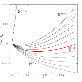
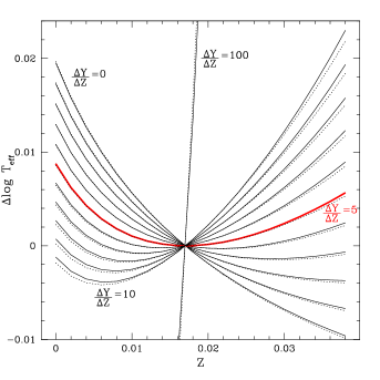
Figure 2: Broadening of the ZAMS in log $T_{\rm{eff}}$ as a function of metallicity, as predicted by homology relations (Eq. 2). The broadening is referred to the primordial ZAMS ($Z_{P}$, $Y_{P}$; left panel) or to the solar ZAMS ($Z_{\odot}=0.017$, $Y_{\odot}=0.263$; right panel) for $\frac{\Delta Y}{\Delta Z}$ ranging from 0 to 10 as indicated. Dotted lines show the approximate relation proposed in Eq. 3. The thick red line highlights the case $\frac{\Delta Y}{\Delta Z}=5$, which corresponds to MS inversion around $Z_{\odot}$. At increasing $\Delta Y/\Delta Z$, MS inversion occurs at lower and lower $Z$.

2 Homology relations

Homology relations (Cox & Giuli 1968), holding for radiative structures like the energy-producing cores of MS stars of $M$$\;\stackrel{{\scriptstyle\textstyle<}}{{\sim}}\;$1 $M_{\odot}$, express the difference in $M_{\rm{Bol}}$ of a Zero Age Main Sequence of composition ($Y,Z$) with respect to another reference ZAMS of composition ($Y_{r},Z_{r}$). In the hypothesis that the compositions are related by:

$$Y=Y_{r}+\frac{\Delta Y}{\Delta Z}(Z-Z_{r})$$

the formula is:

$$\begin{array}[]{l l}\Delta M_{\rm{Bol}}=\par\vskip 6.0pt plus 2.0pt minus 2.0pt&-1.59\log\left[1-\frac{\delta}{X_{r}}(Z-Z_{r})\right]\\ \vskip 6.0pt plus 2.0pt minus 2.0pt&-3.33\log\left[1-\frac{5\delta+1}{(3+5X_{r}-Z_{r})}(Z-Z_{r})\right]\\ \vskip 6.0pt plus 2.0pt minus 2.0pt&-0.8675\log\left[1-\frac{\delta}{(1+X_{r})}(Z-Z_{r})\right]\\ &-0.8675\log\left(\frac{100Z+1}{100Z_{r}+1}\right)\\ \end{array}$$ (1)

where $\delta=1+\frac{\Delta Y}{\Delta Z}$ and $X_{r}=1-Y_{r}-Z_{r}$. Notice that the same relation holds also for a generic combination of $(Y,Z)$ replacing $\delta\,(Z-Z_{r})\rightarrow(Y-Y_{r})+(Z-Z_{r})$. The first term is related to the rate of thermonuclear energy generation, the second term to the molecular weight, and the final two terms to opacity (Cox & Giuli 1968; Fernandes et al. 1996; see also the Appendix). For $Z_{r}=0$, $Y_{r}=Y_{P}$ (primordial helium floor due to BBN) this formula corresponds to eq. 3 of Pagel & Portinari (1998). Another typical approach is to refer to the solar ZAMS, as the solar model is the basic calibration of stellar tracks and isochrones; then ($Y_{r},Z_{r}$)=($Y_{\odot},Z_{\odot}$).

In the case of old stellar populations, because evolution affects luminosities approximately brighter than $M_{\rm{Bol}}$=5.4, it is more useful to translate the broadening in $M_{\rm{Bol}}$ into a broadening in $T_{\rm{eff}}$ using the slope of the lower MS. In the Padova isochrones used in Casagrande et al. (2007), this slope is about 17 mag per dex in log($T_{\rm{eff}}$), henceforth:

$$\begin{array}[]{l l}\Delta\log T_{\rm{eff}}=\par\vskip 6.0pt plus 2.0pt minus 2.0pt&-0.0935\log\left[1-\frac{\delta}{X_{r}}(Z-Z_{r})\right]\\ \vskip 6.0pt plus 2.0pt minus 2.0pt&-0.196\log\left[1-\frac{5\delta+1}{(3+5X_{r}-Z_{r})}(Z-Z_{r})\right]\\ \vskip 6.0pt plus 2.0pt minus 2.0pt&-0.051\log\left[1-\frac{\delta}{(1+X_{r})}(Z-Z_{r})\right]\\ &-0.051\log\left(\frac{100Z+1}{100Z_{r}+1}\right)\\ \end{array}$$ (2)

(cf. eq. 4 of Pagel & Portinari, with slightly different coefficients due to the different adopted slope of the MS). Fig. 2 shows the broadening of the MS as a function of metallicity, as predicted by homology relations. For low $\Delta Y/\Delta Z$ (e.g. $\Delta Y/\Delta Z=0$) the MS is cooler at increasing metallicity, as “normally” expected. When $\Delta Y/\Delta Z=5$, MS inversion is expected around solar metallicity (i.e. overlapping MS, as was deduced from pre–Hipparcos data). At increasing $\Delta Y/\Delta Z$, MS inversion — namely, more metal-rich MS being hotter due to the overwhelming effect of the helium excess $\Delta Y$ — occurs at lower and lower $Z$. Indeed, extremely high $\Delta Y/\Delta Z$ are necessary to interpret the MS inversion at the low $Z$ of $\omega$ Centauri.

3 Homology relations and globular clusters

Evidence for multiple stellar populations in some Globular Clusters comes from turn-off, subgiant and red giant branch splits; bi- or multi-modal distribution of light elements; and the presence of multiple, distinct MSs (e.g. Piotto 2009). In the latter case, because of the faintness of the stars, deep photometric observations are needed and clear evidence for multiple MSs is currently limited to $\omega$Cen and NGC 2808; in addition, evidence for MS broadening has been recently found in 47 Tuc (Anderson et al. 2009).

In this section we analyze the multiple MSs of the above mentioned clusters by means of homology relations, and compare the results to those obtained with modern isochrone fitting.

3.1 $\omega$ Cen

Detailed isochrone analysis indicates that a helium enrichment of $\Delta Y\simeq 0.15$ between the two populations is needed to reproduce the inverted MSs of $\omega$Cen (Norris 2004; Piotto et al. 2005; Lee et al. 2005; Sollima et al. 2007). We show here that homology relations yield a very similar result. To apply homology relations (Eq. 2), we must translate into a split in log $T_{\rm{eff}}$ the maximum observed colour split between the blue (bMS) and red (rMS) main sequence: $\Delta(B-R)=0.1$, which occurs at a dereddened $B-R=1.2$ for the rMS (Sollima et al. 2007). We apply the colour–temperature–metallicity scale of Casagrande et al. (2006) that was derived for nearby K dwarfs, adopting $\rm{[Fe/H]}_{\rm{rMS}}=-1.6$ and $\rm{[Fe/H]}_{\rm{bMS}}=-1.3$ (Sollima et al. 2007). We obtain for the rMS $T_{\rm{eff}}$=5120 K and $\Delta\log T_{\rm{eff}}=0.0185$ between the two sequences. Considering possible uncertainties in the reddening which affect the absolute $B-R$ values (while the differential $\Delta(B-R)=0.1$ is robust) we estimate $\Delta\log(T_{\rm{eff}})=0.0185\pm 0.0015$. Adopting the updated and extended temperature scale by Casagrande et al. (2010) also yields $\Delta\log T_{\rm{eff}}$ estimates within this range.

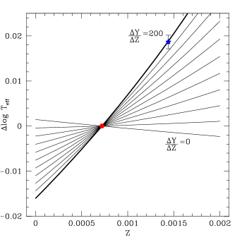
Figure 3: Temperature split of the MS predicted by homology relations compared to the split between the rMS (dot, taken as reference MS in Eq. 2) and the bMS (star symbol) of $\omega$Cen. The observed temperature split is $\Delta\log(T_{\rm{eff}})=0.0185\pm 0.0015$, and the assumed metallicities are $Z_{\rm{rMS}}=0.00072$ and $Z_{\rm{bMS}}=0.00144$ (see text). Lines indicate homology predictions for $\Delta Y/\Delta Z$ increasing from 0 to 200 in steps of 20. The observed split between the rMS and bMS is reproduced for $\Delta Y/\Delta Z\simeq 200$, corresponding to $\Delta Y=0.144$ and $Y_{\rm{bMS}}=0.39$.

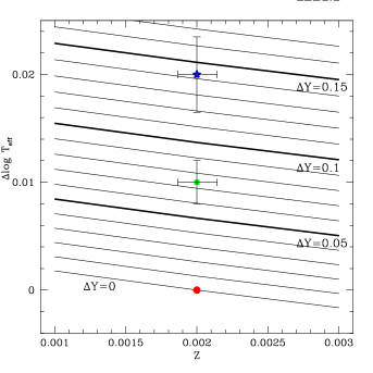
Figure 4: Temperature split of the MS predicted by homology relations compared to the split between the red MS (dot, taken as reference MS in Eq. 2), the middle MS (square symbol) and the blue MS (star symbol) of NGC 2808. In this figure homology relations are marked as a function of $\Delta Y$ rather than $\Delta Y/\Delta Z$ (see text), with $\Delta Y$ increasing from 0 to 0.17 in steps of 0.01. The observed splits are reproduced for $\Delta Y$(mMS-rMS)=0.074 and $\Delta Y$(bMS-rMS)=0.143, corresponding to $Y_{\rm{mMS}}=0.322$ and $Y_{\rm{bMS}}=0.391$. Errors bars are estimated converting in $\Delta\log T_{\rm{eff}}$ an uncertainty of 0.02 magnitudes for the value of $\Delta(B-I)$.

To derive the metal mass fraction $Z$ that is relevant for homology relations, we adopt for both sequences an enrichment $\rm{[\alpha/Fe]}=+0.3$ as supported by various spectroscopic studies (Sollima et al. 2007 and references therein; Villanova et al. 2007). Using the relation of Yi et al. (2001) to compute the global metallicity leads to $\rm{[M/H]}_{\rm{rMS}}=-1.37$ and $\rm{[M/H]}_{\rm{bMS}}=-1.07$. Simple scaling with $Z_{\odot}$ returns $Z_{\rm{rMS}}=0.00072$ and $Z_{\rm{bMS}}=0.00144$. We further assume $Y_{\rm{rMS}}=0.246$ — but note that the resulting $\Delta Y=Y_{\rm{bMS}}-Y_{\rm{rMS}}$ is not sensitive to the adopted value of $Y_{\rm{rMS}}$. Fig. 3 shows the split in $\Delta\log T_{\rm{eff}}$ predicted by homology relations with respect to the rMS, i.e. applying Eq. 2 with ($Y_{r}$,$Z_{r}$)=($Y_{\rm{rMS}},Z_{\rm{rMS}}$). The observed split between the rMS and bMS is reproduced for $\Delta Y/\Delta Z\simeq 200$, implying $\Delta Y=0.144$ and $Y_{\rm{bMS}}=0.39$. These values for $\Delta Y$ and $Y_{\rm{bMS}}$ are in excellent agreement with the results obtained by Piotto et al. (2005), Lee et al. (2005) and Sollima et al. (2007) by means of detailed isochrone analysis — while the value for $\Delta Y/\Delta Z$ may vary significantly, depending on the assumed difference in metallicity $\Delta Z$ in various studies. For instance, by adopting $Z_{\rm{rMS}}=0.001$ and $Z_{\rm{bMS}}=0.002$ as in Piotto et al. (2005), homology relations reproduce the observed temperature split with $\Delta Y/\Delta Z\simeq 150$, implying again $\Delta Y\simeq 0.15$ as a robust result. A rigorous transformation from $\rm{[M/H]}$ to $Z$ (e.g. Casagrande et al. 2007) should take into account also the very different helium fraction in the two sequences ($Y_{\rm{rMS}}=0.246$ and $Y_{\rm{bMS}}=0.39$), returning $Z_{\rm{rMS}}=0.00076$ and $Z_{\rm{bMS}}=0.00120$; homology relations then yield $\Delta Y/\Delta Z\simeq 320$, corresponding to $\Delta Y=0.14$. Thus, $\Delta Y=Y_{\rm{bMS}}-Y_{\rm{rMS}}$ is a robust result of the analysis.

It is worth underlining that, in any case, in $\omega$Cen $\Delta Y/\Delta Z>>70$, this value being correctly indicated by Piotto et al. (2005) as a lower limit, but often quoted in the literature as the preferred $\Delta Y/\Delta Z$. Values of $\Delta Y/\Delta Z\sim 200$ or higher are implied by the current metallicity measurements of the rMS and bMS (as also in Sollima et al. 2007), which renders the theoretical interpretation even more troublesome (see e.g. Yi 2009).

3.2 NGC 2808

Another striking example of helium enriched multiple Main Sequences is NGC 2808, where three MSs are found at virtually the same metallicity $\rm{[Fe/H]}=-1.1\pm 0.03$ dex (Carretta et al. 2006; see also Salaris et al. 2006) and helium abundances of $Y=0.248$ (the value assumed for the red MS, which includes the bulk of the population), $Y=0.30$ (middle MS) and $Y=0.37$ (blue MS; D’Antona et al. 2005; Lee et al. 2005; Piotto et al. 2007). In this case, formally $\Delta Y/\Delta Z\rightarrow\infty$ (or, $\Delta Y/\Delta Z>800$) and one should just focus on $\Delta Y$. Also in this case, we show that homology relations yield an estimate of $\Delta Y$ in good agreement with isochrone analysis.

As for wCen, the scale of Casagrande et al. (2006) was used to convert the colour split into a temperature split. In NGC2808, the maximum split of the bMS and rMS with respect to the mMS ($\pm 0.08$ mag) occurs around a magnitude $m_{\rm{F814W}}=21.3$, where the colour of the mMS is $\rm{F475W}-\rm{F814W}=1.72$. Correcting for reddening (E(B-V)=0.18, Piotto et al. 2007) and transforming the WFC/ACS Vegamag system photometry into Johnson–Cousins according to Sirianni et al. (2005), these colours and broadening correspond to $B-I=1.74$ and $\Delta(B-I)\pm 0.11$ mag, equivalent to $T_{eff}=5020$ K for the mid MS and $\Delta\log T_{\rm{eff}}=\pm 0.01$.

As $\Delta Z$ vanishes and $\Delta Y/\Delta Z$ diverges in the case of NGC 2808, it is convenient to recast the homology relation in Eq. 2 replacing $\delta\,(Z-Z_{r})\rightarrow(Y-Y_{r})+(Z-Z_{r})$. Fig. 4 compares the predicted temperature split as a function of $\Delta Y$ to the observed one. For an assumed $Y_{\rm{rMS}}=0.248$, the resulting $Y_{\rm{mMS}}=0.32$ and $Y_{\rm{bMS}}=0.39$ are again in excellent agreement with isochrone analysis (see Fig. 2 of Piotto et al. 2007).

3.3 47 Tuc

Theoretical homology relations agree very closely with detailed isochrone analysis in the estimate of the $\Delta Y$ and $\Delta Y/\Delta Z$, characterizing the split of the multiple MSs of $\omega$Cen and NGC 2808. We have checked that this holds true also for the (less extreme) case of 47 Tuc. The observed broadening of the MS of 47 Tuc is $\Delta(F606W-F814W)=0.013$ around an average colour $F606W-F814W\simeq 0.9$ at $F606W=20.5$; if interpreted in terms of a dispersion in helium abundance, this implies $\Delta Y=0.026$ (Anderson et al. 2009). To analyze the same dispersion with homology relations, we have translated the observed broadening into Johnson colours, and then into effective temperatures.

With the reddening and distance modulus listed in the catalogue by Harris (1996; in its 2003 online version) the broadening amounts to $\Delta(V-I)=0.017$ around $M_{V}=7.3$ and $V-I=1.04$. With a metallicity $\rm{[Fe/H]}=-0.76$ (Harris 2003; Carretta et al. 2009), this average $V-I$ colour corresponds to $T_{\rm{eff}}\sim 4800$ K and the broadening to $\Delta\log T_{\rm{eff}}=0.003$. Homology relations (Eq. 2) reproduce such broadening with $\Delta Y=0.023$, again very close to the conclusions from isochrone fitting.

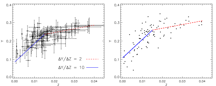
Figure 5: Metal versus helium mass fraction for nearby field dwarfs. Lines with two values of helium–to–metal enrichment ratio (break at $Z=0.015$) are plotted to guide the eye. Left panel: using the isochrone fitting procedure described in Casagrande et al. (2007). Right panel: using numerical homology relations (see Section 4).

4 Homology relations and isochrones

We have shown that theoretical homology relations, applied to the multiple (or broadened) MSs of globular clusters, provide a similar interpretation of the data in terms of $\Delta Y$ and $\Delta Y/\Delta Z$, as detailed isochrone analysis. We now compare directly homology relations to current stellar models. We fit the Padova isochrones as a function of $Z$ and $\Delta Y/\Delta Z$ with a homology–like relation and compare the fitted relation to the theoretical one.

An interpolation formula for isochrones directly inspired by Eq. 2 involves at least 4 independent parameters: the coefficients of the first 3 terms in Eq. 2, and the coefficient of $Z$ within the argument of the logarithm in the $4^{th}$ term. For fitting purposes, however, we found that a simplified form of the homology relations is more convenient. We derive it by condensing together the first three terms in Eq. 2, containing the dependence of the broadening on $\Delta Y/\Delta Z$. First of all we notice that those three terms have a similar dependence:

$$\propto\log\left[1-\frac{\delta}{(a+X_{r})}(Z-Z_{r})\right]\leavevmode\nobreak\ \leavevmode\nobreak\ \leavevmode\nobreak\ \leavevmode\nobreak\ \leavevmode\nobreak\ \leavevmode\nobreak\ \leavevmode\nobreak\ \leavevmode\nobreak\ \leavevmode\nobreak\ \leavevmode\nobreak\ \leavevmode\nobreak\ \leavevmode\nobreak\ \leavevmode\nobreak\ \leavevmode\nobreak\ \leavevmode\nobreak\ a=0,\leavevmode\nobreak\ 0.6\leavevmode\nobreak\ {\rm or}\leavevmode\nobreak\ 1$$

as in the second term we can approximate:

$$\frac{5\delta+1}{(3+5X_{r}-Z_{r})}(Z-Z_{r})\simeq\frac{5\delta}{(3+5X_{r})}(Z-Z_{r})$$

Secondly, it is easy to verify that the second term of Eq. 2 is the leading one, contributing about as much as the sum of the first and third term together. Guided by these considerations, we find that the following formula:

$$\begin{array}[]{l l}\vskip 6.0pt plus 2.0pt minus 2.0pt\Delta\log T_{\rm{eff}}=&-0.414\log\left[1-\frac{\delta}{(0.6+X_{r})}(Z-Z_{r})\right]\\ &-0.051\log\left(\frac{100Z+1}{100Z_{r}+1}\right)\\ \end{array}$$ (3)

is a very good approximation of the rigorous homology relations, especially for metallicities $Z\leq Z_{\odot}$ which are of interest for our discussion (Fig. 2). We have also verified that this is a fully adequate approximation of the full homology relations even for extremely high $\Delta Y/\Delta Z>100$, which are of interest for globular clusters, at least within narrow metallicity ranges (like those separating the sub-populations of e.g. $\omega$Cen). This simplified formulation has the advantage of separating one term sensitive to the helium content, from the second term which depends only on metallicity. This clearcut separation will prove to be handy for the empirical re-calibration of homology relations in Section 5.

Therefore we seek a three–parameter fitting formula for isochrones (and, later below, for real stars) of the kind:

$$\begin{array}[]{l l}\vskip 6.0pt plus 2.0pt minus 2.0pt\Delta\log T_{\rm{eff}}=&-P_{1}\log\left[1-\frac{\delta}{(0.6+X_{r})}(Z-Z_{r})\right]\\ &-P_{2}\log\left(\frac{P_{3}Z+1}{P_{3}Z_{r}+1}\right)\\ \end{array}$$ (4)

where $P_{i}$ are 3 free fitting parameters. It is our experience that this 3-parameter formula provides an adequate fit to isochrones, as good as (and more robust than) other homology-like fitting formulæ with 4 or more parameters. We favour this form of the homology relation over the linearized one adopted by Pagel & Portinari (1998; their eq. 5) as it is better suited to handle large values of $\Delta Y/\Delta Z$ (see the Appendix).

We consider both the Padova isochrones computed specifically for the analysis in Casagrande et al. (2007), and the more recent release by Bertelli et al. (2008) with varying $\Delta Y/\Delta Z$ and $0.0001\leq Z\leq 0.04$, which fully brackets the metallicity range relevant for the present study. In Casagrande et al. (2007) we had checked that other sets of isochrones (Yonsei–Yale, Teramo, McDonald) were very similar in the low MS.

We tried the fit both with respect to the solar ($Z_{\odot}=0.017$) and to a very metal-poor reference isochrone ($Z=0.0002$). We explored values of $\Delta Y/\Delta Z$ up to 1000, obtained both with sub-solar and sub-primordial helium contents (isochrones from Casagrande et al. 2007) and with helium–enhanced isochrones (Bertelli et al. 2008). Very similar parameters are obtained in both cases, as one would expect from the discussion in Section 2.

We find that the behaviour of isochrones, at least in the range $M_{\rm{Bol}}=5.4-7.0$ which is where the effect of $\Delta Y/\Delta Z$ is expected to be maximal and dominant, is well described by homology–like relations with the following set of parameters:

$$P_{1}=0.50\pm 0.03$$

$$P_{2}=0.064\pm 0.005$$

$$P_{3}=670\pm 200$$

where the values are the averages from the fits obtained at three fixed $M_{\rm{Bol}}=5.4,6.0,6.5$ and $Z=0.0002$ and $0.017$. In the following of the discussion, when using these parameters we will speak of “numerical homology relations”. With these parameters, the results obtained for field stars by Casagrande et al. (2007) are well reproduced (see Fig 5). In Casagrande et al. (2007) the metal and helium mass fraction of the stars were computed iteratively, with a star–by–star isochrone fitting, whereas now $Z$ is scaled with $Z_{\odot}$ and $Y$ computed via Eq. 4. Despite the less sophisticated approach provided by homology relations, the overall agreement is good and the change in slope above and below $Z\sim 0.015$ is still reproduced. This confirms the validity of our simplified approach to study the broadening of the low MS.

We notice that the fitting parameters are quite close to those of the (simplified) homology relation in Eq. 3, with the exception of $P_{3}$ which is about 7 times larger. This was also noticed by Pagel & Portinari (1998); the corresponding parameter in their formalism was $P_{3}=1/Z_{0}$, with $Z_{0}=0.01$ from the theoretical homology relations and $Z_{0}=0.0015$ from isochrone fitting. The discrepancy was mostly imputed to a difference between the observational and the theoretical HR diagram (Castellani et al. 1999) while here we confirm it also in the purely theoretical plane.

The parameter $P_{3}$ describes the metallicity dependence of the opacity coefficient $\kappa_{0}$ (see the Appendix) so it is no surprise that it may differ between detailed stellar structure models and simplified descriptions of $\kappa_{0}$. Opacity throughout the star (at least for largely radiative structures like low mass MS stars, where the convective envelope is extended in radius but not so prominent in mass, and most importantly, energy production occurs in radiative regions) is the main factor determining its luminosity and henceforth its whole structure; so a significant difference in the parameter $P_{3}$ implies a significant difference in structure (or, better to say, in its metallicity dependence) between actual stellar models and homologous stars. However, $P_{3}$ is unrelated to $Y$ or $\Delta Y/\Delta Z$ and, since the other parameters ($P_{1}$ and $P_{2}$) are similar to the expected values, in essence homology relations render very well the dependence of theoretical isochrones on variations of the helium content — as our experiment on $\omega$Cen and NGC 2808 had already suggested.

5 Empirical homology relations

In the previous sections we have shown that theoretical homology relations agree very well with the isochrone–based interpretation of the MS splits observed in $\omega$Cen and NGC 2808, and adequately reproduce the behaviour of isochrones in general, as a function of $\Delta Y/\Delta Z$. However, isochrones are known to fail the interpretation of the HR diagram of nearby metal–poor low MS stars (e.g. Lebreton et al. 1999; Torres et al. 2002; Casagrande et al. 2007; Boyajian et al. 2008). Therefore, in this section we define “empirical” homology relations, calibrated to reproduce the broadening of the local MS, and extrapolate the consequences for the interpretation of globular clusters.

Casagrande et al. (2007) have shown that, while for $Z\gtrsim 0.015$ the broadening of the main sequence is well reproduced with the standard $\Delta Y/\Delta Z\sim 2$, with current isochrones a much higher $\Delta Y/\Delta Z\sim 10$ is needed to fit lower metallicities (Fig. 5). While in principle $\Delta Y/\Delta Z$ may not necessarily be constant, Fig. 5, taken at face value, also implies a helium content in local metal poor stars as low as $Y=0.1$. Such a striking contrast with BBN is to be ascribed to inadequacies of low metallicity stellar models.

While awaiting for a solution to this problem by improved stellar physics (see our final discussion), here we adopt a very pragmatic approach: we assume that $\Delta Y/\Delta Z\sim 2$ also for any $Z<Z_{\odot}$, and empirically calibrate homology relations so that this result is returned for nearby stars. Our assumption is very reasonable, since HII region measurements and chemical evolution models support a constant $\Delta Y/\Delta Z\sim 2$ down to very low $Z$ (e.g. Peimbert et al. 2007; Carigi & Peimbert 2008), as does the following simple argument: taking the solar bulk abundances (Asplund et al. 2009) and the primordial $Y_{P}=0.240$ (Steigman 2007), one derives $\Delta Y/\Delta Z=2.1$ for $Z<Z_{\odot}$.

To define our empirical homology relations, let’s first inspect the form of the relations (Eq. 4). The first term includes the effects of the helium content, while the second term (stemming essentially from the metallicity dependence of opacity) is independent of $\Delta Y/\Delta Z$. The second term is therefore irrelevant for the multiple MSs in GCs, where metallicity differences are small or vanishing. Therefore, if we calibrate our empirical homology relations onto nearby stars acting only on the first term (via the parameter $P_{1}$), we maximize the change in the role of helium, and hence maximize the consequences for the interpretation of GC’s.

We shall therefore start by discussing how the first term of Eq. 4 must change, to yield an acceptable $\Delta Y/\Delta Z\sim 2$. This correspond to imputing the erroneous theoretical broadening of the main sequence entirely to the response of stellar structure to the helium–to–metal enrichment ratio $\Delta Y/\Delta Z$.

Figure 6: Metal versus helium mass fraction for the dwarfs in the right panel of Figure 5 (zooming on metallicities around and below solar). Open circles are using the numerical homology relations established in Section 2 from isochrone fitting, while full circles are obtained using $P_{1}=1.5$ as discussed in the text. A line with constant $\Delta Y/\Delta Z=2$ is also shown for comparison.

5.1 Empirical calibration of $P_{1}$ and globular clusters

Extant isochrones, or the equivalent “numerical” homology relations (Eq. 4 with $P_{1}=0.50$, $P_{2}=0.064$ and $P_{3}=670$) yield, for the observed broadening $\Delta\log T_{\rm{eff}}$ at low $Z$, a resulting $\delta=1+\Delta Y/\Delta Z\sim 11$. As we aim at imposing $\delta=3$, we can expect that we will need to increase $P_{1}$ by a factor of the order of 11/3, i.e. $P_{0}=0.50\longrightarrow\sim 2$. This is easily seen e.g. with a Taylor expansion of the logarithm, so that the first term approximately goes as $\sim P_{1}\frac{\delta}{(0.6+X_{r})}(Z-Z_{r})$: for a given $\Delta\log T_{\rm{eff}}(Z)$, $P_{1}$ and $\delta$ are inversely proportional, and an increase of the former by 11/3 corresponds to a reduction of the latter by the same amount.

More rigorously, we keep $P_{2}=0.064$ and $P_{3}=670$ fixed and optimize $P_{1}$ so that the inferred helium content of nearby K dwarfs with $Z<Z_{\odot}$ follows $\Delta Y/\Delta Z=2$. This optimization yields $P_{1}=1.5$ (similar to our simple expectations above) and the helium abundances shown in Fig. 6.

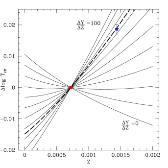
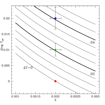
Figure 7: Left (right) panel: same as Figure 3 (4) for $\omega$Cen (NGC 2808), but using Eq. 4 with $P_{1}=1.5$.

We now re–interpret the split of the multiple MS of globular clusters by means of these empirical homology relations, with a re-calibrated $P_{1}=1.5$. Fig. 7 shows that the blue sequence of $\omega$Cen is now fitted with $\Delta Y/\Delta Z=75$ and $Y_{\rm{bMS}}=0.30$. For NGC 2808, the middle and blue MS are now fitted with $\Delta Y=0.02$ and $0.04$ respectively, corresponding to $Y_{\rm{mMS}}=0.27$ and $Y_{\rm{bMS}}=0.29$. These new values of the helium enrichment are significantly lower than the earlier estimates $Y\simeq=0.4$ and are within reasonable reach of extant theories on stellar nucleosynthesis and chemical evolution (e.g. Yi 2009).

To summarize: if we assume that the unique culprit of the erroneous broadening of the theoretical low–Z MS is the response of stellar structure to $\Delta Y/\Delta Z$, and consequently recalibrate the first term in the homology relations, the estimated $\Delta Y$ for the subpopulations of GC’s is drastically reduced. The new estimates of the helium content of the subpopulations are no longer extreme; rather, they are close to the solar helium content or slightly larger ($Y\leq 0.3$) which makes them relatively easy to reconcile with chemical evolution models.

5.2 Empirical calibration of the second term

An alternative way to bring the theoretical broadening of the low MS in agreement with observations, is to act on the second term of the homology relations in Eq. 4. As anticipated above, this term only depends on metallicity and therefore its alteration will have no impact on the interpretation of the multiple MS of globular clusters, where metallicity differences are minimal or vanishing. But for nearby K dwarfs and subdwarfs, the metallicity range is significant and exploring the effects of this second term is worthwhile.

It is clear from (Eq. 4) that parameters $P_{2}$ and $P_{3}$ are degenerate, in the sense that a given change in the second term can be obtained by modifying either of the two parameters. Fig. 8 shows that, fixing $P_{1}$, the best combined solution for $P_{2}$ and $P_{3}$ lies roughly along a hyperbola.

Therefore, we choose to discuss the role of the second term by optimizing $P_{3}$, which is an interesting parameter as it is significantly different between the theoretical and the numerical homology relations (Section 4).

Keeping $P_{1}$ and $P_{2}$ fixed to the values of Section 4, we find that $P_{3}\sim 150$ is the optimal value to obtain $\Delta Y/\Delta Z=2$ for nearby low–Z stars (Fig. 9). However, while we do obtain $\Delta Y/\Delta Z=2$ on average, compared to the case in Fig. 6 there is now considerable scatter and many stars remain with uncomfortably low helium abundances. It is intriguing, though, that the optimized value of $P_{3}$ is quite close to the theoretical value of 100.

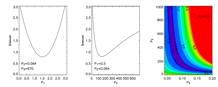
Figure 8: Left and central panel: reduced $\chi^{2}$ obtained fitting the K dwarfs in Casagrande et al. (2007) to Eq. 4, imposing $\Delta Y/\Delta Z=2$ and optimizing only one free parameter at a time. Right panel: contour lines for the reduced $\chi^{2}$ (values indicated by the labels) when only $P_{1}$ is fixed: the best solution for ($P_{2}$, $P_{2}$) lies along an hyperbola.

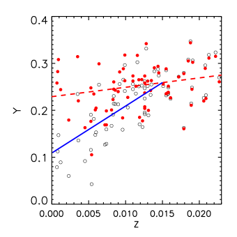
Figure 9: Same as Figure 6 but when operating on $P_{3}=150$ to obtain the $\Delta Y/\Delta Z=2$.

Notice that the cause of the discrepancy is entirely ascribed to some sort of metallicity dependence now. For instance, the variation of the mixing-length with $Z$ suggested in Casagrande et al. (2007) to avoid low helium abundances, in the framework of the homology relations can be formally described by the second term. The same can be said for any change in stellar models that would only respond to metallicity differences and not to differences in the helium content: it would have no impact on the interpretation of the multiple main sequences of Globular Clusters.

6 Summary and discussion

In this paper we draw attention on the possible connection between the HR diagram of globular clusters with multiple Main Sequences ($\omega$Cen and NGC 2808) and the broadening of the low MS defined by nearby stars. Although not “inverted” as in $\omega$Cen, where the metal-rich Main Sequence is bluer than the metal-poor one, the broadening defined by nearby subdwarfs is much narrower than expected for a standard helium content and helium–to–metal enrichment law $\Delta Y/\Delta Z\sim 2$. At low metallicities, $\Delta Y/\Delta Z\sim 10$ is formally necessary to reproduce the observed broadening, but this is unacceptable as it implies helium fractions much lower than the cosmological BBN floor.

It is worth remarking here that the results by Casagrande et al. (2007) on the broadening of the low MS were corroborated by the analysis of a number of binary stars, whose masses were well reproduced by theoretical isochrones — again at the expense of assuming, for some low Z binaries, sub-primordial helium abundances. Also, one may argue that the problem lies in an incorrect $T_{\rm{eff}}$ scale for low Z stars. Without entering here a detailed discussion on the robustness of the IRFM scale by Casagrande et al. (2006, 2010), suffice here to mention that this is one of the hottest scales available (as discussed in the original papers and in Sousa et al. 2008). It is hotter by 100 K than other IRFM renditions (the now superseded scales by Alonso, Arribas & Martinez–Roger 1996 and Ramírez & Meléndez 2005), and it is comparable within $\pm$50 K to various spectroscopic scales in the metallicity range relevant for this work.

Therefore, any other $T_{\rm{eff}}$ scale will just worsen the K dwarf problem, with real stars even cooler than the models. Also, it does not seem plausible that all the (independent) scales available are systematically offset by $>200$ K, which is what is needed to bring the K dwarfs of Casagrande et al. (2007) in line with stellar models.

We estimate the possible extent of the required revision of low MS stellar models on the base of homology relations. First we show that theoretical homology relations properly reproduce the response of stellar models to the helium content: in particular, analyzing the split of the multiple MS in $\omega$Cen and NGC 2808 by homology relations yields the same conclusions as full isochrone analysis (i.e. a helium content $Y\sim$ 0.4 for the blue subpopulations). Then, since both isochrones and theoretical homology relations fail the interpretation of the nearby low–Z Main Sequence, we calibrate empirical homology relations to yield consistently $\Delta Y/\Delta Z\sim 2$ for nearby stars, and inspect the consequences for the MS splits in globular clusters.

If we entirely impute the failure of the low-MS stellar models to a wrong response to the helium abundance (and correspondingly re-calibrate the helium–sensitive term of the homology relations), the consequences for globular clusters are highly significant: the helium content of the blue sub-populations is reduced from 40% to 30%, which is far easier to explain with chemical evolution models (Renzini 2008; Yi 2009).

Alternatively, if stellar models for the low MS are assumed to fail in their metallicity dependence (i.e. we re-calibrate only the homology term expressing the metallicity dependence of opacity) the consequences for globular clusters are negligible — as the metallicity differences between the subpopulations are minimal or vanishing.

As the solution for K dwarf models can be intermediate between these two extreme assumptions, we suggest that the helium rich populations in globular clusters are likely to have a helium content $Y$ in between 0.3–0.4; but altogether, there is room to decrease their estimated helium content from the extreme $Y=0.4$ that is the commonly quoted value.

In summary, the purpose of this exercise is to draw the attention of model–makers to the problem of the HR diagram of nearby low–Z stars: improvements in this respect are potentially important also for the riddle of the helium self-enrichment in globular clusters.

We remind indeed that, while a helium content as high as $Y\sim 0.35-0.4$ seems to nicely account for the multiple Main Sequences and the morphology of the Horizontal Branch (HB), other observations provide some counter-evidence for such a helium rich sub-population. In $\omega$Cen, the location of the RGB bumps of the metal–poor and metal–intermediate populations is consistent with a maximum $\Delta Y<0.1$, less than what is derived from MS and HB analysis (Sollima et al. 2005). Sollima et al. (2006) have also identified RR Lyræ stars with metallicity corresponding to that of the blue MS, but normal helium content — which would require the metal–intermediate population to be further split into a helium rich and a helium normal subcomponents.

NGC 6752 is another cluster suspected to host a helium enriched population, due to the morphology of its HB and the presence of a broadened, possible multiple MS (Milone et al. 2010); however, Villanova et al. (2009) did not detect large helium abundances in the spectra of blue HB stars in the (narrow but crucial) temperature range $8500<T_{\rm{eff}}<11500$, hot enough to produce helium lines but still unaffected by helium sedimentation. Other studies of clusters suspected to host helium rich sub-populations have not confirmed their presence (e.g. Lee et al. 2009 for NGC 1851; Catelan et al. 2009b for M3). While awaiting for independent proof of high helium abundances from direct spectral measurements or other features in the HR diagram (see the recent review by Catelan et al. 2009a), we remark that the helium abundances obtained by our proposed revision, $Y\raisebox{-3.8pt}{$\;\stackrel{{\scriptstyle\textstyle<}}{{\sim}}\;$}0.3$, are consistent with all of the above–mentioned constraints.

The need for sub-primordial helium abundances to fit a handful of nearby subdwarfs on the HR diagram was first noticed by Fernandes et al. (1998) and Lebreton et al. (1999) who advocated the inclusion of additional physical processes not implemented in standard stellar evolutionary calculations. In the following, we discuss a number of possible solutions to the problem. Broadly speaking, we can classify them as metallicity–dependent solutions, which shall not concern the helium rich populations of globular clusters, and helium–dependent solutions, which we expect also to impact the interpretation of globular clusters. We may add that, considering the nice agreement between the multiple MS and the HB morpology in $\omega$ Cen and NGC 2808, the optimal helium–dependent solution should preferably preserve this relation; this can be achieved if the new stellar models will not just shift the low metallicity ZAMS to lower effective temperatures, but also affect the luminosity of individual stars and accelerate their evolution, which helps to populate the blue side of the HB. Casagrande et al. (2007) discussed a number of possible solutions (all in the metallicity–dependent class). We briefly recall them and discuss a few more here below.

Mixing length

A mixing length parameter decreasing with metallicity would make low Z models redder; for the isochrones we used, the variation should be from the reference solar value $\alpha$=1.68 to $\alpha$=1.0 at low Z. While any dependence of $\alpha$ on metallicity, mass or other physical parameters is still highly disputed (Casagrande et al. 2007 and references therein) this solution would have no consequence for the helium content of globular clusters, as it is metallicity dependent and does not significantly affect the luminosity and lifetime of the stellar models.

Diffusion + non–LTE effects

Element diffusion affects the location of low MS stars in the HR diagram: it makes stellar models redder, and moreover it lowers the measured surface metallicity with respect to the real intrinsic one. In this scenario, low Z subdwarfs look redder than we expect, mostly because they are actually more metal rich than we measure. Casagrande et al. (2007) discussed this possibility resorting to literature models with fully efficient (“maximal”) diffusion, and found that it does not completely solve the problem, unless it is combined with additional errors on the observed metallicity due to non–LTE effects. (This solution also would have no effect on globular clusters, since it is metallicity and age dependent, and the gap in both is small for the multiple populations of globular clusters.)

However, as discussed in that paper, there is evidence that both of these mechanisms are not fully efficient in real stars, as one would need to solve the K dwarf problem. For diffusion in particular, observations of field and cluster metal-poor dwarfs point toward inhibited efficiency and additional — yet ad hoc — processes are nowadays invoked to contrast diffusion (e.g. Chaboyer et al. 2001; Richard, Michaud & Richer 2002, 2005; Korn et al. 2007).

Boundary conditions

also play a role in stellar evolutionary tracks. A solar scaled $T-\tau$ relation provides a good description of the atmospheric structure also in metal-poor stars, and may contribute to improve low Z models with respect to gray atmosphere boundary conditions. However, the effect appears to be quite small for MS stars, when each set of isochrones consistently adopts a mixing length parameter calibrated on the solar model (Vandenberg et al. 2008).

Besides, boundary conditions are expected to become more relevant at lower stellar masses and luminosities (due to the deeper surface convection), while in Casagrande et al. (2007) we verified that there is no systematic trend of the derived $\Delta Y/\Delta Z$ with $M_{bol}$.

Also this solution relies on a metallicity–dependent effect and would not bring substantial revisions to the helium content in the multiple MS of GCs.

Convection

One can always consider changing the boundary of convective regions as a viable working hypothesis. (In fact, the very presence of a convective envelope renders real K dwarfs not rigorously representable by homology relations.) Considering that the convective envelope gets thinner at lower metallicities, any change in the convection scheme (e.g. extra-mixing, or undershooting) is expected to affect solar metallicity objects more, creating a differential effect in metallicity that could change the relative location of the low MS as a function of Z. Also this solution falls in the metallicity-dependent category and is not expected to impact on the GC analysis.

Opacity

As K dwarfs are largely radiative structures, in particular in the regions where nuclear energy is produced, opacity is a leading ingredient in determining their luminosity. An incorrect metallicity dependence of opacity would seriously affect the broadening of the low MS. The idea is tempting, as the “break” in the estimated $\Delta Y/\Delta Z$ occurs close to $Z_{0}=0.01$, which is the classic divide between free-free and bound-free dominated opacity in stellar interiors (Cox & Giuli 2004). The parameter $P_{3}$ in the original homology relations is related to this characteristic metallicity as $P_{3}=1/Z_{0}$ (Section 4 and Appendix) and we have seen that modern isochrones are better described by $P_{3}\simeq 670$ rather than 100, effectively reducing $Z_{0}$ to 0.0015 (Section 4; Pagel & Portinari 1998). However, optimizing empirical homology relations on the opacity term, restores a value for $P_{3}$ or $Z_{ff/bf}$ closer to the theoretical one ($P_{3}=150$ or $Z_{0}\simeq 0.007$). This suggests that the culprit might be the metallicity dependence of opacity (which would then be irrelevant for globular clusters). It is easier to figure errors in the bound-free contribution to opacity, rather than in the free-free component, at least for the bulk of the star wher H and He are completely ionized. Lowering the bound-free contribution to opacity would imply a recalibration of solar metallicity isochrones, after which high Z (bound-free dominated) and low Z (free-free dominated) model MS may fall closer to each other, thus reducing the broadening. However, we wonder if there is much room for profound changes in opacity, given the excellent agreement between the major current, independent databases (Opacity Project, Seaton 2005 and references therein; and OPAL, Iglesias & Rogers 1996 and references therein) and keeping in mind that improvement in atomic data, input physics etc. most often leads to an increase in the opacity, as more and more opacity sources are taken into account. Helioseismology has shown extant OPAL and OP opacities to be fully adequate for Solar models with the “classic” solar composition; while an increase in opacity by 10–20% in a suitable temperature range has been invoked for the Solar model with new, lower metallicity — possibly in connection with increased neon abundance (Basu & Antia 2008; Asplund et al. 2009; Serenelli et al. 2009; and references therein). How these or other fundamental changes of the Solar model, to recover agreement with helioseismological constraints, will impact low Z subdwarfs and the relative location of MS of subsolar metallicity on the HR diagram, remains to be explored.

Finally, we notice that the “helium problem” may not be limited to K dwarfs: systematic temperature offsets from the theoretical Main Sequence at low Z have been highlighted for FG dwarfs in the Geneva–Copenhagen survey (Nördstrom et al. 2004); and a helium content Y=0.23–0.24 (i.e. slightly sub-cosmological) has been recently suggested for a slighly metal-poor F dwarf binary ([Fe/H]=–0.25; Clausen et al. 2010). If the problem indeed extends to FG dwarfs, clearly some of the suggested solutions (for instance, those related to diffusion) are not viable.

All of the solutions suggested above rely, more or less indirectly, on metallicity dependence; this is the standard way we think of stellar models. However, our exercise in this paper highlights that it is worth thinking of other possible systematics in the stellar models, especially connected to the helium abundance, for their interesting impact on the multiple MS of globular clusters.

As mentioned above, opacity has a key role in the structure of lower MS stars, so we may wonder whether the issue can be the helium dependence of opacity. This can be hardly modified in regions of complete ionization; more promising are regions where He is partially recombined and contributes to the boud-free opacity.

Other helium–dependent effects may be considered, such as diffusion mechanisms that would act differently for helium as for metals. (However, preliminary tests on only–helium diffusion seem to go in the opposite direction as needed for globular clusters, with the helium rich MS getting proportionally more red than the helium poor; A. Serenelli, priv. comm.)

Possibly, other of the above mentioned solutions (mixing length, convection etc.) can be recast and explored in terms of helium dependence, rather than metallicity dependence. Any ideas in this direction are highly desired: hopefully, astrophysicists will be as creative in solving the problem of the HR diagram of low metallicity K dwarfs, as they have been in tackling the riddle of the extreme helium rich populations in globular clusters!

Appendix A Homology relations — the background

An excellent introduction of the homology relations used in this paper is given by Fernandes et al. (1996), which we follow. A family of permanently homologous stars (i.e., stars with the same relative mass distribution, that are in hydrodynamical and thermal equilibrium) can be obtained in the hypothesis that the equation of state is the perfect gas law, and that opacity and energy generation rate follow laws of the kind:

$$\kappa=\kappa_{0}\,\rho^{n}T^{-s}$$

$$\epsilon=\epsilon_{0}\,\rho^{\lambda}T^{\nu}$$

(Cox & Giuli 1968). Other underlying assumptions are that the energy transport occurs via radiative diffusion over most of the interior (in particular, over the energy generation region, as is the case for the low MS) and that the radial profile of chemical composition differs, in different stars, just by a scale factor. The latter assumption holds in particular for stars on the ZAMS, with internally uniform chemical composition.

For low–mass MS stars, opacity is dominated by bound–free and free-free processes and well approximated by Kramer’s law: $\kappa=\kappa_{0}\rho T^{-3.5}$; while the energy generation rate via pp chain approximately follows $\epsilon_{pp}=\epsilon_{0}\rho T^{4}$. With these dependencies on $\rho$ and $T$, homology transformations yield the following relation for the luminosity and effective temperature of the star

$$L=\epsilon_{0}^{-0.077}\mu^{7.769}\kappa_{0}^{-1.077}M^{5.462}$$

$$T_{\rm{eff}}=\epsilon_{0}^{-0.096}\mu^{2.211}\kappa_{0}^{-0.346}M^{1.327}$$

as a function of mass $M$ and molecular weight $\mu$. Eliminating mass, one derives:

$$L=\epsilon_{0}^{0.318}\,\mu^{-1.332}\,\kappa_{0}^{0.347}\,T_{\rm{eff}}^{4.116}$$ (5)

The last factor indicates the slope of the ZAMS for a given chemical composition: about 10 mag per dex in log($T_{\rm{eff}}$) — flatter than, but not so far from, the slope obtained with detailed stellar structure computations (17 mag per dex, Section 2). Here we are mostly interested in the broadening of the ZAMS in luminosity as a function of chemical composition, at a fixed $T_{\rm{eff}}$; such broadening is expressed by the first three factors. Since H–burning occurs via the p-p chain:

$$\epsilon_{0}\propto X^{2}$$

The molecular weight $\mu$, throughout most of the star where complete ionization applies, is given by:

$$\mu^{-1}=2X+\frac{3}{4}Y+\frac{1}{2}Z=\frac{1}{4}(3+5X-Z)$$

For bound–free and free–free opacity, approximately: $\kappa_{0,bf}\approx 7.40\times 10^{24}\times\frac{5}{10}Z(1+X)$, $\kappa_{0,ff}\approx 3.76\times 10^{22}(1+X)$ (Cox & Giuli 2004), so that

$$\kappa_{0}=\kappa_{0,bf}+\kappa_{0,ff}\propto(1+X)(100Z+1)$$

Notice that $Z_{0}=\frac{1}{100}$ is where opacity drifts from free-free dominated ($Z<0.01$) to bound-free dominated ($Z>0.01$). Altogether, we can write the homology relation (5) as:

$$L={\cal F}(\epsilon_{0},\mu,\kappa_{0})\;T_{\rm{eff}}^{4.116}$$

with

$${\cal F}\propto X^{0.636}\,(3+5X-Z)^{1.332}\,(1+X)^{0.347}(100Z+1)^{0.347}$$

The first factor in the $\cal F$ function is related to the energy generation rate, the second factor to the molecular weight, and the last two factors to opacity. It is then straightforward to derive Eq. 1 for the broadening of the ZAMS in luminosity, with respect to a reference composition $(X_{r},Y_{r},Z_{r})$:

$$\Delta M_{\rm{Bol}}=-2.5\log\frac{L}{L_{r}}=-2.5\log\frac{{\cal F}(X,Y,Z)}{{\cal F}(X_{r},Y_{r},Z_{r})}$$

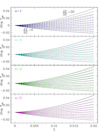
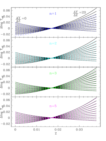
Figure 10: Homology relations for $\frac{\Delta Y}{\Delta Z}$ ranging from 0 to 20 (with a pace of 2) as indicated. Coloured dashed lines represent the approximate relations of Eq. 7 for increasing order of the terms of the expansion. The true relations are well reproduced up to $\frac{\Delta Y}{\Delta Z}=20$ for $n>2$ — at least within a metallicity range $\Delta Z\stackrel{{\scriptstyle\textstyle<}}{{\sim}}0.02$. The dotted line shows our simplified form of the homology relations (Eq. 3).

A.1 Polynomial approximations

Pagel & Portinari (1998) suggested an approximation of the homology relations based on Taylor series expansion of the terms in $\log(1-x)$:

$$\log(1-x)=-\frac{1}{\ln 10}\sum_{n=1}^{\infty}\frac{x^{n}}{n}\leavevmode\nobreak\ \leavevmode\nobreak\ \leavevmode\nobreak\ \leavevmode\nobreak\ \leavevmode\nobreak\ \leavevmode\nobreak\ \leavevmode\nobreak\ \leavevmode\nobreak\ \leavevmode\nobreak\ \leavevmode\nobreak\ \leavevmode\nobreak\ \leavevmode\nobreak\ \leavevmode\nobreak\ \leavevmode\nobreak\ \leavevmode\nobreak\ \leavevmode\nobreak\ \leavevmode\nobreak\ \leavevmode\nobreak\ |x|<1$$

Expansion to first order of Eq. 2 yields a linearized formula similar to eq. 5 of Pagel & Portinari:

$$\begin{array}[]{l}\vskip 6.0pt plus 2.0pt minus 2.0pt\Delta\log{T_{\rm{eff}}}^{(1)}=-0.051\log\left(\frac{100Z+1}{100Z_{r}+1}\right)\\ \vskip 6.0pt plus 2.0pt minus 2.0pt\;\;\;\;\;\;\;\;\;\;\;\;\;\;+\left[\frac{0.0406}{X_{r}}+\frac{0.02215}{1+X_{r}}+\frac{0.4256}{3+5X_{r}-Z_{r}}\right]\delta(Z-Z_{r})\\ \;\;\;\;\;\;\;\;\;\;\;\;\;\;+\frac{0.08512}{3+5X_{r}-Z_{r}}(Z-Z_{r})\\ \end{array}$$ (6)

(where the last term is negligible). However this linearized approximation holds only for $|\delta(Z-Z_{r})|<<1$ and does not recover very well the original homology relations for $\frac{\Delta Y}{\Delta Z}>5$ (see Fig. A1).

One can then resort to further terms in the expansion. The second order terms yield:

$$\begin{array}[]{l}\vskip 6.0pt plus 2.0pt minus 2.0pt\Delta\log{T_{\rm{eff}}}^{(2)}=\Delta\log{T_{\rm{eff}}}^{(1)}\\ \vskip 6.0pt plus 2.0pt minus 2.0pt\;\;\;\;\;\;\;\;\;\;\;\;\;\;\;+\left[\frac{0.0203}{X_{r}^{2}}+\frac{0.01107}{(1+X_{r})^{2}}+\frac{1.064}{(3+5X_{r}-Z_{r})^{2}}\right]\delta^{2}(Z-Z_{r})^{2}\\ \vskip 6.0pt plus 2.0pt minus 2.0pt\;\;\;\;\;\;\;\;\;\;\;\;\;\;\;+\frac{0.4256}{(3+5X_{r}-Z_{r})^{2}}\,\delta\,(Z-Z_{r})^{2}\\ \;\;\;\;\;\;\;\;\;\;\;\;\;\;\;+\frac{0.04256}{(3+5X_{r}-Z_{r})^{2}}\,(Z-Z_{r})^{2}\\ \end{array}$$

where the last two terms are negligible. The third order expansion terms yield:

$$\begin{array}[]{l}\vskip 6.0pt plus 2.0pt minus 2.0pt\Delta\log{T_{\rm{eff}}}^{(3)}=\Delta\log{T_{\rm{eff}}}^{(2)}+\\ \vskip 6.0pt plus 2.0pt minus 2.0pt\;\;\;\;\;\;\;\;\;\;\;\;\;\;\;\left[\frac{0.01354}{X_{r}^{3}}+\frac{0.00738}{(1+X_{r})^{3}}+\frac{3.547}{(3+5X_{r}-Z_{r})^{3}}\right]\delta^{3}(Z-Z_{r})^{3}\\ \vskip 6.0pt plus 2.0pt minus 2.0pt\;\;\;\;\;\;\;\;\;\;\;\;\;\;\;+\frac{0.2128}{(3+5X_{r}-Z_{r})^{3}}\,\delta^{2}\,(Z-Z_{r})^{3}\\ \vskip 6.0pt plus 2.0pt minus 2.0pt\;\;\;\;\;\;\;\;\;\;\;\;\;\;\;+\frac{0.4256}{(3+5X_{r}-Z_{r})^{3}}\,\delta\,(Z-Z_{r})^{2}\\ \;\;\;\;\;\;\;\;\;\;\;\;\;\;\;+\frac{0.0284}{(3+5X_{r}-Z_{r})^{3}}\,(Z-Z_{r})^{3}\\ \end{array}$$

where the last three terms are negligible. In general, neglecting the smaller terms of the kind $\delta^{m}(Z-Z_{r})^{n}$ with $m<n$, we can write the following polynomial approximation to homology relations:

$$\begin{array}[]{l}\vskip 6.0pt plus 2.0pt minus 2.0pt\Delta\log T_{\rm{eff}}\simeq-0.051\log\left(\frac{100Z+1}{100Z_{r}+1}\right)\\ +\sum_{n=1}^{\infty}\left[\frac{0.0406}{X_{r}^{n}}+\frac{0.02215}{(1+X_{r})^{n}}+\frac{0.08512}{(3+5X_{r}-Z_{r})^{n}}\right]\frac{\delta^{n}(Z-Z_{r})^{n}}{n}\\ \end{array}$$ (7)

The corresponding parametric fitting formula for the isochrones would be of the kind:

$$\Delta\log T_{\rm{eff}}\simeq-a_{1}\log\left(\frac{a_{2}Z+1}{a_{2}Z_{r}+1}\right)+\sum_{n=1}^{\infty}b_{n}\delta^{n}(Z-Z_{r})^{n}$$ (8)

For $n$-th order series expansion, this fitting formula has $n+2$ free parameters. Pagel & Portinari (1998) indeed used a linearized approximation ($n=1$) similar to Eq. 6 as a guideline, and had 3 parameters in their fitting formula for isochrones.

Fig. A1 shows that expansion to order $n>2$ is needed to yield a good fit up to $\Delta Y/\Delta Z\sim 10$ (at least in the range $0\leq Z$ $\;\stackrel{{\scriptstyle\textstyle<}}{{\sim}}\;$$Z_{\odot}$) needed for the study of nearby K dwarfs of low Z. Our simplified form of the original homology relations (Eq. 3) performs as well as the $n=3$ order of series expansion, with just 3 free parameters in the corresponding fitting formula.

For extremely high $\Delta Y/\Delta Z$, as applies to the case of $\omega$Cen, it is worth using the original formulation of the homology relations (Eq. 2), which indeed we showed in Section 3 to yield excellent results when applied to the multiple MS of $\omega$Cen amd NGC 2808. Notice, in fact, that for very high $\Delta Y/\Delta Z$ the basic condition for Taylor series expansion, $|x|=|\delta(Z-Z_{r})|<1$, may no longer be fulfilled.

Appendix B Updated Hipparcos parallaxes

For simplicity this paper relies on the helium abundances determined by Casagrande et al. (2007); in the meantime, the HR diagram of nearby stars has been revised with updated Hipparcos parallaxes (van Leewven 2007). In Fig. B1 we show that the effect of the revised parallaxes is minimal: the sample only slightly changes (3 stars are now rejected by the parallax limit 6%, while 5 new stars are included, for a total of 88 objects) and the trend toward significantly sub-cosmological Y values is confirmed. Nor it appears to be due to low metallicity stars being systematically more distant than the solar metallicity ones (with systematically intrinsic bluer colours due to neglected reddening): though a slight distance–metallicity trend is present as expected, most of the stars lie within 30 pc for all metallicities (Fig. B2). Also, in Fig. 1 we show that the reddening/extinction correction needed to reconcile metal-poor stars with isochrones would correspond to $E(B-V)$=0.10, which is certainly too extreme for so nearby stars.

Other possible systematics have been carefully checked and excluded in Casagrande et al. (2007). We do not deem necessary here to repeat the detailed Monte–Carlo simulations performed in 2007 to estimate realistic errorbars (shown in Fig. 5), since it suffices here to demonstrate that the new parallaxes by no means solve the riddle of sub-cosmological helium abundances.

Finally, we have also verified that the updated temperature scale by Casagrande et al. (2010) also does not significantly change the Y(Z) plot.

Figure 11: Helium plot for the sample by Casagrande et al. (2007) (stars) versus the update sample with the revised parallaxes of van Leewven (2007) (squares)

Figure 12: Distances and metallicities of sample stars from Casagrande et al. (2007) (top panel) and for the updated sample with the revised parallaxes of van Leewven (2007)(bottom panel)

References

- [1] Alonso A., Arribas S., Martinez-Roger C., 1996, A&AS 117, 227
- [2] Anderson J., Piotto G., King I.R., Bedin L.R., Guhathakurta P., 2009, ApJ 697, L58
- [3] Asplund M., Grevesse N., Sauval A.J., Scott P., 2009, ARA&A, 47, 481
- [4] Balser D.S., 2006, AJ 132, 2326
- [5] Basu S., Antia H.M., 2008, Phys. Rep. 457, 217
- [6] Bedin L.R., Piotto G., Anderson J., Cassisi S., King Y.R., Momany Y., Carraro G., 2004, ApJ 605, 125
- [7] Bellazzini M., Ferraro F.R., Sollima A., Pancino E., Origlia L., 2004, A&A 424, 199
- [8] Bertelli G., Girardi L., Marigo P., Nasi E., 2008, A&A 484, 815
- [9] Boyajian T.S., McAlister H.A., Baines E.K., et al. 2008, ApJ 683, 424
- [10] Caloi V., D’Antona F., 2005, A&A 435, 987
- [11] Caloi V., D’Antona F., 2007, A&A 463, 949
- [12] Carigi L., Peimbert M., 2008, RMxAA 44, 341
- [13] Carretta E., Bragaglia A., Gratton R.G., Leone F., Recio-Blanco A., Lucatello S., 2006, A&A 450, 523
- [14] Carretta E., Bragaglia A., Gratton R.G., D’Orazi V., Lucatello S., 2009, A&A in press (arXiv:0910.0675)
- [15] Casagrande L., 2008, PhD Thesis, University of Turku
- [16] Casagrande L., Portinari L., Flynn C., 2006, MNRAS 373, 13
- [17] Casagrande L., Flynn C., Portinari L., Girardi L., Jimenez J., 2007, MNRAS 382, 1516
- [18] Casagrande L., Ramírez I., Meléndez J., Bessel M., Asplund M., 2010, A&A in press (arXiv:1001.3142)
- [19] Castellani V., Degl’Innocenti S., Marconi M., 1999, A&A 349, 834
- [20] Catelan M., Valcarce A.A.R., Sweigart A.V., 2009a, IAU Symp. 266, eds. R. de Grijs and J.R.D. Lepine (arXiv:0910.1367)
- [21] Catelan M., Grundahl F., Sweigart A.V., Valcarce A.A.R., Cortés C., 2009b, ApJ 695, L97
- [22] Chaboyer B., Fenton W.H., Nelan J.E., Patnaude D.J., Simon F.E., 2001, ApJ 562, 521
- [23] Chiosi C., Matteucci M., 1982, A&A 105, 140
- [24] Choi E., Yi S.-K., 2007, MNRAS 375, L1
- [25] Choi E., Yi S.-K., 2008, MNRAS 386, 1332
- [26] Clausen J.V., Olsen E.H., Helt B.E., Claret A., 2010, A&A in press (arXiv:0912.3108)
- [27] Cox J.P., Giuli R.T., 1968, Principles of Stellar Structure - Volume II. Gordon & Breach Science Publishers, New York
- [28] Cox J.P., Giuli R.T., 2004, Principles of Stellar Structure. Extended Second Edition by A. Weiss, W. Hillebrandt, H.-C. Thomas and H. Ritter, Cambridge Scientific Publishers, Cambridge, UK
- [29] D’Antona F., Caloi V., 2004, ApJ 611, 871
- [30] D’Antona F., Bellazzini M., Caloi V., Pecci F.F., Galleti S., Rood R.T., 2005, ApJ 631, 868
- [31] Del Principe M., Piersimoni A.M., Storm J., et al. 2006, ApJ 652, 362
- [32] Faulkner J., 1967, ApJ 147, 617
- [33] Fernandes J., Lebreton Y., Baglin A., 1996, A&A 311, 127
- [34] Fernandes J., Lebreton Y., Baglin A., Morel P., 1998, A&A 338, 455
- [35] Fukugita M., Kawasaki M., 2006, ApJ 646, 691
- [36] Harris W.E., 1996, AJ 112, 1487
- [37] Iglesias J.A., Rogers F.J., 1996, ApJ 464, 943
- [38] Izotov Y.I., Thuan T.X., Stasinska G., 2007, ApJ 662, 15
- [39] Jimenez R., Flynn C., McDonald J., Gibson B., 2003, Science 299, 1552
- [40] Karakas A., Fenner Y., Sills A., Campbell S.W., Lattanzio J., 2006, ApJ 652, 1240
- [41] Korn A.J., Grundahl F., Richard O., Barklem P.S., Mashonkina L., Collet, R., Piskunov N., Gustafsson B., 2006, Nat 442, 657
- [42] Korn A. J., Grundahl F., Richard O., Mashonkina L., Barklem P.S., Collet R., Gustafsson B., Piskunov N., 2007, ApJ 671, 402
- [43] Lebreton Y., Perrin M.-N.,, Cayrel R., Baglin A., Fernandes J., 1999, A&A 350, 587
- [44] Lee Y.-W., Joo S.-J., Han S.-I., et al. 2005, ApJ 621, L57
- [45] Lee J.-W., Lee J., Kang Y.-W., et al. 2009, ApJ 695, L78
- [46] van Leeuwen F., 2007, A&A 474, 653
- [47] Lub J., 2002, in Centauri: a unique window into astrophysics, ed. F. van Leeuwen, J. Hughes, G. Piotto, (San Francisco:ASP), ASP Conf. Ser. 265, p. 95
- [48] Marcolini A., Gibson B.K., Karakas A.I., Sánchez–Blázquez P., 2009, MNRAS 395, 719
- [49] Maeder A., 1992, A&A 264, 105
- [50] Maeder A., Meynet G., 2006, A&A 448, L37
- [51] Michaud G., Vauclair G., Vauclair S., 1983, ApJ 267, 256
- [52] Michaud G., Richer J., Richard O., 2008, ApJ 675, 1223
- [53] Milone A.P., Piotto G., King I.R., et al. 2010, ApJ 709, 1183
- [54] Norris J.E., 2004, ApJ 612, 25
- [55] Nordström B., Mayor M., Andersen J., et al. 2004, A&A 418, 989
- [56] Pagel B.E.J., Portinari L., 1998, MNRAS 298, 747
- [57] Peimbert M., 2003, ApJ 584, 735
- [58] Peimbert M., Luridiana V., Peimbert A., 2007, ApJ 666, 636
- [59] Peng F., Nagai D., 2009, ApJL 705, L58
- [60] Perrin M.-N., de Strobel G.C., Cayrel R., Hejlesen P.M., 1977, A&A 54, 779
- [61] Piotto G., 2009, IAU Symp. 258 in press (arXiv:0902.1422)
- [62] Piotto G., Villanova S., Bedin L.R., Gratton R., Cassisi S., et al. 2005, ApJ 621, 777
- [63] Piotto G., Bedin L.R., Anderson J., King I.R., Cassisi S., et al. 2007, ApJ 661, L53
- [64] Prantzos N., Charbonnel C., 2006, A&A 458, 135
- [65] Ramírez I., Meléndez J., 2005, ApJ 626, 446
- [66] Renzini A., 2008, MNRAS 391, 354
- [67] Richard O., Michaud G., Richer J., 2002, ApJ 580, 1100
- [68] Richard O., Michaud G., Richer J., 2005, ApJ 619, 538
- [69] Romano D., Matteucci F., Tosi M., Pancino E., Bellazzini M., Ferraro F., Limongi M., Sollima A., 2007, MNRAS 376, 405
- [70] Romano D., Tosi M., Cignoni M., Matteucci F., Pancino E., Bellazzini M., 2009, MNRAS in press (arXiv:0910.1299)
- [71] Salaris M., Weiss A., Ferguson J.W., Fusilier D.J., 2006, ApJ 645, 1131
- [72] Seaton M.J., 2005, MNRAS 362, L1
- [73] Serenelli A., Basu S., Ferguson J.W., Asplund M., 2009, ApJ 705, L123
- [74] Sirianni M., Jee M.J., Benítez N., et al. 2005, PASP 117, 1049
- [75] Sollima A., Ferraro F.R., Pancino E.,, Bellazzini M., 2005, MNRAS 357, 265
- [76] Sollima A., Borissova J., Catelan M., Smith H.A., Minniti D., Cacciari C., Ferraro F.R., 2006, ApJ 640, L43
- [77] Sollima A., Ferraro F.R., Bellazzini M., Origlia L., Straniero O., Pancino E., 2007, ApJ 654, 915
- [78] Sousa S.G., Santos N.C., Mayor M., 2008, A&A 487, 373
- [79] Steigman G., 2007, Annual Review of Nuclear and Particle Systems, 57, 463
- [80] Torres G., Boden A., Latham D.W., Pan M., Stefanik R.P., 2002, AJ, 124, 1716
- [81] VandenBerg D.A., Edvardsson B., Eriksson K., Gustafsson B., 2008, ApJ 675, 746
- [82] Villanova S., Piotto G., Gratton R.G., 2009, A&A in press (arXiv:0903.3924)
- [83] Villanova S., Piotto G., King I.R., Anderson J., Bedin L.R., et al. 2007, ApJ 663, 296
- [84] Yi S.-K., 2009, IAU Symp. 258, eds. 253
- [85] Yi S., Demarque P., Kim Y.C., Lee Y.W., Ree C.H., Lejeune T., Barnes S., 2001, ApJS, 136, 417