Oscillations of weakly viscous conducting liquid drops in a strong magnetic field

Abstract

We analyse small-amplitude oscillations of a weakly viscous electrically conducting liquid drop in a strong uniform DC magnetic field. An asymptotic solution is obtained showing that the magnetic field does not affect the shape eigenmodes, which remain the spherical harmonics as in the non-magnetic case. Strong magnetic field, however, constrains the liquid flow associated with the oscillations and, thus, reduces the oscillation frequencies by increasing effective inertia of the liquid. In such a field, liquid oscillates in a two-dimensional (2D) way as solid columns aligned with the field. Two types of oscillations are possible: longitudinal and transversal to the field. Such oscillations are weakly damped by a strong magnetic field – the stronger the field, the weaker the damping, except for the axisymmetric transversal and inherently 2D modes. The former are overdamped because of being incompatible with the incompressibility constraint, whereas the latter are not affected at all because of being naturally invariant along the field. Since the magnetic damping for all other modes decreases inversely with the square of the field strength, viscous damping may become important in a sufficiently strong magnetic field. The viscous damping is found analytically by a simple energy dissipation approach which is shown for the longitudinal modes to be equivalent to a much more complicated eigenvalue perturbation technique. This study provides a theoretical basis for the development of new measurement methods of surface tension, viscosity and the electrical conductivity of liquid metals using the oscillating drop technique in a strong superimposed DC magnetic field.

1 Introduction

Shape oscillations of levitated metal droplets can be used to measure the surface tension and viscosity of liquid metals (Rhim et al. 1999; Egry et al. 2005). Theoretically, the former determines the frequency, while the latter accounts for the damping rate of oscillations. In the reality, experimental measurements may be affected by several side-effects. Firstly, levitated drops may be significantly aspherical and the oscillations amplitudes not necessarily small, whereas the classical theories describing the oscillation frequencies (Rayleigh 1945) and damping rates (Lamb 1993; Chandrasekhar 1981; Reid 1960) assume small-amplitude oscillations about an ideally spherical equilibrium shape. Corrections due to the drop asphericity have been calculated by Cummings & Blackburn (1991) and Suryanarayana & Bayazitoglu (1991). Bratz & Egry (1995) find the same order correction to the damping rate resulting also from AC-magnetic field. The effect of a moderate amplitude on the oscillations of inviscid drops has been analysed by Tsamopoulos & Brown (1983) who find that the oscillation frequency decreases with the square of the amplitude. Using a boundary-integral method, Lundgren & Mansour (1991) show that small viscosity has a relatively large effect on the resonant-mode coupling phenomena in the nonlinear oscillations of large axially symmetric drops in zero gravity. Numerical simulation of large-amplitude axisymmetric oscillations of viscous liquid drop by Basaran (1992), who uses the Galerkin/finite-element technique, shows that a finite viscosity results in a much stronger mode coupling than predicted by the small-viscosity approximation.

Secondly, the measurements may strongly be disturbed by AC-driven flow in the drop. The mode coupling by the internal circulation in axisymmetrically oscillating drop has been studied numerically by Mashayek & Ashgriz (1998) using the Galerkin/finite-element technique. To reduce the strength of the AC field necessary for the levitation and, thus, to minimise the flow, experiments may be conducted under the microgravity conditions during parabolic flights or on the board of space station (Egry et al. 1999). A cheaper alternative might be to apply a sufficiently strong DC magnetic field that can not only stabilise AC-driven flow but also suppress the convective heat and momentum transport responsible for the mode coupling under the terrestrial conditions as originally shown by Shatrov et al. (2003). Such an approach has been implemented first by Yasuda et al. (2004) on the electromagnetically levitated drops of Copper and Nickel which were submitted to a DC field of the induction up to $10\,T.$ The only motion of $Cu$ drops observed to persist in magnetic field above $1\,T$ was a solid-body rotation about an axis parallel to the magnetic field. No shape oscillations, usually induced by the AC-driven flow fluctuations, were observed. Note that this implies only the suppression of AC-driven flow but not of the shape oscillations themselves which require an external excitation to be observable. Yasuda et al. (2005) study the effect of suppression of the melt flow on the structure of various alloys obtained by the electromagnetic levitation melting technique in a strong superimposed DC magnetic field. The use of high magnetic fields in various material processing applications is reviewed by Yasuda (2007).

Note that a similar suppression of AC-driven flow can also be achieved by a fast spinning of the drop (Shatrov et al. 2007) that may be driven by an electromagnetic spin-up instability (Priede & Gerbeth 2000, 2006). The effects of both the drop rotation and AC-driven flow on the frequency spectrum of shape oscillations have been modelled numerically by Bojarevics & Pericleous (2009). Watanabe (2009) demonstrates numerically that a large enough oscillation amplitude can compensate for the effect of rotation on the frequency shift.

A novel method of measuring thermal conductivity of liquid silicon using the electromagnetic levitation in a strong superimposed DC magnetic has been introduced by Kobatake et al. (2007). Subsequent numerical modelling by Tsukada et al. (2009) shows that applying a DC magnetic field of $4\,T$ can suppress convection in molten silicon droplet enough to measure its real thermal conductivity. Later on this method has been extended to the measurements of heat capacity of molten austenitic stainless steel (Fukuyama et al. 2009) and also that of supercooled liquid silicon (Kobatake et al. 2010).

In order to determine the surface tension and viscosity or the electrical conductivity one needs to relate the observed surface oscillations with the relevant thermophysical properties of the liquid. General small-amplitude shape oscillations of conducting drop in a uniform DC magnetic field have been analysed first by Gailitis (1966). Although a magnetic field of arbitrary strength is considered, the solution is restricted to inviscid drops. Moreover, only the frequency spectrum and magnetic damping rates are found but not the associated shape eigenmodes, which may be useful for experimental identification of the oscillation modes. Energy dissipation by axisymmetric oscillations of a conducting drop in a weak DC magnetic field is considered by Zambran (1966), who finds the magnetic damping rates in agreement with more general results of Gailitis (1966). Axisymmetric oscillations of an electromagnetically levitated drop of molten $Al$ in a superimposed DC magnetic field are modelled numerically by Bojarevics & Pericleous (2003). A moderate DC magnetic field is shown to stabilise AC-driven flow and, thus, to eliminate the associated shape oscillations. A three-dimensional numerical simulation of an oscillating liquid metal drop in a uniform static magnetic field has been carried out by Tagawa (2007). The numerical results show that vertical magnetic field effectively damps the flow, while horizontal field tries to render the flow two-dimensional.

In the present paper, we analyse free oscillations of a viscous electrically conducting drop in a homogeneous DC magnetic field. In contrast to Gailitis (1966), we assume the viscosity to be small but non-zero and the magnetic field to be strong. This allows us to obtain an asymptotic solution to the eigenvalue problem for general small-amplitude 3D shape oscillations including the eigenmodes left out by Gailitis (1966), which are necessary for the subsequent determination of the viscous damping. Firstly, we show that the eigenmodes of shape oscillations are not affected by strong magnetic field. Namely, they remain the spherical harmonics as in the non-magnetic case. The magnetic field, however, changes the internal flow associated with the surface oscillations and, thus, the frequency spectrum. As the drop oscillates in a strong magnetic field, the liquid moves as solid columns aligned with the field. Two types of such oscillations are possible: longitudinal and transversal to the magnetic field. The oscillations are weakly damped by a strong magnetic field, except for both the axisymmetric transversal and inherently 2D modes. The former are magnetically overdamped because the incompressibility constraint does not permit an axially uniform radial flow. The latter, which are transversal modes defined by the spherical harmonics with equal degree and order, $l=m$, are not affected at all because these modes are naturally invariant along the field. Because the magnetic damping for all other modes decreases inversely with the square of the field strength, the viscous damping may become important in a sufficiently strong magnetic field.

The paper is organised as follows. The problem is formulated in $\S$2. Section 3 presents an inviscid asymptotic solution which yields the shape eigenmodes and frequency spectrum of longitudinal and transversal oscillations. Magnetic damping is found in $\S$3.2 as a next-order asymptotic correction to the frequency. Viscous damping rates are calculated in $\S$3.3 first by the eigenvalue perturbation technique for the longitudinal modes and then by an energy dissipation approach for both of the oscillation modes. The paper is concluded by a summary and discussion of the results in $\S$4.

2 Problem formulation

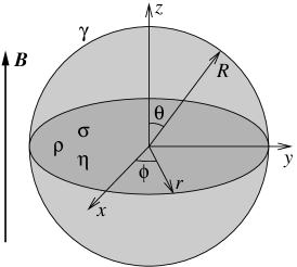
Figure 1: Sketch to the formulation of problem.

Consider a spherical non-magnetic drop of an incompressible liquid with radius $R_{0},$ density $\rho,$ surface tension $\gamma,$ electrical conductivity $\sigma,$ and a small dynamic viscosity $\eta$ performing small-amplitude shape oscillations in a strong uniform DC magnetic field ${B}$ as illustrated in figure 1. The velocity of liquid flow ${v}$ and the pressure distribution $p$ are governed by the Navier-Stokes equation with electromagnetic body force

$$\rho\partial_{t}\mbox{\boldmath${v}$}=-\mbox{\boldmath${\nabla}$}p+\eta\mbox{\boldmath${\nabla}$}^{2}\mbox{\boldmath${v}$}+\mbox{\boldmath${j}$}\times\mbox{\boldmath${B}$},$$ (1)

where the induced current follows from Ohm’s law for a moving medium

$$\mbox{\boldmath${j}$}=\sigma(\mbox{\boldmath${E}$}+\mbox{\boldmath${v}$}\times\mbox{\boldmath${B}$}).$$ (2)

Owing to the smallness of oscillation amplitude, the nonlinear term in (1) as well as the induced magnetic field are both negligible. In addition, the characteristic oscillation period $\tau_{0}$ is supposed to be much longer than the magnetic diffusion time $\mu_{0}\sigma R_{0}^{2},$ where $\mu_{0}$ is the permeability of vacuum. This leads to the quasi-stationary approximation according to which $\mbox{\boldmath${\nabla}$}\times\mbox{\boldmath${E}$}=0$ and $\mbox{\boldmath${E}$}=-\mbox{\boldmath${\nabla}$}\varphi,$ where $\varphi$ is the electric potential. The incompressibility constraint $\mbox{\boldmath${\nabla}$}\cdot\mbox{\boldmath${v}$}=0$ and the charge conservation condition $\mbox{\boldmath${\nabla}$}\cdot\mbox{\boldmath${j}$}=0$ applied to (1) and (2) result, respectively, in

$$\mbox{\boldmath${\nabla}$}^{2}p = \sigma(\mbox{\boldmath${B}$}\cdot\mbox{\boldmath${\nabla}$})(\mbox{\boldmath${B}$}\cdot\mbox{\boldmath${v}$}),$$ (3)

$$\mbox{\boldmath${\nabla}$}^{2}\varphi = \mbox{\boldmath${B}$}\cdot\mbox{\boldmath${\nabla}$}\times\mbox{\boldmath${v}$}.$$ (4)

For a uniform ${B}$ under consideration here, applying the operators $\mbox{\boldmath${\nabla}$}\times\mbox{\boldmath${\nabla}$}\times,$ $(\mbox{\boldmath${B}$}\cdot\mbox{\boldmath${\nabla}$})\mbox{\boldmath${B}$}\cdot$ and $(\mbox{\boldmath${B}$}\cdot\mbox{\boldmath${\nabla}$})\mbox{\boldmath${B}$}\cdot\mbox{\boldmath${\nabla}$}\times$ to (1) and taking into account $\mbox{\boldmath${\nabla}$}\times\mbox{\boldmath${\nabla}$}\times(\mbox{\boldmath${j}$}\times\mbox{\boldmath${B}$})=\sigma(\mbox{\boldmath${B}$}\cdot\mbox{\boldmath${\nabla}$})^{2}\mbox{\boldmath${v}$}$ together with (3) and (4), we obtain

$$\left[\rho\mbox{\boldmath${\nabla}$}^{2}\partial_{t}+\sigma(\mbox{\boldmath${B}$}\cdot\mbox{\boldmath${\nabla}$})^{2}-\eta\mbox{\boldmath${\nabla}$}^{4}\right]\{p,\varphi,\mbox{\boldmath${v}$}\}=0.$$ (5)

Although the equation above applies to $p,$ $\varphi$ and ${v}$ separately, these variables are not independent of each other. Firstly, owing to the incompressibility constraint, only two velocity components are mutually independent. Secondly, velocity is related to the pressure and electric potential by (1), which can be used to represent ${v}$ in terms of $p$ and $\varphi$ as done in the following.

Boundary conditions are applied at the drop surface $S$ defined by its spherical radius $R=R_{0}+R_{1}(\theta,\phi,t),$ where $R_{1}$ is a small perturbation, which depends on the poloidal and azimuthal angles, $\theta$ and $\phi,$ and the time $t$. The radial velocity at the surface is related to the radius perturbation by the kinematic constraint

$$\left.v_{R}\right|_{S}=\partial_{t}R_{1}.$$ (6)

The normal component of the current at the drop surface, which is assumed to be surrounded by vacuum or insulating gas, vanishes, i.e., $\left.j_{n}\right|_{S}=0.$ In addition, there is no tangential stress at the free surface:

$$\left.\mbox{\boldmath${n}$}\cdot\partial_{\tau}\mbox{\boldmath${v}$}+\mbox{\boldmath${\tau}$}\cdot\partial_{n}\mbox{\boldmath${v}$}\right|_{S}=0,$$ (7)

while the normal stress component is balanced by the capillary pressure

$$p_{0}+p-2\eta\partial_{n}v_{n}=\gamma\mbox{\boldmath${\nabla}$}\cdot\mbox{\boldmath${n}$},$$ (8)

where $p_{0}=2\gamma/R_{0}$ is the constant part of pressure, ${\tau}$ is a unit tangent vector and $\mbox{\boldmath${n}$}=\mbox{\boldmath${\nabla}$}(R-R_{1})/|\mbox{\boldmath${\nabla}$}(R-R_{1})|$ is the outward surface normal. For small-amplitude oscillations defined by $R_{1}\ll R_{0},$ we have $\mbox{\boldmath${n}$}\approx\mbox{\boldmath${e}$}_{R}-\mbox{\boldmath${\nabla}$}R_{1}.$

Henceforth, we proceed to dimensionless variables by choosing the radius $R_{0}$ and the characteristic capillary pressure $P_{0}=\gamma/R_{0}$ as the length and pressure scales. The characteristic period of capillary oscillations is determined by the balance of inertia and pressure, which yields the time scale $\tau_{0}=\sqrt{R_{0}^{3}\rho/\gamma}.$ The velocity and potential scales are chosen as $v_{0}=R_{0}/\tau_{0}$ and $\varphi_{0}=v_{0}BR_{0},$ respectively, where $B=\left|\mbox{\boldmath${B}$}\right|.$ In the dimensionless variables, (5) takes the form

$$\left[\mbox{\boldmath${\nabla}$}^{2}\partial_{t}+\mathit{Cm}(\mbox{\boldmath${\epsilon}$}\cdot\mbox{\boldmath${\nabla}$})^{2}-\mathit{Ca}\mbox{\boldmath${\nabla}$}^{4}\right]\{p,\varphi,\mbox{\boldmath${v}$}\}=0,$$ (9)

where $\mbox{\boldmath${\epsilon}$}=\mbox{\boldmath${B}$}/B$ is a unit vector in the direction of the magnetic field and $\mathit{Ca}=\eta/\sqrt{R_{0}\rho\gamma}$ and $\mathit{Cm}=\sigma B^{2}R_{0}^{2}/\sqrt{R_{0}\rho\gamma}$ are the conventional and magnetic capillary numbers, respectively. They are the ratios of the capillary oscillation time $\tau_{0}$ defined above and the viscous and magnetic damping times, which are $\tau_{v}=\rho R_{0}^{2}/\eta$ and $\tau_{m}=\rho/(\sigma B^{2}),$ respectively. In the dimensionless form, the normal stress balance condition (8) reads as

$$\left.(\mbox{\boldmath${\nabla}$}^{2}+2)R_{1}+p-2\mathit{Ca}\partial_{R}v_{R}\right|_{R=1}=0.$$ (10)

In the following, we assume viscosity to be small but the magnetic field strong so that $\mathit{Ca}\ll 1$ and $\mathit{Cm}\gg 1,$ which means that the second and third terms in (9) are much greater and much smaller, respectively, than the first one. Thus, we first focus on the effect of the magnetic field and ignore that of viscosity, which is considered later in $\S$3.3.

3 Inviscid asymptotic solution

Here we ignore viscosity that allows us to formulate the problem in terms of $p,$ $\varphi$ and $R_{1}.$ Projecting the dimensionless counterpart of (1), which takes the form

$$\mathit{Cm}\mbox{\boldmath${v}$}+\partial_{t}\mbox{\boldmath${v}$}=-\mbox{\boldmath${\nabla}$}p+\mathit{Ca}\mbox{\boldmath${\nabla}$}^{2}\mbox{\boldmath${v}$}+\mathit{Cm}\left[\mbox{\boldmath${\epsilon}$}\times\mbox{\boldmath${\nabla}$}\varphi+\mbox{\boldmath${\epsilon}$}(\mbox{\boldmath${\epsilon}$}\cdot\mbox{\boldmath${v}$})\right],$$ (11)

onto $\mbox{\boldmath${e}$}_{R}$ and $\mbox{\boldmath${\epsilon}$},$ and putting $\mathit{Ca}=0,$ we obtain

$$\mathit{Cm}v_{R}+\partial_{t}v_{R} = -\mbox{\boldmath${e}$}_{R}\cdot\mbox{\boldmath${\nabla}$}p+\mathit{Cm}\left[\mbox{\boldmath${e}$}_{R}\times\mbox{\boldmath${\epsilon}$}\cdot\mbox{\boldmath${\nabla}$}\varphi+\mbox{\boldmath${e}$}_{R}\cdot\mbox{\boldmath${\epsilon}$}v_{\shortparallel}\right],$$ (12)

$$\partial_{t}v_{\shortparallel} = -\mbox{\boldmath${\epsilon}$}\cdot\mbox{\boldmath${\nabla}$}p,$$ (13)

where $v_{\shortparallel}=\mbox{\boldmath${\epsilon}$}\cdot\mbox{\boldmath${v}$}$ is the velocity component along the magnetic field. Differentiating (12) with respect to $t$ and substituting $\partial_{t}v_{\shortparallel}$ from (13), we represent (6) in terms of $p$ and $\varphi$

$$\mathit{Cm}\partial_{t}^{2}R_{1}+\partial_{t}^{3}R_{1}=\left[\mathit{Cm}\left(\mbox{\boldmath${e}$}_{R}\times\mbox{\boldmath${\epsilon}$}\cdot\mbox{\boldmath${\nabla}$}\partial_{t}\varphi-(\mbox{\boldmath${e}$}_{R}\cdot\mbox{\boldmath${\epsilon}$})\mbox{\boldmath${\epsilon}$}\cdot\mbox{\boldmath${\nabla}$}p\right)-\mbox{\boldmath${e}$}_{R}\cdot\mbox{\boldmath${\nabla}$}\partial_{t}p\right]_{R=1}.$$ (14)

Velocity has to be eliminated also from the electric boundary condition given by the radial component of Ohm’s law

$$\left.j_{R}\right|_{R=1}=-\mbox{\boldmath${e}$}_{R}\cdot\left[\mbox{\boldmath${\nabla}$}\varphi+\mbox{\boldmath${\epsilon}$}\times\mbox{\boldmath${v}$}\right]_{R=1}=0.$$ (15)

Firstly, applying $(\mathit{Cm}+\partial_{t})$ to (15) and then using (11), we obtain

$$\left[\mathit{Cm}(\mbox{\boldmath${e}$}_{R}\cdot\mbox{\boldmath${\epsilon}$})\mbox{\boldmath${\epsilon}$}\cdot\mbox{\boldmath${\nabla}$}\varphi-\mbox{\boldmath${e}$}_{R}\times\mbox{\boldmath${\epsilon}$}\cdot\mbox{\boldmath${\nabla}$}p+\mbox{\boldmath${e}$}_{R}\cdot\mbox{\boldmath${\nabla}$}\partial_{t}\varphi\right]_{R=1}=0.$$ (16)

In the inviscid approximation, (10) reduces to

$$\left.p\right|_{R=1}=-(\mbox{\boldmath${\nabla}$}^{2}+2)R_{1}.$$ (17)

In the following, besides the spherical coordinates $(R,\theta,\phi),$ we will be using also the cylindrical ones $(r,\phi,z)$ with the axis aligned along the magnetic field so that $\mbox{\boldmath${\epsilon}$}=\mbox{\boldmath${e}$}_{z}.$

Solution is sought in the normal mode form $\{p,\varphi,R_{1}\}=\{\hat{p},\hat{\varphi},\hat{R}\}(\mbox{\boldmath${r}$})e^{\beta t+im\phi},$ where $\hat{p},$ $\hat{\varphi}$ and $\hat{R}$ are axisymmetric amplitude distributions, $m$ is the azimuthal wave number, and $\beta$ is a generally complex temporal variation rate which has to be determined depending on $m,$ $\mathit{Cm}$ and $\mathit{Ca}.$ Then boundary conditions (14), (16) and (17) for the oscillation amplitudes at $R=1$ take the form

$$\beta^{2}\hat{R}+im\beta\hat{\varphi}+z\partial_{z}\hat{p} = -\mathit{Cm}^{-1}(\beta^{3}\hat{R}+\beta\partial_{R}\hat{p}),$$ (18)

$$z\partial_{z}\hat{\varphi} = -\mathit{Cm}^{-1}(im\hat{p}+\beta\partial_{R}\hat{\varphi}),$$ (19)

$$\hat{p} = -(L_{z}+2)\hat{R},$$ (20)

where $L_{z}\equiv\frac{d}{dz}\left((1-z^{2})\frac{d\,}{dz}\right)-\frac{m^{2}}{1-z^{2}}$ is the angular part of the Laplace operator in the spherical coordinates for the azimuthal mode $m$ written in terms of $z=\cos\theta.$ Further, it is important to note that

$$L_{z}P_{l}^{m}(z)=-l(l+1)P_{l}^{m}(z),$$ (21)

where $P_{l}^{m}(z),$ the associated Legendre function of degree $l$ and order $m,$ is an eigenfunction of $L_{z}$ with eigenvalue $-l(l+1)$ (Abramowitz & Stegun 1972). Equation (9) for $\hat{p}$ and $\hat{\phi}$ can be written as

$$\left[\partial_{z}^{2}+\mathit{Cm}^{-1}(L_{r}+\partial_{z}^{2})(\beta-\mathit{Ca}(L_{r}+\partial_{z}^{2}))\right]\{\hat{p},\hat{\varphi}\}=0,$$ (22)

where $L_{r}\equiv\partial_{r}^{2}+r^{-1}\partial_{r}-m^{2}/r^{2}$ is the radial part of the Laplace operator in the cylindrical coordinates for the azimuthal mode $m.$ Here we put $\mathit{Ca}=0,$ suppose $\mathit{Cm}\gg 1,$ and search for an asymptotic solution in the terms of a small parameter $\mathit{Cm}^{-1}$ as

$$\{\hat{p},\hat{\varphi,}\hat{R},\beta\}\sim\{\hat{p}_{0},\hat{\varphi}_{0},\hat{R}_{0},\beta_{0}\}+\mathit{Cm}^{-1}\{\hat{p}_{1},\hat{\varphi}_{1},\hat{R}_{1},\beta_{1}\}+\cdots.$$

Note that although (22) admits solutions with $\beta\sim\mathit{Cm}$ found by Gailitis (1966), such quickly relaxing modes cannot be related with the surface deformations. From the physical point of view, drop is driven to its equilibrium shape by the surface tension, and the magnetic field can only oppose but not to accelerate the associated liquid flow. From the mathematical point of view, $\beta\sim\mathit{Cm}\gg 1$ applied to (18) results in $\hat{R}_{0}=0,$ which means no surface deformation at the leading order in agreement with the previous physical arguments. Consequently, these fast modes represent internal flow perturbations which are not relevant for the shape deformations under consideration here.

3.1 Oscillation frequencies

At the leading order, (22) reduces to $\partial_{z}^{2}\left\{\hat{p}_{0},\hat{\varphi}_{0}\right\}=0,$ whose general solution is

$$\{\hat{p}_{0},\hat{\varphi}_{0}\}(r,z)=\{\hat{p}_{0}^{+},\hat{\varphi}_{0}^{+}\}(r)+z\{\hat{p}_{0}^{-},\hat{\varphi}_{0}^{-}\}(r),$$ (23)

where the first pair of particular solutions are the functions of $r$ only, while the second pair is linear in $z$ but general in $r.$ Owing to the $z$-reflection symmetry of the problem these two types particular of solutions do not mix and, thus, they are subsequently considered separately. We refer to these solutions in accordance to their $z$-parity as even and odd ones using the indices $e$ and $o.$ As shown below, the odd and even solutions describe longitudinal and transversal oscillation modes, respectively.

3.1.1 Longitudinal modes

For the odd solutions $\{\hat{p}_{0}^{o},\hat{\varphi}_{0}^{o}\}(r,z)=z\{\hat{p}_{0}^{-},\hat{\varphi}_{0}^{-}\}(r),$ boundary condition (19), which at the leading order reads as $z\partial_{z}\hat{\varphi}_{0}=0,$ results in $\hat{\varphi}_{0}^{-}(r)=0.$ The two remaining boundary conditions (18) and (20) take the form

$${\beta_{0}^{o}}^{2}\hat{R}_{0}^{o} = -z\hat{p}_{0}^{-},$$ (24)

$$(L_{z}+2)\hat{R}_{0}^{o} = -z\hat{p}_{0}^{-}.$$ (25)

Eliminating the pressure term between the equations above, we obtain an eigenvalue problem in $\beta_{0}^{2}$ for $\hat{R}_{0}^{o}$

$$(L_{z}+2-{\beta_{0}^{o}}^{2})\hat{R}_{0}^{o}=0,$$ (26)

which is easily solved by using (21) as

$$\hat{R}_{0}^{o}(z) = R_{0}^{o}P_{l}^{m}(z),$$ (27)

$$\beta_{0}^{o} = \pm i\sqrt{(l-1)(l+2)},$$ (28)

where $R_{0}^{o}$ is a small amplitude of oscillations and $l-m$ is an odd positive number. Note that imaginary $\beta_{0}^{o}$ describes constant-amplitude harmonic oscillations with the circular frequency $|\beta_{0}^{o}|$ which differs from the corresponding non-magnetic result only by the factor of $\sqrt{l}$ (Lamb 1993), and coincides with the result stated by Gailitis (1966). Thus, strong magnetic field changes only the eigenfrequencies but not the eigenmodes of shape oscillations which, as without the magnetic field, are represented by separate spherical functions (associated Legendre functions with integer indices) (Abramowitz & Stegun 1972). Similarly to the non-magnetic case, the frequency spectrum for odd modes is degenerate because it depends only on the degree $l$ but not on the order $m.$ Thus, for each $l,$ there are $[l/2]$ odd modes with different $m.$

Taking into account that $z=\sqrt{1-r^{2}}$ at the surface, the radial pressure distribution is obtained from (24) as

$$\hat{p}_{0}^{-}(r)=-\beta_{0}^{2}\hat{R}_{0}^{o}(\sqrt{1-r^{2}})/\sqrt{1-r^{2}}.$$ (29)

According to (13), this pressure distribution is associated with the axial velocity component

$$\hat{w}_{0}^{o}(r)=-\beta_{0}^{-1}\hat{p}_{0}^{-}(r),$$ (30)

while two other velocity components transversal to the magnetic field are absent in the leading-order approximation. Thus, the liquid effectively oscillates in solid columns along the magnetic field as illustrated in figure 2 for the first four longitudinal oscillation modes defined by the indices $(l,m)=(2,1)$, $(3,0)$, $(3,2),$and $(4,1).$ Since such a flow does not cross the flux lines, the oscillations are not damped by the magnetic field in the leading-order approximation.

Figure 2: Shapes and the associated liquid oscillations in the $(x,z)$-plane parallel to the magnetic field for the first four longitudinal oscillation modes with indices ($l,m)=(2,1)$ (a), $(3,0)$ (b), $(3,2)$ (c), and (4,1) (d).

3.1.2 Transversal modes

For the even solutions $\{\hat{p}_{0}^{e},\hat{\varphi}_{0}^{e}\}(r,z)=\{\hat{p}_{0}^{+},\hat{\varphi}_{0}^{+}\}(r),$ the leading-order boundary condition (19) is satisfied automatically. The two remaining conditions (18) and (20) then take the form

$$\beta_{0}^{e}\hat{R}_{0}^{e}+im\hat{\varphi}_{0}^{+} = 0,$$ (31)

$$(L_{z}+2)\hat{R}_{0}^{e} = -\hat{p}_{0}^{+}.$$ (32)

In contrast to the longitudinal modes considered above, now we have two equations (31) and (32) but three unknowns. To solve this problem, we need to consider the first-order solution to (22) which now takes the form $\partial_{z}^{2}\{\hat{p}_{1}^{e},\hat{\varphi}_{1}^{e}\}=-\beta_{0}L_{r}\{\hat{p}_{0}^{+},\hat{\varphi}_{0}^{+}\}$ and yields

$$\{\hat{p}_{1}^{e},\hat{\varphi}_{1}^{e}\}(r,z)=\{\hat{p}_{1}^{+},\hat{\varphi}_{1}^{+}\}(r)-\frac{1}{2}\beta_{0}^{e}z^{2}L_{r}\{\hat{p}_{0}^{+},\hat{\varphi}_{0}^{+}\}.$$ (33)

Then boundary condition (19) results in $imp_{0}^{+}-\beta_{0}^{e}(z^{2}L_{r}-r\partial_{r})\hat{\varphi}_{0}^{+}=0.$ Combining this with (31) and (32) and taking into account

$$\left.z^{2}L_{r}-r\partial_{r}\right|_{R=1}\equiv L_{z}+m^{2},$$ (34)

we obtain

$$\left[L_{z}+2+(\beta_{0}^{e}/m)^{2}(L_{z}+m^{2})\right]\hat{R}_{0}^{e}=0.$$ (35)

Using (21), we readily obtain

$$\hat{R}_{0}^{e}(z) = R_{0}^{e}P_{l}^{m}(z),$$ (36)

$$\beta_{0}^{e} = \pm im\sqrt{\frac{(l-1)(l+2)}{l(l+1)-m^{2}}},$$ (37)

where $R_{0}^{e}$ is a small oscillation amplitude and $l-m$ is an even non-negative number. The result above again agrees with the asymptotic solution given by Gailitis (1966). Similarly to the odd solutions found in the previous section, even eigenmodes are represented by separate spherical functions, and the oscillations are not damped at the leading order. In contrast to the odd modes as well as to the non-magnetic case, the frequency spectrum (37) is no longer degenerate and frequencies vary with the azimuthal wave number $m$. In particular, there are two important results implied by (37). Firstly, the oscillation frequency for the axisymmetric modes specified by $m=0$ is zero. This means that these modes are over-damped and do not oscillate at all. Secondly, the oscillation frequency for the modes with $m=l$ is exactly the same as without the magnetic field, i.e., $\sqrt{l(l-1)(l+2)}.$ This is because the liquid flow associated with these oscillation modes is inherently invariant along the field and, thus, not affected by the last (Gailitis 1966).

The electric potential and pressure distributions follow from (31) and (32) as

$$\hat{\varphi}_{0}^{e}(r) = im^{-1}\beta_{0}^{e}\hat{R}_{0}^{e}(\sqrt{1-r^{2}}),$$ (38)

$$\hat{p}_{0}^{e}(r) = (l-1)(l+2)\hat{R}_{0}^{e}(\sqrt{1-r^{2}}).$$ (39)

The associated velocity distribution is obtained from (11). Firstly, equation (13) implies that the liquid oscillations are purely transversal to the magnetic field. In the leading-order terms, we obtain from (11)

$$\mbox{\boldmath${v}$}_{0}^{e}(r,\phi)=\mbox{\boldmath${e}$}_{z}\times\mbox{\boldmath${\nabla}$}\varphi_{0}^{e}(r,\phi),$$ (40)

which shows that the velocity is not only transversal but also invariant along the magnetic field. Thus, the liquid again oscillates as solid columns, but in this case transversely to the field which has no effect on such a flow. This is because the e.m.f induced by the flow, which is invariant along the magnetic field, is irrotational, i.e., $\mbox{\boldmath${\nabla}$}\times(\mbox{\boldmath${v}$}\times\mbox{\boldmath${B}$})=(\mbox{\boldmath${B}$}\cdot\mbox{\boldmath${\nabla}$})\mbox{\boldmath${v}$}\equiv 0,$ and, thus, unable to drive current circulation in a closed liquid volume.

Note that for the axisymmetric modes $(m=0),$ the potential (38) and the associated velocity (40) take an indeterminate form. Namely, for $m=0,$ boundary condition (31), which in this is case straightforwardly implies a zero frequency, is satisfied by an arbitrary potential distribution independent of the radius perturbation. As seen from (38), a non-zero axisymmetric potential is associated with a purely azimuthal velocity. Consequently, this mode is irrelevant and can subsequently be neglected because it represents an internal flow perturbation which is just compatible but not coupled with axisymmetric shape deformations similarly to the fast modes discussed at the end of $\S$3. Moreover, this is consistent with (37) according to which axisymmetric transversal modes are static in the leading-order approximation that implies a zero velocity and, consequently, a zero associated potential.

Expression (40) implies that the velocity streamlines coincide with the isolines of $\varphi_{0},$ which, thus, represents a stream function for the flow oscillations. Figure 3 shows the shapes and streamlines of the associated liquid flow in the horizontal mid-plane for the first four transversal oscillation modes. Note that the first and the third mode with the indices $(l,m)=(2,2)$ and $(3,3)$ are both naturally invariant in the direction of the magnetic field and, thus, effectively non-magnetic. The second mode with $(l,m)=(3,1)$ corresponds to the drop oscillating in such a way that horizontal cross-sections remain circular in the small-amplitude limit under consideration while the whole shape deforms because of vertical offset of the cross-sections.

Figure 3: Shapes and the associated liquid flows in the horizontal mid-plane $(z=0)$ perpendicular to the magnetic field for the first four transversal oscillation modes defined by indices $(l,m)=(2,2)$ (a), $(3,1)$ (b), (3,3) (c) and $(4,2)$ (d).

3.2 Magnetic damping

3.2.1 Longitudinal modes

In order to determine the magnetic damping rates for longitudinal modes, we have to consider the first-order solution governed by

$$\partial_{z}^{2}\{\hat{p}_{1}^{o},\hat{\varphi}_{1}^{o}\}=-\beta_{0}^{o}zL_{r}\{\hat{p}_{0}^{-},0\},$$

which yields

$$\{\hat{p}_{1}^{o},\hat{\varphi}_{1}^{o}\}(r,z)=z\{\hat{p}_{1}^{-},\hat{\varphi}_{1}^{-}\}(r)-\frac{1}{6}\beta_{0}^{o}z^{3}L_{r}\{\hat{p}_{0}^{-},0\}.$$

Then (19) and (24) applied consecutively result in $z\hat{\varphi}_{1}^{-}=-imz\hat{p}_{0}^{-},$ which combined with (18), (20) and (24) yields

$$(L_{z}+2-{\beta_{0}^{o}}^{2})\hat{R}_{1}^{o}=\frac{1}{3}{\beta_{0}^{o}}^{3}z\left[z^{2}L_{r}-3r\partial_{r}\right]z^{-1}\hat{R}_{0}^{o}+\beta_{0}^{o}(2\beta_{1}^{o}-m^{2}{\beta_{0}^{o}}^{2})\hat{R}_{0}^{o}.$$

After some algebra, we obtain $\left.z\left[z^{2}L_{r}-3r\partial_{r}\right]z^{-1}\right|_{R=1}\equiv L_{z}+2+m^{2},$ and, consequently,

$$(L_{z}+2-{\beta_{0}^{o}}^{2})\hat{R}_{1}^{o}=\frac{1}{3}\beta_{0}^{o}\left[{\beta_{0}^{o}}^{2}(L_{z}-2m^{2}+2)+6\beta_{1}^{o}\right]\hat{R}_{0}^{o}.$$ (41)

The l.h.s. operator above is the same as that in (26) which has $\hat{R}_{0}^{o}$ as its eigensolution with a zero eigenvalue. Owing to (21) and (27), $\hat{R}_{0}^{o}$ is an eigensolution of the r.h.s operator of (41), too. Thus, for (41) to be solvable, its r.h.s has to be free of the terms proportional to $\hat{R}_{0}^{o},$ that yields

$$\beta_{1}^{o}=-\frac{1}{6}(l-1)(l+2)((l-1)(l+2)+2m^{2}).$$ (42)

Note that conversely to the frequency for longitudinal oscillation modes (28), the magnetic damping rate above is not degenerate and varies with $m.$

3.2.2 Transversal modes

Similarly to the oscillation frequency considered above, boundary conditions (20) and (18) applied to the first-order solution (33) result in

$$\beta_{0}\hat{R}_{1}^{e}+im\hat{\varphi}_{1}^{+} = \left[{\beta_{0}^{e}}^{2}\left(m^{-2}(z^{2}L_{r}-r\partial_{r})^{2}-\frac{1}{2}z^{2}L_{r}-1\right)-\beta_{1}^{e}\right]\hat{R}_{0}^{e},$$ (43)

$$(L_{z}+2)\hat{R}_{1}^{e} = -\hat{p}_{1}^{e}.$$ (44)

To solve this first-order problem, we again need a second-order solution governed by

$$\partial_{z}^{2}\{\hat{p}_{2}^{e},\hat{\varphi}_{2}^{e}\}=-\beta_{0}^{e}(L_{r}+\partial_{z}^{2})\{\hat{p}_{1}^{e},\hat{\varphi}_{1}^{e}\}-\beta_{1}^{e}L_{r}\{\hat{p}_{0}^{+},\hat{\varphi}_{0}^{+}\},$$

which, by taking into account (33), yields

$$\hat{\varphi}_{2}^{e}(r,z)=\hat{\varphi}_{2}^{+}(r)-\frac{1}{2}\beta_{0}^{e}z^{2}L_{r}\hat{\varphi}_{1}^{+}+{\beta_{0}^{e}}^{2}\left[\frac{z^{2}}{2}L_{r}+\frac{z^{4}}{4!}L_{r}^{2}\right]\hat{\varphi}_{0}^{+}-\frac{1}{2}\beta_{1}^{e}z^{2}L_{r}\hat{\varphi}_{0}^{+},$$ (45)

Then (20) results in

$$im\hat{p}_{1}^{e}-\beta_{0}^{e}(z^{2}L_{r}-r\partial_{r})\hat{\varphi}_{1}^{+}=im^{-1}\left[\beta_{0}^{e}(z^{2}L_{r}-r\partial_{r})-\frac{1}{6}{\beta_{0}^{e}}^{2}z^{2}(z^{2}L_{r}-3r\partial_{r})L_{r}\right]\hat{R}_{0}^{e}.$$ (46)

Substituting $\hat{\varphi}_{1}^{+}$ and $\hat{p}_{1}^{e}$ from (43) and (46) into (44) and using

$$\left.z^{2}(z^{2}L_{r}-3r\partial_{r})L_{r}-3(z^{2}L_{r}-r\partial_{r})z^{2}L_{r}\right|_{R=1}\equiv 2m^{2}-2(L_{z}+m^{2})^{2},$$

after some algebra we obtain an equation for $\hat{R}_{1}^{e},$ which is the same as (35) for $\hat{R}_{0}^{e},$ except for the r.h.s. that now reads as

$$\frac{\beta_{0}^{e}}{3m^{2}}\left[(\beta_{0}^{e}/m)^{2}\left((L_{z}+m^{2})^{2}-m^{2}\right)(3L_{z}+2m^{2})-6\beta_{1}^{e}(L_{z}+m^{2})\right]\hat{R}_{0}^{e}$$

By the same arguments as for (41), the solvability condition applied to the expression above results in

$$\beta_{1}^{e}=-\frac{(l-1)(l+2)(l^{2}-m^{2})((l+1)^{2}-m^{2})(3l(l+1)-2m^{2})}{6(l(l+1)-m^{2})^{2}},$$ (47)

which again coincides with the corresponding result of Gailitis (1966).

3.3 Weak viscous damping

There are three effects due to viscosity in this problem. Firstly, viscosity appears in the normal stress balance condition (10) as a $O(\mathit{Ca})$ correction to the inviscid solution obtained above. Secondly, viscosity also appears as a small parameter $\mathit{Ca}$ in (22) which again implies the same order correction when the leading-order inviscid solution is substituted into this term. Thirdly, viscosity enters the problem implicitly through the free-slip boundary condition (7) which was ignored by the inviscid solution but needs to be satisfied when viscosity is taken into account. To satisfy this condition, the leading-order solution needs to be corrected by the viscous term in (22), where $\mathit{Ca}$ appears as a small parameter at the higher-order derivative. For this small viscous term to become comparable with the dominating magnetic term at the surface, the expected correction has to vary over the characteristic length scale $\delta\sim\sqrt{\mathit{Ca}/\mathit{Cm}}=\mathit{Ha}^{-1},$ which is defined by the Hartmann number $\mathit{Ha}=B_{0}R_{0}\sqrt{\sigma/(\rho\nu)}$. Moreover, for the viscous correction of the tangential velocity $\tilde{v}_{\tau}$ in the Hartmann layer to compensate for a $O(1)$ tangential stress due to the leading-order inviscid solution, $\tilde{v}_{\tau}\sim\mathit{Ha}^{-1}$ is required. Then the incompressibility constraint implies an associated normal velocity component of an order in $\delta$ smaller than $\tilde{v}_{\tau},$ i.e., $\tilde{v}_{n}\sim\mathit{Ha}^{-2}.$ This normal velocity correction is subsequently negligible. But this not the case for the tangential velocity correction $\tilde{v}_{\tau},$ which according to (3) is expected to produce a pressure correction $\tilde{p}\sim\mathit{Cm}/\mathit{Ha}^{2}\sim\mathit{Ca}.$ The last is comparable with the normal viscous stress produced by the leading-order inviscid flow. Taking into account the estimates above and $\tilde{\varphi}\sim\delta\tilde{v}_{\phi}\sim\mathit{Ha}^{-2},$ which follows from (4), we search for a viscous correction as

$$\{\hat{p},\hat{\varphi},\hat{\mbox{\boldmath${v}$}}\} \sim \{\hat{p}_{0},\hat{\varphi}_{0},\hat{\mbox{\boldmath${v}$}}_{0}\}+\mathit{Ca}\{\hat{p}_{01},\hat{\varphi}_{01},\hat{\mbox{\boldmath${v}$}}_{01}\}+\{\mathit{Ca}\tilde{p},\mathit{Ha}^{-2}\tilde{\varphi},\mathit{Ha}^{-1}\tilde{\mbox{\boldmath${v}$}}\}\cdots,$$

$$\{\hat{R},\beta\} \sim \{\hat{R}_{0},\beta_{0}\}+\mathit{Ca}\{\hat{R}_{01},\beta_{01}\}+\cdots,$$

where the terms with the tilde account for a Hartmann layer solution localised at the surface.

3.4 Eigenvalue perturbation for longitudinal modes

We start with the core region, where the additive boundary layer corrections are supposed to vanish. The first-order viscous corrections for the pressure and potential $\{\hat{p}_{01}^{o},\hat{\varphi}_{01}^{o}\}(r,z)=z\{\hat{p}_{01}^{-},\hat{\varphi}_{01}^{-}\}(r)$ are obtained similarly to the leading-order inviscid solution (23). Now, instead of the kinematic and electric boundary conditions (14) and (16) derived in the inviscid approximation, we have to use the original ones (6) and (15) containing the velocity, which again follows from the Navier-Stokes equation (11) including the viscous term $\sim\mathit{Ca}.$

For the longitudinal modes, described by the odd solutions, (11) yields

$$\beta_{0}^{o}\hat{w}_{01}^{o}+\beta_{01}^{o}\hat{w}_{0}^{o} = -\hat{p}_{01}^{-}+L_{r}\hat{w}_{0}^{o},$$ (48)

$$\hat{\mbox{\boldmath${u}$}}_{01}^{o} = \mbox{\boldmath${e}$}_{z}\times\mbox{\boldmath${D}$}\hat{\varphi}_{01}^{o},$$ (49)

where $\hat{w}$ and $\hat{\mbox{\boldmath${u}$}}$ are the velocity components parallel and perpendicular, respectively, to the field direction $\mbox{\boldmath${e}$}_{z},$ and $\mbox{\boldmath${D}$}\equiv e^{-im\phi}\mbox{\boldmath${\nabla}$}e^{im\phi}$ is a spectral counterpart of the nabla operator for the azimuthal mode $m.$ Since, as shown above, both the potential and velocity perturbations in the Hartmann layer are higher-order small quantities and, thus, negligible with respect to the core perturbation, the electric boundary condition (15) can be applied at $R=1$ directly to the first-order core solution as $\partial_{R}\hat{\varphi}_{01}^{o}=-\mbox{\boldmath${e}$}_{R}\cdot\mbox{\boldmath${e}$}_{z}\times\hat{\mbox{\boldmath${u}$}}_{01}^{o}.$ Taking into account (49), this yields $\hat{\varphi}_{01}^{-}\equiv 0$ and, hence, $\hat{\mbox{\boldmath${u}$}}_{01}^{o}\equiv 0.$ Consequently, the first-order velocity perturbation in the core for the odd modes is again purely longitudinal. Then, the kinematic constraint (6) for the leading- and first-order terms takes, respectively, the form

$$z\hat{w}_{0}^{o} = \beta_{0}^{o}\hat{R}_{0}^{o},$$

$$z\hat{w}_{01}^{o} = \beta_{0}^{o}\hat{R}_{01}^{o}+\beta_{01}^{o}\hat{R}_{0}^{o}.$$

These expressions combined with (48) result in

$$\beta_{0}^{o}(\beta_{0}^{o}\hat{R}_{01}^{o}+2\beta_{01}^{o}\hat{R}_{0}^{o}-zL_{r}z^{-1}\hat{R}_{0}^{o})=-\hat{p}_{01}^{o},$$ (50)

which defines the first-order core pressure perturbation at $R=1.$ In addition, we need also the Hartmann layer pressure correction which according to the estimates above is of the same order of magnitude as the core one.

To resolve the Hartmann layer, we introduce a stretched coordinate $\tilde{R}=(1-R)/\delta$ (Hinch 1991), where $\delta=\mathit{Ha}^{-1}$ is the characteristic Hartmann layer thickness. In the Hartmann layer variables, (22) takes the form

$$(\mathit{Cm}^{-1}\beta_{0}+z^{2}-\partial_{\tilde{R}}^{2})\partial_{\tilde{R}}^{2}\{\tilde{p},\tilde{\varphi},\tilde{\mbox{\boldmath${v}$}}\}=0.$$ (51)

For $\mathit{Cm}\gg 1$, the inertial term $\sim\mathit{Cm}^{-1}$ is negligible in (51) with respect to the magnetic one $\sim z^{2},$ except for $|z|\lesssim\mathit{Cm}^{-1/2}.$ First, ignoring this term, which, as shown below, gives a next-order small correction, the solution of (51) vanishing outside the Hartmann layer can be written as

$$\{\tilde{p},\tilde{\varphi},\tilde{\mbox{\boldmath${v}$}}\}=\{\tilde{p}^{s},\tilde{\varphi}^{s},\tilde{\mbox{\boldmath${v}$}}^{s}\}(z)e^{-|z|\tilde{R}},$$ (52)

where the index $s$ denotes the surface distribution of the corresponding quantity. Then the free-slip boundary condition (7) results in

$$\tilde{v}_{\phi}^{s} = -|z|^{-1}(imr^{-1}\hat{v}_{0,R}+\partial_{R}(\hat{v}_{0,\phi}/R)),$$ (53)

$$\tilde{v}_{\theta}^{s} = -|z|^{-1}(\partial_{\theta}\hat{v}_{0,R}+\partial_{R}(\hat{v}_{0,\theta}/R)).$$ (54)

For the longitudinal modes, defined by the odd solutions, the leading-order inviscid velocity is purely axial

$$\hat{\mbox{\boldmath${v}$}}_{0}^{o}=\mbox{\boldmath${e}$}_{z}\hat{w}_{0}(r)=-\mbox{\boldmath${e}$}_{z}{\beta_{0}^{o}}^{-1}\hat{p}_{0}^{-}(r).$$ (55)

Substituting this into (54) and taking into account that the radial pressure distribution at the surface is related to the radius perturbation by (24), we obtain

$$\tilde{v}_{\theta}^{s}=\beta_{0}\frac{r(z^{2}-r^{2})}{z|z|}\frac{d}{dz}\frac{\hat{R}_{0}^{o}}{z}.$$ (56)

Pressure is related to the velocity by (3), which in the dimensionless form reads as $\mbox{\boldmath${\nabla}$}^{2}p=\mathit{Cm}\partial_{z}v_{z}.$ In the Hartmann layer variables, this equation takes the form

$$\partial_{\tilde{R}}^{2}\tilde{p}=rz\partial_{\tilde{R}}\tilde{v}_{\theta}.$$ (57)

Substituting the general solutions for pressure and velocity given by (52) into (57) and using (56), we find

$$\tilde{p}^{s}=-rz|z|^{-1}\tilde{v}_{\theta}^{s}.$$ (58)

Substituting the normal component of viscous stress

$$-2\partial_{R}\hat{v}_{0,R}^{o}=2\beta_{0}^{o}r^{2}\frac{d}{dz}\frac{\hat{R}_{0}^{o}}{z}$$

together with the core and boundary layer pressure contributions defined by (50) and (58) into the normal stress balance condition (10), we finally obtain

$$(L_{z}+2-{\beta_{0}^{o}}^{2})\hat{R}_{01}^{o}=\beta_{0}^{o}\left[2\beta_{01}^{o}\hat{R}_{0}^{o}-z^{-2}(L_{z}+m^{2}+2)\hat{R}_{0}^{o}-2(1-z^{-2})\frac{d}{dz}\frac{\hat{R}_{0}^{o}}{z}\right].$$ (59)

The sought for viscous damping rate is obtained in the usual way by applying the solvability condition to (59) that after some algebra results in

$$\beta_{01}^{o} = -(2l+1)\frac{(l-m)!}{(l+m)!}\int_{0}^{1}\left[\frac{1}{2}(l(l+1)-m^{2}-2)\frac{P_{l}^{m}(z)}{z}\right.$$

$$\left.-(z-z^{-1})\frac{d}{dz}\frac{P_{l}^{m}(z)}{z}\right]\frac{P_{l}^{m}(z)}{z}\,dz=-(2l+1)\left[\frac{1}{2}(l(l+1)-m^{2})-1-I_{l}^{m}\right],$$

where

$$I_{l}^{m} = \frac{(l-m)!}{(l-m)!}\int_{0}^{1}\frac{P_{l}^{m}(z)}{z}(z-z^{-1})\frac{d}{dz}\frac{P_{l}^{m}(z)}{z}\,dz$$ (61)

$$= \frac{((l-1)^{2}-m^{2})I_{l-2}^{m}+(2l-1)(l(l-1)-m^{2})}{l^{2}-m^{2}}$$

can be calculated from the above recurrence relation starting with $l=m+1$ and taking into account that $I_{l}^{m}=0$ for $l<m.$ For the modes with $m=l-1$, we have $\beta_{01}^{o}=\frac{1}{2}(2l+1)(l-1),$ which is the half of the corresponding viscous damping rate without the magnetic field (Lamb 1993). Although the viscous damping rate increases for smaller $m,$ as seen from the numerical values of $-\beta_{01}^{o}$ for the first 7 longitudinal oscillation modes calculated by the Mathematica (Wolfram 1996) and shown in table 1, it remains below its non-magnetic counterpart up to $l=5$ modes.

Note that the r.h.s of (59) has a simple pole $(z^{-1})$ singularity at $z=0,$ which is due to the neglected inertial term in (51). As discussed above, this term becomes relevant for $|z|\lesssim\mathit{Cm}^{-1/2},$ where it cuts off the singularity at $z^{-1}\sim\mathit{Cm}^{1/2}.$ This cut-off integrated in (3.4) over $|z|\lesssim\mathit{Cm}^{-1/2},$ where $P_{l}^{m}(z)\sim z$ for the odd modes, results in the damping rate correction $O(\mathit{Cm}^{-1/2}),$ which is a higher-order small quantity.

	$m=0$	1	2	3	4	5	6
$l=2$		$\frac{5}{2}$
3	$\frac{35}{3}$		$7$
4		$\frac{51}{2}$		$\frac{27}{2}$
5	$\frac{154}{3}$		$44$		$22$
6		$\frac{169}{2}$		$\frac{403}{6}$		$\frac{65}{2}$
7	$135$		$125$		$95$		$45$

Table 1: The viscous damping rates $-\beta_{01}^{o}$ for the first 6 longitudinal oscillation modes.

3.5 Viscous energy dissipation

Viscous damping rate can be found in an alternative much simpler way by considering the energy balance following from the dot product of (11) and $\mbox{\boldmath${v}$},$ which integrated over the drop volume yields

$$\frac{1}{2}\partial_{t}\int_{V}\mbox{\boldmath${v}$}^{2}\,dV+\int_{S}(\mbox{\boldmath${\nabla}$}\cdot\mbox{\boldmath${n}$})\mbox{\boldmath${v}$}\cdot d\mbox{\boldmath${s}$}=-\int_{V}(2\mathit{Ca}\mbox{\boldmath$\mathsf{\varepsilon}$}^{2}+\mathit{Cm}\mbox{\boldmath${j}$}^{2})\,dV,$$ (62)

where the first and second term on the l.h.s. stand for the time-variation of kinetic and surface energies, while the terms on the r.h.s. with the rate-of-strain tensor $(\mbox{\boldmath$\mathsf{\varepsilon}$})_{i,j}=\frac{1}{2}(v_{i,j}+v_{j,i})$ and the dimensionless current density $\mbox{\boldmath${j}$}=-\mbox{\boldmath${\nabla}$}\varphi+\mbox{\boldmath${v}$}\times\mbox{\boldmath${\epsilon}$}$ account for the viscous and ohmic dissipations, respectively. As estimated above, viscosity gives rise to the tangential current density $\sim\mathit{Ha}^{-1}$ in the Hartmann layer of the thickness $\sim\mathit{Ha}^{-1}$ that according to (62) produces the ohmic dissipation $\sim\mathit{Cm}/\mathit{Ha}^{3}\sim\mathit{Ca}/\mathit{Ha}$ which for $\mathit{Ha}\gg 1$ is negligible with respect to the viscous dissipation $\sim\mathit{Ca}.$ Note that although the contribution of the Hartmann layer to the normal stress balance is important, its contribution to the energy dissipation is still negligible. This fact results in a substantial simplification of the solution procedure for the viscous damping rate.

Thus, neglecting the ohmic dissipation and averaging the rest of (62) over the period of oscillation and taking into account that the mean kinetic and surface energies for small amplitude harmonic oscillations are equal, we obtain a simple expression for the viscous damping rate in terms of inviscid leading order solution (Landau & Lifshitz 1987)

$$\beta_{01}=-\int_{V}|\mbox{\boldmath$\mathsf{\hat{\varepsilon}}$}_{0}|^{2}\,dV/\int_{V}|\mbox{\boldmath${\hat{v}}$}_{0}|^{2}\,dV.$$ (63)

For the longitudinal modes, this equation takes the form

$$\beta_{01}^{e}=-\frac{\int_{0}^{1}[(rz^{-1}\partial_{z}\hat{w}_{0}^{o})^{2}+(m\hat{w}_{0}^{o}/r)^{2}]z^{2}\,dz}{\int_{0}^{1}\left.\hat{w}_{0}^{o}\right.^{2}z^{2}\,dz}.$$ (64)

Substituting $\hat{w}_{0}^{o}(z)=\beta_{0}^{o}R_{0}^{o}P_{l}^{m}(z)/z$ from (30) into (64), after some algebra the last can be shown to be equivalent to (3.4).

This approach is particularly useful for the transversal modes for which the conventional eigenvalue perturbation solution becomes excessively complicated and, thus, it is omitted here. In this case, using (40) we can represent (63) in terms of scalar potential

$$\beta_{01}^{e}=-\frac{\int_{0}^{1}\left[\left(r\partial_{r}(r^{-1}\partial_{r}\hat{\varphi}_{0}^{e})+m^{2}\hat{\varphi}_{0}^{e}/r\right)^{2}+\left(2m\partial_{r}(\hat{\varphi}_{0}^{e}/r)\right)^{2}\right]z^{2}\,dz}{\int_{0}^{1}\left[(\partial_{r}\hat{\varphi}_{0}^{e})^{2}+(m\hat{\varphi}_{0}^{e}/r)^{2}\right]z^{2}\,dz}.$$ (65)

Substituting $\hat{\varphi}_{0}^{e}(z)=im^{-1}\beta_{0}^{e}R_{0}^{e}P_{l}^{m}(z)$ from (38) into (65), after a lengthy algebra we obtain

$$\beta_{01}^{e}=-(2l+1)\frac{l(l+1)(l-2)-m^{2}(l-3)+(l^{2}-m^{2})I_{l-1}^{m}}{2(l(l+1)-m^{2})},$$ (66)

where $I_{l-1}^{m}$ is defined by (61). Note that for 2D modes, defined by $m=l,$ which are not affected by the magnetic field, we recover the well-known non-magnetic result $\beta_{01}^{e}=-(2l+1)(l-1)$ (Lamb 1993). For other indices, (66) can be verified by a direct integration of (65) using the Mathematica (Wolfram 1996). As seen from the numerical values shown in table 2, the next even mode with $m=l-2$ has the viscous damping rate which is by the factor of $(l-2)/(l-4/5)$ lower than the non-magnetic counterpart given by $m=l$. Only for the modes with $m\leq l-4,$ the viscous damping rate in the magnetic field becomes higher than that without the field.

	$m=1$	2	3	4	5	6	7
$l=2$		$5$
3	$\frac{70}{11}$		$14$
4		$\frac{135}{8}$		$27$
5	$\frac{1232}{29}$		$\frac{220}{7}$		$44$
6		$\frac{1339}{19}$		$50$		$65$
7	$\frac{1350}{11}$		$\frac{4930}{47}$		$\frac{2250}{31}$		90

Table 2: The viscous damping rates $-\beta_{01}^{e}$ for the first 6 transversal oscillation modes.

The approach above is not directly applicable to the axisymmetric transversal modes which, as discussed at the end of $\S$3.1.2, are stationary in the leading-order inviscid approximation. For these overdamped modes, a flow with the velocity $\sim 1/\mathit{Cm}$ relative to the leading-order radius perturbation appears only in the first-order approximation, which according to (62) produces the same order ohmic dissipation. In this case, dissipation takes place on the account of the surface energy reduction, while that of the kinetic energy is negligible because it is by $\sim 1/\mathit{Cm}^{2}$ smaller than the former. The contribution of the viscous dissipation in (62) is $\sim\mathit{Ca}/\mathit{Cm}^{2},$ which for a low viscosity and a high magnetic field is much smaller than the ohmic dissipation $\sim 1/\mathit{Cm},$ and, thus negligible with respect to the latter.

4 Conclusion

In the present study, we have considered small-amplitude oscillations of a conducting liquid drop in a uniform DC magnetic field. Viscosity was assumed to be small but the magnetic field strong. Combining the regular and matched asymptotic expansion techniques we obtained a relatively simple solution to the associated eigenvalue problem. Firstly, we showed that the eigenmodes of shape oscillations are not affected by strong magnetic field. Namely, they remain the spherical harmonics as in the non-magnetic case. Strong magnetic field, however, constrains the liquid flow associated with the oscillations and, thus, reduces the oscillations frequency by increasing apparent inertia of the liquid. In such a field, liquid oscillates in a two-dimensional (2D) way as solid columns aligned with the field. Two types of oscillations are possible: longitudinal and transversal to the field. Such oscillations are weakly damped by strong magnetic field – the stronger the field, the weaker the damping, except for the axisymmetric transversal and 2D modes. The former are magnetically overdamped because the incompressibility constraint does not permit an axially uniform radial flow. The latter, which are transversal modes defined by the spherical harmonics with equal degree and order, $l=m$, are not affected by the magnetic field because these modes are naturally invariant along the field. In a uniform magnetic field, no electric current is induced and, thus, no electromagnetic force acts on such a 2D transversal flow because the associated e.m.f. is irrotational. Because the magnetic damping for all other modes decreases inversely with the square of the field strength, the viscous damping may become important in a sufficiently strong magnetic field. Consequently, the relaxation of axisymmetric transversal modes, whose viscous damping is negligible relative to the magnetic one, can be used to determine the electrical conductivity, while the damping of $l=m$ modes can be used to determine the viscosity. The damping of all other modes is affected by both the viscous and ohmic dissipations. Although the latter reduces inversely with the square of the field strength while the former stays constant, an extremely strong magnetic field may be required for the viscous dissipation to be become dominant.

As an example, let us consider a drop of Nickel of $1\,cm$ in diameter $(R_{0}=5\times 10^{-3}\,m)$ which, at the melting point $(1455^{\circ}C),$ has the surface tension $\gamma=1.8\,N/m,$ density $\rho=7.9\times 10^{3}\,kg/m^{3},$ the dynamic viscosity $\eta=4.9\times 10^{-3}\,Ns/m^{2}$ and the electrical conductivity $\sigma=1.2\times 10^{6}\,S/m$ (Gale & Totemeier 2004). The capillary time scale and frequency of non-magnetic fundamental mode $(l=2)$ for such a drop are $\tau_{0}=\sqrt{R_{0}^{3}\rho/\gamma}\approx 23\,ms$ and $f=\sqrt{l(l-1)(l+2)}/(2\pi\tau_{0})\approx 19\,Hz,$ respectively. The viscous damping time without the magnetic field (Lamb 1993) is $\tau_{v}/((2l+1)(l-1))\approx 8\,s$, where $\tau_{v}=\rho R_{0}^{2}/\eta\approx 40\,s$ is the viscous time scale. Note that weak-viscosity approximation is applicable in this case because $\mathit{Ca}=\tau_{0}/\tau_{v}=5.8\times 10^{-4}$ is small. In the magnetic field of $B=5\,T,$ for which $\mathit{Cm}=\sigma B^{2}R_{0}^{2}/\sqrt{\rho\gamma R_{0}}\approx 87\gg 1,$ the oscillation frequency of longitudinal fundamental mode $(l,m)=(2,1)$ drops according to equation (28) to $f_{2,1}^{o}=\sqrt{(l-1)(l+2)}/(2\pi\tau_{0})\approx 14\,Hz.$ The corresponding viscous damping time increases by the factor of two to $-\tau_{\nu}/\beta_{01}^{o}\approx 16\,s,$ where $-\beta_{01}^{o}=5/2$ according to table 1. The magnetic damping time of this mode, for which (42) yields $\beta_{1}^{o}=-4,$ is $-\tau_{0}\mathit{Cm}/\beta_{1}^{o}\approx 0.5\,s.$ According to this formula, for the magnetic damping time to exceed the viscous one, a magnetic field of $B\gtrsim 20\,T$ is necessary. The relaxation time for the axisymmetric fundamental mode $(l,m)=(2,0),$ which is magnetically over-damped, is $-\tau_{0}\mathit{Cm}/\beta_{1}^{e}\approx 28\,ms,$ where $\beta_{1}^{e}=72$ follows from (47). The magnetic field affects neither the frequency nor the damping rate of $(l,m)=(2,2)$ transversal oscillation mode, which is naturally invariant along the field. For the same reason, there is no magnetic damping of this mode either. The first oscillatory transversal mode is $(l,m)=(3,1)$ whose frequency drops according to (37) from $f_{l}=\sqrt{l(l-1)(l+2)}/(2\pi\tau_{0})\approx 38\,Hz$ without the magnetic field to $f_{3,1}^{e}=\sqrt{\frac{(l-1)(l+2)}{l(l+1)-m^{2}}}/(2\pi\tau_{0})\approx 5\,Hz$ in a strong magnetic field. The magnetic damping time for this mode in a $5\,T$ magnetic field is $-\tau_{0}\mathit{Cm}/\beta_{1}^{e}\approx 36\,ms,$ where $\beta_{1}^{e}=6800/121$ follows from (47). The viscous damping time for this mode is $-\tau_{\nu}/\beta_{01}^{e}\approx 6\,s,$ where $\beta_{01}^{e}=70/11$ follows from table 2. The viscous damping is small relative to the magnetic one for this mode, and a magnetic field of about $65\,T$ would be necessary for the magnetic damping time to become as long as the viscous one.

In conclusion, this theoretical model provides a basis for the development of new measurement method of surface tension, viscosity and electrical conductivity of liquid metals using oscillating drop technique in a strong superimposed DC magnetic field.