Modeling molecular hyperfine line emission

Abstract

In this paper we discuss two approximate methods previously suggested for modeling hyperfine spectral line emission for molecules whose collisional transitions rates between hyperfine levels are unknown. Hyperfine structure is seen in the rotational spectra of many commonly observed molecules such as HCN, HNC, NH₃, N₂H⁺, and C¹⁷O. The intensities of these spectral lines can be modeled by numerical techniques such as $\Lambda-$iteration that alternately solve the equations of statistical equilibrium and the equation of radiative transfer. However, these calculations require knowledge of both the radiative and collisional rates for all transitions. For most commonly observed radio frequency spectral lines, only the net collisional rates between rotational levels are known. For such cases, two approximate methods have been suggested. The first method, hyperfine statistical equilibrium (HSE), distributes the hyperfine level populations according to their statistical weight, but allows the population of the rotational states to depart from local thermodynamic equilibrium (LTE). The second method, the proportional method approximates the collision rates between the hyperfine levels as fractions of the net rotational rate apportioned according to the statistical degeneracy of the final hyperfine levels. The second method is able to model non-LTE hyperfine emission. We compare simulations of N₂H⁺ hyperfine lines made with approximate and more exact rates and find that satisfactory results are obtained.

1 Introduction

The rotational spectra of many commonly observed molecules such as HCN, HNC, NH₃, N₂H⁺, and C¹⁷O exhibit hyperfine structure from the splitting of the rotational energy levels by electric quadrupole and magnetic dipole interactions induced by the nuclear moments of atoms such as N or ¹⁷O with non-zero spin. Hyperfine lines reduce the effective optical depth of the rotational transition by spreading the emission out over a wider bandwidth. Because estimates of the density, temperature, and molecular abundance depend on the optical depth, the hyperfine structure should be taken into account in analyzing spectral line observations Properly treated, the hyperfine structure is quite useful. The observed relative intensities of pairs of hyperfine lines constrain the optical depth independently of the molecular abundance and independently of the spatial coupling of the telescope beam with the cloud structure (beam filling factor). In contrast, optical depth determination from the brightness ratios of spectral lines of isotopologues such as ¹²CO and ¹³CO requires knowledge of the isotopic abundance ratios, and furthermore the lines may be at sufficiently different frequencies that the observing beam may be differently coupled to the structure of the cloud.

Numerical techniques such as $\Lambda-$iteration that alternately solve the equations of statistical equilibrium to determine the level populations and the equation of radiative transfer to determine the mean radiation field are able to predict line intensities over a broad range of conditions including varying temperature and density and non-LTE excitation. However, these calculations require knowledge of both the radiative and collisional rates for all transitions. This presents a problem in the case of the hyperfine lines. For most molecules, the radiative rates, Einstein $A_{ij}$, are known for all the transitions including hyperfine transitions, but the collisional rates are known only as the net rates between rotational levels. These net rates represent the weighted sum of the rates of all the individual hyperfine transitions between the rotational levels. Collisional rates between the individual hyperfine levels themselves have been calculated for only three molecules: HCN (Monteiro & Stutzki 1986), NH₃ (Chen, Zhang & Zhou 1998), and N₂H⁺ (Daniel et al 2005), and even then for only a limited number of hyperfine levels.

Two approximations have been suggested for modeling the emission from molecules with unknown hyperfine collisional rates. The first approximation, ”hyperfine statistical equilibrium” (HSE), assumes that the the hyperfine levels within each rotational level are populated in proportion to their statistical weights (Keto, 1990; Keto et al., 2004). The second approximation, the proportional approximation, assumes that the collisional rates between the individual hyperfine levels are proportional to the total rate between their rotational levels and the statistical degeneracy of the final hyperfine level of the transition (Guilloteau & Baudry, 1981; Daniel et al., 2006).

In this paper, we discuss and evaluate these two approximations, and compute sample N₂H⁺ spectra from each method. Because the collisional rates for the hyperfine transitions of N₂H⁺ are known (Daniel et al., 2005) we can compare N₂H⁺ spectra produced using the approximate collisional rates of the proportional method against spectra produced using the “exact” rates determined from the numerical quantum mechanical calculations. We also show how the collisional rates for the elastic ($\Delta J=0$) rotational transitions may be determined by extrapolation from the inelastic rates. These elastic rates are required in the proportional approximation in order to determine the collisional rates for hyperfine transitions within the same rotational state. However, the elastic rates are generally not included in compilations of calculated rate coefficients.

2 First Approximation: Hyperfine Statistical Equilibrium

Within a non-LTE model of radiative transfer such as the Approximate (or Accelerated) Lambda Iteration (ALI) or Monte Carlo methods, we can approximate the splitting of hyperfine emission in a simple way even if we only know the net collisional rates for the rotational transitions. The approximation is based on the difference in the magnitude of the energies of the hyperfine and rotational transitions. The hyperfine levels of molecules that emit in the millimeter radio spectrum are typically separated by energies in the milli-Kelvin range whereas the separation between rotational levels are several tens to hundreds of Kelvin. Therefore, the hyperfine levels may sometimes be populated approximately in statistical equilibrium even if the rotational levels are not. For example, observations of N₂H⁺ often show brightness ratios between hyperfine lines that depart from LTE at only 10% of the line brightness (Tafalla et al., 2004). In such cases, for some observational purposes, the assumption of hyperfine statistical equilibrium (HSE) may be adequate. If not, the HSE method is not appropriate.

There are several advantages of this HSE approximation. It automatically takes into account overlapping emission from the hyperfine lines. Therefore it may be implemented with a simple alteration of the standard ALI algorithm (Rybicki & Hummer 1991) rather than the more complex ALI algorithm for overlapping lines (Rybicki & Hummer 1992). Another advantage is that only the rotational lines require radiative transfer modeling. There are always fewer rotational lines than hyperfine lines. Of course, a rotational transition split by hyperfine structure requires a larger bandwidth, but even so, the computational time is much faster than modeling all the individual hyperfine lines.

We implement this method in ALI starting the same way as for molecules without hyperfine splitting. We solve the equations of statistical equilibrium to determine the populations in the rotational levels using the radiative and collision rates between the rotational levels, and an estimate of the mean radiation field from the previous iteration (RH91 equation 2.27).

$$\sum_{J>J^{\prime}}n_{J}A_{JJ^{\prime}}(1-\bar{\Lambda}_{JJ^{\prime}})-(n_{J^{\prime}}B_{J^{\prime}J}-n_{J}B_{JJ^{\prime}})\bar{J}^{eff}_{JJ^{\prime}}$$ (1)

$$+ \sum_{J^{\prime}>J}n_{J^{\prime}}A_{J^{\prime}J}(1-\bar{\Lambda}_{JJ^{\prime}})-(n_{J}B_{JJ^{\prime}}-n_{J^{\prime}}B_{J^{\prime}J})\bar{J}^{eff}_{JJ^{\prime}}$$

$$+ \sum_{J^{\prime}}(n_{J}C_{JJ^{\prime}}-n_{J^{\prime}}C_{J^{\prime}J})=0\hfill$$

where the effective mean radiation field, $\bar{J}^{eff}_{JJ^{\prime}}$, is defined in ALI as,

$$\bar{J}^{eff}_{JJ^{\prime}}=\bar{J}_{JJ^{\prime}}-\bar{\Lambda}_{JJ^{\prime}}S_{JJ^{\prime}}$$ (2)

Here the initial and final rotational levels are denoted by subscripts $J$ and $J^{\prime}$, the Einstein A and B rate coefficients by $A$ and $B$, the collisional rate coefficients by $C_{JJ^{\prime}}$, the mean intensity by $\bar{J}_{JJ^{\prime}}$, and the level populations by $n_{J}$. The approximate or accelerated Lambda-iteration operator is $\bar{\Lambda}_{JJ^{\prime}}$ where the overbar indicates the average over frequency. (In RH91 this operator is denoted $\bar{\Lambda}^{\ast}_{\ell\ell^{\prime}}$.) The source function, $S_{JJ^{\prime}}$, is the usual source function between rotational levels,

$$S_{JJ^{\prime}}={{j_{JJ^{\prime}}}\over{\alpha_{JJ^{\prime}}}}$$ (3)

where $j_{JJ^{\prime}}$ and $\alpha_{JJ^{\prime}}$ are the emissivity and opacity defined below.

To determine the approximate hyperfine line emission we assume that the population of each rotational level is divided among its hyperfine states according to their statistical weights,

$$n_{JH}={g_{JH}\over g_{J}}n_{J},$$ (4)

where $g$ is the statistical weight and $H$ denotes a hyperfine level.

We do not need to actually compute or store the populations of the hyperfine levels. The assumption of hyperfine statistical equilibrium is equivalent to the assumption that the spectral line profile function of the rotational transition including the hyperfine structure is the sum of the spectra of the individual hyperfine lines with the same relative intensities as in optically thin emission. Because these relative intensities depend only on the the dipole matrix elements of the hyperfine radiative transitions, we compute the composite profile function once and then replace the simple line profile function of the rotational transition with the composite profile function everywhere in the calculation.

For example, if the line profile function of an unsplit rotational transition would be described by a particular function, $\phi_{1}(\nu)$, for example a Gaussian, the line profile function with hyperfine splitting would be the sum of copies of the same Gaussian, one for each of the individual hyperfine transitions from $JH$ to $J^{\prime}H^{\prime}$, each weighted by the individual relative line intensity, $R_{JJ^{\prime}HH^{\prime}}$ and shifted in frequency according to the energy difference, $\nu_{JJ^{\prime}HH^{\prime}}$, of the hyperfine splitting,

$$\phi_{JJ^{\prime}}(\nu)=\sum_{HH^{\prime}}\phi_{JJ^{\prime}HH^{\prime}}(\nu)$$ (5)

and

$$\phi_{JJ^{\prime}HH^{\prime}}(\nu)=\phi_{1}(\nu+\nu_{JJ^{\prime}HH^{\prime}})R_{JJ^{\prime}HH^{\prime}}.$$ (6)

Here $JHJ^{\prime}H^{\prime}$ means $JH\rightarrow J^{\prime}H^{\prime}$. If the relative intensities, $R_{JJ^{\prime}HH^{\prime}}$ are normalized, then so is the composite profile function,

$$\int\phi_{JJ^{\prime}}(\nu)d\nu=1.$$ (7)

The relative intensities of the hyperfines and their frequency shifts are very simply calculated for molecules with only one atom with an interacting nuclear moment. This case requires only the angular momentum quantum numbers of the initial and final states using the same formulas for the relative intensities and frequencies of atomic fine structure lines (equations 6-6a,b in Townes & Schawlow 1956). This follows from the analogy between a transition that changes the angular momentum of a molecule without altering its nuclear spin and a transition that changes the orbital angular momentum of the electrons in an atom without changing the electron spins. The hyperfine relative intensities and frequencies in molecules with two mutually interacting atoms such as N₂H⁺ may be determined with a perturbation technique (Townes & Schawlow 1956) but generally numerical techniques (Pickett 1991) are required for high precision.

Using the composite profile function, the line emissivity and opacity including the hyperfine lines can now be calculated from the level populations, $n_{J}$, of the rotational states. The line emissivity is,

$$j_{JJ^{\prime}}={{h\nu}\over{4\pi}}n_{J}A_{JJ^{\prime}}\phi_{JJ^{\prime}}(\nu)$$ (8)

and the line opacity is,

$$\alpha_{JJ^{\prime}}={{h\nu}\over{4\pi}}(n_{J^{\prime}}B_{J^{\prime}J}-n_{J}B_{JJ^{\prime}})\phi_{JJ^{\prime}}(\nu)$$ (9)

The mean radiation field is also computed with the composite line profile function,

$$\bar{J}_{JJ^{\prime}}=\int_{\nu}I_{JJ^{\prime}}(\nu)\phi_{JJ^{\prime}}(\nu)d\nu$$ (10)

Similarly, the ALI operator is,

$$\bar{\Lambda}_{JJ^{\prime}}=\int_{\Omega}d\Omega\int_{\nu}d\nu\bigg{(}1-\exp{\big{(}-\tau_{JJ^{\prime}C}(\nu)\big{)}}\bigg{)}r_{JJ^{\prime}C}\phi_{JJ^{\prime}}$$ (11)

if we use just the diagonal term. Here the optical depth, $\tau_{JJ^{\prime}C}$ is defined as the line opacity (equation 9) plus the continuum opacity times the pathlength,$L$,

$$\tau_{JJ^{\prime}C}=(\alpha_{JJ}(\nu)+\alpha_{C})L.$$ (12)

The factor, $r_{JJ^{\prime}C}$ is defined as in RH91 eqn 2.91

$$r_{JJ^{\prime}C}={{\alpha_{JJ^{\prime}}(\nu)}\over{\alpha_{JJ^{\prime}}(\nu)}+\alpha_{C}}$$ (13)

and $\alpha_{C}$ is the opacity of the continuum. If there is no continuum, then $\alpha_{C}=0$ and $r_{JJ^{\prime}C}=1$.

We can now calculate the radiation along a ray in the usual way by dividing the ray into cells, $i$, with constant excitation temperature and density,

$$I_{JJ^{\prime}}^{i+1}(\nu)=I_{JJ^{\prime}}^{i}(\nu)\exp{(-\tau_{JJ^{\prime}}(\nu))}+S_{JJ^{\prime}C}(1-\exp{(-\tau_{JJ^{\prime}}(\nu))}$$ (14)

where the source function including the continuum is defined,

$$S_{JJ^{\prime}C}(\nu)={{1}\over{2k}}{{j_{JJ^{\prime}}(\nu)+j_{C}}\over{\alpha_{JJ^{\prime}}(\nu)+\alpha_{C}}}$$ (15)

Equation 14 shows that the relative intensities of the individual hyperfine lines in the spectrum $I_{JJ^{\prime}}(\nu)$ are appropriately modified by partial saturation at higher optical depths even though the relative intensities of the line profile function are identical to the optically thin case.

From equations 14 and 10 we can estimate the mean radiation field, $\bar{J}$, for use in the statistical equilibrium equations 1. This completes the $\Lambda$ iteration.

In summary, the HSE approximation is easily implemented in a standard ALI or Monte Carlo code that models molecular rotational lines simply by changing the line profile function. We do not need to compute or store the hyperfine level populations. We do not need to model the radiative transfer of each hyperfine line individually since the hyperfine lines are included in the composite line profile function of the rotational transition. Because the optical depth of the rotational lines are split among their hyperfine components, the line trapping in the rotational lines is approximately correct.

3 The Proportional Approximation

The HSE approximation is adequate if the hyperfine levels are approximately in LTE even if the rotational levels are not. However, observations sometimes find that the relative intensities of the hyperfine lines do not correspond to those predicted by statistical equilibrium, even for two lines with the same predicted intensities (Guilloteau & Beaudry 1981; Caselli et al. 1995; Tafalla et al. 2002). In this case we can model the non-LTE excitation of the individual hyperfine lines by approximating the collisional rate coefficients for the hyperfine transitions rather than approximating the populations for the hyperfine levels. The proportional approximation assumes that the unknown rate for each collisional transition between hyperfine levels is proportional to the known net rate between the rotational levels and the statistical degeneracy of the final hyperfine level (Guilloteau and Beaudry 1991; Daniel et al. 2006). The proportional approximation is computationally more demanding than the HSE approximation for two reasons. First, the number of levels in the statistical equilibrium equations now includes the hyperfine levels. Second, the mean radiation field and approximate Lambda operators must be determined for each hyperfine line individually. The proportional approximation generally results in greater accuracy, particularly for non-LTE hyperfine emission.

The approximate collision rates for the hyperfine transitions are simply,

$$\tilde{C}_{JHJ^{\prime}H^{\prime}}={g(J^{\prime}H^{\prime})\over g(J^{\prime})}C_{JJ^{\prime}}$$ (16)

This definition guarantees two requirements. First, the average net collisional rate $C_{JJ^{\prime}}$ between rotational levels $J$ and $J^{\prime}$ is equal to the weighted sum of the rates between the hyperfine levels,

$$C_{JJ^{\prime}}=\sum_{HH^{\prime}}{g(JH)\over g(J)}\tilde{C}_{JHJ^{\prime}H^{\prime}},$$ (17)

Second, the LTE populations, indicated by an asterisk, and collision rates between any two levels satisfy statistical equilibrium,

$${{n^{*}_{JH}}\over{n^{*}_{J^{\prime}H^{\prime}}}}={{\tilde{C}_{J^{\prime}H^{\prime}JH}}\over{\tilde{C}_{JHJ^{\prime}H^{\prime}}}}={{g_{JH}}\over{g_{J^{\prime}H^{\prime}}}}\exp({h\nu/kT})$$ (18)

where $h\nu$ = $\Delta E$ is the energy difference between the levels.

With the approximate collision rates for all the transitions, we can solve the statistical equilibrium equations for the populations of the hyperfine levels,

$$\sum_{J>J^{\prime}}n_{JH}A_{JJ^{\prime}HH^{\prime}}(1-\bar{\Lambda}_{JJ^{\prime}HH^{\prime}})-(n_{J^{\prime}H^{\prime}}B_{J^{\prime}JH^{\prime}H}-n_{JH}B_{JJ^{\prime}HH^{\prime}})\bar{J}^{eff}_{JJ^{\prime}HH^{\prime}}$$ (19)

$$+ \sum_{J^{\prime}>J}n_{J^{\prime}H^{\prime}}A_{J^{\prime}JH^{\prime}H}(1-\bar{\Lambda}_{JJ^{\prime}HH^{\prime}})-(n_{JH}B_{JJ^{\prime}HH^{\prime}}-n_{J^{\prime}H^{\prime}}B_{J^{\prime}JH^{\prime}H})\bar{J}^{eff}_{JJ^{\prime}HH^{\prime}}$$

$$+ \sum_{J^{\prime}H^{\prime}}(n_{JH}C_{JJ^{\prime}HH^{\prime}}-n_{J^{\prime}H^{\prime}}C_{J^{\prime}JH^{\prime}H})=0\hfill$$

The effective mean radiation field is,

$$\bar{J}^{eff}_{JJ^{\prime}HH^{\prime}}=\bar{J}_{JJ^{\prime}HH^{\prime}}-\bar{\Lambda}_{JJ^{\prime}HH^{\prime}}S_{JJ^{\prime}HH^{\prime}}$$ (20)

and the source function is,

$$S_{JJ^{\prime}HH^{\prime}}={{j_{JJ^{\prime}HH^{\prime}}}\over{\alpha_{JJ^{\prime}HH^{\prime}}}}$$ (21)

where the emissivity and opacity are,

$$j_{JJ^{\prime}}(\nu)=\sum_{HH^{\prime}}j_{JJ^{\prime}HH^{\prime}}\phi_{JJ^{\prime}HH^{\prime}}(\nu)$$ (22)

$$\alpha_{JJ^{\prime}}(\nu)=\sum_{HH^{\prime}}\alpha_{JJ^{\prime}HH^{\prime}}\phi_{JJ^{\prime}HH^{\prime}}(\nu)$$ (23)

with $\phi_{JJ^{\prime}HH^{\prime}}(\nu)$ defined as in equation 6. These equations are essentially identical apart from notation to equations 1, 3, 8, and 9. However, with this emissivity and opacity, the source function, even without the continuum, is no longer independent of frequency.

The radiation field and the ALI operator are computed slightly differently in the proportional approximation than in the HSE case. The mean radiation field is defined for each individual hyperfine line so that equation 10 is replaced by

$$\bar{J}_{JJ^{\prime}HH^{\prime}}=\int_{\nu}I_{JJ^{\prime}}(\nu)\phi_{JJ^{\prime}HH^{\prime}}(\nu)d\nu$$ (24)

The ALI operator is almost the same as equation 11, but averaged separately over each individual hyperfine line profile (equation 6) instead of over the summed profile (equation 5).

$$\bar{\Lambda}_{JJ^{\prime}HH^{\prime}}=\int_{\nu}\bigg{(}1-\exp{\big{(}-\tau_{JJ^{\prime}C}(\nu)\big{)}}\bigg{)}r_{JJ^{\prime}HH^{\prime}C}\phi_{JJ^{\prime}HH^{\prime}}d\nu$$ (25)

and

$$r_{JJ^{\prime}HH^{\prime}C}={{\alpha_{JJ^{\prime}HH^{\prime}}(\nu)}\over{\alpha_{JJ^{\prime}}(\nu)+\alpha_{C}}}$$ (26)

replaces equation 13, with $\alpha_{JJ^{\prime}}$ defined as in equation 9. The radiative transfer solution is defined the same way as in the HSE approximation by equations 14, 15, and 12.

4 Extrapolation to elastic rates

Compilations of collisional rate coefficients for rotational transitions generally do not include the elastic rates for transitions between the same rotational level, $\Delta J=0$, because the forward and reverse rates are the same and therefore cancel out in the equations of statistical equilibrium. However, hyperfine levels within a rotational state can have different energies, and the forward and reverse hyperfine collisional rates do not necessarily cancel even for transitions with $\Delta J=0$. In order to estimate these hyperfine collisional rates from equation 16, we need to know the net rate for $\Delta J=0$.

de Jong, Chu, & Dalgarno (1975) suggested that collisional rates between rotational levels could be parameterized by an equation of the form,

$$K_{JJ^{\prime}}=a(\Delta J){{g_{J}^{\prime}}\over{g_{J}}}\bigg{(}1+{{\Delta E_{JJ^{\prime}}}\over{kT}}\bigg{)}\times\exp\bigg{[}-b(\Delta J)\bigg{(}{{\Delta_{JJ^{\prime}}}\over{kT}}\bigg{)}^{1/2}\bigg{]}$$ (27)

where $a(\Delta J)$ and $b(\Delta J)$ are parameters to be determined. This approximation is based on the assumption that all transitions with the same $\Delta J$ are related because transitions which change the angular momentum by $\Delta J$ are induced by the same term, $P_{\lambda}$, in the Legendre expansion of the interaction potential,

$$V(R,\Theta)=\sum_{\lambda}v_{\lambda}(R)P_{\lambda}(\cos\Theta)$$ (28)

where $R$ and $\Theta$ are the separation and orientation of the collision partners (Green & Chapman 1978).

If we know a few rate coefficients, for example at a set of temperatures, we can determine the two parameters, $a(\Delta J)$ and $b(\Delta J)$ by a least-squares fit. Equation 28 can then be used to interpolate or extrapolate the rate coefficients as a function of temperature. It turns out that the two parameters, $a(\Delta J)$ and $b(\Delta J)$, vary smoothly as a function of $\Delta J$. Therefore, we can also use this equation to extrapolate to transitions with different $\Delta J$, in particular to $\Delta J=0$. Figure 1 illustrates. The symbols in the upper six panels show collision rates for transitions with six different $\Delta J$. Here we use the collisional rates for HCO⁺ (Flower 1999) which should be similar to N₂H⁺ since both are molecular ions of about the same size. The individual symbols represent the calculated rates for different temperatures. From these known rates, we find the parameters $a(\Delta J)$ and $b(\Delta J)$ for each $\Delta J$ by least-squares fits, one fit for each $\Delta J$. Lines representing equation 28 for each $\Delta J$ are shown in the six panels and shown together in the lower right panel. From this collection of lines, or equivalently parameters $a(\Delta J)$ and $b(\Delta J)$ for $\Delta J=1$ through $6$, we can predict $a(\Delta J=0)$ and $b(\Delta J=0)$, shown in the last panel. With this prediction for the elastic net rates we can use equation 16 to predict the approximate hyperfine collision rates for $\Delta J=0$.

5 Analysis of modeling

5.1 Comparison of HSE and Proportional approximations with observations

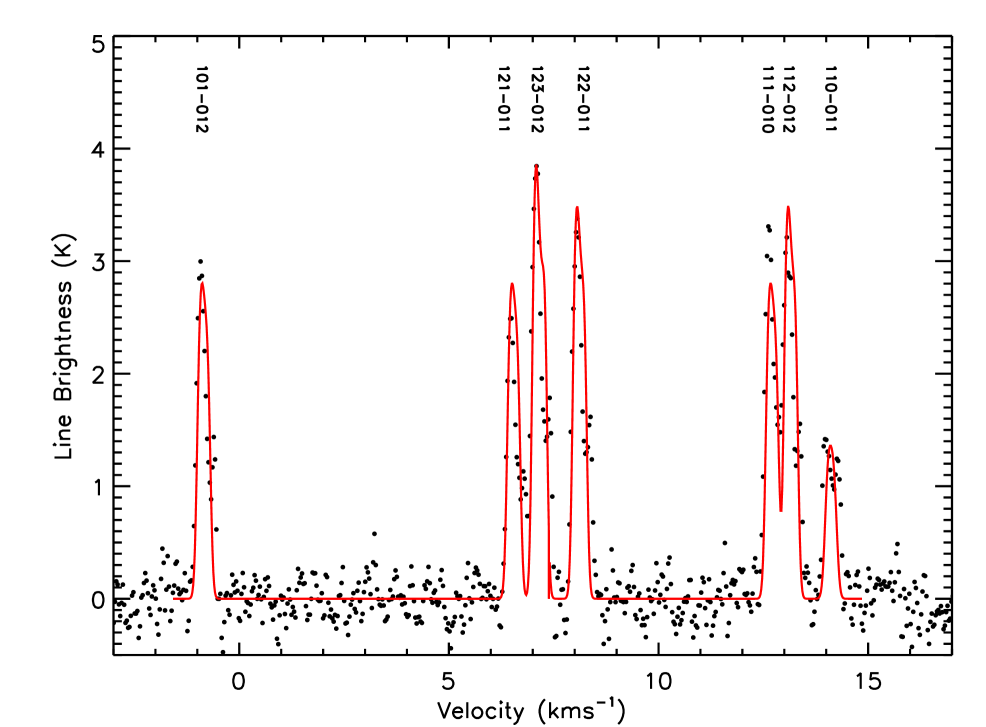
Figure 2: Observed N₂H⁺(1-0) spectrum of L1544 modeled with the HSE approximation. The dots show the observational data from Caselli et al. (1995). The line shows a model spectrum computed for a theoretical dark cloud (Keto & Caselli 2009) using our 3D radiative transfer code, MOLLIE, and the HSE approximation. In this approximation, the three hyperfine lines, 101–012, 121–011, and 111–010, necessarily have equal relative intensities. The velocity labeling includes the velocity of the L1544 cloud with respect to the Sun.

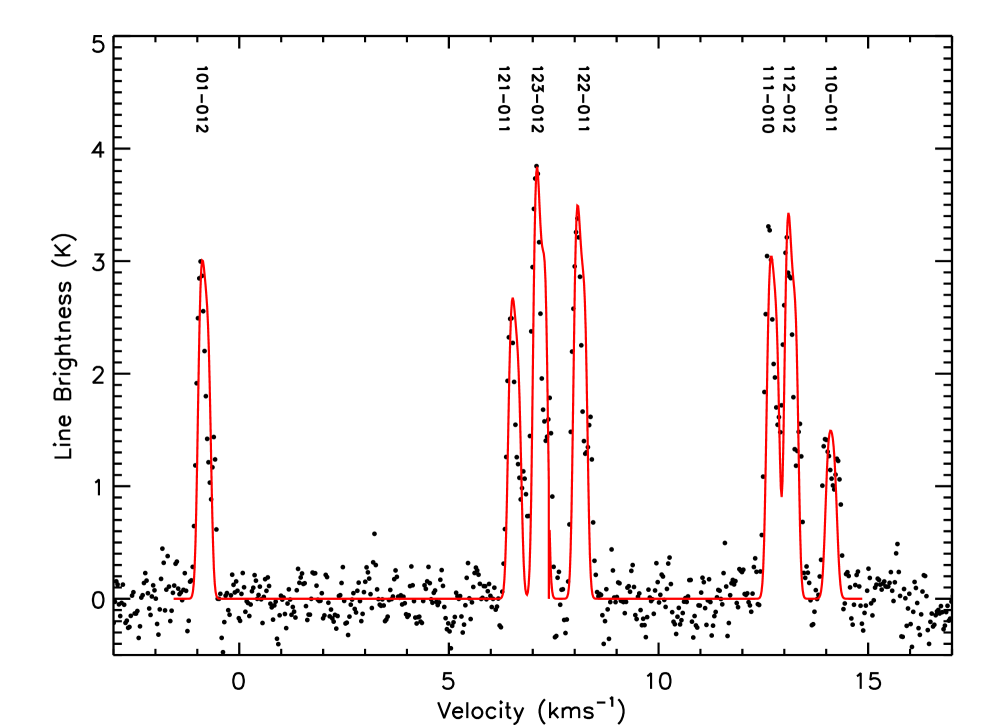
Figure 3: Observed N₂H⁺(1-0) spectrum of L1544 modeled with the proportional approximation. The same as figure 2 except that the model spectrum is computed with the proportional approximation, again using our radiative transfer code, MOLLIE. Non-LTE excitation results in unequal relative intensities for the 3 lines, 101–012, 121–011, and 111–010 and a better match to the data.

Figures 2 and 3 compare N₂H⁺(1-0) spectra of the same model cloud computed using the HSE and proportional approximations against the observed spectrum of L1544 (Caselli et al. 1999). The model is taken from Keto & Caselli (2009) and represents a slowly contracting gas cloud in radiative equilibrium with external starlight. L1544 is thought to be an example of this type of cloud. These spectra were made with our 3D radiative transfer code, MOLLIE (Keto 1990, Keto et al. 2004, Keto & Caselli 2009). The HSE approximation includes 8 rotational levels from $J=0$ to 7 and models the 7 $\Delta J=1$ rotational lines. The hyperfine splitting is included through the composite line profile function (equation 5). The proportional approximation includes 64 hyperfine levels in the rotational levels $J=0$ through 7 and all 280 hyperfine lines between those hyperfine levels. The two approximations result in different relative intensities for the hyperfine lines. The most evident are the different intensities of the three lines $JFF_{1}-J^{\prime}F^{\prime}F_{1}^{\prime}$ = 101–012, 121–011, and 111–010. In the LTE case, these three lines necessarily all have the same intensity whereas with non-LTE excitation, the 121–011 hyperfine is noticeably weaker and the 111–010 hyperfine is slightly brighter. The proportional approximation represents a better match to the data, yet for some purposes the HSE approximation may be good enough.

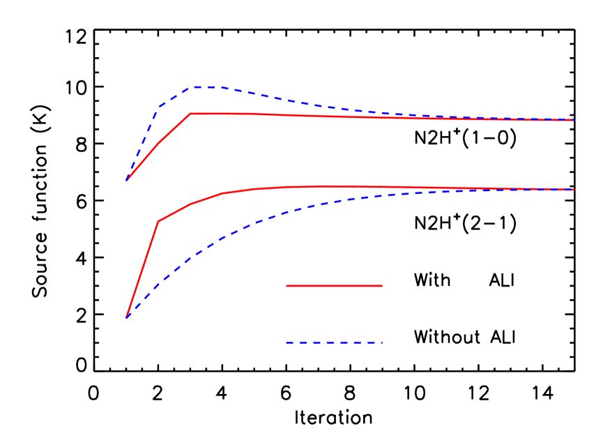
Figure 4: The convergence of the $\Lambda$ iteration with and without acceleration. The lines show the source function (equation 21) of the main (123–012) hyperfine line at the location of the center of the model cloud. The brightness of the spectrum in figure 3 is lower than the source function because of averaging lower brightness regions around the cloud center within the observing beam. This figure shows that in this calculation, the acceleration halves the required number of iterations.

Figure 4 compares the convergence of the $\Lambda$ iteration in the proportional approximation with the acceleration term (equation 25) and without ($\bar{\Lambda}_{JJ^{\prime}HH^{\prime}}=0$). In this example, the optical depth is less than 10 and the $\Lambda$ iteration converges quickly in both cases. However, convergence with the acceleration requires half the number of iterations. At higher optical depths, the acceleration would be considerably more significant.

5.2 Comparison of “exact” with “approximate” collision rates.

Because the collisional rates for the hyperfine transitions of N₂H⁺ have recently been calculated (Daniel et al. 2006), we can compare the spectra computed with these rates and with the approximate collision rates of the proportional approximation. In this comparison, we again use the same model for both calculations, changing only the collisional rate coefficients. In this example, we consider a uniform plane-parallel model of a molecular cloud with a size of $4.11\times 10^{17}$ cm, density of $10^{5}$ cm^-3, temperature of 8.9 K, abundance of N₂H⁺ relative to H₂ of $3\times 10^{-10}$, microturbulent line broadening of 0.06 kms^-1, and a constant and zero velocity field. The exterior boundary condition assumes radiation at the 2.728 K background. These parameters were chosen to reproduce the N₂H⁺(1-0) hyperfine line ratios in the observations of L1512 (Caselli et al 1995). This calculation includes 37 hyperfine levels in the rotational levels $J=0$ through 4 and all 145 hyperfine lines between those hyperfine levels. The fit to the data is shown in figure 5. The data for L1512 show the same pattern of non-LTE hyperfine line ratios as for L1544 with the 121-011 hyperfine noticeably lower than the 101–012 and 111–010 lines.

Figure 6 compares the spectra computed from the approximate and “exact” collision rates. Spectra for the 3 lowest rotational transitions of N₂H⁺, (1-0), (2-1), and (3-2) are shown along with the difference between the two. The difference is less than one percent of the line strength. For most observations of radio frequency molecular lines from dark clouds, this difference would be below the typical signal-to-noise ratio. Based on this example, the proportional approximation is adequate for N₂H⁺ and could be useful for other molecules with unknown hyperfine collision rates.

6 Conclusions

The modeling of molecular spectra with hyperfine splitting by ALI or Monte Carlo methods has been hampered by the lack of collisional rate coefficients for the hyperfine transitions. Two approximations previously suggested, the approximation of hyperfine statistical equilibrium (HSE) and the proportional approximation, both provide satisfactory results in tests modeling N₂H⁺ spectra. The HSE approximation, based on a modified line profile function, is simpler to implement, faster to compute, and models the non-LTE distribution in the rotational levels but cannot model non-LTE distributions of the hyperfine levels themselves. The proportional approximation uses easily computed approximate hyperfine collision rates, and is able to model non-LTE hyperfine emission with an accuracy comparable to calculations using the exact hyperfine collision rates. These results suggest that these two methods could also be useful for other molecules with hyperfine splitting.

7 Appendix

7.1 Statistical Weights for N₂H⁺

The hyperfine levels of N₂H⁺ are described by three angular momentum quantum numbers, $J$, $F_{1}$, and $F$. The first of these, $J$, refers to the molecular rotation, which is coupled to the spins of the outer and inner nitrogen nuclei $I_{1}=1$ and $I_{2}=1$, respectively. The coupling proceeds in two steps, first ${\hat{F}}_{1}={\hat{J}}+{\hat{I}}_{1}$, then ${\hat{F}}={\hat{F}}_{1}+{\hat{I}}_{2}$, which provide the remaining two quantum numbers $F_{1}$ and $F$. The statistical weight of a hyperfine level $JF_{1}F$ is given by $2F+1$, while the total statistical weight of rotational level $J$ is $g_{J}=(2I_{1}+1)(2I_{2}+1)(2J+1)=9(2J+1)$.

In LTE, the population in hyperfine state $H=F_{1}F$ relative to the total population in rotational level $J$ is,

$$n_{JH}=n_{J}\bigg{(}{{2F+1}\over{9(2J+1)}}\bigg{)}$$ (29)

The statistical degeneracies of the hyperfine states belonging to each J level sum to the total statistical degeneracy of the J level.

$$\sum_{F}(2F+1)=9(2J+1)$$ (30)

8 Einstein A for N₂H⁺

The Einstein A of a transition between rotational levels $JJ^{\prime}$ is a weighted sum of all the Einstein A’s between the individual hyperfine states of each $J$ and $J^{\prime}$ level, If the level populations are in LTE, indicated by an asterisk,

$$n^{*}_{J}A_{JJ^{\prime}}=\sum_{HH^{\prime}}n^{*}_{JH}A_{JHJ^{\prime}H^{\prime}}R_{JHJ^{\prime}H^{\prime}}$$ (31)

If the relative intensities $R_{JHJ^{\prime}H^{\prime}}$ are normalized so that,

$$\sum_{HH}R_{JHJ^{\prime}H^{\prime}}=1$$ (32)

then

$$A_{JHJ^{\prime}H^{\prime}}={{9(2J+1)}\over{{2F+1}A_{JJ^{\prime}}R_{JHJ^{\prime}H^{\prime}}}}$$ (33)

For any rotational transition,

$$A_{JJ^{\prime}}={{64\pi^{4}\nu^{3}}\over{3hc^{3}}}|\mu_{ij}|^{2}$$ (34)

The average dipole moment, $|\mu_{ij}|^{2}$, for a rotational transition of a linear molecule is (Townes & Schawlow, equation 1-76, pg 23),

$$|\mu_{ij}|^{2}=\mu^{2}{{J}\over{2J+1}}$$ (35)

if J is the initial state and the upper state. In this case, $J\rightarrow J-1$. As in Townes and Schalow, $|\mu_{ij}|^{2}$ can also be defined in ”absorption”, $J\rightarrow J+1$, with $J$ as the initial and lower state, or in ”emission”, $J+1\rightarrow J$, with J as the final and lower state. In these two alternate definitions, $|\mu_{ij}|^{2}=\mu^{2}(J+1)/(2J+1)$ and $|\mu_{ij}|^{2}=\mu^{2}(J+1)/(2J+3)$ respectively.

With our definitions for $J$ and $R$, the Einstein A for a hyperfine transition is,

$$A_{JHJ^{\prime}H^{\prime}}={{9(2J+1)}\over{2F+1}}\bigg{[}{{64\pi^{4}\nu^{3}}\over{3hc^{3}}}\bigg{]}\mu^{2}{{J}\over{2J+1}}R_{JHJ^{\prime}H^{\prime}}$$ (36)

The Einstein A’s for the individual hyperfine transitions sum to,

$$\sum_{HH^{\prime}}{{2F+1}\over{9(2J+1)}}A_{JHJ^{\prime}H^{\prime}}=A_{JJ^{\prime}}$$ (37)

8.1 Collision rates for N₂H⁺

For N₂H⁺ the approximate collisional rate coefficients in the proportional approximation are,

$$\tilde{C}_{JF_{1}FJ^{\prime}F_{1}^{\prime}F^{\prime}}={2F^{\prime}+1\over g(J^{\prime})}C_{JJ^{\prime}}.$$ (38)

$$C_{JJ^{\prime}}=\sum_{F_{1}FF_{1}^{\prime}F^{\prime}}{2F+1\over g(J)}\tilde{C}_{JF_{1}FJ^{\prime}F_{1}^{\prime}F^{\prime}},$$ (39)

8.2 Frequencies and relative intensities of N₂H⁺hyperfine lines

The frequencies and relative intensities of the hyperfine lines of N₂H⁺ are most accurately calculated by numerical methods (Pickett 1991). Dr. Luca Dore at the University of Bologna kindly supplied these data. Table 1 shows the results for $JJ^{\prime}=1-0$ rotational transition. This line is split into 16 hyperfine transitions at 7 different frequencies to produce 7 hyperfine lines. Tables 2 and 3 contain additional information on all the hyperfine states and transitions for J levels 1 through 7. Data on the frequencies and relative intensities of the hyperfine transitions of N₂D⁺ are available in Gerin et al. (2001) and Dore et al. (2004).

Table 1: N₂H⁺Hyperfine Line Data for $J=1\rightarrow 0$

Line label	Frequency	Line Strength	Components	Component Strength
$JF_{1}F$–$J^{\prime}F^{\prime}F_{1}^{\prime}$	(MHz)	$S_{F_{1}F-F^{\prime}F_{1}^{\prime}}$	$JF_{1}F\rightarrow J^{\prime}F_{1}^{\prime}F^{\prime}$	$S_{JF_{1}F\rightarrow J^{\prime}F_{1}^{\prime}F^{\prime}}$
110–011	93171.6086	0.33334	$110\rightarrow 011$	0.33334
112–012	93171.9054	1.66667	$112\rightarrow 012$	1.40832
			$112\rightarrow 011$	0.25837
111–010	93172.0403	1.00000	$111\rightarrow 011$	0.11979
			$111\rightarrow 012$	0.37225
			$111\rightarrow 010$	0.50797
122–011	93173.4675	1.66667	$122\rightarrow 011$	1.40830
			$122\rightarrow 012$	0.25836
123–012	93173.7643	2.33333	$123\rightarrow 012$	2.33333
121–011	93173.9546	1.00000	$121\rightarrow 012$	0.03938
			$121\rightarrow 011$	0.64660
			$121\rightarrow 010$	0.31402
101–012	93176.2527	1.00000	$101\rightarrow 010$	0.17802
			$101\rightarrow 011$	0.23361
			$101\rightarrow 012$	0.58836

Figure 1: Extrapolation to $\Delta J=0$ by empirical fit of the known inelastic collisional rates. The upper six panels show the collisional rates $C_{JJ^{\prime}}$ for six different $\Delta J$ written as $K_{JJ^{\prime}}=\log\bigg{(}{{C_{JJ^{\prime}}}\over{1+\Delta E_{JJ^{\prime}}/kT}}{{g_{J}}\over{g_{J^{\prime}}}}\times 10^{10}\bigg{)}$ versus $(\Delta E/kT)^{1/2}$. Equation 28 is linear in this choice of coordinate axes and is plotted for the six different $a(\Delta J)$ and $b(\Delta J)$ in each of the six panels. The lower two panels show these 6 lines for $\Delta J=1$ through 6 and the extrapolation to $\Delta J=0$.

Figure 5: Observed N₂H⁺(1-0) spectrum of L1512 modeled using the “exact” hyperfine collisional rates. The observational data (dots) are from Caselli et al. (1995). The line shows the model spectrum computed using the “exact” hyperfine collisional rates from Daniel et al. (2006). The model spectrum is computed with a 1-dimensional plane-parallel radiative transfer program.

Figure 6: Comparison of model N₂H⁺ spectra using approximate versus “exact” collisional rates. These 3 panels compare model spectra for the $\Delta J=1-0$, 2–1, and 3–2 rotational transitions. The upper portion of each panel shows both the spectrum, $\tilde{T}$, computed with the approximate hyperfine collisional rates of the proportional approximation and the spectrum $T$ computed with the “exact” rates from Daniel et al. (2006). The two spectra are so close as to be indistiguishable. The difference between the two spectra, $\Delta T$, multiplied by 1000, is plotted in the lower portion of each panel.

Table 2: N₂H⁺Hyperfine Level Data

Level	Energy	Statistical Weight	J	F1	F
	cm-1
1	0.0000	5.0	0	1	2
2	0.0000	3.0	0	1	1
3	0.0000	1.0	0	1	0
4	3.1057	1.0	1	1	0
5	3.1057	5.0	1	1	2
6	3.1057	3.0	1	1	1
7	3.1058	5.0	1	2	2
8	3.1058	7.0	1	2	3
9	3.1058	3.0	1	2	1
10	3.1059	3.0	1	0	1
11	9.3172	5.0	2	2	2
12	9.3172	7.0	2	2	3
13	9.3172	3.0	2	2	1
14	9.3173	7.0	2	3	3
15	9.3173	9.0	2	3	4
16	9.3173	5.0	2	3	2
17	9.3173	3.0	2	1	1
18	9.3173	5.0	2	1	2
19	9.3173	1.0	2	1	0
20	18.6343	7.0	3	3	3
21	18.6343	9.0	3	3	4
22	18.6343	5.0	3	3	2
23	18.6343	9.0	3	4	4
24	18.6343	11.0	3	4	5
25	18.6344	7.0	3	4	3
26	18.6344	5.0	3	2	2
27	18.6344	7.0	3	2	3
28	18.6344	3.0	3	2	1
29	31.0567	9.0	4	4	4
30	31.0567	11.0	4	4	5
31	31.0567	7.0	4	4	3
32	31.0568	11.0	4	5	5
33	31.0568	7.0	4	3	3
34	31.0568	13.0	4	5	6
35	31.0568	9.0	4	5	4
36	31.0568	9.0	4	3	4
37	31.0568	5.0	4	3	2
38	46.5842	11.0	5	5	5
39	46.5842	9.0	5	5	4
40	46.5842	13.0	5	5	6
41	46.5842	13.0	5	6	6
42	46.5843	9.0	5	4	4
43	46.5843	11.0	5	6	5
44	46.5843	15.0	5	6	7
45	46.5843	11.0	5	4	5
46	46.5843	7.0	5	4	3
47	65.2164	13.0	6	6	6
48	65.2164	11.0	6	6	5
49	65.2164	15.0	6	6	7
50	65.2165	15.0	6	7	7
51	65.2165	11.0	6	5	5
52	65.2165	13.0	6	7	6
53	65.2165	17.0	6	7	8
54	65.2165	9.0	6	5	4
55	65.2165	13.0	6	5	6
56	86.9529	15.0	7	7	7
57	86.9529	13.0	7	7	6
58	86.9529	17.0	7	7	8
59	86.9530	17.0	7	8	8
60	86.9530	13.0	7	6	6
61	86.9530	15.0	7	8	7
62	86.9530	19.0	7	8	9
63	86.9530	11.0	7	6	5
64	86.9530	15.0	7	6	7

Table 3: N₂H⁺Hyperfine Level Data

Transition	Upper State	Lower State	Einstein A	Frequency	Relative Intensity
			s-1	GHz
1	4	2	3.6202E-05	93.1716086	3.703754E-02
2	5	2	5.6121E-06	93.1719054	2.870743E-02
3	5	1	3.0591E-05	93.1719054	1.564799E-01
4	6	3	1.8390E-05	93.1720403	5.644098E-02
5	6	2	4.3366E-06	93.1720403	1.330977E-02
6	6	1	1.3476E-05	93.1720403	4.136132E-02
7	7	2	3.0592E-05	93.1734675	1.564777E-01
8	7	1	5.6123E-06	93.1734675	2.870710E-02
9	8	1	3.6204E-05	93.1737643	2.592588E-01
10	9	2	2.3410E-05	93.1739546	7.184409E-02
11	9	1	1.4259E-06	93.1739546	4.375910E-03
12	9	3	1.1369E-05	93.1739547	3.489065E-02
13	10	3	6.4454E-06	93.1762527	1.977944E-02
14	10	2	8.4583E-06	93.1762527	2.595644E-02
15	10	1	2.1303E-05	93.1762527	6.537287E-02
16	11	10	2.7992E-08	186.3401767	4.474821E-06
17	13	10	3.0605E-07	186.3404984	2.935571E-05
18	16	10	1.5304E-06	186.3424717	2.446410E-04
19	11	9	1.1350E-05	186.3424747	1.814322E-03
20	11	8	2.6929E-05	186.3426651	4.304765E-03
21	13	9	2.0609E-04	186.3427964	1.976683E-02
22	12	8	1.7449E-04	186.3429204	3.905121E-02
23	11	7	6.8980E-05	186.3429618	1.102677E-02
24	17	10	3.7407E-04	186.3430541	3.587865E-02
25	12	7	2.1961E-05	186.3432171	4.914732E-03
26	18	10	3.8710E-04	186.3432658	6.187998E-02
27	13	7	3.3348E-05	186.3432835	3.198466E-03
28	19	10	4.0897E-04	186.3435179	1.307500E-02
29	11	6	4.1510E-04	186.3443890	6.635387E-02
30	14	8	5.7200E-05	186.3444527	1.280094E-02
31	11	5	1.7271E-04	186.3445240	2.760721E-02
32	13	6	1.2012E-04	186.3447107	1.152066E-02
33	14	7	6.3721E-04	186.3447494	1.426027E-01
34	16	9	5.5131E-04	186.3447698	8.812664E-02
35	12	5	4.9863E-04	186.3447793	1.115900E-01
36	13	5	1.0558E-05	186.3448457	1.012611E-03
37	15	8	6.9509E-04	186.3448501	1.999999E-01
38	16	8	3.6017E-06	186.3449601	5.757276E-04
39	13	4	3.2467E-04	186.3451424	3.113882E-02
40	16	7	1.3303E-04	186.3452569	2.126449E-02
41	17	9	1.7064E-06	186.3453521	1.636638E-04
42	18	9	2.2819E-06	186.3455638	3.647582E-04
43	18	8	1.5809E-05	186.3457542	2.527066E-03
44	19	9	2.7376E-05	186.3458160	8.752108E-04
45	17	7	9.9051E-06	186.3458392	9.499830E-04
46	18	7	7.6819E-06	186.3460509	1.227927E-03
47	14	5	6.7821E-07	186.3463116	1.517738E-04
48	16	6	4.2661E-06	186.3466841	6.819109E-04
49	16	5	1.3617E-06	186.3468190	2.176538E-04
50	17	6	1.0864E-04	186.3472664	1.041905E-02
51	17	5	1.3927E-04	186.3474014	1.335727E-02
52	18	6	8.6729E-05	186.3474781	1.386316E-02
53	18	5	1.9549E-04	186.3476131	3.124782E-02
54	17	4	6.1497E-05	186.3476981	5.897943E-03
55	19	6	2.5875E-04	186.3477303	8.271997E-03
56	20	18	3.4882E-07	279.5085967	1.028071E-05
57	22	18	1.8603E-06	279.5090304	3.916298E-05
58	22	17	3.2591E-06	279.5092421	6.861077E-05
59	20	16	1.6539E-05	279.5093908	4.874558E-04
60	20	15	3.3819E-05	279.5095008	9.967375E-04
61	22	16	4.6438E-04	279.5098245	9.776190E-03
62	21	15	4.3854E-04	279.5098785	1.661797E-02
63	20	14	2.4117E-04	279.5098982	7.107855E-03
64	21	14	3.6220E-05	279.5102760	1.372515E-03
65	22	14	3.7711E-05	279.5103319	7.938893E-04
66	25	18	2.4184E-06	279.5110156	7.127707E-05
67	26	18	7.3142E-04	279.5111328	1.539760E-02
68	26	17	2.2761E-03	279.5113445	4.791484E-02
69	28	19	1.7593E-03	279.5113847	2.222227E-02
70	23	15	1.8979E-04	279.5114140	7.191670E-03
71	20	12	4.7599E-04	279.5114305	1.402838E-02
72	27	18	3.2067E-03	279.5115089	9.451005E-02
73	28	18	8.5742E-05	279.5116369	1.082997E-03
74	20	11	3.0022E-03	279.5116858	8.848041E-02
75	22	13	2.8961E-03	279.5117978	6.096633E-02
76	21	12	3.2953E-03	279.5118083	1.248667E-01
77	25	16	3.4109E-03	279.5118097	1.005275E-01
78	23	14	3.5787E-03	279.5118114	1.356067E-01
79	28	17	1.4792E-03	279.5118486	1.868338E-02
80	24	15	3.7700E-03	279.5118621	1.746030E-01
81	22	12	1.3014E-05	279.5118642	2.739705E-04
82	25	15	5.2440E-06	279.5119197	1.545508E-04
83	26	16	6.5715E-10	279.5119269	1.383404E-08
84	22	11	3.5375E-04	279.5121195	7.446892E-03
85	27	16	2.4855E-06	279.5123029	7.325300E-05
86	25	14	3.4636E-04	279.5123171	1.020782E-02
87	27	15	1.4795E-05	279.5124130	4.360447E-04
88	28	16	1.9535E-05	279.5124309	2.467483E-04
89	26	14	1.2137E-05	279.5124343	2.555042E-04
90	27	14	7.1706E-06	279.5128104	2.113294E-04
91	23	12	1.5528E-06	279.5133437	5.884003E-05
92	25	12	2.0645E-06	279.5138494	6.084373E-05
93	26	13	1.0267E-04	279.5139002	2.161342E-03
94	26	12	1.0470E-04	279.5139666	2.203971E-03
95	25	11	3.0217E-06	279.5141047	8.905449E-05
96	26	11	5.4306E-04	279.5142219	1.143186E-02
97	27	12	4.7716E-04	279.5143427	1.406264E-02
98	28	13	2.8018E-04	279.5144042	3.538813E-03
99	27	11	6.1682E-05	279.5145980	1.817842E-03
100	28	11	1.4606E-04	279.5147260	1.844849E-03
101	29	27	7.4736E-07	372.6695840	6.721026E-06
102	31	27	2.3618E-06	372.6700461	1.651944E-05
103	29	25	1.9884E-05	372.6700772	1.788133E-04
104	29	24	3.7991E-05	372.6701349	3.416527E-04
105	31	26	4.8732E-06	372.6704221	3.408610E-05
106	31	25	8.3318E-04	372.6705393	5.827693E-03
107	30	24	8.1806E-04	372.6705729	8.991692E-03
108	29	23	5.2594E-04	372.6705829	4.729776E-03
109	30	23	4.6530E-05	372.6710209	5.114248E-04
110	31	23	4.0936E-05	372.6710450	2.863249E-04
111	33	27	1.1668E-03	372.6719768	8.161053E-03
112	35	27	2.4924E-06	372.6720656	2.241399E-05
113	29	21	8.9202E-04	372.6721184	8.021803E-03
114	32	24	4.1747E-04	372.6721184	4.588582E-03
115	37	28	9.5314E-03	372.6723529	4.761915E-02
116	33	26	9.9301E-03	372.6723529	6.945553E-02
117	36	27	1.1416E-02	372.6724208	1.026622E-01
118	33	25	1.5072E-07	372.6724701	1.054191E-06
119	37	27	4.8486E-05	372.6724809	2.422388E-04
120	29	20	1.0879E-02	372.6724961	9.783247E-02
121	31	22	1.0756E-02	372.6725246	7.523414E-02
122	30	21	1.1491E-02	372.6725564	1.262994E-01
123	35	25	1.1675E-02	372.6725589	1.049958E-01
124	32	23	1.1936E-02	372.6725665	1.311891E-01
125	31	21	1.3873E-05	372.6725805	9.703108E-05
126	34	24	1.2356E-02	372.6725984	1.604938E-01
127	35	24	6.4340E-06	372.6726165	5.785998E-05
128	37	26	1.9766E-03	372.6728570	9.875358E-03
129	36	25	2.4223E-06	372.6729140	2.178349E-05
130	31	20	7.0399E-04	372.6729582	4.924026E-03
131	36	24	1.4411E-05	372.6729717	1.295961E-04
132	37	25	1.7187E-05	372.6729742	8.586414E-05
133	33	23	1.2905E-05	372.6729758	9.026414E-05
134	35	23	6.6612E-04	372.6730646	5.990276E-03
135	36	23	6.6651E-06	372.6734197	5.993804E-05
136	32	21	2.2510E-06	372.6741019	2.474133E-05
137	33	22	1.1135E-04	372.6744553	7.788442E-04
138	33	21	8.9884E-05	372.6745112	6.286748E-04
139	35	21	2.3130E-06	372.6746001	2.080038E-05
140	33	20	1.0443E-03	372.6748890	7.304192E-03
141	36	21	8.6344E-04	372.6749552	7.764664E-03
142	37	22	6.7097E-04	372.6749594	3.352110E-03
143	35	20	2.6493E-06	372.6749778	2.382391E-05
144	36	20	5.2589E-05	372.6753329	4.729110E-04
145	37	20	1.1084E-04	372.6753931	5.537304E-04
146	38	36	1.0095E-06	465.8220241	3.636243E-06
147	38	35	2.2212E-05	465.8223792	8.000664E-05
148	38	34	4.0780E-05	465.8223974	1.468922E-04
149	39	36	2.4047E-06	465.8224922	7.086887E-06
150	39	35	1.3109E-03	465.8228473	3.863332E-03
151	40	34	1.3104E-03	465.8228727	5.578354E-03
152	38	32	9.2218E-04	465.8228774	3.321732E-03
153	39	33	5.5265E-06	465.8229362	1.628706E-05
154	39	32	4.3197E-05	465.8233455	1.273055E-04
155	40	32	5.3971E-05	465.8233527	2.297488E-04
156	42	36	1.7098E-03	465.8243347	5.038865E-03
157	38	30	1.4184E-03	465.8244229	5.109088E-03
158	41	34	7.4606E-04	465.8244293	3.175888E-03
159	43	36	2.3110E-06	465.8245447	8.324153E-06
160	42	35	2.8176E-07	465.8246899	8.303576E-07
161	46	37	2.6930E-02	465.8247706	6.172843E-02
162	42	33	2.7294E-02	465.8247787	8.043820E-02
163	45	36	2.9420E-02	465.8248172	1.059706E-01
164	46	36	3.5978E-05	465.8248307	8.246709E-05
165	38	29	2.8443E-02	465.8248609	1.024497E-01
166	39	31	2.8303E-02	465.8248669	8.341198E-02
167	39	30	1.4222E-05	465.8248910	4.191243E-05
168	40	30	2.9483E-02	465.8248982	1.255051E-01
169	43	35	2.9740E-02	465.8248999	1.071222E-01
170	41	32	3.0098E-02	465.8249092	1.281255E-01
171	43	34	7.3139E-06	465.8249180	2.634444E-05
172	44	34	3.0847E-02	465.8249325	1.515151E-01
173	45	35	2.1966E-06	465.8251724	7.912265E-06
174	46	35	1.6064E-05	465.8251859	3.682110E-05
175	42	32	1.3213E-05	465.8251880	3.894043E-05
176	45	34	1.4224E-05	465.8251905	5.123376E-05
177	46	33	2.6025E-03	465.8252747	5.965332E-03
178	39	29	1.1677E-03	465.8253290	3.441266E-03
179	43	32	1.0930E-03	465.8253980	3.937066E-03
180	45	32	6.1763E-06	465.8256705	2.224666E-05
181	41	30	2.7699E-06	465.8264548	1.179111E-05
182	42	31	1.1238E-04	465.8267094	3.311910E-04
183	42	30	8.1702E-05	465.8267335	2.407777E-04
184	43	30	2.3071E-06	465.8269436	8.309887E-06
185	42	29	1.6357E-03	465.8271716	4.820332E-03
186	46	31	1.1677E-03	465.8272054	2.676621E-03
187	45	30	1.3564E-03	465.8272160	4.885510E-03
188	43	29	2.4536E-06	465.8273816	8.837820E-06
189	45	29	4.8153E-05	465.8276541	1.734440E-04
190	46	29	9.4852E-05	465.8276675	2.174124E-04
191	47	45	1.1935E-06	558.9639040	2.042074E-06
192	47	44	4.2772E-05	558.9641620	7.318242E-05
193	47	43	2.3919E-05	558.9641765	4.092575E-05
194	48	45	2.2321E-06	558.9643698	3.231556E-06
195	48	43	1.8969E-03	558.9646423	2.746241E-03
196	49	44	1.9142E-03	558.9646639	3.779000E-03
197	47	41	1.4288E-03	558.9646653	2.444574E-03
198	48	42	5.8004E-06	558.9648524	8.397519E-06
199	48	41	4.4831E-05	558.9651311	6.490390E-05
200	49	41	5.9499E-05	558.9651672	1.174626E-04
201	51	45	2.3611E-03	558.9661589	3.418204E-03
202	47	40	2.0547E-03	558.9662218	3.515574E-03
203	50	44	1.1782E-03	558.9662309	2.326019E-03
204	51	43	2.9343E-07	558.9664314	4.248112E-07
205	52	45	1.9404E-06	558.9664518	3.319926E-06
206	54	46	5.9693E-02	558.9666312	7.070705E-02
207	51	42	6.0051E-02	558.9666414	8.693816E-02
208	54	45	2.9943E-05	558.9666447	3.546815E-05
209	55	45	6.2917E-02	558.9666677	1.076489E-01
210	48	40	1.4375E-05	558.9666877	2.081056E-05
211	48	39	6.1233E-02	558.9666949	8.864964E-02
212	47	38	6.1389E-02	558.9666971	1.050348E-01
213	52	44	7.9800E-06	558.9667098	1.365354E-05
214	49	40	6.2967E-02	558.9667237	1.243087E-01
215	52	43	6.3299E-02	558.9667243	1.083022E-01
216	50	41	6.3759E-02	558.9667342	1.258728E-01
217	53	44	6.4941E-02	558.9667527	1.452991E-01
218	54	43	1.5398E-05	558.9669172	1.823909E-05
219	51	41	1.3346E-05	558.9669202	1.932111E-05
220	55	44	1.4124E-05	558.9669258	2.416574E-05
221	55	43	1.8145E-06	558.9669402	3.104611E-06
222	54	42	3.3454E-03	558.9671272	3.962630E-03
223	48	38	1.7433E-03	558.9671630	2.523815E-03
224	52	41	1.6274E-03	558.9672131	2.784334E-03
225	55	41	5.6603E-06	558.9674290	9.684427E-06
226	50	40	3.1583E-06	558.9682907	6.234927E-06
227	51	40	7.6533E-05	558.9684767	1.107989E-04
228	51	39	1.1150E-04	558.9684840	1.614180E-04
229	52	40	2.1317E-06	558.9687696	3.647241E-06
230	51	38	2.3270E-03	558.9689521	3.368852E-03
231	54	39	1.7712E-03	558.9689698	2.097963E-03
232	55	40	1.9564E-03	558.9689855	3.347352E-03
233	52	38	2.3211E-06	558.9692449	3.971297E-06
234	54	38	8.5854E-05	558.9694378	1.016933E-04
235	55	38	4.5549E-05	558.9694608	7.793205E-05
236	56	55	1.3333E-06	652.0931420	1.217987E-06
237	56	53	4.4263E-05	652.0933151	4.043571E-05
238	56	52	2.5221E-05	652.0933579	2.304032E-05
239	57	55	1.9271E-06	652.0936022	1.525759E-06
240	57	52	2.5909E-03	652.0938182	2.051286E-03
241	56	50	2.0449E-03	652.0938368	1.868063E-03
242	58	53	2.6286E-03	652.0938378	2.721444E-03
243	57	51	5.9171E-06	652.0941110	4.684698E-06
244	57	50	4.6055E-05	652.0942971	3.646270E-05
245	58	50	6.3735E-05	652.0943595	6.598698E-05
246	60	55	3.1204E-03	652.0953552	2.470444E-03
247	56	49	2.8009E-03	652.0954039	2.558698E-03
248	59	53	1.7153E-03	652.0954144	1.775921E-03
249	60	52	2.1814E-07	652.0955711	1.727079E-07
250	61	55	1.3855E-06	652.0957103	1.265668E-06
251	63	55	2.6453E-05	652.0958303	1.772095E-05
252	63	54	1.1483E-01	652.0958533	7.692302E-02
253	60	51	1.1519E-01	652.0958640	9.119825E-02
254	57	49	1.4442E-05	652.0958641	1.143360E-05
255	61	53	8.4931E-06	652.0958833	7.758603E-06
256	64	55	1.1890E-01	652.0958841	1.086189E-01
257	57	48	1.1654E-01	652.0959001	9.226698E-02
258	56	47	1.1671E-01	652.0959058	1.066197E-01
259	61	52	1.1935E-01	652.0959262	1.090254E-01
260	58	49	1.1894E-01	652.0959266	1.231386E-01
261	59	50	1.1991E-01	652.0959362	1.241465E-01
262	62	53	1.2163E-01	652.0959520	1.407408E-01
263	63	52	1.4947E-05	652.0960462	1.001292E-05
264	60	50	1.3402E-05	652.0960500	1.061060E-05
265	64	53	1.4074E-05	652.0960571	1.285665E-05
266	64	52	1.2687E-06	652.0961000	1.158940E-06
267	63	51	4.2008E-03	652.0963391	2.814175E-03
268	57	47	2.4300E-03	652.0963660	1.923873E-03
269	61	50	2.2692E-03	652.0964051	2.072937E-03
270	64	50	5.0682E-06	652.0965789	4.629841E-06
271	59	49	3.4558E-06	652.0975032	3.577825E-06
272	60	49	7.2981E-05	652.0976170	5.777952E-05
273	60	48	1.1019E-04	652.0976530	8.723968E-05
274	61	49	1.8230E-06	652.0979721	1.665302E-06
275	60	47	3.1221E-03	652.0981189	2.471810E-03
276	63	48	2.4822E-03	652.0981281	1.662810E-03
277	64	49	2.6639E-03	652.0981459	2.433460E-03
278	61	47	2.2168E-06	652.0984740	2.025063E-06
279	63	47	8.0111E-05	652.0985940	5.366651E-05
280	64	47	4.3847E-05	652.0986478	4.005444E-05

References

- Caselli, Myers, & Thaddeus (1995) Caselli, P., Myers, P., & Thaddeus, P. 1995, ApJ, 455, L77
- Caselli et al. (1999) Caselli, P., Walmsley, C., Tafalla, M., Dore, L., & Myers, P. 1999, Ap Jl, 523, 165
- Daniel et al. (2005) Daniel, F., Dubernet, M.-L., Meuwly, M., Cernicharo, J., & Pagani, L. 2005, MNRAS, 363, 1083
- Daniel et al. (2006) Daniel, F.; Cernicharo, J.; Dubernet, M.-L., 2006, ApJ, 648, 461
- deJong, Dalgarno & Chu (1975) deJong, T., Dalgarno, A., Chu, S.-I., 1975, ApJ, 199, 69
- Dore et al. (2004) Dore, L., Caselli, P., Beninati, S., Bourke, T., Myers, P.C., & Cazzoli, G., 2004, AA, 413, 1177
- Flower (1999) Flower, D., 1999, MNRAS 305, 651
- Gerin et al. (2001) Gerin, M., Pearson, J.C., Roueff, E., Falgarone, E., & Phillips, T.G., 2001, ApJL, 551, L193
- Green & Chapman (1978) Green, S. & Chapman, S., 1978, 37, 169
- Guilloteau & Baudry (1981) Guilloteau, S., & Baudry, A. 1981, A&A, 97,213
- Keto (1990) Keto, E., 1990, ApJ, 355, 190
- Keto et al. (2004) Keto, E., Rybicki, G.B., Bergin, E.A., Plume, R., 2004, ApJ, 613,355
- Pickett (1991) Pickett, H. 1991, J Molec. Spectroscopy, 1999, 148, 371
- Rybicki & Hummer (1991) Rybicki, G.B., & Hummer, D. 1991, A&A, 245, 171
- Rybicki & Hummer (1992) Rybicki, G.B., & Hummer, D. 1992, A&A, 262, 209
- Tafalla et al. (2004) Tafalla, M., Myers, P., Caselli, P., Walmsley, M., 2004, A&A, 416, 191