Atmospheric turbulence in phase-referenced and wide-field interferometric images:

Phase referencing is a standard calibration procedure in radio interferometry. It allows to detect weak sources by using quasi-simultaneous observations of closeby sources acting as calibrators. Therefore, it is assumed that, for each antenna, the optical paths of the signals from both sources are similar. However, atmospheric turbulence may introduce strong differences in the optical paths of the signals and affect, or even waste, phase referencing for cases of relatively large calibrator-to-target separations and/or bad weather. The situation is similar in wide-field observations, since the random deformations of the images, mostly caused by atmospheric turbulence, have essentially the same origin as the random astrometric variations of phase-referenced sources with respect to the phase center of their calibrators. In this paper, we present the results of a Monte Carlo study of the astrometric precision and sensitivity of an interferometric array (a realization of the Square Kilometre Array, SKA) in phase-referenced and wide-field observations. These simulations can be extrapolated to other arrays by applying the corresponding corrections. We consider several effects from the turbulent atmosphere (i.e., ionosphere and wet component of the troposphere) and also from the antenna receivers. We study the changes in dynamic range and astrometric precision as a function of observing frequency, source separation, and strength of the turbulence. We find that, for frequencies between 1 and 10 GHz, it is possible to obtain images with high fidelity, although the atmosphere strongly limits the sensitivity of the instrument compared to the case with no atmosphere. Outside this frequency window, the dynamic range of the images and the accuracy of the source positions decrease. We also find that, even if a good model of the atmospheric turbulence (with an accuracy of 99%) is used in the imaging, residual effects from the turbulence can still limit the dynamic ranges of deep, high-contrast ($10^{5}-10^{6}$), images.

1 Introduction

It is well-known that ground-based astronomical observations are affected by the atmosphere. Changes in the atmospheric opacity produce a bias in the source flux density, while changes in the refraction index distort the shape of the electromagnetic frontwave of the source. Such a distortion translates into a deformation of the observed source structure and/or a variation of the relative positions of all sources observed in a given field. In the case of astronomical devices based on interferometry, atmospheric effects can be well modelled if the atmosphere above each element of the interferometer (hereafter, station) remains unchanged over the whole portion of the sky being observed. In such cases, the observed visibilities can be calibrated using station-based algorithms, which are relatively simple and computationally inexpensive (e.g. Readhead & Wilkinson Readhead1978 (1978)).

However, when the spatial variations of the atmosphere are significant within the observed portion of the sky, as it happens if there is atmospheric turbulence, the opacity and dispersive effects cannot be modeled as a single time-dependent station-based complex gain over the field of view. Unless more complicated calibration algorithms are used (e.g., van der Tol, Jeffs, & van der Veen vdT07 (2007)), the effect of these errors on the image are difficult to correct. In this paper, we report on a study of the effects that a turbulent atmosphere may introduce in interferometric observations. We focus our study on the effects produced by turbulence in the dynamic range and astrometric accuracy after a phase-referenced calibration between a strong (calibrator) source and a weak source, located a few degrees away. This study is numerically equivalent to the study of the deformation of a wide-field interferometric image at any point located at a given distance from the center of the field (i.e., the phase center of the image). In both cases, the phases introduced by the atmosphere in the signal of each antenna for the different pointing directions are the same, so the effects of the atmosphere in Fourier space (and therefore on the sky plane) will also be the same.

The results here reported are an extended version of those previously reported in the SKA memo by Martí-Vidal et al. (MartiVidal2009 (2009)). In the next section, we describe the details of the array distribution used, as well as the characteristics of the simulated observations. In Sect. 3, we describe how the noise from the atmosphere and the receivers was added to the visibilities and in Sect. 4 describe the procedures followed in our Monte Carlo analysis. In Sect. 5, we present the main results obtained; in Sect. 6, we summarize our conclusions.

2 Array geometry and sensitivity

We simulated an interferometric array similar to the planned station distribution of the Square Kilometre Array (SKA). We simulated a total of 200 stations distributed in the following way: 50% are randomly distributed within a circle of 5 km radius (inner core); 25% are distributed outside this circle up to a distance of 150 km (core), following 5 equiangular spiral arms; the remaining antennae are distributed following the same spiral arms, but up to a distance of 3000 km from the inner core. This array distribution is similar to that used in Vir Lal, Lobanov & Jiménez-Monferrer (VLJ09 (2009)). The curvature of the Earth surface was taken into account in our simulations. We show the resulting array distribution in Fig. 1. We also repeated all the simulations here reported, but subtracting a subset of 100 (randomly selected) stations from the array, to check the sensitivity of the main conclusions of this paper on different array distributions (see Appendix A). We also show in Fig. 1 the modified array after subtracting the 100 stations.

Figure 1: Array distribution used in our simulations (empty and filled squares). Axes are relative Longitude (horizontal axis) and Latitude (vertical axis) in km. Left, the whole array. Center, a zoom to the core. Right, a zoom to the inner core. The stations marked with empty squares were removed from the array in a second run of our simulations, to check the dependence of the results on different array distributions (see text).

2.1 Sensitivity and bandwidth

We simulated interferometric observations using 16 different frequencies, which span in logarithmic bins from 150 MHz to 24 GHz (this is the theoretical frequency window of the SKA). According to Jones (J04 (2004)), the maximum observing bandwidth of the SKA will be around 25% of the central observing frequency (up to a maximum bandwidth of 4 GHz for all frequencies above 16 GHz). This (maximum) frequency-dependent bandwidth translates in our simulations into a changing sensitivity of the SKA as a function of frequency.

The sensitivities of the simulated stations were also chosen to be similar to those of the SKA, which were taken from Jones (J04 (2004)). These values are set for an elevation of 45 degrees and differ from those given in Schilizzi et al. (SAC07 (2007)), but the use of the values given in Schilizzi et al. (SAC07 (2007)), instead, does not affect the main conclusions of this paper. We interpolated the sensitivities given in Table 1 of Jones (J04 (2004)) to the frequencies used in our simulations. In Fig. 2 we show the station sensitivities used.

Figure 2: Station sensitivities (i.e., effective areas over system temperatures) used in our simulations.

2.2 Source position

We set the target source coordinates at the zenith of the array center and the calibrator at an hour angle of 0 degrees, also with respect to the array center. This position of the sources minimizes the optical paths of the signals through the atmosphere (since both, source and calibrator, are at maximum elevations), thus enhancing the quality of the phase-referenced observations. The results given in this paper should be interpreted according to this issue.

If the source would be located far from the zenith, the mapping function of the tropospheric delay and the finite width of the ionosphere would increase the effect of turbulence on the phase-referenced visibilities of the target. Additionally, the uv coverage of the interferometer would have shorter projected baselines in declination, thus decreasing the synthesized resolution in declination. Therefore, we want to stress that setting the sources at maximum elevations is a key limiting factor of the simulations here reported, especially if they are to be compared to real observations.

3 Noise model

We simulated phase-referencing observations in the following way: we assumed that the calibrator source is sufficiently strong to allow for a perfect antenna-gain calibration at its location; we then determined the image of the target source by computing the differential antenna-gain errors expected at the target location. Therefore, under the effect of atmospheric turbulence, these results depend on the calibrator-to-target separation.

We implemented two kinds of atmospheric turbulence. The first turbulence was associated to the ionosphere (the free electron content, which introduces dispersion in the radiation) and the other turbulence was associated to the wet troposphere (the water vapour, close to the earth surface, which is in a state of no thermodynamic equilibrium). The effect of ionospheric turbulence on the signal phase varies as $\nu^{-1}$, affecting the low-frequency observations; the effect of the wet troposphere on the phase varies as $\nu$, affecting the high-frequency observations. The dry troposphere (which is more homogeneously distributed over each station than the wet troposphere) was not considered in our simulations, since it can be easily modeled and removed from the data to a level lower than the effects coming from the water vapor and the ionosphere. Models of the turbulence from the ionosphere and troposphere can be found in many publications (e.g., Thomson, Moran, & Swenson TMS91 (1991)). Here, it is suffice to say that this turbulence follows a Kolmogorov distribution. This distribution has a phase structure function given by

$$D_{\phi}(\theta)=\leavevmode\nobreak\ <\left(\Phi(\theta_{0})-\Phi(\theta_{0}+\theta)\right)^{2}>\leavevmode\nobreak\ \propto\leavevmode\nobreak\ \theta^{5/3}$$ (1)

where $\Phi(\theta_{0})$ is the phase added by the turbulent screen to the signal of a source located at $\theta_{0}$. The brackets $<...>$ represent averaging over all pointing directions located at a distance $\theta$ from the point at $\theta_{0}$. The Kolmogorov distribution is fractal-like, so both, ionosphere and wet troposphere, have essentially the same phase distribution, despite of a global scaling factor between them.

The global factors for both distributions (ionosphere and troposphere) were computed according to the typical values of ionospheric and tropospheric conditions. For the ionosphere, the Fried length (i.e., distance in the ionosphere for which the structure function rises to 1 rad²) was set to 3 km at 100 MHz. For the wet troposphere, we set the parameter $C^{2}_{n}L$ (i.e., the integral of the profile of $C^{2}_{n}$ along the zenith direction) to $10^{-11}$ m^1/3 (vid. Eq. 13.100 and Table 13.2 of Thomson, Moran, & Swenson TMS91 (1991)); this value translates into a Fried length of 3 km for a frequency of $\sim 22$ GHz. Since the Kolmogorov distribution is self-similar, it is possible to adapt the results here reported to any other atmospheric conditions (see Sect. 5.3), just accordingly scaling the source separation to the Fried length of the ionosphere (for low-frequency observations) or the wet troposphere (for high-frequency observations). We must notice that the self-similarity of the tropospheric turbulence does not hold for very large scales (the typical baseline lengths in VLBI observations), since there is a saturation in the power spectrum of the distribution (see, e.g., Thomson, Moran, & Swenson TMS91 (1991)). However, this is not important in our analysis, since we did not use the absolute phase of the signal coming from a given direction in the sky, but computed the differential effects at each station from two different (closeby) directions, which depend on short-scale turbulence. Therefore, the saturation of tropospheric turbulence at large scales does not affect our results.

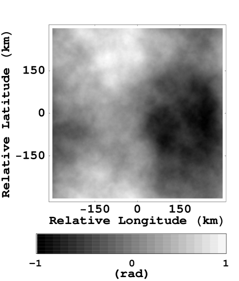
Figure 3: Example of a turbulent phase screen with Kolmogorov statistics. The grey scale shows variations of optical-path phases, normalized between $-1$ and 1 radians. The final values of the phases depend (given the self-similarity of the distribution) on a global factor related to the observing frequency and the ionospheric and/or wet tropospheric conditions.

We computed the differential effects from the turbulent atmosphere in two ways. For the antennas of the core (within the central 300 km) we generated synthetic phase screens for the ionosphere and troposphere. We show an example of one such screen in Fig. 3. We notice that this figure could represent either ionospheric or tropospheric turbulence in our modeling, just by scaling the screen by the corresponding factor. Two different screens were generated in each Monte Carlo simulation. The screen for simulating the ionosphere was put at a height of 300 km and the screen for simulating the troposphere was put at a height of 5 km. For the antennas out of the core, we computed the term $\Phi(\theta_{0})-\Phi(\theta_{0}+\theta)$ separately. We proceeded this way (i.e., we generated a phase screen only for the core antennas, thus without generating a much larger screen for the whole array), because the distances between stations out of the core are large enough to ensure that the cross-correlation of turbulence above different stations is negligible compared to the correlation between those on the calibrator and target source for the same station. This numerical strategy also speeded up our simulations.

It must be noticed that we did not introduce any time evolution of the turbulent phase screens in our simulations. Any evolution of the turbulence could dramatically affect the observations if the acquisition times were larger than the coherence time of the signal, which depends on the evolution of the turbulence and the observing frequency. However, for snapshot-like observations, of the order of a fraction of a minute or so, we could consider, as a good first approximation, a constant turbulence phase screen.

Noise from the receivers was added to our model by generating a random Gaussian noise in the real and imaginary parts of the visibilities. The mean deviation, $\sigma$, of the Gaussian noise added to the visibilities was (e.g., Thomson, Moran, & Swenson TMS91 (1991), Eq. 6.43):

$$\sigma=\frac{\sqrt{2}\,k}{\eta_{Q}\sqrt{\Delta\nu\,\Delta t}}\,\frac{1}{S_{A}}$$ (2)

where $k$ is the Boltzmann constant, $\eta_{Q}$ is the relative loss of signal due to the correlator quantization (we used $\eta_{Q}=0.5$), $\Delta\nu$ is the observing bandwidth, $\Delta t$ is the observing time, and $S_{A}$ is the sensitivity of the stations (collecting area over system temperature, shown in Fig. 2).

4 Estimate of dynamic range and astrometric precision

We simulated different sets of phase-referenced observations. In all cases, the observations were snapshots with a duration $t_{0}=60$ s. Longer observing times, $t$, would, in principle, increase the dynamic ranges and astrometric precisions shown in all the following sections as $\sqrt{t/t_{0}}$, as long as the changing atmosphere (and, therefore, the changing source positions and shapes) would not introduce important smearing effects in the images after the combination of all visibilities.

In a first run of simulations, we generated visibilities of targets with flux densities of 0.1, 1, and 10 $\mu$Jy with a separation of 5 degrees between target and calibrator. A total of 1500 simulations were performed for each flux density and frequency. We used such a large separation between calibrator and target, because these simulations of phase-referenced observations can also be applied to the study of deformations of wide-field images under the effects of a turbulent atmosphere.

In a second run of simulations, we studied the effects of the atmosphere as a function of calibrator-to-target separation. For that purpouse, we simulated 1500 observations at 1420 MHz (i.e., the Hydrogen line) of a source with 1 $\mu$Jy for different separations from the calibrator (2, 3, 4, 5, and 6 degrees).

In a third run of simulations, we used only one Kolmogorov screen (which can represent either ionospheric or tropospheric turbulence, depending on the observing frequency) with different Fried lengths, to study the scalability of the simulations for different source separations and/or atmospheric conditions.

In all these simulations, we added the noise from the atmosphere and the noise from the receivers. For each simulated phase-reference image, obtained by applying uniform weighting to the visibilities, the brightness peak was found and the corresponding point source was subtrated from the visibilities. For the substraction of the point source, the brightness peak was shifted to the phase center of the image by multiplying the visibilities by the corresponding plane-wave factor in Fourier space. Then, the flux density of the point source was estimated as the average of the real part of the resulting visibilities, and the resulting point-source model was substracted from the data. Afterwards, a Fourier inversion of the new visibilities resulted in the image of residuals, from which the root-mean-square (rms) of all the pixels was computed. On the one hand, the deviation of the brightness peak with respect to the image center was taken as the astrometry error of that image. On the other hand, the source peak divided by the rms of the residuals was taken as the dynamic range. In Fig. 4 we show the distribution of astrometric deviations and dynamic ranges for the case of a target source of 1 $\mu$Jy observed at 1420 MHz (which corresponds to an interferometric beam of $\sim$13 mas) located at 5 degrees from the calibrator. Once the distributions like those shown in Fig. 4 were obtained, we computed the standard deviation of astrometric corrections and the mean value of dynamic ranges for each source flux density, frequency, and separation. The first quantity was our estimate of the astrometric uncertainty, and the second quantity was an estimate of the achievable dynamic range.

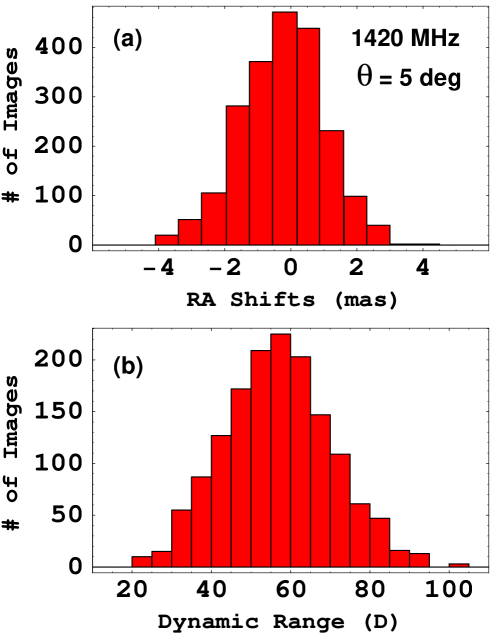
Figure 4: Distribution of right ascension shifts (a) and dynamic ranges (b) of 1500 snapshot phase-referenced images, simulated at 1420 MHz, for a 1 $\mu$Jy target source located at 5 deg from its calibrator. The calibrator source is located at an hour angle of 0 and the target source is located at the zenith of the array center.

5 Results

5.1 Observing frequency and signal decoherence

If the atmospheric turbulence is not taken into account and only the noise from the receivers is added to the visibilities, our simulations reproduce the dynamic ranges given by Eq. 6.53 of Thomson, Moran, & Swenson (TMS91 (1991)), as expected. Additionally, the noise from the receivers does not introduce considerable changes in the source position of the phase-referenced images (changes of the order of 10 $\mu$as or lower).

When the turbulent ionosphere and wet troposphere are added to the simulations, the dynamic range of the images is notably affected, especially at low ($<1\,GHz$) and high ($>10\,GHz$) frequencies. In Fig. 5, we show phase-referenced images of a 1 $\mu$Jy source, located at 5 deg. from its calibrator, observed at 0.5, 5, and 15 GHz. It can be readily seen that the addition of effects coming from the atmospheric turbulence maps into an important extra noise in the images at 0.5 and 15 GHz, but not at 5 GHz.

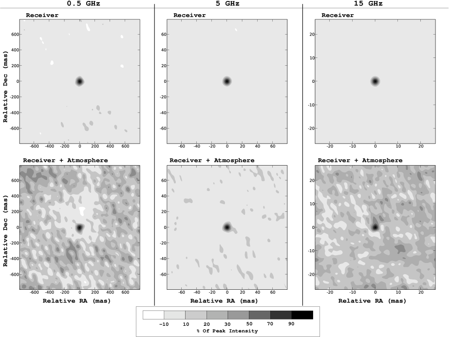
Figure 5: Simulated phase-reference images of a 1 $\mu$Jy source located at 5 deg from its calibrator. Noise from the receiving system (top) and, additionally, noise due to the turbulent atmosphere (bottom) have been added to the visibilities.

Following the algorithm described in Sect. 4, we obtained the astrometric uncertainties and dynamic ranges shown in Fig. 6. For very low frequencies (below $\sim$500 MHz) the ionosphere prevents a clear and precise detection of all sources, no matter their flux densities. For higher frequencies, the astrometric uncertainty decreases notably (mainly because of the dependence of ionospheric effects with $\nu^{-1}$) and gets limited only by diffraction and sensitivity between 1 and 10 GHz (this frequency window slightly depends on the source flux density, as it can be seen in the figure). For higher frequencies, the wet troposphere begins to affect the astrometric uncertainty, which rises up to around 10 mas for the highest frequencies. We find that the best astrometric accuracy, at least for reasonably well-detected sources, is achieved for frequencies around 4 GHz. This is where the ionospheric and (wet) tropospheric components are roughly equal.

Figure 6: Astrometric accuracy (a) and dynamic range (b) as a function of frequency, for the case with atmospheric turbulence and a separation of 5 degrees between calibrator and target. The calibrator source is located at an hour angle of 0 and the target source is located at the zenith of the array center. Different lines correspond to different target source flux densities (10 $\mu$Jy, continuous line; 1 $\mu$Jy, dashed line; 0.1 $\mu$Jy, dotted line).

The dynamic range of the phase-referenced images is highly limited by the atmosphere. When the atmosphere adds noise to the visibility phases, there is an extra rms added to the residual images, which depends on the visibility amplitudes, thus limiting the achievable dynamic range no matter the flux density of the source; that is, if the source flux density is higher, the noise of the image will also be higher. This limitation is, of course, more important for the brightest sources. In our case, the brightest source has a flux density of 10 $\mu$Jy. For this source, the maximum dynamic range achieved is only 110, which is $\sim 30$ times smaller than the dynamic range that would be obtained without the atmosphere. This situation can be also understood in another way: the rms of the final image is divided into two components, which are added in quadrature. One component, $\sigma_{th}$, comes from the receiver noise and is independent of the source flux density. The other component, $\sigma_{at}$, comes from the atmospheric refraction and is equal to a percentage of the source flux density ($\sigma_{at}=K_{r}\,S$, where $S$ is the source flux density and $K_{r}$ depends on the atmospheric refraction). Hence, the dynamic range, $D$, is

$$D=\frac{S}{\sqrt{\sigma_{th}^{2}+\sigma_{at}^{2}}}=\frac{S}{\sqrt{\sigma_{th}^{2}+K_{r}^{2}\,S^{2}}}$$ (3)

For large flux densities ($S>>\sigma_{th}$), the achievable dynamic range will saturate to a value dependent on the atmospheric conditions (i.e., $D\rightarrow 1/K_{r}$) and independent on the source flux density and the sensitivity of the stations. As seen in Fig. 6, despite of the large difference between the simulated flux densities (1 and 10 $\mu$Jy), the dynamic range saturates to a value of $\sim$100.

5.2 Angular separation and signal decoherence

The results shown in the previous subsection correspond to a separation of 5 degrees between source and calibrator. These results change when the angular separation changes. We computed astrometric uncertainties and dynamic ranges for a source with a flux densitity of 1 $\mu$Jy located at 2, 3, 4, 5, and 6 degrees from its calibrator. Noise from the atmosphere and the receivers was taken into account in these simulations. We used an observing frequency of 1420 MHz (the Hydrogen line) which is inside the frequency window where the atmospheric effects are minimised. Therefore, all the astrometric errors derived were small (of the order of a few mas), allowing us to use image sizes small enough to sample the beam with more pixels ($\sim$30 pixels) using a grid of 1024$\times$1024 pixels. This fine gridding of the beam allowed for a more accurate determination of the location of the image peak and, therefore, a better estimate of the astrometric error. The results obtained are shown in Fig. 7. In that figure, we also plot two analytical (phenomenological) models for the estimate of the increase of astrometric uncertainty and the loss of dynamic range (i.e., degree of signal decoherence) as a function of angular separation. On the one hand, the phenomenological model proposed for the estimate of loss of dynamic range is:

$$D=\frac{D_{0}}{\sqrt{1+k^{2}\,D_{0}^{2}\,\theta^{\beta}}},$$ (4)

where $D$ is the dynamic range, $\theta$ is the angular separation between target and calibrator, $D_{0}$ is the dynamic range without atmosphere (i.e., when the calibrator-to-target separation, $\theta$, tends to 0), and $k$ and $\beta$ are two parameters related to the atmospheric conditions, source flux density, and observing frequency. This equation is just Eq. 3, but setting $K_{r}=k\,\theta^{\beta/2}$.

As it can be seen, this model fits well to the simulations. We obtain $k=(2.5\pm 0.2)\times 10^{-5}$ deg^-β and $\beta=1.51\pm 0.06$.

Figure 7: Dots: simulated astrometric accuracy (a) and dynamic range (b) as a function of angular separation between calibrator and source, for observations at 1420 MHz and a target flux density of 1 $\mu$Jy. Lines: proposed phenomenological models.

On the other hand, the proposed phenomenological model for the increase of astrometric uncertainty is:

$$\sigma=\frac{\sigma_{0}}{D_{0}}\,(1+k^{\prime}\,\theta^{\beta^{\prime}}),$$ (5)

where $\sigma$ is the astrometric uncertainty, $\sigma_{0}$ is the diffraction limit (i.e., half the size of the beam), and $k^{\prime}$ and $\beta^{\prime}$ are two parameters also related to the atmospheric conditions, source flux density, and observing frequency. We fit $k^{\prime}=0.57\pm 0.04$ deg${}^{-\beta^{\prime}}$ and $\beta^{\prime}=1.02\pm 0.05$. From a different approach in the treatment of the noise from the atmosphere and limited to VLBA and EVN arrays, Pradel, Charlot, & Lestrade (Pradel (2006)) obtained a similar dependence of $\sigma$ with $\theta$.

We notice that if we change $D_{0}$ by $D$ in Eq. 5, the new fitted $k^{\prime}$ and $\beta^{\prime}$ are 1.03$\pm$0.09 and 0.07$\pm$0.06, respectively. This new value of $\beta^{\prime}$ is compatible with zero. In other words, the diffraction limit divided by the dynamic range of the image is an excellent estimator of the astrometric uncertainty, at least for the range of simulated calibrator-to-target separations at 1.4 GHz (which falls within the frequency window where the atmospheric effects are minimized).

For calibrator-to-target separations larger than $\sim$6 degrees, the situation changes. We simulated phase-referenced images for calibrator-to-target separations up to 12 degrees, and found that the model of dynamic range given by Eq. 4 is still valid, but the astrometric uncertainty increases faster, with $\beta^{\prime}=2.38\pm 0.08$ ($\beta^{\prime}=1.38$, if we change $D_{0}$ by $D$ in Eq. 4). This last $\beta^{\prime}$ fits well to the astrometric uncertainties for large source separations, but the fit is worse for separations smaller than 5-6 degrees.

5.3 Scalability of the results and use of turbulence models in the data calibration

In the previous subsections, we report on the effects of atmospheric turbulence in phase-referenced (and wide-field) interferometric images using fixed values for the Fried lengths of the Kolmogorov distributions of the ionosphere and wet troposphere. Since the Kolmogorov distribution is self-similar, the results reported can be scaled and adapted to other atmospheric conditions. Indeed, these simulations can also be used to estimate the limiting dynamic range and astrometric uncertainty if an a priori model of the tropospheric and/or ionospheric turbulence is used in the imaging. In these cases, the effective Fried length, $r_{ef}$, to compare to our simulations can be estimated as

$$r_{ef}=r_{0}\langle\frac{\phi_{mod}}{|\phi-\phi_{mod}|}\rangle$$ (6)

where $r_{0}$ is the Fried length of the real turbulence and the other factor is related to the fractional precision of the turbulence model: $\phi_{mod}$ is the phase computed from the turbulence model at a given point in the sky and $\phi$ is that corresponding to the real turbulence; the brackets $<...>$ represent averaging over the field of view. If the a priori model of the ionospheric electron distribution is accurate to a given precision level, the effective Fried length to use for the ionosphere will be that corresponding to the residual turbulence (i.e., the difference between the model and the real turbulence). For instance, in the case of a model of the ionospheric electron content with a 99% accuracy, the effective Fried length will be $r_{ef}=100\,r_{0}$; if the accuracy increases to 99.9%, $r_{ef}=1000\,r_{0}$. In Fig. 8, we show $D_{max}$, the maximum dynamic range (i.e., for a source with an infinite flux density, so $\sigma_{th}=0$ in Eq. 3) as a function of parameter $\eta$, which we define as

$$\eta=\frac{h\,\sin{\theta}}{r_{ef}}$$ (7)

In this equation, $h$ is the height of the phase screen and $\theta$ is the calibrator-to-target separation (or half the size of the wide-field image). Equation 7 can be used, together with Fig. 8, to compute the maximum achievable dynamic range for many different combinations of source separations, atmospheric conditions, and observing frequencies ($r_{ef}\propto\nu$ for the ionosphere and $r_{ef}\propto\nu^{-1}$ for the trosposphere). We notice, however, that Fig. 8 has been generated using only one Kolmogorov screen, so it is applicable to ionospheric dispersion (for low frequencies) or tropospheric dispersion (for high frequencies), but not to a situation where ionospheric and tropospheric effects are similar. In these cases, and as a first approximation, we could set

$$\eta=\frac{h_{ion}\,\sin{\theta}}{\sqrt{r_{ion}^{2}+\left(\frac{h_{ion}}{h_{trop}}r_{trop}\right)^{2}}}$$ (8)

where $r_{ion}$ and $r_{trop}$ are the (effective) Fried lengths of the ionosphere and troposphere, respectively, and $h_{ion}$ and $h_{trop}$ are the heights of each phase screen. Also shown in Fig. 8 is the fitting model

$$D_{max}=D_{1}\,\eta^{\beta_{1}}$$ (9)

where $D_{1}=48.38\pm 0.10$ and $\beta_{1}=-1.000\pm 0.002$. Figure 8 indicates how difficult is to obtain a high-contrast image with a wide-angle coverage at very low (or high) frequencies. For instance, an image of $10\times 10$ degrees with a dynamic range of $\sim$$10^{6}$ at a frequency of 500 MHz (which translates into $\eta\sim 5\times 10^{-5}$) would require, for the ionospheric screen used in the previous subsections, a model of the ionospheric turbulence distribution with an uncertainty lower than $3\times 10^{-5}$ (observing time of 1 minute). If the observing time increases to 10 hours, the minimum required uncertainty in the model of the ionosphere would increase to $7\times 10^{-4}$, but such a high precision should be kept during the whole set of observations. If the dynamic range decreases to $10^{5}$, the required minimum uncertainty for the ionosphere model would decrease to $7\times 10^{-3}$ (i.e., 0.7%) for an observing time of 10 hours.

Figure 8: Maximum dynamic range as a function of $\eta$ (see Eq. 7) and for a 1-scan snapshot of 60 s.

Figure 9: Peak flux density of the phase-referenced image, relative to the real peak flux density of the source, as a function of $\eta$ (see Eq. 7) and for a 1-scan snapshot of 60 s.

For a more comprehensive representation of our results, we show in Fig. 10 how the achievable dynamic range (computed from Eq. 9) depends on the uncertainty in the model of atmospheric turbulence used in the data calibration. We show this relationship for different observing frequencies and calibrator-to-target separations. For instance, a dynamic range $10^{4}$ in observations at 100 MHz for a calibrator-to-target separation of 1 deg. (i.e., the same for a wide-field image of $2\times 2$ deg.) would require a turbulence model with an accuracy of $\sim 99.9$% for an observing time of 60 s. This requirement would soften to an accuracy of $97-98$% for an observing time of 6000 s (provided the dynamic range increases as the square root of the observing time).

Figure 10: Maximum dynamic range as a function of the uncertainty in the model of the atmospheric turbulence for a 1-scan snapshot of 60 s.

For completeness, we also computed the loss of recovered flux density of the source due to the turbulent atmosphere. In Fig. 9 we show the ratio of peak flux densities between the phase-referenced images and those computed without the effects from atmospheric turbulence. For dynamic ranges of 40-50, the loss of flux density can be as large as 25%. The phenomenological model (also shown in the figure) used to fit the data is

$$\rho=\frac{1}{1+D_{2}\,\eta^{\beta_{2}}}$$ (10)

where $D_{2}=0.32\pm 0.02$ and $\beta_{2}=1.87\pm 0.01$.

Applicability of Eq. 9 and 10 is not restricted to the array used in the simulations here reported. The exponents $\beta_{1}$ and $\beta_{2}$ only depend on the structure of the atmospheric turbulence and are thus independent of the interferometer used in the observations. However, the parameters $D_{1}$ and $D_{2}$ also depend on the stations of the interferometer. Therefore, Eq. 9 and 10 can be adapted to any other interferometer by finding the right values of $D_{1}$ and $D_{2}$. As an example of this generalization of Eq. 9 and 10, Martí-Vidal et al. (MartiVidal2010 (2010)) have studied the achievable dynamic range in phase-referenced observations with the Very Long Baseline Array (VLBA) at 8.4 GHz and 15 GHz. This study has been performed from quasi-simultaneous observations of 13 sources located at separations ranging from 1.5 to 20.5 degrees. These authors have been able to model the dynamic ranges obtained in the phase-referenced images and the loss of recovered flux densities (phase-referenced images compared to images obtained from self-calibrated visibilities) using Eq. 9 and 10 with values for $D_{1}$ and $D_{2}$ different to those here reported, but using the same values here reported for the exponents $\beta_{1}$ and $\beta_{2}$.

6 Conclusions

We report on Monte Carlo estimates of the sensitivity and astrometric precision of an interferometric array, with a station distribution similar to that of the planned SKA, as a function of observing frequency, flux density, and source separation. These results can also be applied to other array distributions by taking into account the corresponding correction factors. Our estimates are based on simulations of snapshot phase-referenced observations, in which we take into account several effects from the turbulent atmosphere and the finite temperature of the receivers. We find that the astrometric uncertainty strongly depends on the observing frequency and smoothly increases as the source separation increases. For frequencies below $\sim$1 GHz, ionospheric effects dominate and the astrometry uncertainties (when the source is detectable) can be as large as $\sim$1 as. For frequencies between 1 and 10 GHz (these values slightly depend on the source flux density) atmospheric effects are minimum and we roughly reach the theoretical precision of the interferometer. Above these frequencies, the wet troposphere begins to dominate and the astrometric uncertainty increases to $\sim$10 mas for the highest simulated frequency (25 GHz). The dynamic range of the images is strongly limited by atmospheric turbulence at all frequencies and for all flux densities (it can decrease, in the worse cases, several orders of magnitude).

We propose analytical models for the loose of dynamic range and astrometric accuracy as a function of distance between calibrator and target source. These expressions could also be used to estimate the deformations and local dynamic ranges of wide-field images as a function of distance to the image phase center (i.e., the point in the sky where the data correlation is centered).

Appendix A Complementary simulations: different number of stations and array sensitivities

Our simulations are based on a given realization of the SKA. However, the main structure of the array distribution used in our simulations is not exclusive of the SKA. Other interferometric arrays, like ALMA or LOFAR, are being built with similar station distributions, consisting on a compact core and several extensions with the shape of spiral arms. Hence, our study can be extended to those arrays by taking into account the difference between the number of stations and the station sensitivities.

The amount of noise added to the data is proportional to the number of stations, since each station receives the signal through the turbulent atmosphere. However, for cases of clear source detections (D $>$ 20$-$30), the dynamic range does not depend (or the dependence is weak) on the thermal noise of the receivers (see Sect. 5.1). Therefore, to estimate the achievable dynamic range for an array with a different number of stations, the results shown in Fig. 6 should be divided by $N/N^{\prime}$, where $N$ is the number of stations used in our simulations ($N=200$) and $N^{\prime}$ is the number of stations of the other array. This is true for detections with a relatively large dynamic range ($D>20-30$). For weak sources, the noise from the receivers may also contribute to the rms of the residual images, so the factor to apply in these cases should be $(N\sigma^{\prime})/(N^{\prime}\sigma)$, where $\sigma$ is the thermal noise of the stations used in our simulations and $\sigma^{\prime}$ is that of the other array.

We repeated the simulations described in Sect. 5.1 using different arrays to compare the results with those obtained with the original array. On the one hand, we created a smaller array by subtracting 100 stations (those marked with empty squares in Fig. 1) from the original array. On the other hand, we created another array with all the 200 stations, but decreasing their sensitivity by a factor 2. We show the results obtained in Fig. 11. Special care must be taken in the interpretation of these figures, given that the computed ratios of dynamic ranges are only meaningful when the detections of the sources are clear (i.e. when no spurious noise peaks appear stronger than the source). This is true for D$>$20$-$30, which approximately corresponds to frequencies between 1 and 10 GHz (although it slightly depends on the source flux density, see Fig. 6).

With these considerations into account, we find that the ratio of dynamic ranges for the array with 100 stations falls between 0.7 and 0.5 compared to the array with 200 stations. The expected value is 0.5 (since $N^{\prime}=0.5N$ and $\sigma^{\prime}=\sigma$). Other factors, like the different coverages of Fourier space by both arrays, could be affecting the dynamic range of the images, thus increasing the ratio in some cases. For the array with lower station sensitivities (but the same number of stations), the ratio of dynamic ranges falls between 0.75 and 1 for the strongest sources (as expected, since $N^{\prime}=N$ and the noise from the receivers is much smaller than the noise from the atmosphere), while are close to 0.5 for the weakest source (also as expected, since the thermal noise from the receivers begins to dominate in this case).

Figure 11: Ratios of dynamic ranges obtained with our original array and those obtained with a subarray of 100 stations (a) and an array with half the sensitivity of the original array (b). Different lines correspond to different target source flux densities (10 $\mu$Jy, continuous line; 1 $\mu$Jy dashed line; 0.1 $\mu$Jy, dotted line).