Abstract

We discuss the holographic implications of torsional degrees of freedom in the context of AdS₄/CFT₃, emphasizing in particular the physical interpretation of the latter as carriers of the non-trivial gravitational magnetic field, i.e. the part of the magnetic field not determined by the frame field. As a concrete example we present a new exact 4-dimensional gravitational background with torsion and argue that it corresponds to the holographic dual of a 3d system undergoing parity symmetry breaking. Finally, we compare our new gravitational background with known wormhole solutions - with and without cosmological constant - and argue that they can all be unified under an intriguing ”Kalb-Ramond superconductivity” framework.

Torsional degrees of freedom in AdS₄/CFT₃

Department of Physics, University of Crete, Heraklion 71003, Greece

1 Introduction and summary of the results

AdS₄/CFT₃ is currently emerging as a novel paradigm of holography that has qualitatively different properties from the more familiar AdS₅/CFT₄ correspondence. Particularly intriguing is the recent accumulation of evidence that AdS₄/CFT₃ can be used to describe a plethora of phenomena in $2+1$ dimensional systems, such as quantum criticality [1, 2], Quantum Hall transitions [3, 4, 5, 6], superconductivity [7, 8, 9, 10, 11], supefluidity [12, 13] and spontaneous symmetry breaking [14, 15, 16]. This has given rise to a whole new research area that goes under the name of AdS/C(ondensed) M(atter) T(heory). Furthermore, AdS₄/CFT₃ is the appropriate setup to study the holographic consequences of generalized electric-magnetic duality of gravity and higher-spin gauge fields [17, 18, 19, 20, 21, 22].

In the absence of an explicit AdS₄/CFT₃ correspondence example various toy models have been used to study its general qualitative aspects. This work presents yet another model of AdS₄/CFT₃ which possesses a novel feature. Namely, it can describe the gravity dual of parity symmetry breaking in a 3d system. However, this is not our only aim. We also wish to shed light into torsion from a holographic point of view. The study of torsion is an interesting subject in itself that poses formal and phenomenological challenges. In the context of string theory, torsion is omnipresent through antisymmetric tensor fields, therefore AdS₄/CFT₃ provides the basic setup where it can be holographically investigated.

This review presents in a slightly expanded form the results of [34]. We consider a simple toy model where torsion is introduced via the topological Nieh-Yan class. In particular, we consider the modification of the Einstein-Hilbert action with a negative cosmological constant by the Nieh-Yan class, the latter having a spacetime-dependent coefficient. In the context of the 3+1-split formalism for gravity [17] we emphasize that the torsional degrees of freedom carry the non-trivial ‘gravitational magnetic field.’ In pure gravity the gravitational magnetic field is fully determined by the frame field and hence torsion vanishes. In our model, the spacetime dependence of the Nieh-Yan coefficient makes some of the components of the magnetic field dynamical and as a consequence torsional degrees of freedom enter the theory. Our toy model is simple enough such that only one of the torsional degrees of freedom becomes dynamical. This degree of freedom can be either carried by a pseudoscalar, in which case our model is equivalent to a massless pseudoscalar coupled to gravity, or by a two-form gauge potential. In the latter case our model becomes equivalent to a Kalb-Ramond field coupled to gravity.

Next, we find an exact solution of the equations of motion in Euclidean signature. Our metric ansatz is that of a bulk domain wall (DW). The solution, the torsion DW, has two distinct asymptotically AdS₄ regimes along the “radial” coordinate. The pseudoscalar has a kink-like profile and it is finite at both of the asymptotic regimes. Our torsion DW can be viewed as a generalization of the axionic wormhole solution of [35] in the case of non-zero cosmological constant. See also [36] for recent work on AdS wormholes.

Having in mind the holographic interpretation of our model we focus mainly on the case where the torsional degree of freedom is carried by a pseudoscalar field. Following standard holographic recipes we find that the torsion DW is the gravity dual of a 3d system that possesses two distinct parity breaking vacua. The two vacua are distinguished by the relative sign of the pseudoscalar order parameter. Our bulk picture suggests that the transition from one vacuum to the other can be done by a marginal deformation of the boundary theory. In the Appendix we suggest that the above qualitative properties can be realized in the boundary by the 3d Gross-Neveu model coupled to U(1) gauge fields.

Further, we point out that the bulk physics of our DW solution bears some intriguing resemblance to the standard Abrikosov vortex in superconducting systems. There is a natural mapping of the parameters of the torsion DW to those of the Abrikosov vortex. We show that the gravitational parameter that is interpreted as an order parameter satisfies a $\phi^{4}$-like equation and this motivates us to suggest that the cosmological constant is related to the “distance from the critical temperature” as $\Lambda\sim T_{c}-T$. However, there is an important difference in that the Abrikosov vortex is a one-dimensional defect while our DW is codimension one i.e. three-dimensional in AdS₄. We also discuss multi-DW configurations and DW condensation and show that $H$-flux supports bubbles of flat spacetime.

Quite intriguing is our result that DW condensation occurs at a critical value of the magnetic field. This motivates us to reconsider the known Euclidean solutions of an Einstein-axion system with [36] and without [35] cosmological constant. These are wormhole solutions whose salient properties include a quantized electric and (possibly) magnetic flux. Moreover, the $\Lambda\neq 0$ solutions possess a lower bound on their electric flux. Using our intuition that $\Lambda$ plays the role of ”temperature”, we place the known wormhole and DW solutions on a (”Temperature”,”Magnetic Field”) graph and observe that it resembles a standard superconductivity graph. We call such a system a ”Kalb-Ramond superconductor” and we will present more details on its properties in a forthcoming work [44].

2 Torsion as the non-trivial magnetic field of gravity

In this section we discuss the physical interpretation of torsion which is that it carries the non-trivial magnetic degrees of freedom of gravity, namely those that are not determined by the frame field (or, equivalently, by the metric in a 2nd order formulation). To motivate things we recall the first order formalism of electromagnetism in the presence of an $x$-dependent $\theta$-angle, in a non-trivial background here taken to be AdS₄. Then we present the 3+1-split formalism for gravity introduced in [17]. This formalism is a refined form of the standard ADM formalism, which however unveils the physical importance of the gravitational torsional d.o.f. As we will see, such a point of view is crucial in order to understand the holographic interpretation of torsion.

2.1 Electromagnetism with a $x$-dependent $\theta$-angle in AdS₄

The vierbeins and metric of AdS₄ are

$$e^{0}=dt\,,\,\,\,e^{\alpha}=e^{-t/L}dx^{\alpha}\,,\,\,\,ds^{2}=\sigma_{\perp}dt^{2}+e^{-2t/L}\eta_{\alpha\beta}dx^{\alpha}dx^{\beta}\,,$$ (1)

with $\alpha,\beta=1,2,3$. Throughout this work we are being flexible with the both the overall signature and also the nature (spacelilke or timelike) of the $t$-direction i.e.we set $\eta_{\alpha\beta}={\rm diag}(1,1,\sigma_{3})$, $\sigma_{\perp}\sigma_{3}=\sigma=\pm 1$. The gauge potential and field strength are one-forms

$$A=A_{0}dt+\tilde{A}\,,\,\,\,\,\,\,\,F=-dt\wedge E+\tilde{F}=\frac{1}{2}F_{ab}e^{a}\wedge e^{b}\,,$$ (2)

where $a,b=0,1,2,3$ and $E=-F_{0\alpha}e^{\alpha}$ is the electric field. The tilde will always denote quantities along the three directions $1,2,3$. With the above definitions we find

$$*_{4}F=dt\wedge*_{3}\tilde{F}-\sigma_{\perp}*_{3}E\,,\,\,\,dA=dt\wedge(\dot{\tilde{A}}-\tilde{d}A_{0})+\tilde{d}\tilde{A}\,.$$ (3)

Recall e.g. that $*_{3}e^{i}=\frac{1}{2}\epsilon^{i}_{\phantom{i}jk}e^{j}\wedge e^{k}$ and $*_{3}e^{i}\wedge e^{k}=\epsilon^{ij}_{\phantom{ij}k}e^{k}$. Note also that $*_{4}^{2}=\sigma_{\perp}$, $*_{3}^{2}=\sigma_{3}$ and $\epsilon_{0123}=1$. The first order action is

$$I=\int-dA\wedge*_{4}F+\frac{1}{2}F\wedge*_{4}F+\frac{\theta}{2}dA\wedge dA\,.$$ (4)

Notice that due to the $x$-dependance of $\theta$ the last term in (4) is not a total derivative and will give contributions to the e.o.m. After some work the action above takes the more familiar form

$$I = \sigma_{\perp}\int dt\wedge\left[\dot{\tilde{A}}\wedge\left(*_{3}E+\sigma_{\perp}\theta\tilde{d}\tilde{A}\right)+\frac{1}{2}\left(E\wedge*_{3}E-\sigma_{\perp}\tilde{F}\wedge*_{3}\tilde{F}\right)\right.$$ (5)

$$\hskip 56.9055pt+A_{0}\left(\tilde{d}*_{3}E+\sigma_{\perp}\tilde{d}\theta\wedge\tilde{d}\tilde{A}\right)\Bigl{]}\,.$$

This gives the Hamiltonian e.o.m.

$$E=-\dot{\tilde{A}}\,,\,\,\,\,\tilde{d}B=-\sigma_{\perp}\dot{\left(*_{3}E\right)}-\dot{\theta}\sigma_{3}*_{3}B-\tilde{d}\theta\wedge E\,,$$ (6)

where we have defined the magnetic field (also a one-form) as

$$\tilde{F}=\tilde{d}\tilde{A}\equiv\sigma_{3}(*_{3}B)\,.$$ (7)

We also have the Gauss law and Bianchi identity respectively

$$\tilde{d}*_{3}E+\sigma_{\perp}\tilde{d}\theta\wedge\tilde{d}\tilde{A}=0\,,\,\,\,\,\,\,\tilde{d}*_{3}B=0\,.$$ (8)

It is straightforward to show that the above give the Maxwell equations in the more familiar form

$$\vec{\nabla}\times\vec{E}=-\sigma_{3}\frac{\partial\vec{B}}{\partial t}\,,\,\,\,\,\,\,\vec{\nabla}\cdot\vec{E}=-\sigma_{\perp}\sigma_{3}\vec{\nabla}\theta\cdot\vec{B}\,,$$ (9)

$$\vec{\nabla}\times\vec{B}=-\sigma\frac{\partial\vec{E}}{\partial t}-\left[\dot{\theta}\vec{B}+\vec{\nabla}\theta\times\vec{E}\right]\,,\,\,\,\,\,\,\vec{\nabla}\cdot\vec{B}=0\,.$$ (10)

We summarize the effects of an $x$-dependent $\theta$-angle in electromagnetism:

• The modification of the canonical momentum as we see in (5)

  $$*_{3}E\mapsto*_{3}E+\sigma\theta*_{3}B\,.$$ (11)

• The presence of a source term for Gauss law.

In particular, there is no additional d.o.f. introduced by the $\theta$-angle. We will compare this situation with gravity in the following.

3 Details on the the 3+1-split formalism

In this section we present a concise version of the 3+1-split formalism of [17] for gravity in the presence of non-zero cosmological constant. We consider a globally hyperbolic Lorentzian manifold ${\cal M}$ and take the Einstein-Hilbert action with cosmological constant in the first-order Palatini formalism as

$$S_{{\rm EH}}=-\frac{1}{32\pi G}\int_{{\cal M}}\epsilon_{abcd}\left(R^{ab}+\frac{\Lambda}{2}e^{a}\wedge e^{b}\right)\wedge e^{c}\wedge e^{d}\,.$$ (12)

This is thus equivalent to the standard second-order gravitational action

$$S_{{\rm 2^{nd}}}=-\frac{1}{16\pi G}\int d^{4}x\sqrt{-g}\left(R+6\Lambda\right)\,,$$ (13)

and hence the cosmological constants is related to the parameter $\Lambda$ as $\Lambda_{\rm cosm.}=-3\Lambda$. The curvature and torsion 2-forms are defined in terms of the vielbein $e^{a}$ and spin-connection $\omega^{ab}$ as

$$R^{ab}=d\omega^{ab}+\omega^{a}{}_{c}\wedge\omega^{cb}\,,\qquad T^{a}=de^{a}+\omega^{a}{}_{b}\wedge e^{b}\,.$$ (14)

We define as before $\eta_{ab}={\rm diag}(\sigma_{\perp},+,+,\sigma_{3})$, where $\sigma_{\perp}\sigma_{3}=\sigma=\pm 1$, $\sigma_{\perp}^{2}=\sigma_{3}^{2}=1$ and set $\Lambda=\sigma_{\perp}/\ell^{2}$ such that $\Lambda<0$ ($\Lambda>0$) yields the de Sitter (Anti-de Sitter) vacuum. Next, we split the vielbein and the spin connection as

$$e^{0} = Ndt\,,\qquad e^{\alpha}=N^{\alpha}dt+\tilde{e}^{\alpha}\,,$$ (15)

$$\omega^{0\alpha} = q^{0\alpha}dt+\sigma_{\perp}K^{\alpha}\,,\qquad\omega^{\alpha\beta}=-\epsilon^{\alpha\beta\gamma}\left(Q_{\gamma}dt+B_{\gamma}\right)\,.$$ (16)

The novelty of the formalism is the introduction of the gravitational electric $K^{\alpha}$ and magnetic fields $B^{\alpha}$, which are both vector-valued one-forms on the slices. We then find for the torsion

$$T^{\alpha}=\tilde{T}^{\alpha}+dt\wedge\left\{\dot{\tilde{e}}^{\alpha}-\tilde{d}N^{\alpha}+NK^{\alpha}-\sigma{\epsilon^{\alpha}}_{\beta\gamma}Q^{\beta}e^{\gamma}-\sigma{\epsilon^{\alpha}}_{\beta\gamma}N^{\beta}B^{\gamma}\right\}\,,$$ (17)

$$T^{0}=\sigma_{\perp}K_{\alpha}\wedge\tilde{e}^{\alpha}+dt\wedge\left\{-\tilde{d}N-\sigma_{\perp}N_{\alpha}K^{\alpha}+{q^{0}}_{\beta}\tilde{e}^{\beta}\right\}\,,$$ (18)

and we write

$${R^{a}}_{b}=\tilde{R}^{a}_{\kern 5.0ptb}+dt\wedge r^{a}_{\kern 5.0ptb}\,,$$ (19)

$${\tilde{R}^{0}}_{\kern 5.0pt\alpha}=\sigma_{\perp}({\tilde{d}K}_{\alpha}+K_{\beta}\wedge\tilde{\omega}^{\beta}_{\kern 5.0pt\alpha})\equiv\sigma_{\perp}(\tilde{D}K)_{\alpha}\,,$$ (20)

$$\tilde{R}^{\alpha}_{\kern 5.0pt\beta}=^{(3)}\kern-5.0pt{R^{\alpha}}_{\beta}-\sigma_{\perp}K^{\alpha}\wedge K_{\beta}\,,$$ (21)

with

$${}^{(3)}R^{\alpha\beta}=\sigma\left[\epsilon^{\alpha\beta\gamma}dB_{\gamma}-\sigma_{\perp}B^{\alpha}\wedge B^{\beta}\right]\,,$$ (22)

and

$$2\epsilon_{\alpha\beta\gamma}r^{0\alpha}\wedge{\tilde{e}}^{\beta}\wedge{\tilde{e}}^{\gamma} = 2\sigma_{\perp}\epsilon_{\alpha\beta\gamma}\dot{K}^{\alpha}\wedge\tilde{e}^{\beta}\wedge\tilde{e}^{\gamma}+4Q_{\alpha}K_{\beta}\wedge\tilde{e}^{\beta}\wedge\tilde{e}^{\alpha}$$ (23)

$$+4q^{0\alpha}\left[\epsilon_{\alpha\beta\gamma}\tilde{T}^{\beta}\wedge\tilde{e}^{\gamma}\right]\,.$$

After some tedious but straightforward calculations we find

$$S_{EH} = -\frac{\sigma_{\perp}}{8\pi G}\int dt\wedge\Bigl{\{}\dot{\tilde{e}}^{\alpha}\wedge(4\sigma_{\perp}\epsilon_{\alpha\beta\gamma}K^{\gamma}\wedge\tilde{e}^{\beta})-4\sigma_{\perp}N^{\alpha}\epsilon_{\alpha\beta\gamma}(\tilde{D}K)^{\beta}\wedge{\tilde{e}}^{\gamma}$$ (24)

$$\hskip 28.45274pt+2N\epsilon_{\alpha\beta\gamma}\left({}^{(3)}R^{\alpha\beta}-\sigma_{\perp}K^{\alpha}\wedge K^{\beta}-\frac{\Lambda}{3}{\tilde{e}}^{\alpha}\wedge{\tilde{e}}^{\beta}\right)\wedge{\tilde{e}}^{\gamma}$$

$$\hskip 28.45274pt-4q^{0\alpha}\epsilon_{\alpha\beta\gamma}\tilde{T}^{\beta}\wedge\tilde{e}^{\gamma}+4Q_{\alpha}\tilde{e}^{\alpha}\wedge K_{\beta}\wedge\tilde{e}^{\beta}\Bigl{\}}-S_{GH}$$

where the last term is exactly the usual Gibbons-Hawking surface term

$$S_{GH}=-\frac{1}{16\pi G}\int_{\partial{\cal M}}\left(q^{0\alpha}dt+\sigma_{\perp}K^{\alpha}\right)\wedge\epsilon_{\alpha\beta\gamma}\tilde{e}^{\beta}\wedge\tilde{e}^{c}\,.$$ (25)

Adding then the Gibbons-Hawking term in (24) we obtain

$$\hat{S}_{EH} = -\frac{\sigma_{\perp}}{8\pi G}\int_{{\cal M}}dt\wedge\left\{-K_{\alpha}\wedge\dot{\Sigma}^{\alpha}+N\tilde{W}_{\alpha}\wedge\tilde{e}^{\alpha}+\sigma_{\perp}\hat{Q}\wedge K_{\beta}\wedge\tilde{e}^{\beta}\right.$$ (26)

$$\qquad\qquad\qquad\left.+\sigma_{\perp}q^{0\alpha}\tilde{D}\Sigma_{\alpha}-N^{\alpha}\epsilon_{\alpha\beta\gamma}\tilde{D}K^{\beta}\wedge\tilde{e}^{\gamma}\right\}\,,$$

where $\hat{Q}\equiv Q_{\alpha}\tilde{e}^{\alpha}$. We have introduced the 2-form

$$\tilde{W}_{\alpha}\equiv\rho_{\alpha}-\frac{1}{2}\epsilon_{\alpha\beta\gamma}K^{\beta}\wedge K^{\gamma}+\frac{1}{\ell^{2}}\Sigma_{\alpha}\,.$$ (27)

and have defined the oriented surface element as

$$\Sigma^{\alpha}=*_{3}\tilde{e}^{\alpha}=\frac{1}{2}\epsilon^{\alpha}{}_{\beta\gamma}\tilde{e}^{\beta}\wedge\tilde{e}^{\gamma}\,,$$ (28)

with $*_{3}$ the three-dimensional Hodge dual defined in terms of $\tilde{e}^{\alpha}$ only. The three-dimensional component of the curvature 2-form

$$\rho_{\alpha}=\tilde{d}B_{\alpha}+\frac{1}{2}\epsilon_{\alpha\beta\gamma}B^{\beta}\wedge B^{\gamma}\,,$$ (29)

is made out of $B^{\alpha}$ only. Recall (i.e. (19)) that $\tilde{D}$ is a covariant derivative with respect to the one-form field $B^{\alpha}$ as

$$\tilde{D}V^{\alpha}=\tilde{d}V^{\alpha}+\epsilon^{\alpha}_{\,\,\beta\gamma}B^{\beta}\wedge V^{\gamma}\,,$$ (30)

if $V^{\alpha}$ is a generic vector-valued one-form (with respect to either ${\rm SO}(3)$ or ${\rm SO}(2,1)$ depending on whether $\sigma_{\perp}=\mp 1$ respectively) defined on $\Sigma_{t}$. Comparing the action (26) to the electromagnetic action (4) motivates calling the vector-valued one-forms $K^{\alpha}$ and $B^{\alpha}$ the “electric” and “magnetic” fields respectively.

The action (26) is stationary on-shell when $\delta\tilde{e}^{\alpha}=0$ in the boundary, i. e. it provides a good Dirichlet variational principle with respect to the vielbein. The form of the action (26) appears to indicate that the proper conjugate dynamical variables are $\Sigma^{\alpha}$ (or, equivalently, $\tilde{e}^{\alpha}$) and $K^{\alpha}$. It has been shown in [19, 20] that the proper identification of the dynamical variables is slightly more involved than this. The remaining fields $\{N,N^{\alpha},q^{0\alpha},\hat{Q},B^{\alpha}\}$ enter the action as Lagrange multipliers of the following constraints:

$$-8\pi G\sigma_{\perp}\frac{\delta S}{\delta N} = \tilde{W}_{\alpha}\wedge\tilde{e}^{\alpha}=0\,,$$ (31)

$$-8\pi G\sigma_{\perp}\frac{\delta S}{\delta N^{\alpha}} = -\epsilon_{\alpha\beta\gamma}\tilde{D}K^{\beta}\wedge\tilde{e}^{\gamma}=0\,,$$ (32)

$$-8\pi G\sigma_{\perp}\frac{\delta S}{\delta q^{0\alpha}} = \sigma_{\perp}\tilde{D}\Sigma_{\alpha}=\sigma_{\perp}\epsilon_{\alpha\beta\gamma}\tilde{T}^{\beta}\wedge\tilde{e}^{\gamma}=0\,,$$ (33)

$$-8\pi G\sigma_{\perp}\frac{\delta S}{\delta\hat{Q}} = \sigma_{\perp}K_{\alpha}\wedge\tilde{e}^{\alpha}=0\,,$$ (34)

$$-8\pi G\sigma_{\perp}\frac{\delta S}{\delta B^{\alpha}} = N\tilde{T}^{\alpha}+\left(\tilde{d}N+\sigma_{\perp}K_{\beta}N^{\beta}-\hat{q}\right)\wedge\tilde{e}^{\alpha}=0\,,$$ (35)

where $\hat{q}\equiv q^{0}{}_{\alpha}\tilde{e}^{\alpha}$. The exterior multiplication of (35) by $\epsilon_{\alpha\beta\gamma}\tilde{e}^{\gamma}$ gives, by virtue of (33),

$$\tilde{d}N+\sigma_{\perp}K_{\beta}N^{\beta}-\hat{q}=0\,,$$ (36)

and hence we obtain the zero torsion condition

$$\tilde{T}^{\alpha}=\tilde{D}\tilde{e}^{\alpha}=0\,,$$ (37)

The last equation unveils the physical meaning of the gravitational magnetic field $B^{\alpha}$: it is a Lagrange multiplier which is algebraically related to the vielbein via the vanishing of torsion (37). This is exactly analogous to electromagnetism and gives an important hint regarding the relevance of torsion to holography and gravitational duality [34].

3.1 The analog of $\theta$-angle in gravity: the Nieh-Yan invariant

There is a number of topological terms built from the gravitational dynamical variables that one may consider in 4 dimension. These are all of potential interest to holography because being total derivatives they may induce interesting boundary effects. We may parameterize these terms as follows (writing all possible $SO(3,1)$-invariant 4-forms constructed from $e^{a},{R^{a}}_{b},T^{a}$):

$$I_{top}=n\int_{M}C_{NY}+2\gamma^{-1}\int_{M}C_{Im}+p\int_{M}P_{4}+q\int_{M}E_{4}\,,$$ (38)

where

$$C_{NY}=T^{a}\wedge T_{a}-R_{ab}\wedge e^{a}\wedge e^{b}=d(T^{a}\wedge e_{a})\,,$$ (39)

is the Nieh-Yan form. The parameter $\gamma$ is often referred to as the Immirzi parameter with

$$C_{Im}={R^{a}}_{b}\wedge e^{b}\wedge e_{a}\,.$$ (40)

The remaining objects are the Pontryagin form

$$P_{4}=-\frac{1}{8\pi^{2}}{R^{a}}_{b}\wedge{R^{b}}_{a}=-\frac{1}{8\pi^{2}}d({\omega^{a}}_{b}\wedge{R^{b}}_{a}-\frac{1}{3}{\omega^{a}}_{b}\wedge{\omega^{b}}_{c}\wedge{\omega^{c}}_{a})\,,$$ (41)

and the Euler form

$$E_{4}=-\frac{1}{32\pi^{2}}\epsilon_{abcd}R^{ab}\wedge R^{cd}\,.$$ (42)

We note that $P_{4}+\frac{\sigma_{\perp}a^{2}}{4\pi^{2}}C_{NY}$ and $C_{NY}-C_{Im}$ are actually $SO(3,2)$ invariants [30]. These terms become very interesting even in gravity if we allow the coefficients to become fields (for some interesting recent literature on the matter see [32, 33]).

3.2 Torsion and the magnetic field of gravity

In pure Eistein-Hilbert gravity the torsional d.o.f. are not dynamical and are carried by the magnetic field $B^{\alpha}$ . This is seen for example if we recall the definition of the non-trivial ‘spatial’ torsion as

$$\tilde{T}^{\alpha}=\tilde{d}\tilde{e}^{\alpha}-\sigma\epsilon^{\alpha\beta\gamma}B_{\beta}\wedge\tilde{e}_{\gamma}\,.$$ (43)

Moreover, it is seen from (18) that the radial component of torsion $T^{0}$ is determined by $\tilde{e}^{\alpha}$ and $K^{\alpha}$. Notice that (43) implies that the tensor $B_{\alpha\beta}$ is odd under ‘spatial’ parity, hence its trace $B^{\alpha}_{\,\,\alpha}$ is a pseudoscalar. Hence, although a priori the torsional degrees of freedom are not connected with the pair of conjugate variables $\tilde{e}^{\alpha}$ and $K^{\alpha}$, they are not dynamical as there is no kinetic term for $B^{\alpha}$. Rather, they enter (26) algebraically and as such they give via (35) and (36) the algebraic zero torsion condition (37) by virtue of which the magnetic field is related to the frame field. This is the gravitational analogue of the electromagnetic case where the magnetic field is related to the gauge potential via the Bianchi identity.

Consider now adding to the Einstein-Hilbert action the Nieh-Yan class $C_{NY}$ with a constant coefficient $\theta$. Over a compact manifold, the NY class is a topological invariant and takes integer values [30]. Having in mind holography, we are interested here in manifolds with boundary. In particular, the $3+1$ split has been set up so that the boundary is a constant-$t$ slice. The NY term reduces to a boundary contribution. The explicit calculation yields

$${\cal I}_{NY}\equiv-2\sigma_{\perp}\theta\int C_{NY}=2\sigma_{\perp}\theta\int dt\wedge\left[2\epsilon_{\alpha\beta\gamma}\dot{\tilde{e}}^{\alpha}\wedge\tilde{e}^{\beta}\wedge B^{\gamma}+\epsilon_{\alpha\beta\gamma}\dot{B}^{\alpha}\wedge\tilde{e}^{\beta}\wedge\tilde{e}^{\gamma}\right]$$ (44)

Adding (44) to (26) we obtain

$$\hat{S}_{EH}+{\cal I}_{NY} \propto \int dt\wedge\Bigl{(}\dot{\tilde{e}}^{\alpha}\wedge(-4\sigma_{\perp}\epsilon_{\alpha\beta\gamma}\tilde{e}^{\beta}\wedge\left[K^{\gamma}-\theta B^{\gamma}\right])$$ (45)

$$+2\sigma_{\perp}\theta\epsilon_{\alpha\beta\gamma}\dot{B}^{\alpha}\wedge\tilde{e}^{\beta}\wedge\tilde{e}^{\gamma}+\ {\rm constraint\ terms}\Bigl{)}\,.$$

Notice that the ${\cal I}_{NY}$ term has two effects. One is to modify the canonical momentum variable $K^{\alpha}\mapsto K^{\alpha}-\theta B^{\alpha}$. This is analogous to the effect of the $\theta$-angle in the canonical description of electromagnetism in section 2.1. The other is to provide a kinetic term for the singlet component of the magnetic field (one easily verifies that only ${B^{\alpha}}_{\alpha}$ contributes in the second term in the first line of (45)). This second effect has no analogue in electromagnetism. Taking the variation of (45) with respect to $B^{\alpha}$, one finds that the zero torsion condition still holds. This is expected of course since the ${\cal I}_{NY}$ term is purely a boundary term. As a consequence, the true dynamical variables remain $\tilde{e}^{\alpha}$ and $K^{\alpha}$. However, the holography is slightly modified. The variation of (45) gives on-shell

$$\delta\left(\hat{S}_{EH}+{\cal I}_{NY}\right)_{on\,\,shell}\propto\int_{\partial{\cal M}}\delta\tilde{e}^{\alpha}\wedge\left(-4\sigma_{\perp}\epsilon_{\alpha\beta\gamma}\tilde{e}^{\beta}\wedge\left[K^{\gamma}-\theta B^{\gamma}\right]\right)_{on\,\,shell}\,.$$ (46)

After the appropriate subtraction of divergences [19, 20], (46) yields a modified boundary energy momentum tensor. The modification is due to the term $4\sigma_{\perp}\theta\epsilon_{\alpha\beta\gamma}\tilde{e}^{\beta}\wedge B^{\gamma}$ which is parity odd and corresponds to the unique symmetric, conserved and traceless tensor of rank two and scaling dimension three that can be constructed from the three-dimensional metric [39]

$$T_{\alpha\beta}^{bdry}\mapsto T_{\alpha\beta}^{bdry}+\theta T_{\alpha\beta}^{top}\,,\,\,\,\,\,\,\,\,T_{\alpha\beta}^{top}\propto\epsilon_{\ell m(\alpha}\partial_{\ell}\partial^{2}g_{\beta)m}$$ (47)

where $g_{\alpha\beta}$ being the boundary metric. It is the exact analogue of the topological spin-1 current constructed from the 3d gauge potential [43, 39].

The form of the action (45) unveils an intriguing possibility. The above holographic interpretation was based on the zero torsion condition that connects $B^{\alpha}$ to the frame field. However, to get the zero torsion condition from (45) we needed to integrate by parts the last term in the first line. Hence, if $\theta$ were $t$-dependent, the torsion would no longer be zero and the trace $B^{\alpha}_{\,\,\alpha}$ would become a proper dynamical degree of freedom independent of $\tilde{e}^{\alpha}$. In such a case the holographic interpretation of (45) would change. The new bulk degree of freedom would couple to a new pseudoscalar boundary operator. As a consequence, we have the possibility to probe additional aspects of the boundary physics and describe new 2+1 dimensional phenomena. That we do in the next section.

4 The Nieh-Yan models

4.1 General aspects

In the previous section we sketched a mechanism by which torsional degrees of freedom become dynamical. In particular, we have argued that the addition of the Nieh-Yan class with a space-time-dependent coefficient in the Einstein-Hilbert action makes dynamical one pseudoscalar degree of freedom which is connected to the trace of the gravitational magnetic field. Adding boundary terms to the bulk action corresponds to a canonical transformation. Consequently, by adding boundary terms we can change the canonical interpretation and the variational principle. Consider first the action

$$I^{\prime}_{NY}=\hat{S}_{EH}[e,\omega]+I_{GH}[e,\omega]+2\int_{M}F(x)C_{NY}\,,$$ (48)

where $F$ is a pseudoscalar ‘axion’ field with no kinetic term. If $F\equiv-\sigma_{\perp}\theta$ were a constant, this theory would be equivalent to that studied in the last section. With $F=F(x)$, we have additional terms in the action involving gradients of $F$. If we perform the $3+1$ split on this action, we will find that $\tilde{e}^{\alpha}$ and $B^{\alpha}$ are canonical coordinates, and their conjugate momenta will depend on $F$.

The action as given may be supplemented by additional boundary terms. Such boundary terms are analogous to the Gibbons-Hawking term in gravity, but here involve the torsional degrees of freedom. In particular, we can replace $I^{\prime}_{NY}$ by

$$I_{NY}=\hat{S}_{EH}[e,\omega]+I_{GH}[e,\omega]-2\int_{M}dF\wedge T_{a}\wedge e^{a}\,.$$ (49)

This action is such that $\tilde{e}^{\alpha}$ and $F$ are canonical coordinates with appropriate boundary conditions, while $B^{\alpha}$ appears in the momentum conjugate to $F$. To investigate this theory, we note that the variation of the action takes the form

$$\delta I_{NY}=2\int_{M}\delta e^{d}\wedge\left[\epsilon_{abcd}e^{b}\wedge\left(R^{cd}-\frac{1}{3}\Lambda e^{c}\wedge e^{d}\right)+2dF\wedge T_{d}\right]$$

$$+2\int_{M}\delta\omega^{ab}\wedge\left[\epsilon_{abcd}T^{c}\wedge e^{d}+dF\wedge e_{b}\wedge e_{a}\right]+2\int_{M}\delta F\ C_{NY}$$

$$+2\int_{M}d[\delta e^{a}\wedge\left(\epsilon_{abcd}e^{b}\wedge\omega^{cd}-dF\wedge e_{a}\right)-T_{a}\wedge e^{a}\delta F]\,.$$ (50)

A non-trivial configuration of $F$ sources a particular component of the torsion. Indeed the classical equations of motion can be manipulated to yield in the bulk

$$T^{a}\wedge e_{a}=3*_{4}dF\,,$$ (51)

where $*_{4}$ denotes the Hodge-$*$ operation. However, as d’Auria and Regge [37] showed, this classical system is equivalent to a pseudoscalar coupled to torsionless gravity.

$$I_{PS}=\hat{S}_{EH}[e,\omega^{{}^{\kern-6.0pt\circ}}\kern 2.0pt]+I_{GH}[e,\omega^{{}^{\kern-6.0pt\circ}}\kern 2.0pt]-3\int_{M}dF\wedge*_{4}dF\,.$$ (52)

This comes about as follows. We write the connection as $\omega=\omega^{{}^{\kern-6.0pt\circ}}\kern 2.0pt+\Omega$, where $\omega^{{}^{\kern-6.0pt\circ}}\kern 2.0pt$ is torsionless, and insert the equation of motion (51). The latter becomes an equation for $\Omega$, and we obtain (52).

A massless pseudoscalar field coupled to torsionless gravity is holographically dual to composite pseudoscalar operators of dimensions $\Delta=3,0$ in the boundary. The usual holographic dictionary then says that only the $\Delta=3$ operator appears in the boundary theory since only this is above the unitarity bound of the 3d conformal group $SO(3,2)$. A scalar operator with dimension $\Delta=0$ would simply correspond to a constant in the boundary. Hence, the sensible holographic interpretation of the massless bulk pseudoscalar is that its leading behaviour determines the marginal coupling of a $\Delta=3$ operator; the expectation value of the operator itself is determined by the subleading behaviour of the bulk pseudoscalar.

Another equivalent formulation of this bulk theory is obtained by writing

$$*_{4}dF={\frac{1}{3}}H\,.$$ (53)

with $H$ a 3-form field. This is the parameterization that would be most familiar from string theory, as the system simply corresponds to an antisymmetric 2-form field. In this formulation, we write

$$I_{KR} = \hat{S}_{EH}[e,\omega^{{}^{\kern-6.0pt\circ}}\kern 2.0pt]+I_{GH}[e,\omega^{{}^{\kern-6.0pt\circ}}\kern 2.0pt]+\frac{1}{3}\int_{M}H\wedge*_{4}H+\sqrt{\frac{2}{3}}\int_{M}C\wedge d*_{4}H$$ (54)

$$= \hat{S}_{EH}[e,\omega^{{}^{\kern-6.0pt\circ}}\kern 2.0pt]+I_{GH}[e,\omega^{{}^{\kern-6.0pt\circ}}\kern 2.0pt]-\frac{1}{2}\int_{M}dC\wedge*_{4}dC+\int_{M}d(C\wedge*_{4}dC)\,.$$

In the first equation, $C$ appears as a Lagrange multiplier for the ‘Gauss constraint’ and in the second expression, we have solved for the $H$ equation of motion in the bulk, which is just $H=\sqrt{\frac{3}{2}}dC$.

4.2 The 3+1-split of the pseudoscalar Nieh-Yan model

To investigate the holographic aspects of our model it is most useful to use the ‘radial quantization’ in which we think of the radial coordinate as ‘time’ $t$. The Nieh-Yan deformation gives

$$-2\int dF\wedge T^{a}\wedge e_{a} = 2\int dt\wedge\Biggl{\{}-\dot{F}\tilde{T}_{\alpha}\wedge\tilde{e}^{\alpha}-\dot{\tilde{e}}_{\alpha}\wedge\tilde{d}F\wedge\tilde{e}^{\alpha}+N[2\tilde{d}F\wedge K_{\alpha}\wedge\tilde{e}^{\alpha}]$$ (55)

$$\hskip 28.45274pt+N^{\alpha}[2\tilde{d}F\wedge\tilde{T}_{\alpha}]+Q^{\alpha}[-\sigma\epsilon_{\alpha\beta\gamma}\tilde{d}F\wedge\tilde{e}^{\beta}\wedge\tilde{e}^{\gamma}]\Biggl{\}}\,.$$

We see that the $F$ field makes a contribution to the constraints, and has a conjugate momentum proportional to the scalar part of the torsion (the part transverse to the radial direction). The full bulk action becomes

$$I = \int dt\wedge\left(\dot{\tilde{e}}^{\alpha}\wedge(4\sigma_{\perp}\epsilon_{\alpha\beta\gamma}K^{\gamma}\wedge\tilde{e}^{\beta}-2\tilde{d}F\wedge\tilde{e}_{\alpha})-2\dot{F}(\tilde{e}^{\alpha}\wedge\tilde{T}_{\alpha})\right.$$ (56)

$$+N\left\{2\epsilon_{\alpha\beta\gamma}\left({}^{(3)}R^{\alpha\beta}-\sigma_{\perp}K^{\alpha}\wedge K^{\beta}-\frac{\Lambda}{3}{\tilde{e}}^{\alpha}\wedge{\tilde{e}}^{\beta}\right)\wedge{\tilde{e}}^{\gamma}+4\tilde{d}F\wedge K_{\alpha}\wedge\tilde{e}^{\alpha}\right\}$$

$$+4{N}^{\alpha}\left\{-\sigma_{\perp}\epsilon_{\alpha\beta\gamma}(\tilde{D}K)^{\beta}\wedge{\tilde{e}}^{\gamma}+\tilde{d}F\wedge\tilde{T}_{\alpha}\right\}$$

$$+4Q^{\alpha}\left\{(K_{\beta}\wedge\tilde{e}^{\beta})\wedge\tilde{e}_{\alpha}-\frac{1}{2}\sigma\epsilon_{\alpha\beta\gamma}\tilde{d}F\wedge\tilde{e}^{\beta}\wedge\tilde{e}^{\gamma}\right\}$$

$$+\left.4{q^{0}}_{\alpha}\left\{{\epsilon^{\alpha}}_{\beta\gamma}\tilde{T}^{\beta}\wedge\tilde{e}^{\gamma}\right\}\right)\,.$$

We notice that the $Q$-constraint term can be written in the form

$$4Q_{\alpha}\tilde{e}^{\alpha}\wedge\left(K_{\beta}\wedge\tilde{e}^{\beta}-\sigma*_{3}\tilde{d}F\right)\,.$$ (57)

Because of this constraint (which relates the antisymmetric part of the extrinsic curvature to the vorticity of $F$), the momentum conjugate to $\tilde{e}^{\alpha}$ is symmetric, i.e.

$$\Pi_{\alpha} = 4\sigma_{\perp}\epsilon_{\alpha\beta\gamma}K^{\gamma}\wedge\tilde{e}^{\beta}-2\tilde{d}F\wedge\tilde{e}_{\alpha}$$ (58)

$$= 4\sigma_{\perp}\left(\epsilon_{\alpha\beta\gamma}K^{\gamma}\wedge\tilde{e}^{\beta}-\frac{1}{2}\sigma_{3}*_{3}(K_{\beta}\wedge\tilde{e}^{\beta})\wedge\tilde{e}_{\alpha}\right)\,.$$

When written out in components, one finds that the antisymmetric part $K_{[\alpha\beta]}$ cancels

$$\Pi_{\alpha}=4\sigma_{\perp}(K_{(\beta\alpha)}-trK\ \eta_{\beta\alpha})\tilde{e}^{\beta}\,.$$ (59)

This result is consistent with the fact noted above, that the system may be equivalently described as a pseudoscalar field coupled to torsionless gravity. Moreover, if we take the deDonder gauge $d^{\dagger}\tilde{e}^{\alpha}=0$, the torsion constraint implies that $B$ is symmetric.

The ${q^{0}}_{\alpha}$ constraint yields ${\tilde{T}^{\beta}}_{\alpha\beta}=0$. Out of the nine components of $\tilde{T}$, which transform as ${\bf 5}+{\bf 3}+{\bf 1}$ under $SO(3)$ (or $SO(2,1)$), this sets the triplet to zero (the ${\bf 5}$ also vanishes on an equation of motion). The momentum conjugate to $F$ is given by

$$\Pi_{F}=-2\epsilon^{\alpha\beta\gamma}\tilde{T}_{\alpha\beta\gamma}\,.$$ (60)

This is the singlet part of the torsion, which has become dynamical in this description of the theory, in the sense that it is canonically conjugate to $F$.

5 The torsion domain wall

We will now simplify the analysis by taking a coordinate basis and looking for solutions of the form

$$\tilde{e}^{\alpha}=e^{A(t)}dx^{\alpha},\ \ \ \ N=1,\ \ \ \ N^{\alpha}=0\,,$$ (61)

and we will further suppose that $F=F(t)$. In this case $K^{\alpha}$ and $B^{\alpha}$ reduce to one degree of freedom each as a result of the constraints

$$K_{\alpha}=k\tilde{e}_{\alpha},\ \ \ \ B_{\alpha}=b\tilde{e}_{\alpha}\,,$$ (62)

and one finds $\Pi_{A}=-4\sigma_{\perp}k$ and $\Pi_{F}=2\sigma b$. The action then takes the following relatively simple Hamiltonian form

$$I_{NY}\propto\int dt\,d^{3}x\,\,e^{3A(t)}\left[\dot{A}\Pi_{A}+\dot{F}\Pi_{F}-\left(\frac{1}{2}\sigma_{3}\Pi_{F}^{2}+\frac{1}{8}\sigma_{\perp}\Pi_{A}^{2}+\frac{2}{3}\Lambda\right)\right]\,.$$ (63)

and the equations of motion give

$$\dot{\Pi}_{A}=3\dot{F}\Pi_{F},\ \ \ \ \ \ \dot{\Pi}_{F}+3\Pi_{F}\dot{A}=0,\ \ \ \ \ \ \Pi_{A}=4\sigma_{\perp}\dot{A},\ \ \ \ \ \Pi_{F}=\sigma_{3}\dot{F} \,,$$ (64)

$$\Pi_{A}^{2}+4\sigma\Pi_{F}^{2}+\frac{16}{3}\sigma_{\perp}\Lambda=0 \,.$$ (65)

These equations of motion could of course alternatively be obtained by considering the theory in the form (52). It is convenient to rescale $F(t)=\frac{1}{3}\Theta(t)$. Then the equations of motion can be put in the form

$$\dot{A}+3\dot{A}^{2}-3a^{2}=0,\ \ \ \ \ \ \dot{A}=\frac{1}{12}\sigma\dot{\Theta}^{2},\ \ \ \ \ \ \dot{\Theta}+3\dot{\Theta}\dot{A}=0\,.$$ (66)

where we have set $\Lambda=-3\sigma_{\perp}a^{2}$ with $a=1/L$. These are of the standard form of domain wall equations that have appeared numerous times in the AdS/CFT literature. However, there is a crucial difference. Notice that the first two of (66) imply

$$\dot{A}^{2}+\frac{1}{36}\sigma\dot{\Theta}^{2}-a^{2}=0\,.$$ (67)

For Euclidean signature ($\sigma=\sigma_{3}=1$) the second term in (67) has positive sign in contrast to most of the other holographic studies. This is due to the fact that in passing from Lorentzian to Euclidean signature the pseudoscalar kinetic term acquires the ‘wrong sign’ [40]. This property allows for a remarkable exact solution to the above system of non-linear equations in Euclidean signature, which we refer to as the torsion DW. To obtain it we define

$$h(t)=\dot{A}(t)\,,$$ (68)

at which point we have

$$\dot{h}=\frac{1}{12}\dot{\Theta}^{2},\ \ \ \dot{h}+3(h^{2}-a^{2})=0\,.$$ (69)

The general solution is of the form

$$h(t)=a\tanh 3a(t-t_{0})$$ (70)

and we then have

$$\Pi_{F}=\dot{F}=\pm 2\sqrt{a^{2}-h^{2}(t)}=\pm 2a\ \text{sech}\ 3a(t-t_{0})$$ (71)

which gives

$$\Theta(t)=\Theta_{0}\pm 4\arctan\left(e^{3a(t-t_{0})}\right)\,.$$ (72)

The $\pm$ sign corresponds to kink/antikink and we will without loss of generality choose the $+$ sign. We may also solve for

$$e^{A(t)}=\alpha(2\cosh 3a(t-t_{0}))^{1/3}$$ (73)

The parameter $\alpha$ is an arbitrary positive integration constant that sets the overall scale of the spatial part of the metric. $t_{0}$ may be interpreted as the position of the DW; when $t_{0}=0$ the torsion DW sits in the middle between the two asymptotically AdS₄ regimes. Below, we will discuss the interesting holographic interpretation of the torsion DW.

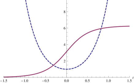
Figure 1: Plot of the torsion domain wall solution vs. $t$. The blue dashed line is $e^{A(t)}$ while the red solid line is $\Theta(t)$. To make the plot, we have chosen $\Theta_{0}=0$, $t_{0}=0$ and $\alpha=1$.

Note the curvature and torsion of this solution:

$${R^{\alpha}}_{\beta} = -\dot{F}\dot{A}\ {\epsilon^{\alpha}}_{\beta\gamma}dt\wedge e^{\gamma}-a^{2}e^{\alpha}\wedge e_{\beta}\,,$$ (74)

$${R^{\alpha}}_{0} = \left(\dot{h}+h^{2}\right)dt\wedge e^{\alpha}-\frac{1}{2}\dot{F}\dot{A}\ {\epsilon^{\alpha}}_{\beta\gamma}e^{\beta}\wedge e^{\gamma}\,,$$ (75)

$$T^{\alpha} = -\frac{1}{2}\dot{F}\ {\epsilon^{\alpha}}_{\beta\gamma}e^{\beta}\wedge e^{\gamma}\,,$$ (76)

$$T^{0} = 0\,.$$ (77)

These are non-singular for all $t\in(-\infty,\infty)$. The torsion DW solution has divergent action, but this divergence is cancelled by boundary counterterms, the same counterterms which render the action of $AdS_{4}$ finite. To see this, the energy of the torsion DW can be computed by evaluating the Euclidean action on the solution. Introducing a cutoff at $t=\pm L$, we find

$$I_{tv,on-shell} = 4a^{2}\int\epsilon_{\alpha\beta\gamma}dx^{\alpha}\wedge dx^{\beta}\wedge dx^{\gamma}\ \int dte^{3A(t)}$$ (78)

$$= (6\int\widehat{Vol}_{3})\cdot\left(\frac{4}{3}a\alpha^{3}e^{3aL}+\ldots\right)\,,$$ (79)

where the ellipsis contains terms that vanish when the cutoff is removed. As in pure $AdS_{4}$, an appropriate counterterm is of the form [41, 42]

$$I_{c.t.}=-\frac{4a}{3}\int_{\partial M}\epsilon_{\alpha\beta\gamma}\tilde{e}^{\alpha}\wedge\tilde{e}^{\beta}\wedge\tilde{e}^{\gamma}\,.$$ (80)

In the present case, we have such a counterterm on each asymptotic boundary, and thus we find

$$I_{c.t.}=-2\frac{2a}{3}\alpha^{3}e^{3aL}\cdot(6\int\widehat{Vol}_{3})\,,$$ (81)

which exactly cancels the divergent energy of the torsion DW.

Furthermore, we note that in the Kalb-Ramond representation, the solution has

$$H=\dot{\Theta}Vol_{3}=\pm 6a\alpha^{3}\widehat{Vol}_{3}\equiv\hat{H}\widehat{Vol}_{3}\,,$$ (82)

where $\widehat{Vol}_{3}=\frac{1}{6}\epsilon_{\alpha\beta\gamma}dx^{\alpha}\wedge dx^{\beta}\wedge dx^{\gamma}$. This corresponds to a ‘topological quantum number’ of the kink

$$\int*_{4}H=\pm\Delta\Theta=\pm 2\pi.$$ (83)

6 The torsion domain wall as the gravity dual of parity symmetry breaking

The holographic interpretation of the torsion DW is rather interesting. To study this, we set to zero without loss of generality the integration constant $\Theta_{0}=0$ and pick the plus sign in (71), (72). Next we need the asymptotic expansion of the vierbein which reads

$$\tilde{e}^{\alpha}=2^{-1/3}\alpha e^{\pm a(t-t_{0})}\left(1+\frac{1}{3}e^{\mp 6a(t-t_{0})}+\cdots\right)dx^{\alpha}\,\,\,{\rm for}\,\,\,t\rightarrow\pm\infty\,.$$ (84)

This shows that our solution is asymptotically anti-de Sitter for both $t\rightarrow\pm\infty$. The two asymptotic AdS spaces have the same cosmological constant. From this expansion we could read the expectation value of the renormalized boundary energy momentum tensor which would be given by the coefficient of the $e^{\pm 3at}$ term (see e.g. [19, 20]). Such a term is missing in (84), hence the expectation value of the boundary energy momentum tensor is zero.

It is not immediately apparent how to interpret these two asymptotic regimes. Are they truly distinct, or should they be identified in some way? We note that the pseudoscalar behaves in these asymptotic regimes as

$$\Theta(t) \rightarrow 4e^{-3a(t-t_{0})}-\frac{4}{3}e^{-9a(t-t_{0})}+\cdots\,\,\,{\rm for}\,\,\,t\rightarrow-\infty\,,$$ (85)

$$\Theta(t) \rightarrow 2\pi-4e^{3a(t-t_{0})}+\frac{4}{3}e^{9a(t-t_{0})}+\cdots\,\,\,{\rm for}\,\,\ t\rightarrow+\infty\,.$$ (86)

From the above we confirm that $\Theta(t)$ is dual to a dimension $\Delta=3$ boundary pseudoscalar that we denote ${\cal O}_{3}$. In each one of the asymptotically AdS regimes, the leading constant behavior of $\Theta(t)$ corresponds to the source (i.e., coupling constant) for ${\cal O}_{3}$ and the subleading term proportional to $e^{\mp 3a(t-t_{0})}$ to the expectation value $\langle{\cal O}_{3}\rangle$. The two asymptotic regimes are distinguished by the behavior of $\Theta$. In fact, the essential difference is parity.

We can now describe the holography of our torsion DW. In the $t\rightarrow-\infty$ boundary sits a three-dimensional CFT at a parity breaking vacuum state. The order parameter is the expectation value of the pseudoscalar which is $\langle{\cal O}_{3}\rangle=4$ in units of the AdS radius. The expectation value breaks of course the conformal invariance of the boundary theory. Then, the theory is deformed by the same pseudoscalar operator $g{\cal O}_{3}$ where $g$ is a marginal coupling. The torsion DW provides the holographic description of that deformation. Nevertheless, our solution should not be interpreted in terms of the usual holographic renormalization group flow. In our case, at $t\rightarrow+\infty$ the space becomes AdS with the same radius as at $t\to-\infty$. Hence, the two boundary theories have the same ‘central charges’.

We suggest that instead of interpreting the solution in terms of an RG flow, we should think of it as a domain wall transition between two inequivalent vacua of a single theory. This statement is supported by the behavior of $\Theta(t)$ in the two asymptotic regimes. For $t\rightarrow\infty$ the pseudoscalar asymptotes to the configuration (86). The interpretation is now that when the marginal coupling takes the fixed value $g_{*}=2\pi$ we are back to the same CFT (i.e. having the same central charge) however in a distinct parity breaking vacuum such that $\langle{\cal O}_{3}\rangle=-4$. In others words, the two asymptotic AdS regimes seem to describe two distinct parity breaking vacua of the same theory. The two vacua are distinguished by the expectation value of the parity breaking order parameter being $\langle{\cal O}_{3}\rangle=\pm 4$. Quite remarkably, we also seem to find that starting in one of the two vacua, we can reach the other by a marginal deformation with a fixed value of the deformation parameter.

Since the marginal operator is of dimension $\Delta=3$ and parity odd, we tentatively identify it with a Chern-Simons operator of a boundary gauge field. In this case the torsion DW induces the T-transformation in the boundary CFT [43, 39]. In Appendix A we will argue that the 3d Gross-Neveu model coupled to abelian gauge fields exhibits a large-$N$ vacuum structure that matches our holographic findings. Although our bulk model is extremely simple to provide details for its possible holographic dual, we regard this remarkable similarity as strong qualitative evidence that our torsion DW is the gravity dual of the ‘tunneling’ between different parity breaking vacua in three dimensions. However, in a three-dimensional quantum field theory, we do not expect that tunneling can occur because of large volume effects, and distinct vacua remain orthogonal. Thus, referring to the torsion DW as a tunneling event should be taken figuratively. We leave to future work a more careful study of the boundary interpretation of the torsion DW solution. An interpretation will depend on the precise topology of the boundary.[44] Moreover, embedding our model into M-theory could provide additional clues regarding its holography.

7 Physics in the bulk: the superconductor analogy

The bulk interpretation of the exact solution is also interesting. Because the pseudoscalar field undergoes $\Theta(t)\to\Theta(t)+2\pi$ under $t$ goes from $-\infty$ to $+\infty$, the exact solution corresponds to a topological kink. It satisfies

$$\int dt\dot{\Theta}=2\pi$$

In Figure 2, we plot the solution.

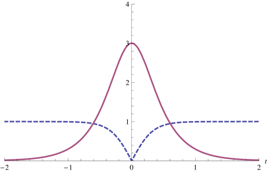
Figure 2: The blue dashed line is $|h(t)|$, resembling the order parameter of a superconductor, while the solid red line is $\Pi_{F}$, analogous to the magnetic induction of an Abrikosov DW.

7.1 Torsion domain wall vs Abrikosov vortex

The gravity DW solution (69–72) bears some resemblance to the Abrikosov vortex of superconducting systems. To avoid confusion we emphasise here that this is not a holographic interpretation i.e. the Abrikosov vortex (or more precisely, domain wall) is in the bulk. In this section, we will explore this and point out some possibly interesting features. The first thing to notice is that the plot in Fig. 2 is identical to the profile of an Abrikosov vortex (see for example Figure 5.1 in Ref. [45].) The codimension differs and this is expected; the torsion DW supports a 3-form field strength in contrast to a 2-form field strength supported by the Abrikosov vortex. Nevertheless, there is a correspondence between our radial $t$-direction and the radial direction in the Abrikosov vortex, and $|h|$ and $\Pi_{F}$ correspond to the condensate and magnetic induction of the superconductor, respectively. Table 1 summarizes the correspondence.

Abrikosov vortex	Torsion DW
order parameter $\Phi$	order parameter $|h|=|{\dot{A}}|$
$T-T_{c}$	$\Lambda$
magnetic induction B	$\Pi_{F}$
magnetic field H	$\hat{H}$
$\mathbb{Z}$-quantized magnetic flux	$\mathbb{Z}_{2}$-quantized electric flux

Table 1: Abrikosov vortex v.s. Torsion DW

In this correspondence, since the order parameter is $h=\dot{A}$, the superconducting phase (constant order parameter) corresponds to $AdS_{4}$, while the normal phase corresponds to flat space ($h=0$). Far away from the core of the torsion DW, the geometry is asymptotically $AdS$, but at the core the spatial slice (at $t\to t_{0}$) becomes flat. To see this, note that if we think of the system as a pseudoscalar coupled to torsionless gravity, the torsion DW has ${\omega^{{}^{\kern-6.0pt\circ}}\kern 2.0pt^{\alpha}}_{\beta}=0$ and ${\omega^{{}^{\kern-6.0pt\circ}}\kern 2.0pt^{\alpha}}_{0}=\dot{A}\tilde{e}^{\alpha}$, and so

$${R^{{}^{\kern-6.0pt\circ}}\kern 2.0pt^{\alpha}}_{\beta} = -h^{2}\tilde{e}^{\alpha}\wedge\tilde{e}_{\beta}\,,$$ (87)

$${R^{{}^{\kern-6.0pt\circ}}\kern 2.0pt^{\alpha}}_{0} = (\dot{h}+h^{2})dt\wedge\tilde{e}^{\alpha}\,,$$ (88)

$$T^{{}^{\kern-6.0pt\circ}}\kern 2.0pt^{\alpha} = 0\,.$$ (89)

Thus, at the core, we find that the Riemann tensor has components

$${R^{\alpha}}_{0\alpha 0} \to-3a^{2}\alpha\,,$$ (90)

$${R^{\alpha}}_{\beta\alpha\beta} \to 0\,.$$ (91)

This behavior is in line with an Abrikosov vortex in which there is normal phase at the core and superconducting phase away from the core.

The analogue of the magnetic field is what we have called $\hat{H}$, proportional to the constant $\alpha^{3}$. In the DW, the magnetic induction, analogous to $\Pi_{F}$, has a penetration length $\lambda\sim 1/3a$, and the coherence length of the order parameter is $\xi\sim 1/6a$. The penetration and coherence lengths are obtained by looking at the exponential fall-off of these quantities in the core of the DW, away from their values in the superconducting phase.

The torsion DW also has a quantized flux $\int*_{4}H=\Delta\Theta=2\pi$. This flux is independent of any parameters of the solution and of any rescaling of fields in the theory. Thus, this is an analogue of the quantized magnetic flux in superconductivity.

Finally, note the following interesting feature. If we take a derivative of the second equation in (69), we arrive at

$$\ddot{h}-6\Lambda h-18h^{3}=0\,.$$ (92)

This looks like a Landau-Ginzburg equation of motion of an effective $\phi^{4}$ theory. This leads us to interpret

$$\Lambda=-3\sigma_{\perp}a^{2}=-3\sigma_{\perp}\frac{1}{L^{2}}\sim T_{c}-T$$ (93)

Of course, there is no real temperature in the case of the torsion DW, but we note that this implies that the penetration and coherence lengths diverge as

$$(T-T_{c})^{1/2}$$ (94)

i.e. with a mean field theory critical exponent $1/2$, as in superconductivity.

7.2 Domain wall condensation: a prelude to Kalb-Ramond superconductivity?

In the last section, we noted that there is a strong analogue between the torsion DW solution and superconductivity. It is intriguing to carry the analogy further and consider multi-DW configurations. We have noted that at the core of the torsion DW, the spatial sections are flat. Thus, one might imagine that if it was favourable for torsion DWs to condense, as DWs do in Type I superconductors, then finite regions of normal phase (corresponding to $\Lambda=0$) would be obtained. We will argue below that this can in fact occur, although the system appears not to be unstable.

To understand the physics involved, the first step is to consider a configuration of two DWs. In the superconductivity literature, this is a standard computation. One takes two DWs separated by a distance $\ell$ and computes the Euclidean action. More precisely, we will treat this here as follows. Put the system in a box by restricting the $t\in[-L,L]$. In such a case, a DW located at $t_{0}$ has on-shell action

$$e^{A(t-t_{0})}=\alpha(2\cosh 3a(t-t_{0}))^{\frac{1}{3}}\Rightarrow I^{L}_{on-shell}=\left(6\hat{Vol}_{3}\right)\frac{4}{3}a\alpha^{3}e^{3a(L-t_{0})}\,.$$ (95)

We then consider a piecewise solution of two DWs located at $t=\pm\frac{L}{2}$ This is not a solution of the e.o.m. because solutions of non-linear equations cannot be simply superimposed i.e. it fails at the midpoint between the DWs. However, if we simply evaluate the Euclidean action, we find

$$I^{\pm(L/2)}_{on-shell}=\left(\frac{4}{3}a^{2}\hat{Vol}_{3}\right)4a\alpha^{3}\sinh\frac{3aL}{2}\,.$$ (96)

Note that this is positive, so one might naively conclude that the DWs repel each other. However, recall that the DW profile exists not in flat space-time, but in the metric given by (73), which rises asymptotically. As a result, as we move the DWs further apart, there is a corresponding rise in the metric between the DWs. So, we should directly evaluate the force at a point $t=\ell$ as

$$F=-\frac{dI^{\pm(L/2)}}{d\ell}\propto\cosh(3a\ell/2)<0\,.$$ (97)

Thus we conclude that the DWs in fact attract each other. In the superconducting analogue we would conclude that we have a Type I superconductor where the vortices clump together forming (potentially) finite regions of normal phase. In such a superconductor, the number of vortices is determined by the total magnetic flux.

We now describe the analogous situation in our gravitational system. We have noted that the constant $\hat{H}$ plays the role of the external magnetic induction, while $H$ is the magnetic field, varying within the DW, with $\Delta\Theta=\int*_{4}H$. Following the superconducting analogue, if we put the system in a box of size $2L$ (that is we impose a cutoff on each AdS asymptotic) the flux conservation equation is of the form

$$\Delta\Theta=2L\hat{H}$$ (98)

The DWs carry the flux in the superconductor, and so it is natural to ask what is the lowest energy configuration satisfying (98)? To analyze this, consider an array of $n$ DWs in a region of size $L_{0}$. We take the DWs to be equally spaced, as one can show that deviating from such a configuration causes a rise in energy. For such a configuration, the flux quantization condition (98) gives a relation between $n$,$L_{0}$ and $\hat{H}$. Such a representative curve is shown in Fig. 3

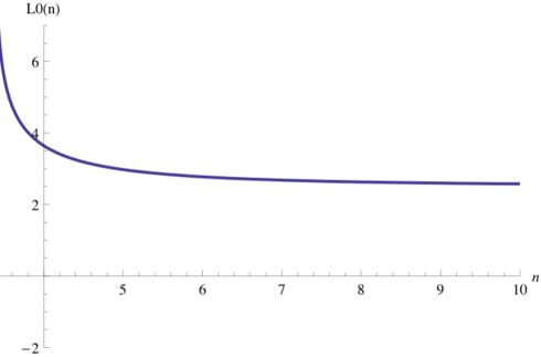
Figure 3: Size of normal state droplet vs. $n$ for multi-domain walls.

If we solve this equation for $L_{0}$ as a function of $n$ and $\hat{H}$, we can then compute the energy as a function of $n$. One obtains a curve as in Fig. 4.

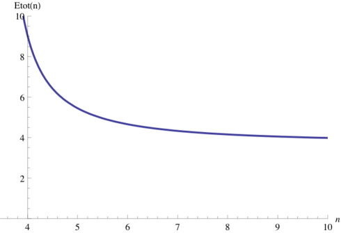
Figure 4: Energy vs. $n$ for multi-domain walls.

One notes that the energy is minimized for large $n$, and in that case, the size $L_{0}$ asymptotes to a fixed value, which is found to be

$$L_{0}=\frac{\hat{H}}{6a}\cdot 2L=\alpha^{3}\cdot 2L$$ (99)

We conclude that the preferred configuration, given a fixed external flux, is a continuum of DWs arrayed over a finite size region. Within this droplet, the system is in the normal phase. We have noted that the DW core is spatially flat, and so we surmise that within the droplet, the space-time is flat. The asymptotic value of energy in Figure 4 is precisely minus that contributed by the cosmological constant. Again, the size of the droplet is set by the value of the external $H$-flux, and the boundary conditions are AdS. Note that for a fixed cutoff, there is a critical field (given by $\hat{H}=6a$) for which the entire spacetime is flat.

The result above motivate us to take a further step and suggest rather appealing physical picture that we may call Kalb-Ramond superconductivity. Here we present a qualitative description of Kalb-Ramond superconductivity. A detailed description will appear shortly in [44]. As discussed above, minus the cosmological constant may be interpreted as $T-T_{c}$. This, together with the interpretation of $H$ as a magnetic induction and $\hat{H}=6a$ as a critical magnetic field above which the spacetime is flat due to DW condensation, motivates to draw a $-\Lambda,*H$ graph analogously with the $T-T_{c},$magnetic field graph in superconductivity. To do so, we need to consider all known solutions of an Einstein-axion system in $d=4$ with and without cosmological constant. For $\Lambda=0$ we recall the axionic DW solutions of [35]. For $\Lambda<0$ DW wormhole-like solutions were found in [36].

These solutions have the following properties (to be discussed in more detail in [44]):

The $\Lambda=0$ wormhole solution [35] is asymptotically flat. Its magnetic flux is proportional to an arbitrary constant $g$ which was speculated to be quantized via a string theory embedding of the Einstein-axion system. in [35]. Its electric flux is $\mathbb{Z}_{2}$-quantized to $\pm 3\pi$, but the electric field varies along the wormhole.

The $\Lambda<0$ wormhole solution [36] is asymptotically AdS. Its magnetic flux is also proportional to the arbitrary constant $g$, and hence possibly quantized in a string theory embedding. Quite intriguingly, the electric flux on the wormhole solution interpolates between the value $\pm 3\pi$ for $g\rightarrow 0$ and $\pm 2\pi$ as $g\rightarrow\infty$. Moreover, there is a lower bound for magnetic field of the wormhole solution. Remarkably, this lower bound is the value $6a$ and coincides with the maximal magnetic field of the torsion DW.

In Fig. 5 we sketch the possible phase diagram of the Kalb-ramond superconductor. Our torsion DW solution seems to play the role of the superconducting phase, while the wormhole solutions of [35] and [36] appear to correspond to the normal phase.

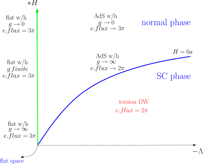
Figure 5: A sketch of the phase diagram for a Kalb-Ramond superconductor.

8 Conclusions

In this work we have presented in detail a simple toy model, the Nieh-Yan model, where torsion enters through the spacetime dependence of the coupling constant of the Nieh-Yan topological invariant. Although we have discussed the model directly in terms of torsion, it can classically be put into equivalent forms as either a massless pseudoscalar or a Kalb-Ramond field coupled to gravity. The model has an interesting and non-trivial holographic interpretation. In particular, we have shown that it possesses an exact bulk solution in Euclidean signature, termed the torsion DW, having two asymptotically AdS₄ regimes, while the pseudoscalar acquires a kink profile. We have argued then that the holographic interpretation of this torsion DW is a three-dimensional CFT with two distinct parity breaking vacua. Moreover, our bulk solution may imply that the deformation by a classically marginal pseudoscalar with a fixed coupling constant induces a transition between the two parity breaking vacua separated by a domain wall, which would be at infinity in the boundary components.[44] Remarkably, this qualitative behaviour is seen already in the three-dimensional Gross-Neveu model coupled to $U(1)$ gauge fields. The economy of our bulk model does not allow a detailed identification of the bulk and boundary theories, nevertheless we believe that our results provide a strong base where an exact bulk/boundary dictionary for AdS₄/CFT₃ can be based. A further rather intriguing property of the torsion DW is that it can be mapped into the standard Abrikosov vortex of superconductivity. Such a map identifies flat spacetime with a superconductor’s normal phase, while AdS is identified with a superconducting phase. The cosmological constant would then measure the deviation from the ‘critical temperature’. A phenomenon of DW condensation is found, similar to the analogous case in type I superconductors. Finally, we have briefly discussed a picture of ”Kalb-Ramond superconductivity” that emerges if we view in a unified way all known 4-dimensional Euclidean solutions of the Einstein-axion system. This picture will be furhter analysed in [44].

Our results indicate that the torsional degrees of freedom of four dimensional gravity can provide holographic descriptions for a number of interesting properties of 3d critical systems. It would be interesting to extend our analysis to more elaborate models where more torsional degrees of freedom become dynamical. It is also of interest to discuss whether our simple model can be embedded into M-theory.

Acknowledgments

I thank the organizers and in particular Lefteris Papantonopoulos for the organization of a top quality workshop and the invitation to present this talk. This work is partially supported by the FP7-REGPOT-2008-1 ”CreteHEPCosmo” No 228644 and also by the University of Crete ELKE grant with KA 2745. I wish to thank R. G. Leigh and N. N. Hoang for the very fruitful and pleasant collaboration that has led to the results presented in this report.

Appendix A Parity breaking in three dimensions

Consider the 3d Gross-Neveu model coupled to abelian gauge fields. The Euclidean action is

$$I=-\int d^{3}x\left[\bar{\psi}^{a}\left(/\!\!\!\partial-{\rm i}e/\!\!\!\!A\right)\psi^{a}+\frac{G}{2N}\left(\bar{\psi}^{a}\psi^{a}\right)^{2}+\frac{1}{4M}F_{\mu\nu}F_{\mu\nu}\right]\,.$$ (A.1)

$M$ is an UV mass scale. Introducing the usual Lagrange multiplier field $\sigma$, whose equation of motion is $\sigma=\frac{-2G}{N}\bar{\psi}^{a}\psi^{a}$ we can make the action quadratic in the fermions

$$I=-\int d^{3}x\left[\bar{\psi}^{a}\left(/\!\!\!\partial+\sigma-{\rm i}e/\!\!\!\!A\right)\psi^{a}-\frac{N}{2G}\sigma^{2}-\frac{1}{4M}F^{\mu\nu}F_{\mu\nu}\right]\,.$$ (A.2)

The model possesses two parity breaking vacua distinguished by the value of the pseudoscalar order parameter $\langle\sigma\rangle$. This is seen as follows: switching off the gauge fields momentarily one integrates over the fermions to produce a large-$N$ effective action as

$${\cal Z}=\int({\cal D}\sigma)e^{N\left[{\rm Tr}\log\left(/\!\!\!\partial+\sigma\right)-\frac{1}{2G}\int d^{3}x\sigma^{2}\right]}\,.$$ (A.3)

The path integral has a non-zero large-$N$ extremum $\sigma_{*}$ found by setting $\sigma=\sigma_{*}+\frac{1}{\sqrt{N}}\lambda$

$${\cal Z}=\int({\cal D}\lambda)e^{N\left[{\rm Tr}\log\left(/\!\!\!\partial+\sigma_{*}\right)-\frac{1}{2G}\int d^{3}x\sigma_{*}+\frac{1}{\sqrt{N}}\left\{{\rm Tr}\frac{\lambda}{/\!\!\!\partial+\sigma_{*}}-\frac{\sigma_{*}}{G}\int d^{3}x\lambda\right\}+O(1/N)\right]}$$ (A.4)

The term in the curly brackets is the gap equation. To study it one considers a uniform momentum cutoff $\Lambda$ to obtain

$$\frac{1}{G}=\int^{\Lambda}\frac{d^{3}p}{(2\pi)^{3}}\frac{2}{p^{2}+\sigma_{*}^{2}}=({\rm Tr}1)\left[\frac{\Lambda}{\pi^{2}}-\frac{|\sigma_{*}|}{\pi^{2}}\arctan\frac{\Lambda}{|\sigma_{*}|}\right]\,.$$ (A.5)

Defining the critical coupling as

$$\frac{1}{G_{*}}=\frac{\Lambda}{\pi^{2}}\,,$$ (A.6)

(A.5) possesses a non-zero solution for $\sigma_{*}$ when $G>G_{*}$ given by

$$|\sigma_{*}|=\frac{2\pi}{G}\left(\frac{G}{G_{*}}-1\right)\equiv m\,.$$ (A.7)

The two distinct parity breaking vacua then have

$$\sigma_{*}=-\frac{2G}{N}\langle\bar{\psi}^{a}\psi^{a}\rangle=\pm m\,.$$ (A.8)

Going back to (A.2) one can tune $G>G_{*}$ and start in any of the two parity breaking vacua. Suppose we start from $\sigma_{*}=+m$. To leading order in $N$ we have

$${\cal Z} = \int({\cal D}A_{\mu})({\cal D}\bar{\psi}^{a})({\cal D}\psi^{a})\exp[{\cal S}]$$ (A.9)

$${\cal S} = \int d^{3}x\left[\bar{\psi}^{a}\left(/\!\!\!\partial+m-{\rm i}e/\!\!\!\!A\right)\psi^{a}-\frac{N}{2G}m^{2}+O(1/\sqrt{N})-\frac{1}{4M}F^{\mu\nu}F_{\mu\nu}\right]$$

As is well known [46, 47] for $N$ fermions the path integral (A.9) yields an effective action for the gauge fields which for low momenta is dominated by the Chern-Simons term i.e.

$${\cal Z}\approx\int e^{S_{CS}}\,,$$ (A.10)

with

$$S_{CS}={\rm i}\frac{ke^{2}}{4\pi}\int d^{3}x\epsilon^{\mu\nu\rho}A_{\mu}\partial_{\nu}A_{\rho}\,,\,\,\,\,\,\,\,\,k=\frac{N}{2}\,.$$ (A.11)

Had we started from the $\sigma_{*}=-m$ vacuum, we would have found again (A.10)-(A.11), however with $k=-\frac{N}{2}$, i.e. the vacuum with $\sigma_{*}=-m$ yields an effective Chern-Simons action with $k=-\frac{N}{2}$.

Consider now deforming the action (A.9) by the Chern-Simons term with a fixed coefficient as

$${\cal Z}_{deform} = \int({\cal D}A_{\mu})({\cal D}\bar{\psi}^{i})({\cal D}\psi^{i})\exp[{\cal S}_{def}]$$ (A.12)

$${\cal S}_{def} = {\cal S}-{\rm i}q\int d^{3}x\epsilon^{\mu\nu\rho}A_{\mu}\partial_{\nu}A_{\rho}$$

If $q$ is fixed to

$$q=\frac{Ne^{2}}{4\pi}\,,$$ (A.13)

the effective action for the gauge fields resulting from the fermionic path integrals in (A.12) is going to be equal to the one obtained had we started at the $\sigma_{*}=-m$ vacuum. In other words, deforming the $\sigma_{*}=+m$ vacuum with a Chern-Simons term with a fixed coefficient is equivalent to being in the $\sigma_{*}=-m$ vacuum. This is exactly analogous to the holographic interpretation of our torsion DW.

References

- [1] C. P. Herzog, P. Kovtun, S. Sachdev, and D. T. Son, “Quantum critical transport, duality, and M-theory,” Phys. Rev. D75 (2007) 085020, arXiv:hep-th/0701036.
- [2] S. A. Hartnoll, P. K. Kovtun, M. Muller, and S. Sachdev, “Theory of the Nernst effect near quantum phase transitions in condensed matter, and in dyonic black holes,” Phys. Rev. B76 (2007) 144502, arXiv:0706.3215.
- [3] S. A. Hartnoll and P. Kovtun, “Hall conductivity from dyonic black holes,” Phys. Rev. D76 (2007) 066001, arXiv:0704.1160.
- [4] S. A. Hartnoll and C. P. Herzog, “Ohm’s Law at strong coupling: S duality and the cyclotron resonance,” Phys. Rev. D76 (2007) 106012, arXiv:0706.3228.
- [5] E. Keski-Vakkuri and P. Kraus, “Quantum Hall Effect in AdS/CFT,” arXiv:0805.4643.
- [6] J. L. Davis, P. Kraus, and A. Shah, “Gravity Dual of a Quantum Hall Plateau Transition,” arXiv:0809.1876.
- [7] S. A. Hartnoll, C. P. Herzog, and G. T. Horowitz, “Building a Holographic Superconductor,” Phys. Rev. Lett. 101 (2008) 031601, arXiv:0803.3295.
- [8] D. Minic and J. J. Heremans, “High Temperature Superconductivity and Effective Gravity,” arXiv:0804.2880.
- [9] E. Nakano and W.-Y. Wen, “Critical magnetic field in a holographic superconductor,” Phys. Rev. D78 (2008) 046004, arXiv:0804.3180.
- [10] T. Albash and C. V. Johnson, “A Holographic Superconductor in an External Magnetic Field,” arXiv:0804.3466.
- [11] S. S. Gubser and S. S. Pufu, “The gravity dual of a p-wave superconductor,” arXiv:0805.2960.
- [12] C. P. Herzog, P. K. Kovtun, and D. T. Son, “Holographic model of superfluidity,” arXiv:0809.4870.
- [13] P. Basu, A. Mukherjee and H. H. Shieh, ”Supercurrent: Vector Hair for an AdS Black Hole,” arXiv:0809.4494.
- [14] S. S. Gubser, “Breaking an Abelian gauge symmetry near a black hole horizon,” arXiv:0801.2977.
- [15] S. S. Gubser, “Colorful horizons with charge in anti-de Sitter space,” arXiv:0803.3483.
- [16] S. S. Gubser and F. D. Rocha, “The gravity dual to a quantum critical point with spontaneous symmetry breaking,” arXiv:0807.1737.
- [17] R. G. Leigh and A. C. Petkou, “Gravitational Duality Transformations on (A)dS4,” JHEP 11 (2007) 079, arXiv:0704.0531.
- [18] S. de Haro and A. C. Petkou, “Holographic Aspects of Electric-Magnetic Dualities,” J. Phys. Conf. Ser. 110 (2008) 102003, arXiv:0710.0965.
- [19] D. S. Mansi, A. C. Petkou, and G. Tagliabue, “Gravity in the 3+1-Split Formalism I: Holography as an Initial Value Problem,” arXiv:0808.1212.
- [20] D. S. Mansi, A. C. Petkou, and G. Tagliabue, “Gravity in the 3+1-Split Formalism II: Self-Duality and the Emergence of the Gravitational Chern-Simons in the Boundary,” arXiv:0808.1213.
- [21] S. de Haro, “Dual Gravitons in AdS4/CFT3 and the Holographic Cotton Tensor,” arXiv:0808.2054.
- [22] S. Giombi and X. Yin, arXiv:0912.3462 [Unknown].
- [23] J. Bagger and N. Lambert, “Modeling multiple M2’s,” Phys. Rev. D75 (2007) 045020, arXiv:hep-th/0611108.
- [24] J. Bagger and N. Lambert, “Gauge Symmetry and Supersymmetry of Multiple M2-Branes,” Phys. Rev. D77 (2008) 065008, arXiv:0711.0955.
- [25] J. Bagger and N. Lambert, “Comments On Multiple M2-branes,” JHEP 02 (2008) 105, arXiv:0712.3738.
- [26] A. Gustavsson, “Algebraic structures on parallel M2-branes,” arXiv:0709.1260.
- [27] K. Hosomichi, K. M. Lee, S. Lee, S. Lee and J. Park, “N=4 Superconformal Chern-Simons Theories with Hyper and Twisted Hyper Multiplets,” JHEP 0807 (2008) 091 arXiv:0805.3662.
- [28] O. Aharony, O. Bergman, D. L. Jafferis, and J. Maldacena, “N=6 superconformal Chern-Simons-matter theories, M2-branes and their gravity duals,” arXiv:0806.1218.
- [29] I. L. Shapiro, “Physical aspects of the space-time torsion,” Phys. Rept. 357 (2002) 113, arXiv:hep-th/0103093.
- [30] O. Chandia and J. Zanelli, “Torsional topological invariants (and their relevance for real life),” arXiv:hep-th/9708138.
- [31] L. Freidel, D. Minic, and T. Takeuchi, “Quantum gravity, torsion, parity violation and all that,” Phys. Rev. D72 (2005) 104002, arXiv:hep-th/0507253.
- [32] S. Mercuri, “From the Einstein-Cartan to the Ashtekar-Barbero canonical constraints, passing through the Nieh-Yan functional,” Phys. Rev. D 77 (2008) 024036 arXiv:0708.0037.
- [33] F. Canfora, “Some solutions with torsion in Chern-Simons gravity and observable effects,” arXiv:0706.3538.
- [34] R. G. Leigh, N. N. Hoang and A. C. Petkou, JHEP 0903 (2009) 033 [arXiv:0809.5258 [hep-th]].
- [35] S. B. Giddings and A. Strominger, “Axion Induced Topology Change in Quantum Gravity and String Theory,” Nucl. Phys. B306 (1988) 890.
- [36] M. Gutperle and W. Sabra, “Instantons and wormholes in Minkowski and (A)dS spaces,” Nucl. Phys. B647 (2002) 344–356, arXiv:hep-th/0206153.
- [37] R. D’Auria and T. Regge, “Gravity Theories with Asymptotically Flat Instantons,” Nucl. Phys. B195 (1982) 308.
- [38] R. Jackiw, “Topological Investigations of Quantized Gauge Theories,”. Presented at Les Houches Summer School on Theoretical Physics: Relativity Grops and Topology, Les Houches, France, Jun 27 - Aug 4, 1983.
- [39] R. G. Leigh and A. C. Petkou, “SL(2,Z) action on three-dimensional CFTs and holography,” JHEP 12 (2003) 020, arXiv:hep-th/0309177.
- [40] G. W. Gibbons, M. B. Green, and M. J. Perry, “Instantons and Seven-Branes in Type IIB Superstring Theory,” Phys. Lett. B370 (1996) 37–44, arXiv:hep-th/9511080.
- [41] V. Balasubramanian and P. Kraus, “A stress tensor for anti-de Sitter gravity,” Commun. Math. Phys. 208 (1999) 413–428, arXiv:hep-th/9902121.
- [42] P. Kraus, F. Larsen, and R. Siebelink, “The gravitational action in asymptotically AdS and flat spacetimes,” Nucl. Phys. B563 (1999) 259–278, arXiv:hep-th/9906127.
- [43] E. Witten, “SL(2,Z) action on three-dimensional conformal field theories with Abelian symmetry,” arXiv:hep-th/0307041.
- [44] R. G. Leigh, N. Nguyen-Hoang and A. C. Petkou, to appear.
- [45] M. Tinkham, Introduction to Superconductivity. Dover Publications, 2nd ed., 1996.
- [46] A. J. Niemi and G. W. Semenoff, “Axial Anomaly Induced Fermion Fractionization And Effective Gauge Theory Actions In Odd Dimensional Space-Times,” Phys. Rev. Lett. 51 (1983) 2077.
- [47] A. N. Redlich, “Parity Violation and Gauge Noninvariance of the Effective Gauge Field Action in Three-Dimensions,” Phys. Rev. D29 (1984) 2366–2374.