From the Frenkel-Kontorova model to Josephson junction arrays

Abstract

The Frenkel Kontorova (FK) model is known to exhibit the so called Aubry’s transition which is a jamming or frictional transition at zero temperature. Recently we found similar transition at zero and finite temperatures in a super-conducting Josephson junction array (JJA) on a square lattice under external magnetic field. In the present paper we discuss how these problems are related.

1 Introduction

Understanding of non-crystalline solids such as glasses and granular systems is an important problem in condensed matter physics [1, 2]. A useful concept is that frustration of geometrical, energetic or kinetic origins is indispensable to avoid crystallization and allow realization of amorphous solids [3, 4]. In the present paper we discuss a jamming in a strongly frustrated Josephson junction array (JJA) under external magnetic field [5, 6, 7]. It is a very interesting system which provides an exceptional opportunity to study both athermal (jamming) and thermal (glass) transitions in exactly the same settings. The question raised by the Chicago group - whether athermal and thermal jamming or glass transitions can be understood in a unified way [1, 8, 9] - can be asked explicitly in this system.

In the present paper we discuss the possibility that athermal and thermal jamming transition in the present system can be understood as a generalization of the Aubry’s transition [10, 11] found in a family of one-dimensional models of frictions, most importantly the Frenkel-Kontorova (FK) model which exhibits very rich phenomenology in spite of its simplicity [12].

The organization of the paper is as follows. In the next section, we discuss the sequence of connections between the FK model [12], Matsukawa-Fukuyama (MF) model [13] and the frustrated Josephson junction array under magnetic field [14, 15, 16] step by step. In sec. 3 we review the Aubry’s transition [10, 11] in the FK model. There we focus on the properties of the so called hull function which is a powerful theoretical tool to analyze the Aubry’s transition. Then we sketch our recent attempt to generalize it for the case of frustrated JJA [7]. In sec. 4 we point out that ’shear’ can be exerted on JJA via external electric current [17]. We discuss how tribology (sliding friction) [18], non-linear rheology (soft-matters, granular matters, e.t.c.) [19, 20, 21, 22, 23, 24] and non-linear transport (JJA, superconductors, e.t.c) [14, 25] are related to each other emphasizing remarkable similarity of their scaling features around critical points including the J (Jamming)-point. Finally we discuss the “Jamming phase diagram” of the JJA, which is analogous to the one proposed for soft-matters [8, 9], suggested by our analysis of non-linear transport properties at zero temperature [5] and Monte Carlo simulations at finite temperatures [6]. In sec. 5 we summarize this paper and discuss some future outlooks.

2 Link between the friction models and the Josephson junction arrays

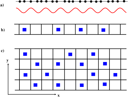
Figure 1: (Color online) Schematic pictures of the friction models and the Josephson junction array. a) the Frenkel-Kontorova (FK) model b) Matsukawa-Fukuyama’s 2-chain model on the ladder lattice and c) the Josephson junction array (JJA) on a square lattice under external magnetic field. The squares in the plaquette represent positions of the vortexes induced either by mismatching between the two incommensurate surfaces b) or external magnetic field c).

2.1 Frenkel-Kontorova model - starting point

2.1.1 Frustration due to mismatching

The original Frenkel-Kontorova model [12] is a one-dimensional elastic chain of particles put on a periodic substrate (see Fig. 1 a)). The Hamiltonian is given by,

$$H=\sum_{n=1}^{L}\left\{\frac{k}{2}(u_{n+1}-u_{n}-l)^{2}-\lambda\cos\left(\frac{\pi u_{n}}{a}\right)\right\}.$$ (1)

Here $u_{n}$ denotes the position of the $n$-th particle. The particles are connected to each other by Hookian springs of strength $k$ as described by the 1st term in the Hamiltonian where $l$ is the natural spacing between the particles. We impose a boundary condition such that the length of the whole system is fixed $(u_{L+1}-u_{1})/l=L$. The 2nd term describes the periodic potential due to the substrate whose period is $a$.

There are two important parameters: 1) the strength of the potential $\lambda$ and 2) winding number $f$,

$$f=\frac{l}{2a}.$$ (2)

Both are crucial for the jamming-unjamming transition (Aubry’s transition) in the FK model [10, 11]. Later we will find equivalent two parameters in the frustrated Josephson junction array under external magnetic field.

The sinusoidal potential allows the elastic chain to make phase slips with respect to the substrate. Thus this simple system allows both elastic and plastic deformations. The elastic term prefers to keep the natural spacing $l$ while the substrate potential prefers $2a$. In the context of the friction between two different materials brought in contact with each other [18], it is natural to suppose that the two surfaces are incommensurate with respect to each other, namely $f$ is an irrational number - a number which cannot be represented as a ratio of some two integers. As the result the system becomes frustrated as soon as $\lambda$ becomes finite. Finding the ground state of the system, which is some periodic (possibly of very long periodicity) crystalline structure for rational $f$, becomes a highly non-trivial problem [26]. In the present paper we always assume $f$ is irrational.

The system exhibits a jamming or frictional transition - called as Aubry’s transition [10, 11] which we review in section 3. For weak enough coupling $\lambda<\lambda_{c}$ the elastic chain is only mildly deformed and it can slide over the substrate smoothly without energy dissipation - friction-less. For stronger coupling $\lambda>\lambda_{c}$, the elastic chain becomes pinned by the substrate and friction emerges. We will find later that the parameter $\lambda$, which plays a key role in the FK model, is equivalent to strength of anisotropy of the Josephson coupling in the Josephson junction array.

2.1.2 Phase representation

It is convenient to introduce a dimension-less “phase” variable $\theta_{n}$ defined by $u_{n}=\frac{a}{\pi}[\theta_{n}+2\pi(f-1)n]$ by which the (dimension-less) Hamiltonian can be rewritten as,

$$H=\sum_{n=1}^{L}\left\{\frac{1}{2}(\theta_{n+1}-\theta_{n}-2\pi)^{2}-\lambda\cos(\theta_{n}+2\pi fn)\right\}$$ (3)

where $\lambda$ is also made dimension-less by an appropriate rescaling. The boundary condition is such that $(\theta_{L+1}-\theta_{1})/2\pi=L$ is fixed.

2.2 Matsukawa-Fukuyama model - a crucial intermediate step

2.2.1 Phase model on ladder-lattice

Matsukawa and Fukuyama considered a two-chain model in the context of friction [13]. Their idea is to allow the “substrate” in the FK model to deform elastically as well, which is certainly more realistic than the FK model in the context of tribology [18]. Following their idea, let us modify the FK model Eq. (3) and develop a phase model defined on a two-leg ladder lattice shown in Fig.1 b). The hamiltonian is given by,

$$H=\sum_{\vec{e}_{ij}=\vec{e}_{x}}\frac{1}{2}(\theta_{i}-\theta_{j}-2\pi)^{2}-\lambda\sum_{\vec{e}_{ij}=\vec{e}_{y}}\cos(\theta_{i}-\theta_{j}-2\pi fn_{i})$$ (4)

To simplify notations we relabeled the sites as $i=1,2,\ldots,N$ whose position in the real space is given by $(n_{i},m_{i})$. In the two-chain model the index for the column takes values $n=1,2,\ldots,L$ while that for the row (or layer) takes just two values $m=1,2$. The sums are took over nearest neighbour pairs connected by displacement vector $\vec{e}_{ij}=(n_{i}-n_{j},m_{i}-m_{j})$ which is either equal to $(1,0)$ or $(0,1)$.

2.2.2 Gauge invariance

An important property of the system is gauge invariance which we explain below. Let us rewrite the hamiltonian Eq. (4) as,

$$H=\sum_{\vec{e}_{ij}=(1,0)}\frac{1}{2}\psi^{2}_{ij}-\lambda\sum_{\vec{e}_{ij}=(0,1)}\cos(\psi_{ij})$$ (5)

with the phase difference

$$\psi_{ij}\equiv\theta_{i}-\theta_{j}-A_{ij}.$$ (6)

Here $A_{ij}$ is an anti-symmetric matrix $A_{ij}=-A_{ji}$ which satisfy,

$$\sum_{\rm plaquette}A_{i,j}=2\pi f.$$ (7)

The sum $\sum_{\rm plaquette}$ is a directed sum over “bonds” along each “plaquette” in the anti-clockwise manner.

It is easy to see that the original representation Eq. (4) respect the condition Eq. (7). The crucial point is that the phase differences $\psi_{ij}$ are invariant under gauge transformations;

$$\theta_{i}\to\theta_{i}+\delta\theta_{i}$$ (8)

$$A_{ij}\to A_{ij}+\delta\theta_{i}-\delta\theta_{j}$$ (9)

Thus the hamiltonian Eq. (4) is gauge-invariant. The condition Eq. (7) itself is also gauge-invariant.

In addition to the gauge invariance, the hamiltonian Eq. (5) is invariant under $A\to-A$ with $\theta_{n}\to-\theta_{n}$. Furthermore also $f\to 1+f$ does not change the problem. So we only need to consider $0<f\leq 1/2$ in the following.

2.3 Frustrated Josephson-junction array (JJA) under magnetic field

2.3.1 Frustration due to external magnetic field

The final step is just to 1) increase the number of legs of the ladder to build a 2-dimensional square lattice and 2) replace the intra-layer elastic couplings by sinusoidal couplings ((see Fig. 1 c)). Then we obtain the Josephson junction array on a square lattice under external magnetic field applied perpendicularly to the array [14],

$$H=-\sum_{\vec{e}_{ij}=(1,0)}\cos(\psi_{ij})-\lambda\sum_{\vec{e}_{ij}=(0,1}\cos(\psi_{ij})$$ (10)

Here $\theta_{i}$ is identified as the phase of the superconducting order parameter of the $i$-th site (superconducting island). The sinusoidal couplings represent Josephson coupling between the superconducting islands. Now the potential $A$ is identified as the vector potential due to external magnetic field $B_{z}$ applied along the $+z$ direction. The parameter $f$ which appears in Eq. (7) is the number density of quantized flux lines $f=a^{2}B_{z}/\phi_{0}$ where $a^{2}$,$B_{z}$ and $\phi_{0}$ are the are of the plaquette, strength of the magnetic and flux quantum.

Let us emphasize that the two important parameters in the FK model, namely 1) the parameter $\lambda$ and 2) the winding number $f$ are inherited down to the the JJA. To conclude we finally arrived a Josephson junction array on a square lattice with anisotropic coupling - with anisotropy $\lambda$ - under external magnetic field $B_{z}=(\phi_{0}/a^{2})f$ - with irrational number density $f$ of fluxes per plaquette. In short, let us call such a system as irrationally frustrated anisotropic JJA.

Quite interestingly it is actually possible to construct anisotropic JUL in laboratory. The strength of the Josephson coupling depends, for instance, on the thickness of the junctions. Saito and Osada [27] created anisotropic JJA with various $\lambda$ by controlling the thickness of the junctions in the lithography process.

It may sound rather strange to consider the anisotropy seriously since it usual plays only minor roles. Not surprisingly, previous studies of irrationally frustrated JJA considered only isotropic systems $\lambda=1$. As we discuss later, it turned out in our recent studied that $\lambda$ is actually relevant for irrational $f$ [5, 6, 7]. Quite remarkably the isotropic point $\lambda=1$ turned out to be a critical point at zero temperature corresponding to $\lambda_{c}$ of the FK model where a jamming transition analogous to the Aubry’s transition takes place. By symmetry it is obvious that we only need to consider the case $\lambda\geq 1$.

2.3.2 Vortex - analogue of dislocation

We mentioned above that the parameter $f$ can be regarded as number density of quantized flux lines per plaquette. As we explain below, this is because the vector potential $A$ due to the magnetic field induces vortexes of the phases $\theta_{i}$. The point is that vortexes are quantized objects like dislocations in crystals.

Here it is convenient to define “charges” of the vortexes as,

$$q_{i}=\frac{1}{2\pi}\sum_{\rm plaquette}s(\psi_{ij})=p_{i}-f\qquad p_{i}=\ldots,-2,-1,0,1,2,\ldots$$ (11)

where $s(x)$ is a saw-tooth like periodic function with period $2\pi$ and $s(x)=x$ in the range $-\pi<x\leq\pi$. By definition, the charge $q$ takes only discrete values of the form $p_{i}-f$ with some integer $p_{i}$ and offset $-f$ as shown above. Physically the integer $p_{i}$ represents the number of quantized fluxes (each carrying a flux quantum $\phi_{0}$) threading the $i$-th plaquette. Note also that the charge $q$ is gauge invariant.

The usefulness of the charge becomes manifested in the so called coulomb-gas mapping (see Chap. 9 of Chaikin-Lubensky) in which continuous, elastic deformations (“spin-wave”) are integrated out to find effective hamiltonian ${\cal H}$ of the vortexes. The resultant system is essentially equivalent to a lattice-gas of electrostatic charges interacting with each other by the repulsive coulomb interactions,

$${\cal H}=\sum_{i\neq j}q_{i}G(\vec{r}_{ij})q_{j}+G({\vec{0}})\sum_{i}q^{2}_{i}$$ (12)

with ${\vec{r}}_{ij}=(n_{i}-n_{j},m_{i}-m_{j})$.

The interaction potential $G({\vec{r}})$ is the (static) Green’s function of elastic deformations (spin-wave). In 2-dimension, it scales as $G({\vec{r}})\propto\log(|{\vec{r}}|)$ for $r\gg 1$. Note that the anisotropy $\lambda$ in Eq. (10) is simply reflected in anisotropy in $G({\vec{r}})$ such that with it is stronger into $y$-direction ${\vec{r}}||(0,1)$ compared to $x$-direction ${\vec{r}}||(1,0)$ by factor $\lambda(\geq 1)$.

The value $G({\vec{0}})(>0)$ can be interpreted as the core energy of the vortexes. Because of the core energy, states with higher values of the vortex charges generally have larger energies and can be neglected at low temperatures. Since we only need to consider $0<f\leq 1/2$ as noted in sec 2.2.2, it is sufficient to consider two values of the charges $q=-f,1-f$. In addition we assume the charge neutrality $\sum_{i}q_{i}=0$ holds, which can be enforced by applying the periodic boundary conditions. As the result we find that a fraction $f$ of the plaquettes carries a vortex $p=1$ (or $q=1-f$) and the other fraction $1-f$ carries no vortex $p=0$ ( or $q=-f$). In Fig. 1, the boxes in the plaquette represent the vortexes ($p=1$).

2.3.3 Vortex patterns in equilibrium - vortex liquid, crystal and glass

Let us sketch briefly possible patterns of vortexes in equilibrium states at low temperatures. For clarity we discuss three cases 1) $f=0$ 2) $f$ is rational and 3) $f$ is irrational.

If $f=0$, the ground state of the system is trivial: the phase becomes uniformly ordered $\theta_{i}={\rm constant}$ for all sites $i$. In such a ground state the vortex is absent everywhere $p_{i}=0$ ($q_{i}=0$). It can be regarded as a crystalline state (or ferromagnetic state). At finite temperatures, pairs of vortex ($p=1$) and anti-vortex ($p=-1$) will be created leading to melting of the crystalline state by proliferation of the vortexes (and anti-vortexes) at some critical temperature $T_{\rm c}$. In 2-dimension, it takes place in a special way named as Kosterlitz-Thouless transition [30].

If $f$ is rational, i. e. $f=p/q$ with some integers $p$ and $q$, the system will have a period vortex lattice [26], which is analogous to periodically ordered structure of dislocations in the so called Frank-Kasper phase [31]. For example with $f=1/2$, the charges exhibit a checkerboard like order in which the sign of the charges alternates along $x$ and $y$-axis as $q=1/2,-1/2,1/2,-1/2,\ldots$ (or $p=1,0,1,0,\ldots$). We also note that the ’half-vortexes’ which appears in the case of $f=1/2$ is identical to the so called chirality in frustrated magnets [32, 33].

In bulk superconductors formation of the vortex lattice is well known. The latter is a triangular lattice called as Abrikosov lattice [14]. On the other hand, the vortex lattices in JJA are formed on top of the underlying square lattice so that it is a super-lattice. Thus the vortex lattices in JJA are usually pinned by the underlying lattice of the JJA while those in the bulk pure superconductors are free to move around unless some pinning centers are present [25, 35].

Starting from the FK model we are naturally lead to consider irrational $f$. Apparently the system cannot develop simple periodic vortex lattices with irrational $f$ so that finding the ground state becomes a highly non-trivial problem. Indeed JJA with irrational $f$ - irrationally frustrated JJA - has been regarded as a system which possibly exhibit a glassy phase since a seminal work by T. Halsey [36]. This is a quite intriguing possibility since it means emergence of a glassy phase with frustration but without quenched disorder - at variance with the conventional spin-glasses and vortex-glasses (superconductors with random pinning centers) which involve quenched disorder [25, 35]. Disorder may be somehow self-generated in this system. Indeed equilibrium relaxations of the irrationally frustrated JJA were similar to the primary relaxation observed in typical fragile supercooled liquids [37].

3 Low lying states and Aubry’s transition

3.1 Hull function of the FK model

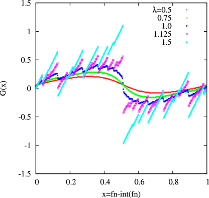
Figure 2: (Color online) Hull function $G(x)$ of the FK model. Here $\theta_{n}-2\pi n$ of the ground states are plotted against the “folded coordinate” $[n]=fn-{\rm int}(fn)$ to elucidate the hull function. $\lambda_{c}=0.9716..$ [11].

Now let us turn to review the Aubry’s transition found in the FK model[12, 10, 11, 38] and related friction models including the MF model [13, 39]. A remarkable feature of the FK model is that mathematically rigorous analysis of the low lying states is possible based on the fact that configuration of the energy minima (and maxima) of the system satisfies a recursion relation which is identical to the so called standard map well known in dynamical systems.

It is known rigorously that the ground state of the FK model can be expressed as[10, 11],

$$\theta_{n}=2\pi n+G(fn+\alpha)$$ (13)

where $G$ is a periodic function with periodicity $1$, i.e. $G(x+1)=G(x)$ for any $x$. The function $G(x)$ is called ’hull function’ and describes distortion of the configuration of the elastic chain due to the substrate potential. It is important to note that the entire region $0<x\leq 1$ becomes equally populated in the thermodynamic limit $L\to\infty$ for irrational $f$.

Quite remarkably the phase $\alpha$ is arbitrary, meaning that there is a manifold of ground states which have exactly the same energy. Moreover it is known rigorously that there is a “phase transition” for irrational $f$, called ’transition by breaking of analycity’ (or Aubry’s transition), at a critical strength of coupling $\lambda_{c}(f)$. The basic feature of the transition is summarized in the table 1. In Fig. 2 we show the hull function of the FK model constructed from numerically generated ground states at various $\lambda$ (see Ref [11] for the method).

	$G(x)$	(meta)stable states
$\lambda<\lambda_{c}(f)$	analytic	only the ground state
$\lambda>\lambda_{c}(f)$	non-analytic, with infinitely many discontinuities	infinitely many metastable states[38]

Table 1: Changes of the low lying states by the Aubry’s transition

From a physical point of view, a significant consequence of the Aubry’s transition is the “frictional transition” between the sliding phase and jamming (pinned) phase [11]. Let us sketch the essence of the reasoning in the following.

For $\lambda<\lambda_{c}$, starting from a ground state, one can find a continuum of states with exactly the same energy by varying $\alpha$. The point is that they are all related to each other by some continuous displacements of the particles in the real space. This comes from the fact that $G(x)$ is analytic for $\lambda<\lambda_{c}$. Thus no external force is needed to slide the whole system - friction-less or sliding.

Existence of the sliding becomes trivial if the elastic chain itself is replaced by a rigid body. In such an extreme case of friction between two incommensurate rigid bodies, the forces between them oscillates in the space with an incommensurate period so that the net force becomes cancelled out. The non-trivial point is that similar cancellation of the forces still happens even if the chain is allowed to deform elastically as long as the coupling $\lambda$ is sufficiently small.

For $\lambda>\lambda_{c}$, discontinuous points appear in the hull function $G(x)$. It means that variation of $\alpha$ require discontinuous movements of the particles in the real space. Thus the ground states are no-more connected to each other by sliding: the system prepared in the ground state has to go over some higher energy states (thus energy barriers) to reach another ground state. Thus the system is jammed. Now some finite strength of external force greater than a certain frictional force (yield stress) $f_{\rm yield}(\lambda)\propto(\lambda-\lambda_{c})^{\beta}$ must be applied to the system to let it move (de-pinning) [11].

Firov et al [38, 12] has been able to find a hierarchy of exponentially large number of low lying states on top of the ground state in the jammed phase $\lambda>\lambda_{\rm c}$. This is a very interesting observation from the view point of the physics of glasses. However, unfortunately the FK model is an one-dimensional system so that the Aubry’s transition disappears at finite temperatures.

The frictional transition and emergence of discontinuity in the hull function has also been found in the Matsukawa-Fukuyama’s 2-chain model [39]. Now it is very natural to expect that these features will be inherited down to our JJA on the square lattice under magnetic field. The main message that we find here is that we should vary the anisotropy $\lambda$ and see what happens in the low lying states.

3.2 Low lying states of the anisotropic JJA

Let us now turn to the anisotropic irrationally frustrated JJA with $\lambda>1$. Examples of the real space configurations of the vortexes in equilibrium at a low temperature are shown in Fig. 3. The most prominent feature is the stripe pattern of the vortexes which are regularly stacked into $y$-direction (stronger coupling) and undulated along the $x$-direction (weaker coupling) [5, 6, 7]. The formation of the stripes is reasonable because the repulsive interactions between vortexes are anisotropic if $\lambda\neq 1$ as we noted in sec 2.3.2.

There are two important observations. First, the undulated stripe pattern is frozen in time, i. e. the ergordicity is broken. The pattern of the undulation cannot evolve dynamically by usual relaxational dynamics once such a structure is established. This is simply because the stripes are perfectly stacked into the $y$-direction in a belt. At a first sight, the stripe patterns may look similar to those found, for example, in liquid crystals. But they are very different because usual stripes fluctuate dynamically [29].

Second, there is a family of low lying states with different patters of the transverse undulation as shown in Fig. 3. Apparently the ground state should have no transverse undulation. Very interestingly the energies of the different patterns of the undulation shown in Fig. 3 are very close to each other suggesting a gap-less band of undulated states. Thus these undulated states are all relevant in the equilibrium ensemble. This is manifested in the structure factor of the vortexes which exhibit Bragg peaks into $q_{y}$ direction but a power law tail into $q_{x}$ direction [6, 7].

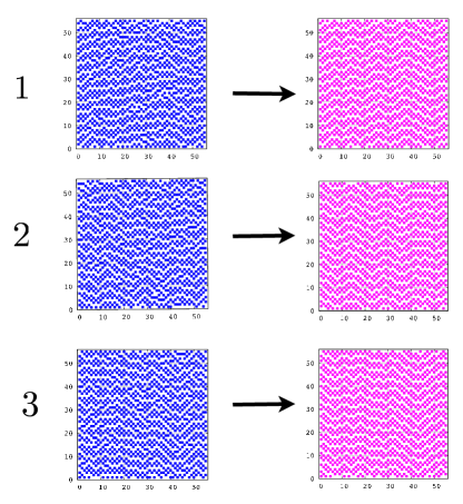
Figure 3: (Color online) Undulated vortexes in the anisotropic irrationally frustrated JJA. a) Examples of real space patterns of vortexes in thermal equilibrium at a low temperature and b) in nearby energy energy minima. The thermalized configurations shown in a) are obtained by performing Monte Carlo (MC) simulations at $T=0.2$ on a system with $f=21/55$ and $\lambda=1.5$. The equilibration is extremely hard in this system so that we used a MC method which combines the Metropolis method, over-relaxation method and exchange MC method to endure equilibration [40]. The filled squares represent plaquettes with vortexes with charge $p=1$. The configurations in b) are obtained by minimizing the energy by simple energy descent algorithm starting from the thermalized configurations shown in a). The energies of the energy minima of the configurations 1)-3) are $E=-5072.14311,-5072.38582,-5072.34445$ respectively.

This is a very peculiar state of matter. Is this a glass? “No”, in the sense that it has Bragg peaks which one would not expect for a glass. “Yes”, in the sense that there are many states with different patterns of undulation, which is a self-induced disorder, and they are separated by energy barriers.

In a sense, the prediction by Halsey [36] - that superconducting glass (without quenched disorder) in the JJA with irrational $f$ - is realized. However we must keep in mind that here we are considering anisotropic JJA with $\lambda>1$ instead of the isotropic JJA $\lambda=1$ studied in most of the previous works.

Now let us examine the low lying state more closer. In the analysis of the ground state of the FK model, the hull function Eq. (13) played a central role as we noted before. Since the JJA can be regarded as a 2-dimensional version of the FK model, we are naturally led to look for similar one which may describe the low lying sates of the JJA in a compact way.

Because of the gauge invariance, let us focus on the gauge-invariant phase differences across the Josephson couplings $\psi_{ij}=\theta_{i}-\theta_{j}-A_{ij}$ defined Eq. (6) where $i$ and $j$ are nearest neighbours across a Josephson coupling which may be either along $x$ or $y$-axis. As we discuss later $\psi_{ij}$ is directly related to the Josephson current $\sin(\psi_{ij})$, which is the analogue of stress field in rheology.

In Fig. 4 we display the phase differences $\psi_{ij}$ at various sites $i=(n,m)$ plotted against “folded coordinates” $[n]=fn-{\rm int}(fn)$ and $[m]=fm-{\rm int}(fm)$ which takes values limited in the range $0<[n]\leq 1$ and $0<[m]\leq 1$. The purpose of this plot is to elucidate the hull function analogously to the case of the FK model shown in Fig. 2. Quite remarkably the plots in the panels c) and d) strongly suggest there is indeed an analytic hull function of the folded coordinate along the direction of stronger coupling. On the other hand, the panels a) and b) suggest there are no such analytic hull functions along the direction of weaker coupling.

Recently we found it is possible to obtain the hull functions analytically by performing a $1/\lambda$ expansion starting from $\lambda=\infty$ limit [7]. It turned out that the transverse undulation is encoded in the “phase differences” between different columns which one can see in the pane-ll c) and d).

The existence (absence) of analytic hull functions along stronger (weaker) couplings immediately implies sliding (jamming) of the vortexes. Starting from an energy minimum, a family of different states with exactly the same energy can be obtained through the operation $[m]\to[m+\alpha]$ along the direction of stronger coupling with varying phase shift parameter $\alpha$. This amount to a unidirectional motion of the undulated vortex stripes into the direction of stronger coupling without changing its pattern, i. e. sliding. In contrast, no such operation is possible along the direction of weaker coupling, i. e. jamming. In the next section we discuss how these properties are reflected in physical observables associated with shear.

The above observation implies the symmetric system with $\lambda=1$, on which most of the previous works have been dedicated, is actually very special. As we discuss later, the critical point corresponding to the Aubry’s transition point is actually $\lambda_{c}=1$ in the JJA at zero temperature $T=0$.

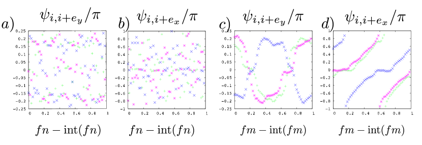
Figure 4: (Color online) Spatial configuration of gauge invariant phases in an energy minimum. Phase differences $\psi_{i,i+e_{x}}$ and $\psi_{i,i+e_{y}}$ across Josephson junctions parallel to $x$ and $y$ axes at various sites $i=(n,m)$ are plotted against “folded coordinates”. Different symbols in the panels a) and b) represent the phase differences at $n=1,2,\ldots,L$ along arbitrary chosen three different “rows” of the JJA. In the panels c) and d), the phase differences at $m=1,2,\ldots,L$ along arbitrary chosen three “columns” are shown. The system size is $L=55$.

4 Response to shear - shear by external electric current

Jamming is nothing but onset of rigidity which can be detected by response against shear. In general shear is induced into the system through the boundaries. In rheology one can consider to apply some constant external shear-stress $\sigma_{\rm ext}$ on boundaries of systems under study. Very interestingly this is equivalent to put external electric current $I_{\rm ext}$ into a Josephson junction array as we explain in sec 4.2. We will find that stress $\sigma$ and shear rate $\dot{\gamma}$ in rheology correspond precisely to current $I$ (or current density $J$) and voltage $V$ (or electric field $E$) in the transport problem of the driven JJA.

To study rheology (or transport) one can control either the external stress $\sigma$ or shear rate $\dot{\gamma}$. Here we choose to control the strain $\gamma$ so that we can discuss static and dynamic response to shear in the same set up.

We put shear across the Josephson junction array along, say $y$-axis, in the following manner. First we fix the configurations of the phase variables $\theta_{i}$ on the bottom ($m=1$) and top ($m=L$) layers. Second we slightly change the boundary such that a uniform displacement is imposed on the top layer ($m=L$) $\theta_{i}\to\theta_{i}+(L-1)\gamma$ while the bottom layer ($m=1$) is left in the same fixed configuration. This amount to induce a gradient of phase $d\theta/dy=\gamma$ along the $y$-axis. Clearly $\gamma$ corresponds to shear-strain of the usual sense. As the result some internal stress $\sigma$, which is super-current running across the Josephson junctions (see below), will be induced in the system. To study rheology, we drive the top wall with a constant speed so that the strain $\gamma$ increase with a constant shear-rate $\dot{\gamma}$. Let us also remark that shear $d\theta/dy=\gamma$ on the phases along the $y$-axis amount to motion of vortexes (dislocations) into the orthogonal direction, i.e. $x$-axis. This is equivalent to say that the vortexes are driven by the Lorentz force [14].

4.1 Static response to shear - static rigidity

From static point of view, emergence of rigidity can be best quantified by shear-modulus. The free-energy of the system $F(\gamma)$ can be formally expanded in power series of infinitesimal shear strain $\gamma$ as

$$F(\gamma)=F(0)+N\langle\sigma\rangle\gamma+\frac{N}{2}\mu\gamma^{2}+\ldots$$ (14)

where $\sigma$ and $\mu$ are the shear-stress and shear-modulus respectively. $\langle\ldots\rangle$ stands for a thermal average.

Here $\gamma$ must be infinitesimal. The free-energy density $F(\gamma)/N$, in the thermodynamic sense, must not depend on the boundary condition (including the shape of the container) so that shear-modulus must be zero in the thermodynamic sense even in solids. Thus when the shear-modulus $\mu$ defined by the fluctuation formula Eq. (17) emerges, it means that the ordering of the $\gamma\to 0$ limit and the thermodynamic limit $N\to\infty$ no more commute in sharp contrast to liquids. In turn this means linear elasticity must fail in solids. Physically this means that elasticity and plasticity must emerge simultaneously in solids.[42]

It is useful to note that the change on the boundary condition can be formally “absorbed” into the bulk part of the system by replacing the original Hamlitonian Eq. (10) by,

$$H(\gamma)=-\sum_{\vec{e}_{ij}=(1,0)}\cos(\psi_{ij})-\lambda\sum_{\vec{e}_{ij}=(0,1)}\cos(\psi_{ij}+\gamma).$$ (15)

Based on this observation we find that the stress $\sigma$ can be expressed as,

$$N\sigma=\frac{\partial H(\gamma)}{\partial\gamma}=\lambda\sum_{\vec{e}_{ij}=(0,1)}\sin(\psi_{ij}).$$ (16)

Similarly the shear-modulus $\mu$ can be expressed as,

$$\mu=b-\beta\left[\langle\sigma^{2}\rangle-\langle\sigma\rangle^{2}\right]$$ (17)

where $b$ is instantaneous or adiabatic shear-modulus (“Born term”) defined as,

$$Nb=\frac{\partial^{2}H(\gamma)}{\partial\gamma^{2}}=\lambda\sum_{\vec{e}_{ij}=(0,1)}\cos(\psi_{ij}).$$ (18)

Fluctuation formulae for the elastic modulus like Eq. (17) are well known in literature [41]. In the context of XY models and super-conductors it is usually called as helicity modulus [29]. The crucial term is the 2nd term which represents reduction of the shear-modulus due to thermal fluctuations of the stress $\sigma$.

In liquids, the two limits $\gamma\to 0$ and $N\to\infty$ should commute. Then an identity $\mu=0$ must hold meaning exact cancellation must take place between the Born term and the fluctuation term in Eq. (17).

In the previous section we found the anisotropic irrationally frustrated JJA exhibits sliding/jamming in the low lying states such that the vortexes can slide freely along the stronger coupling but jammed along the weaker coupling. In turn this means that shear of the phases along stronger/weaker coupling causes finite/zero changes of the energy respectively. Consequently the shear-modulus $\mu$ must be finite/zero along stronger/weaker coupling at zero temperature $T=0$. Indeed we observed this numerically [5].

This is a quite intriguing situation - the anisotropic system $\lambda\neq 1$ at zero temperature $T=0$ behaves either as solid or liquid depending on the axes along which one imposes the shear. From numerical observations it seems that the picture holds up to the symmetric point $\lambda=1$ [5] suggesting that the symmetric point is actually the critical point $\lambda_{c}=1$ where shear-modulus along a given axis becomes zero/finite.

4.2 Dynamic response to shear - transport or rheology

The shear-stress $\sigma$ defined in Eq. (16) is nothing but super-current flowing along $y$-direction in the Josephson junction array. More precisely according to the DC/AC Josephson relations [14] the current $I_{ij}$ and voltage drop $V_{i}-V_{j}$ across the junction are given by,

$$I_{ij}=\sin(\psi_{ij})\qquad V_{i}-V_{j}=\frac{d\psi_{ij}}{dt}$$ (19)

Here we are assuming some appropriate rescalings to define the dimension-less quantities $I_{ij}$ and $V_{i}$.

At each site $i$ (super-conducting island) the current must be conserved. By taking into account charging of the island and Ohmic energy dissipation we find,

$$C\frac{dV_{i}}{dt}+\sum_{j}\frac{V_{i}-V_{j}}{R}+\sum_{j}I_{ij}=I_{\rm ext}(\delta_{m_{i},L}-\delta_{m_{i},1})$$ (20)

where the sums are took over nearest-neighbours. $C$ and $R$ are the capacitance of the islands and resistance of the junctions respectively. $I_{\rm ext}$ is the strength of external current which is injected from the top layer $m=L$ and extracted from the bottom layer $m=1$. Combining with the Josephson relation Eq. (19) and the definition of the gauge-invariant phase difference $\psi_{ij}$ given in $Eq.~{}(\ref{eq-def-psi})$, one easily finds an effective equation of motion of the phases $\theta_{i}$, which is called RCSJ (Resistively and Capacitively Shunted Junction) model[14]. Apparently it can be cast into the form of Newton’s equation of motion,

$$\frac{d\theta_{i}}{dt}=v_{i}\qquad m\frac{dv_{i}}{dt}+\frac{\partial H}{\partial\theta_{i}}+\eta\sum_{j}(v_{i}-v_{j})=F_{\rm ext}(\delta_{m_{i},L}-\delta_{m_{i},1}).$$ (21)

which can be considered as a toy model for rheology of layered systems under external shear applied on the top and bottom walls [17].

From the above observations, it is clear that transport properties in JJA and rheology are quite analogous. Because of the shear, the velocity field $d\theta_{i}/dt$ will acquire a slope along the $y$-axis which can be identified with the shear rate $\dot{\gamma}$. From the AC Josephson relation (the 2nd equation of Eq. (19)), we find that it mounts to a constant electric field $E$ along the $y$ axis.

To summarize shear-stress $\sigma$ and shear-rate $\dot{\gamma}$ in rheology correspond to electric current $I$ (or current density $J$) and voltage drop $V$ across the system (or electric field $E$) in the transport problem of JJA. Thus the so called “flow curves” in rheology corresponds to current-voltage $IV$ (or $JE$) characteristics in JJA. In tribology we just need to consider only two layers $m=1,2$ as in the Matsukawa-Fukuyama’s 2-chain model [13]. The yield stress $\sigma_{\rm c}$ is called as static frictional force. These problems have been studied extensively in the corresponding research communities but somehow the intimate analogy has not been appreciated [17].

4.3 Non-linear rheology and transport

Let us discuss here some basic phenomenological aspects of the non-linear rheology and the non-linear transport associated with 2nd order phase transition, including the jamming transition. To be specific we will denote $\lambda-\lambda_{c}$ as the distance to the critical point which is natural in the context of the anisotropic JJA at zero temperature. However the readers can easily translate the discussion to different situations by replacing $\lambda-\lambda_{c}$ by distance to critical temperature $T-T_{c}$ or jamming density $\phi-\phi_{\rm J}$, e.t.c. depending on the problems at hand.

Let us assume the following generic scaling form.

$$\sigma=|\lambda-\lambda_{c}|^{\beta}\tilde{\sigma}_{\pm}\left(\frac{\dot{\gamma}}{|\lambda-\lambda_{c}|^{\Delta}}\right)$$ (22)

where $\beta$ and $\Delta$ are critical exponents and the subscript $\pm$ stands for $\lambda>\lambda_{c}$ and $\lambda<\lambda_{c}$ respectively. Physically we expect the following behaviours: 1) Newtonian behaviour in the “sliding phase” ($\lambda<\lambda_{c}$), 2) Finite yield stress in the “jammed phase” ($\lambda>\lambda_{c}$) and 3) The explicit $\lambda$ dependence must disappear at the critical point ($J$-point) $\lambda=\lambda_{c}$. Based on these intuitions let us conjecture the following asymptotic behaviours of the scaling function $\tilde{\sigma}(y)$,

$$\tilde{\sigma}_{\pm}(y)=\left\{\begin{array}[]{ll}\left\{\begin{array}[]{cl}y&\lambda<\lambda_{c}\\ \tilde{\sigma}_{-}(0)&\lambda>\lambda_{c}\end{array}\right.&y\ll 1\\ &\\ cy^{\beta/\Delta}&y\gg 1\end{array}\right.$$ (23)

where $\tilde{\sigma}(0)$ and $c$ are some constants. Consequently the scaling ansatz predicts the following asymptotic behaviours ($\dot{\gamma}\to 0$),

$$\lim_{\dot{\gamma}\to 0}\sigma=\left\{\begin{array}[]{lll}\eta(\lambda)\dot{\gamma}&\eta(\lambda)\propto(\lambda_{c}-\lambda)^{-(\Delta-\beta)}&\lambda<\lambda_{c}\\ c\;\dot{\gamma}^{\beta/\Delta}&&\lambda=\lambda_{c}\\ \sigma_{c}(\lambda)&\sigma_{c}(\lambda)=\tilde{\sigma}_{-}(0)(\lambda-\lambda_{c})^{\beta}&\lambda>\lambda_{c}\end{array}\right.$$ (24)

Most importantly the power law fluid behavior $\sigma\propto\dot{\gamma}^{\beta/\Delta}$ at the critical point is predicted. Usually $\beta/\Delta<1$ which is called shear-thinning behaviour.

For the transport problems in superconductors including JJA, one just need to replace shear-stress $\sigma$ by the electric current density $J$, shear-rate $\dot{\gamma}$ by the electromagnetic field $E$. The Newtonian law corresponds to the Ohmic law $J=\sigma E$ with the linear conductivity $\sigma$ and the yield stress $\sigma_{c}$ corresponds to critical current $J_{c}$.

Recently the non-liner rheology of granular systems is found to obey this type of scaling around the J-point [20, 21, 22, 23, 24]. In granular systems Bagnold’s scaling must replace the Newtonian law in the unjammed phase. At least formally, the above argument can be easily modified to account for it.

The above scaling ansatz is quite reminiscent of the scaling property of magnetization of ferromagnetic models around the critical temperature $T_{c}$. On purpose we actually used the same standard notations for the critical exponents, i. e. $\beta$ and $\Delta$, in the latter problem. Namely by replacing the stress $\sigma$ by magnetization $m$ and strain rate $\dot{\gamma}$ by magnetic field $h$, one recovers $m\propto|T-T_{c}|^{\beta}\tilde{m}_{\pm}(h/|T-T_{c}|^{\Delta})$. One can easily find precise correspondences between 1) the Newtonian (Ohmic) law v.s. paramagnetic behaviour $m=\chi h$ with the linear-susceptibility $\chi$ diverging at $T_{c}$ 2) power law rheology $\sigma\propto\dot{\gamma}^{\beta/\Delta}$ v.s. $m\propto h^{\delta}$ with $\delta=\beta/\Delta$ at the critical points and 3) yield stress (critical current) $\sigma_{c}\propto(\lambda-\lambda_{c})^{\beta}$ v.s. the spontaneous magnetization $m_{s}\propto(T_{c}-T)^{\beta}$.

This type of scaling has been advocated first in the context of non-linear current-voltage characteristics of superconductors by Wolf, Gubser and Imry [43]. They studied non-linear current-voltage characteristics of superconducting film at the superconducting phase transition, which is a Kosterlitz-Thouless type 2nd order phase transition[30]. They pointed out the analogy with the scaling of the magnetization of ferromagnets. Such dynamical scaling ansatz has been extensively used in the studies of transport properties in high-$T_{\rm c}$ superconductors, especially in the context of the vortex-glasses with quenched pinning centers [25].

More recently Otsuki and Sasa [20] has realized the same type of critical behavior in the context of the non-linear rheology of molecular glasses. Quite remarkably they were able to find a mean-field theory which predicts that the flow curves of the non-linear rheology are formally identical to the equation of state of the Landau-Ginzburg theory of ferromagnets under external magnetic field suggesting in particular $\beta/\Delta=1/3$.

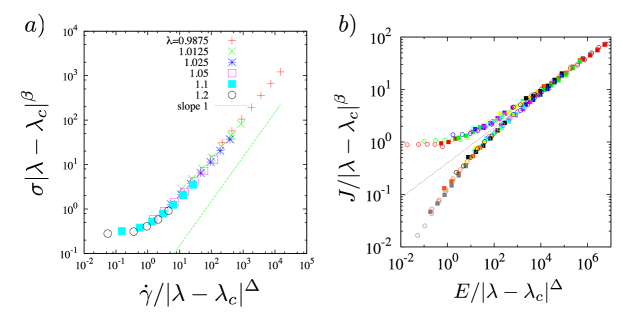
Figure 5: (Color online) Flow curves of the FK model and JJA. Both models are simulated by the RCSJ method at zero temperature $T=0$. The panel a) displays the master flow curve of the FK model using $\lambda_{c}=0.9716$..and $\beta=\Delta=3$. The panel b) displays the master flow curve of the irrationally frustrated anisotropic JJA using $\lambda_{c}=1$, $\beta=1.19$ and $\Delta=3.5$ so that $\beta/\Delta=0.34$.

Let us now discuss the dynamical scaling properties of the FK model and the JJA under shear. We performed the RCSJ simulation on both models. The master flow curve of the FK model is displayed in the panel a) of Fig. 5 which follow well the expected dynamical scaling behaviour around the Aubry’s transition point $\lambda_{c}$. A previous work [11] found $\sigma_{c}\propto(\lambda-\lambda_{c})^{\tilde{\psi}}$ with $\lambda_{c}=0.9716..$ and $2.85<\tilde{\psi}<3.06$. In addition we found the system remains Newtonian for the entire sliding phase $\lambda\leq\lambda_{c}$ including the critical point so we assumed $\beta=\Delta$ in the scaling plot.

For the irrationally frustrated anisotropic JJA, we pointed out in sec 4.1 that the shear-modulus $\mu$ along stronger/weaker coupling is finite/zero at zero temperature $T=0$ and that the symmetric point $\lambda_{c}=1$ is the critical point where the shear-modulus $\mu$ along a given axes changes from finite/zero to zero/finite. Then it is quite natural to expect that the current-voltage curve of the system with respect to injection of the electric current along a given direction exhibit dynamical scaling feature at around $\lambda_{c}=1$. This is indeed observed by a numerical simulation of the RCSJ dynamics [5]. The current-voltage curves collapse onto a master curves as shown in the panel b) of Fig. 5.

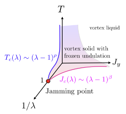
Figure 6: (Color onlie) ”Jamming” phase diagram of the JJA

4.4 Jamming phase diagram

In Fig. 6 we show a schematic “jamming phase diagram” of the irrationally frustrated anisotropic Josephson junction array. So far we discussed only the properties of the system at zero temperature $T=0$ and $\lambda\geq 1$. Under the electric current $J_{y}$ injected along the $y$-axis, the system remains jammed as long as $J_{y}$ is smaller than the critical current $J_{\rm c}\sim(\lambda-1)^{\beta}$. The configuration of the jammed solid phase is characterized by the frozen pattern of the undulated vortex stripes. Under strong enough current $J_{y}>J_{\rm c}$, the system starts to move exhibiting the shear-thinning behaviour. On the other hand the same solid can slide freely with respect to electric current $J_{x}$ injected along the $x$-axis for the entire $\lambda>1$ region. For the region $\lambda<$, we just need to interchange the $x$ and $y$-axes in the above discussion.

Previous studies on the irrationally frustrated JJA are almost exclusively concerned with the symmetric point $\lambda=1$. Recent intensive numerical studies at finite temperatures suggest $T_{c}(\lambda=1)=0$ [44, 45] without finite temperature glass transition anticipated in the early works [36, 37]. On the other hand our recent studies on the static properties at low temperatures [6, 7] strongly suggest $T_{c}(\lambda)>1$ at least sufficiently away from the symmetric point $\lambda=1$ and that $T_{c}(\lambda)$ rapidly decreases approaching the symmetric point $\lambda=1$. These point toward the possibility of the jamming phase diagram depicted in Fig 6. Quite interestingly it is very similar to the jamming phase diagram proposed by the Chicago group [8, 9]. Most notably the point $(\lambda=1,T=0)$ look quite similar to the Jamming point which deserves further studies.

5 Conclusions

To conclude we discussed static and transport or rheological properties of the irrationally frustrated anisotropic Josephson junction array (JJA) which exhibits vortex stripes with self-generated randomness at low temperatures. We emphasized in particular the intimate connection between the friction models and the irrationally frustrated JJA which provides valuable insights into the problems.

References

- [1] ”Jamming and Rheology: Constrained Dynamics on Microscopic and Macroscopic Scales”, Ed. A. J. Liu , S. R. Nagel, CRC Press (2001).
- [2] J. Kurchan and D. Levine, arXiv:0904.4850v1.
- [3] Geometrical frustration, J. F. Sadoc, Rémy Mosseri, Cambridge University Press, (1999).
- [4] G. Tarjus, S. A. Kivelson, Z. Nussinov and P. Viot, J. Phys. Condens. Matters 17 (2005) R 1143 .
- [5] H. Yoshino, T. Nogawa and B. Kim, New J. Phys. 11 (2009) 013010.
- [6] H. Yoshino, T. Nogawa and B. Kim, arXiv:0907.3763v1.
- [7] H. Yoshino, T. Nogawa and B. Kim, arXiv:1004.0585.
- [8] A. J. Liu and S. R. Nagel, Nature, Volume 396, Issue 6706, (1998) 21.
- [9] C. S. O’Hern, L. E. Silbert, A. J. Liu and S. R. Nagel, Phys. Rev. E 68, (2003) 011306.
- [10] S. Aubry, P. Y. Le Daeron, Physica D: Nonlinear Phenomena 8 (1983) 381.
- [11] M. Peyrard and S. Aubry, J. Phys. C: Solid State Phys. 16 (1983) 1593.
- [12] For a review see, ”The Frenkel-Kontorova Model - Concepts, Methods and Applications”, O. M. Braun and Y. S. Kivshar, Springer (2004).
- [13] H. Matsukawa and H. Fukuyama, Phys. Rev B. 49 (1994) 17286.
- [14] Introdunction to Superconductivity, M. Tinkham, Courier Dover Publications (2004).
- [15] H. S. J. van der Zant, H. A. Rijken, and J. E. Mooij, J. Low. Temp. Phys. 82 (1991) 67 and references there-in.
- [16] P. Martinoli and Ch. Leemann, J. Low Temp. Phys. 118 (2000) 699.
- [17] H. Yoshino, H. Matsukawa, S. Yukawa and H. Kawamura, J. Phys.: Conf. Ser. 89 (2007) 012014.
- [18] Physics of sliding friction, ed. B.N.J. Persson and E. Tosatti, Kluwer Academic Publishers, (1996).
- [19] ”Rheology: Principles, Measurements, and Applications”, C. W. Macosko, VCH (1994) New York.
- [20] M. Otsuki and S.-i. Sasa, J. Stat. Mech., (2006) L10004.
- [21] T. Hatano, M. Otsuki and S. Sasa, J. Phys. Soc. Jpn. 76 (2007) 023001.
- [22] P. Olsson and S. Teitel, Phys. Rev. Lett. 99 (2007) 178001.
- [23] T. Hatano, J. Phys. Soc. Jpn. 77 (2008) 123002 .
- [24] M. Otsuki and H. Hayakawa, Prog. Theor. Phys. 121 (2009) 647.
- [25] D. S. Fisher, M. P. A. Fisher and D. A. Huse, Phys. Rev. B 43 (1991) 130.
- [26] T. C. Halsey, Phys. Rev. B 31 (1985) 5728; P. Gupta, S. Teitel, and M. J. P. Gingras, Phys. Rev. Lett. 80 (1998) 105; C. Denniston and C. Tang, Phys. Rev. B 60 (1999) 3163.
- [27] S. Saito and T. Osada, Physica B: Condensed Matter Vol 284-288 (2000) 614.
- [28] C. Denniston and C. Tang, Phys. Rev. Lett. 75 (1995) 3930.
- [29] Principles of condensed matter physics, P. M. Chaikin and T. C. Lubensky, Cambridge University Press (1995).
- [30] J. M. Kosterlitz and D. J. Thouless, J. of Phys. C: Solid State Phys. 6 (1973) 1181.
- [31] F. C. Frank and J. S. Kasper, Acta Crystallogr. 11 (1958) 184; 12 (1959) 483.
- [32] J. Villain, J. of Phys. C: Solid State Phys., 10 (1977) 4793.
- [33] S. Teitel and C. Jayaprakash, Phys. Rev. B 27 (1983) 598.
- [34] S. Teitel and C. Jayaprakash, Phys. Rev. Lett. 51 (1983) 1999.
- [35] G. Blatter, M. V. Feigel’man, V. B. Geshkenbein, A. I. Larkin and V. M. Vinokur, Rev. Mod. Phys. 66 (1994) 1125.
- [36] T. C. Halsey, Phys. Rev. Lett. 55 (1985) 1018.
- [37] B. Kim and S. J. Lee, Phys. Rev. Lett. 78 (1997) 3709, S. J. Lee, B. Kim, and J. -R. Lee, Phys. Rev. E 64 (2001) 066103.
- [38] O.V. Zhirov, G. Casati and D. L. Shepelyansky, Phys. Rev. E 65 (2002) 26220.
- [39] T. Kawaguchi and H. Matsukawa, Phys. Rev. B 56 (1997) 13932.
- [40] K. Hukushima and K. Nemoto, J. Phys. Soc. Jpn 65 (1996) 1604, M. Creutz, Phys. Rev. D 36 (1987) 515.
- [41] D. R. Squire, A. C. Holt, and W. G. Hoover, Physica, 42, Issue 3, (1969) 388.
- [42] H. Yoshino and M. Mézard, arXiv:1003.3039.
- [43] S. A. Wolf, D. U. Gubser and Y. Imry, Phys. Rev. Lett. 42 (1979) 324 .
- [44] S. Y. Park, M. Y. Choi, B. J. Kim, G. S. Jeon, and J. S. Chung, Phys. Rev. Lett. 85 (2000) 3484.
- [45] E. Granato, Phys. Rev. Lett. 101 (2008) 027004.