The influence of electron density gradient direction on gradient-drift instabilities in the E-layer of the ionosphere

Abstract

We show that the dispersion relation for gradient-drift and Farley-Buneman instabilities within the approximation of the two-fluid MHD should contain the terms which are traditionally supposed to be small. These terms are caused by taking into account divergence of particles velocity and electron density gradient along the magnetic field direction. It is shown that at heights below 115km the solution of the dispersion relation transforms into standard one, except the situations, when the electron density gradient is parallel to magnetic field or wave-vector. In these cases the traditionally neglected summands to the growth rate of the irregularities becomes significant.

The additional terms depend on relative directions of electron density gradient, magnetic field and mean velocities. This leads to the different instability growth conditions at equatorial and high-latitude regions of the ionosphere. The obtained results do not contradict with the experimental data.

1 Introduction

In the recent review [Farely,2009] the equatorial instabilities at E-layer heights was analyzed, and the following problem was formulated: ”How different are the auroral and equatorial zones? Is the physics essentially the same, except for the fact that the auroral zone electric fields are often much stronger? Or is it important that in the auroral zone there are gradients parallel to the magnetic field in electron density, electron and ion temperatures and collision frequencies?”. In this paper we try to answer to this question.

As stated in [Farely,2009], the analysis of gradient-drift instabilities in the ionospheric plasma at E-layer heights in linear approximation is based on the theory suggested in [Fejer et al.,1975]. The result of the work [Fejer et al.,1975] is the correct derival of the dispersion relation for the plasma instabilities in the specific case when electron density gradient is oriented vertically, magnetic field - horizontally, electrons are magnetized and ions are unmagnetized. In the work [Fejer et al.,1975] authors also retrieved the well known solution of the dispersion relation. The attempt of solving the wider problem, when electron density gradients and magnetic field have arbitrary directions, was made in [Fejer et al.,1984] and is thought to be valid both for equatorial and high-latitude ionosphere. Unfortunately in the both papers the solution of the dispersion relation was obtained under a number of additional assumptions. Due to this fact these theories sometimes do not absolutely correctly describe the conditions of the instabilities generation, especially when the instabilities wave-vector or magnetic field are almost parallel to electron density gradient, as mentioned in [Farely,2009]. The possible cause of these problems is preliminary simplification of the dispersion relation and neglection of important terms.

The goal of the paper is the analysis of the dispersion relation solution, generalizing the formulas obtained in [Fejer et al.,1975, Fejer et al.,1984] by taking into account some terms traditionally neglected. We base on the same two-fluid magnetohydrodynamics (MHD) approximation as used in [Fejer et al.,1975] and assume that this approximation is valid for the heights under investigation. We use approach suggested in [Gershman,1974, Gelberg,1986] for studying the polar ionosphere. Then we investigate all the terms in the obtained solution to take into account important ones.

2 Solution of dispersion relation

2.1 Traditonal approach

The instability growth condition in presence of arbitrary direction of electron density gradient and electric and magnetic fields in linear approximation is retrieved, for example, in [Fejer et al.,1984]. The dispersion relation obtained there has a form:

$$\left(\omega+i2\alpha N_{0}-{\bf V_{d}}{\cdot}{\bf k}\right)\left(\nu_{in}-i\left(\omega-\frac{{\bf k_{\bot}}{\cdot}\left({\bf\nabla}N\times{\bf b}\right)\Omega_{i}}{k_{\bot}^{2}N}\right)\right) +$$

$$\left(\left(\omega+i2\alpha N_{0}\right)\left(\Omega_{i}^{2}+\left(\nu_{in}-i\omega\right)^{2}\right)+ik^{2}C_{s}\left(\nu_{in}-i\omega+i\frac{{\bf k_{\bot}}{\cdot}\left({\bf\nabla}N\times{\bf b}\right)\Omega_{i}}{k_{\bot}^{2}N}\right)\right)\cdot$$ (1)

$$\left(\frac{\Psi}{\nu_{in}}-i\frac{{\bf k_{\bot}}{\cdot}\left({\bf\nabla}N\times{\bf b}\right)\Omega_{i}}{k_{\bot}^{2}N}\right) =0$$

where ${\bf V}_{d}={\bf V}_{e0}-{\bf V}_{i0}$ - relative electron/ion drift velocity; $C_{s}=\sqrt{\frac{T_{e}+T_{i}}{m_{i}}}$ - ionacoustic speed, $\alpha$ - recombination coefficient;

$$\Psi=\frac{\nu_{en}\nu_{in}}{\Omega_{e}\Omega_{i}}\left(1+\frac{\Omega_{e}^{2}k_{||}^{2}}{\nu_{en}^{2}k^{2}}\right)$$ (2)

- a coefficient defining the aspect sensitivity of the instabilities, ${\bf b}=\frac{{\bf B}}{B}$.

To emphasize the problem of the dispersion relation (1), let us analyze a special case, when electron density gradient is parallel to the wave-vector and perpendicular to the magnetic field. In this case we have

$${\bf k_{\bot}}{\cdot}\left({\bf\nabla}N\times{\bf b}\right)=0$$ (3)

and in the standard dispersion relation (1) the presence of gradients can be neglected, and gradient-drift generation mechanism stop working.

The condition (3) is almost valid for non-disturbed equatorial ionosphere (where electron density gradient and wave vector are almost vertical), and for non-disturbed high-latitude ionosphere (where electron density gradient and magnetic field are almost vertical), so this problematic situation should arise frequently.

But sometimes this contradicts with the experimental data, for example at Earth magnetic equator, with vertical gradient of electron density and vertical wave-vector of sounding wave (and vertical wave-vector of irregularities, correspondingly) a powerful scattering is observed, as stated in [Farely,2009, pp.1515-1516]. This allows us to suggest the presence of the gradient-drift instabilities even in this special case.

It is obvious that in the process of the dispersion relation (1) output a number of approximations was used, and necessary effect may be lost or neglected due to its small value.

As a basis for our analysis we will use the approximation of two-fluid MHD, following to the traditional approach developed in [Fejer et al.,1975, Fejer et al.,1984]. But in opposite to this approach, following to the works [Gershman,1974, Gelberg,1986], we will not simplify the dispersion relation before obtaining the solution.

2.2 Full solution

Usually, when investigating ionospheric instabilities, for example, in [Farely,2009] it is thought that gradient-drift instabilities should be investigated when ions are unmagnetized, and electrons are magnetized, and velocity divergence effect can be neglected [Rogister and D’Angelo,1970]. But it is well known that in fact the dispersion relation in two-fluid MHD approximation has more general form, similar to the one obtained in [Fejer et al.,1975], but with taking into account the case of arbitrary magnetized particles of both types (i.e., without preliminary simplifications of the dispersion relation) and average velocity divergence (see, for example, high-latitude case investigated in [Gershman,1974, Gelberg,1986]).

It can be shown (see, for example, approach described in [Gelberg,1986, sect.5]) that in this case the solution of the dispersion equation will be more complex:

$$\omega_{r}+i\Gamma = \frac{{\bf V}_{e0}+\Psi{\bf V}_{i0}}{1+\Psi}{\cdot}{\bf k}+i\frac{\Psi}{1+\Psi}\frac{1}{\nu_{in}^{t,\mu}}\left(\left(\frac{{\bf V_{0e}}+\Psi{\bf V_{0i}}}{1+\Psi}{\cdot}{\bf k}\right)^{2}-C_{s}^{2}k^{2}\right)+$$

$$-i\left(2\alpha N_{0}\right)+i\frac{{\bf V}_{d}{\cdot}{\bf k}}{(1+\Psi)^{2}}\left(\Psi\frac{\Omega_{i}}{\nu_{in}^{t,\mu}}+\frac{\nu_{in}^{t,\mu}}{\Omega_{i}}\right)\left\{\left(\frac{{\bf\bigtriangledown}N_{0}}{N_{0}k^{2}}\right){\cdot}\left({\bf b}\times{\bf k}\right)\right\}+$$

$$-i\left(\frac{Q}{N_{\alpha 0}}-\alpha N_{\alpha 0}\right)+$$

$$+i\frac{{\bf V}_{e0}+{\bf V}_{i0}\Psi}{1+\Psi}{\cdot}\frac{{\bf\bigtriangledown}N_{0}}{N_{0}}+$$

$$-i\frac{\Psi{\bf V}_{d}{\cdot}{\bf k}}{(1+\Psi)^{2}}\frac{\Omega_{i}^{2}}{\left(\nu_{in}^{t,\mu}\right)^{2}k^{2}}\left(\frac{{\bf\bigtriangledown}N_{0}}{N_{0}}{\cdot}{\bf b}\right)\left({\bf b}{\cdot}{\bf k}\right)+$$

$$-i\frac{{\bf V}_{d}{\cdot}{\bf k}}{(1+\Psi)^{2}}\frac{m_{i}\nu_{e,n}^{t,\mu}}{m_{e}\nu_{i,n}^{t,\mu}k^{2}}\left(\left(\frac{{\bf\bigtriangledown}N_{0}}{N_{0}}{\cdot}{\bf k}\right)\frac{\left({\bf b}{\cdot}{\bf k}\right)^{2}}{k^{2}}-\left(\frac{{\bf\bigtriangledown}N_{0}}{N_{0}}{\cdot}{\bf b}\right)\left({\bf b}{\cdot}{\bf k}\right)\right)+$$

$$+\frac{\frac{T_{e0}+T_{i0}}{m_{i}}}{\Omega_{i}(1+\Psi)}\left(\frac{\Omega_{i}^{2}}{\left(\nu_{in}^{t,\mu}\right)^{2}}\Psi-1\right)\left\{\left(\frac{{\bf\bigtriangledown}N_{0}}{N_{0}}\right){\cdot}\left({\bf b}\times{\bf k}\right)\right\}$$

where ${\bf V}_{d}={\bf V}_{e0}-{\bf V}_{i0}$ - drift velocity of the electrons relative to ions. The solution was obtained from system of two-fluid MHD equations for both types of particles (ions and electrons), according to the consistency condition for the system, in long wavelength approximation allowing to consider plasma density variations as quasi-neutral ones ($\delta N_{e}=\delta N_{i}$).

It is important to note that average velocities ${\bf V}_{\alpha 0}$ in traditional approximations of equal ionization and recombination $Q-\alpha N_{\alpha 0}^{2}=0$ and smooth velocity profile $\left({\bf V_{\alpha 0}}{\bf\bigtriangledown}\right){\bf V_{\alpha 0}}=0$ (see, for example, [Golant et al.,1980]) can be defined as

$${\bf V}_{\alpha 0}=-\frac{\widehat{{\bf\sigma}}_{\alpha}}{Z_{\alpha}eN_{\alpha 0}}({\bf E}_{0}-\frac{m_{\alpha}\nu_{\alpha n}^{t,\mu}}{Z_{\alpha}e}{\bf U}_{n})-\widehat{{\bf D}}_{\alpha}\frac{{\bf\bigtriangledown}N_{\alpha}}{N_{\alpha}}-\widehat{{\bf D}}_{T\alpha}\frac{{\bf\bigtriangledown}T_{\alpha}}{T_{\alpha}}$$ (5)

where $\widehat{{\bf\sigma}}_{\alpha},\widehat{{\bf D}}_{\alpha},\widehat{{\bf D}}_{T\alpha}$ are the the operators of conductivity, diffusion and thermodiffusion correspondingly, discussed, for example, in [Golant et al.,1980], and $\nu_{\alpha n}^{t,\mu}=\frac{m_{n}}{m_{n}+m_{\alpha}}\nu_{\alpha n}^{t}$ - is a normed frequency of elastic collisions with neutrals.

In case, when $Q-\alpha N_{\alpha 0}^{2}\neq 0$ and/or $\left({\bf V_{\alpha 0}}{\bf\bigtriangledown}\right){\bf V_{\alpha 0}}\neq 0$, the velocities are defined by solving the following well known zero-order equations numerically or analytically:

$$\left\{\begin{array}[]{l}{\bf V}_{\alpha 0}{\cdot}{\bf\bigtriangledown}N_{\alpha 0}+N_{\alpha 0}{\bf\bigtriangledown}{\cdot}{\bf V}_{\alpha 0}=Q-\alpha N_{\alpha 0}^{2}\\ Z_{\alpha}eN_{\alpha 0}{\bf E}_{0}+Z_{\alpha}eN_{\alpha 0}{\bf V}_{\alpha 0}\times{\bf B}_{0}+\\ \,+m_{\alpha}N_{\alpha 0}({\bf V}_{\alpha 0}{\cdot}{\bf\bigtriangledown}){\bf V}_{\alpha 0}+{\bf\bigtriangledown}(T_{\alpha}N_{\alpha 0})+N_{\alpha 0}m_{\alpha}({\bf V}_{\alpha 0}-{\bf U}_{n})\nu_{\alpha n}^{t,\mu}=0\\ 0=Z_{i}N_{i0}+N_{e0}\end{array}\right.$$ (6)

It is important to note, that when investigating F-B and G-D instabilities in two-fluid MHD approximation usually the following condition is expected to be valid:

$$|Q-\alpha N_{\alpha 0}^{2}|<<\alpha N_{\alpha 0}^{2},Q$$ (7)

If that not the case, we should take into account densities of the different kinds of particles (electrons and ions) in the ionization/recombination term, which usually leads to the ionization waves, discussed, for example, in [Akhiezer et al,1974].

3 Discussion

3.1 Full solution

By taking into account only significant terms at the E-layer altitudes, we obtain from equation (2.2) the following simplified solution for FB and GD instability:

$$\omega_{r}+i\Gamma = \frac{{\bf V_{0e}}+\Psi{\bf V_{0i}}}{1+\Psi}{\cdot}{\bf k}+i\frac{\Psi}{1+\Psi}\frac{1}{\nu_{in}^{t,\mu}}\left(\left(\frac{{\bf V_{0e}}+\Psi{\bf V_{0i}}}{1+\Psi}{\cdot}{\bf k}\right)^{2}-C_{s}^{2}k^{2}\right)+$$ (8)

$$-i\left(2\alpha N_{0}\right)+i\frac{{\bf V}_{d}{\cdot}{\bf k}}{(1+\Psi)^{2}}\left(\frac{\nu_{in}^{t,\mu}}{\Omega_{i}}\right)\left\{\left(\frac{{\bf\bigtriangledown}N_{0}}{N_{0}k^{2}}\right){\cdot}\left({\bf b}\times{\bf k}\right)\right\}+$$

$$+i\frac{{\bf V}_{e0}+{\bf V}_{i0}\Psi}{1+\Psi}{\cdot}\frac{{\bf\bigtriangledown}N_{0}}{N_{0}}+$$

$$+i\frac{{\bf V}_{d}{\cdot}{\bf k}}{(1+\Psi)^{2}}\frac{m_{i}\nu_{in}^{t,\mu}}{m_{e}\nu_{en}^{t,\mu}k^{2}}\left(\left(\frac{{\bf\bigtriangledown}N_{0}}{N_{0}}{\cdot}{\bf b}\right)\left({\bf b}{\cdot}{\bf k}\right)\right)$$

The first five summands are well known:

first summand defines Farley-Buneman instability frequency in form, obtained, for example, in [Fejer et al.,1975];

second one defines the growth rate of Farley-Buneman instability derived in [Farley,1963, Buneman 1963];

third one defines the affect of recombination processes to the growth rate, obtained, for example, in [Fejer et al.,1975];

forth one defines the effect of electron density gradients due to their arbitrary orientation to the magnetic field and wave-vector, according to the paper [Fejer et al.,1984]. In a simple case of gradients perpendicular to the magnetic field it transforms to the widely used (as stated in [Farely,2009]) summand obtained in [Fejer et al.,1975].

fifth one defines velocity convergence effect. Usually the term is neglected. It is well known that the term actually can be neglected in case of gradient-free case [Rogister and D’Angelo,1970], but in general case it should be taken into account, see, for example, [Gershman,1974],[Gelberg,1986, eq.5.15].

In the equatorial ionosphere the last term can be neglected due to the magnetic field and electron density gradients are almost orthogonal and the term is small. But in general case, valid for both polar and equatorial ionosphere, one should take it into account.

It is important to note that the first four summands in the solution are well known, and analyzed, for example, in [Fejer et al.,1984], but the last two summands affects only on growth rate and becomes significant in the regions where electron density gradient is parallel to the magnetic field or wave-vector, and traditional gradient term, obtained in [Fejer et al.,1975, Fejer et al.,1984] (forth summand in the expression (8) ) becomes zero.

It is also important to note that the second summand, which defines F-B mechanism of instability growth, decrease exponentially with altitude due to decreasing the ratio $\frac{\Psi}{1+\Psi}\frac{1}{\nu_{in}^{t,\mu}}$ with increasing the height. From the other side, the fifth term does not decrease so quickly so it depends mostly from the relative gradient of electron density $\frac{{\bf\bigtriangledown}N_{0}}{N_{0}}$. This leads to the importance of the fifth term at higher altitudes.

As one can see, the forth term, which defines traditional G-D decrement, also decrease exponentially with altitude due to decreasing the ratio $\left(\frac{\nu_{in}^{t,\mu}}{\Omega_{i}}\right)$. At the same time, the sixth term does not have such a fast changes with altitude, due to $\frac{m_{i}\nu_{in}^{t,\mu}}{m_{e}\nu_{en}^{t,\mu}k^{2}}$ relation remains almost constant with altitude. So the sixth term becomes also important at higher altitudes (above 100km).

Let us qualitatively analyze the obtained solution (8) by supposing that electron density gradient is almost vertical. This situation corresponds to the non-disturbed E-layer, produced mostly by ionization/recombination processes. By doing this we neglect the presence of turbulence and wave-like processes, which should be taking into account during more detailed analysis.

3.2 Equatorial case

At the equator we can neglect the sixth term in (8), and the solution becomes a bit simpler:

$$\omega_{r}+i\Gamma = \frac{{\bf V_{0e}}+\Psi{\bf V_{0i}}}{1+\Psi}{\cdot}{\bf k}+i\frac{\Psi}{1+\Psi}\frac{1}{\nu_{in}^{t,\mu}}\left(\left(\frac{{\bf V_{0e}}+\Psi{\bf V_{0i}}}{1+\Psi}{\cdot}{\bf k}\right)^{2}-C_{s}^{2}k^{2}\right)+$$ (9)

$$-i\left(2\alpha N_{0}\right)+i\frac{{\bf V}_{d}{\cdot}{\bf k}}{(1+\Psi)^{2}}\left(\frac{\nu_{in}^{t,\mu}}{\Omega_{i}}\right)\left\{\left(\frac{{\bf\bigtriangledown}N_{0}}{N_{0}k^{2}}\right){\cdot}\left({\bf b}\times{\bf k}\right)\right\}+$$

$$+i\frac{{\bf V}_{e0}+{\bf V}_{i0}\Psi}{1+\Psi}{\cdot}\frac{{\bf\bigtriangledown}N_{0}}{N_{0}}$$

Let us analyze the situation, when magnetic field direction $b$ is horizontal, wavevector ${\bf k}$ is nearly vertical, vertical average velocity ${\bf V_{0e\bot}}={\bf V_{0i\bot}}=20m/s$, horizontal electron/ion drift velocity at 100-110 km $V_{d}=V_{0e}-V_{0i}=200m/s$ (the geometry and physics of this is discussed, for example, in [Farely,2009]), vertical gradient $\frac{{\bf\bigtriangledown}N_{0}}{N_{0}}$ is supposed to be $10^{-4}m^{-1}$, $k=0.1m^{-1}$and almost vertical. It is important to note, that in equatorial case the electron/ion drift velocity ${\bf V}_{d}$ is strictly horizontal (see, for example, [Farely,2009]). From the other side, the average velocity has a vertical component, and the last term in (9) is always not equal to zero.

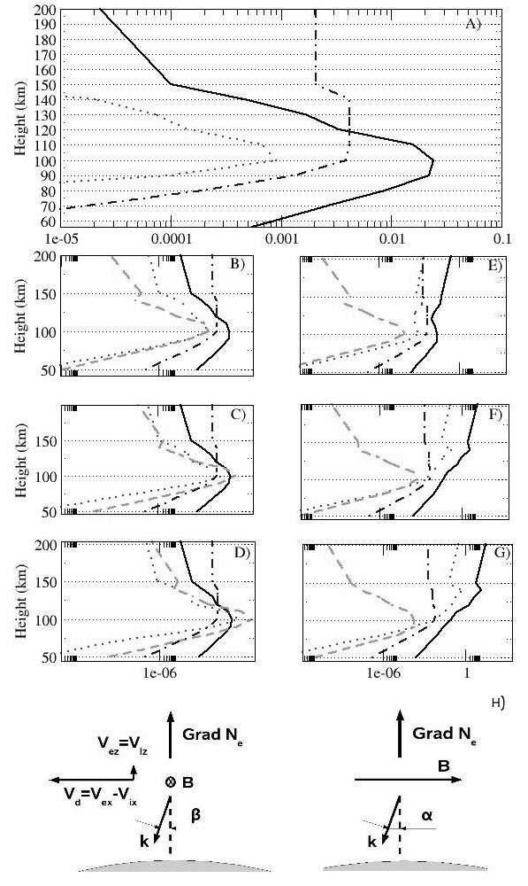
Figure 1: The absolute value of each term in the solution (9) in the equatorial ionosphere for different aspect ($\alpha$) and flow ($\beta$) angles. Figures (B-D) corresponds to different flow angles, correspondingly 1.0,10.0,30.0 degrees, for zero aspect angle. Figures (E-G) corresponds to the different aspect angles, correspondingly 0.1,1.0,3.0 degrees, for zero flow angle. Figure (A) corresponds to both angles are equal to zero. Terms: $\frac{\Psi}{1+\Psi}\frac{1}{\nu_{in}^{t,\mu}}C_{s}^{2}k^{2}$ - solid line; $\frac{\Psi}{1+\Psi}\frac{1}{\nu_{in}^{t,\mu}}\left(\frac{{\bf V_{0e}}+\Psi{\bf V_{0i}}}{1+\Psi}{\cdot}{\bf k}\right)^{2}$ - dotted line; $\frac{{\bf V}_{d}{\cdot}{\bf k}}{(1+\Psi)^{2}}\left(\frac{\nu_{in}^{t,\mu}}{\Omega_{i}}\right)\left\{\left(\frac{{\bf\bigtriangledown}N_{0}}{N_{0}k^{2}}\right){\cdot}\left({\bf b}\times{\bf k}\right)\right\}$ - dashed line; $\frac{{\bf V}_{e0}+{\bf V}_{i0}\Psi}{1+\Psi}{\cdot}\frac{{\bf\bigtriangledown}N_{0}}{N_{0}}$ - dot-dashed line. At Fig. (H) the geometry and explanation of $\alpha$ and $\beta$ is shown.

At Fig.1 we show a height dependence of the second, forth and fifth terms in (9) on the altitude for the described conditions. Geometry is shown at Fig.1(H). Figures 1B-D corresponds to different zenith angle in east-west plane (flow angle $\beta$, correspondingly 1.0,10.0,30.0 degrees, for zero aspect angle), figures E-G corresponds to the different zenith angle in north-south plane (aspect angle $\alpha$, correspondingly 0.1,1.0,3.0 degrees, for zero flow angle).

Figure 1A corresponds to both angles equal to zero. As one can see, at all heights the velocity divergence term $\frac{{\bf V}_{e0}+{\bf V}_{i0}\Psi}{1+\Psi}{\cdot}\frac{{\bf\bigtriangledown}N_{0}}{N_{0}}$ (dot-dashed line) in this case is much larger than standard F-B increment term $\frac{\Psi}{1+\Psi}\frac{1}{\nu_{in}^{t,\mu}}\left(\frac{{\bf V_{0e}}+\Psi{\bf V_{0i}}}{1+\Psi}{\cdot}{\bf k}\right)^{2}$ (dotted line) and due to this must be always taken into account. At heights above 115-120 km it becomes larger than decrement term $\frac{\Psi}{1+\Psi}\frac{1}{\nu_{in}^{t,\mu}}C_{s}^{2}k^{2}$ (solid line) and this fact can cause an additional growth of the instabilities. This term can be important, for example, for analysis of the echo at heights above 115km (see, for example, [Farely,2009, Fig.3]).

As one can also see, at flow angles higher than 10 degrees (Figure 1C-D) standard GD term $\frac{{\bf V}_{d}{\cdot}{\bf k}}{(1+\Psi)^{2}}\left(\frac{\nu_{in}^{t,\mu}}{\Omega_{i}}\right)\left\{\left(\frac{{\bf\bigtriangledown}N_{0}}{N_{0}k^{2}}\right){\cdot}\left({\bf b}\times{\bf k}\right)\right\}$ (dashed line) becomes important for generation of the instabilities, and it is well known fact (see, for example, [Farely,2009]). Also, as one can see, the effect of the new term will be stronger at larger wavelengths and weaker at smaller wavelengths.

It can be easily shown, that for lower part of ionospheric E-region, when electron density gradient and velocities are co-directed (this corresponds to the day conditions of the equatorial ionosphere), the last term increases the growth rate. In this case the possibility of observation of the irregularities becomes higher. When the electron density gradient and velocities are anti-directed (this corresponds to the night conditions of the lower part of E-layer of the equatorial ionosphere), the last term decreases the growth rate. In this case the possibility of observation of the irregularities becomes lower.

This effect - increasing of irregularities level at day and decreasing at night is observed at the 100-110 km. altitudes more-less regularly (see, for example, in [Farley,1985, Abdu et al.,2002, Denardini et al.,2005]). The similar hourly dependence of the irregularities is observed even at higher altitudes at equator (see, for example, in [Chau and Kudeki,2006]). It is important to note that daytime and nighttime power dynamics at 100-110km is explained for non-perpendicular wavevector and mean electron velocity by equatorial electrojet dynamics (see, for example, in [Farely,2009]), similar dynamics of scattered power at higher altitudes (above 130km) is still unexplained (see, for example, in [Chau and Kudeki,2006]). So the new term have similar dynamics and does not contradict with these known experimental results.

3.3 Quasi-polar case

Let us analyze the following case: strong geomagnetic disturbance produces almost horizontal ${\bf V_{0e}}={\bf V_{d}}=400m/s,{\bf V_{0i}}=0$, electron density gradient and magnetic field are nearly parallel (within 10 degrees) and almost vertical, wavevector nearly perpendicular to the magnetic field, $\frac{{\bf\bigtriangledown}N_{0}}{N_{0}}=10^{-4}m^{-1}$and vertical, wavevector $k=0.1m^{-1}$ and almost horizontal. In this case we can see that the last summand in the solution (8) is significant and the solution (8) becomes:

$$\omega_{r}+i\Gamma = \frac{{\bf V_{0e}}}{1+\Psi}{\cdot}{\bf k}+i\frac{\Psi}{1+\Psi}\frac{1}{\nu_{in}^{t,\mu}}\left(\left(\frac{{\bf V_{0e}}}{1+\Psi}{\cdot}{\bf k}\right)^{2}-C_{s}^{2}k^{2}\right)+$$ (10)

$$-i\left(2\alpha N_{0}\right)+i\frac{{\bf V}_{0e}{\cdot}{\bf k}}{(1+\Psi)^{2}}\left(\frac{\nu_{in}^{t,\mu}}{\Omega_{i}}\right)\left\{\left(\frac{{\bf\bigtriangledown}N_{0}}{N_{0}k^{2}}\right){\cdot}\left({\bf b}\times{\bf k}\right)\right\}+$$

$$+i\frac{{\bf V}_{0e}{\cdot}{\bf k}}{(1+\Psi)^{2}}\frac{m_{i}\nu_{in}^{t,\mu}}{m_{e}\nu_{en}^{t,\mu}k^{2}}\left(\left(\frac{{\bf\bigtriangledown}N_{0}}{N_{0}}{\cdot}{\bf b}\right)\left({\bf b}{\cdot}{\bf k}\right)\right)$$

As one can see, the last summand in expression (10) can produce instabilities at aspect angles larger than traditional theory predicts. The ”large aspect angles” effect is known in high latitude ionosphere and has different explanations (see, for example, in [Hamza and St.Maurice,1995] and references there). As also one can see, the new term do not depend on wavenumber, and standard F-B term increases with wavenumber growth. Due to this the presence of the last term will be more significant at larger wavelengths than at shorter ones.

At Fig.2 the numerical results are shown. Electron density gradient is supposed to be vertical, magnetic field does not have east-west component and is about 10 degrees off the zenith. Maximal drift velocity is 400m/s and oriented in north-south direction, which corresponds to average geomagnetic disturbance. Geometry is shown at Fig.2(H). Fig.2B-D shows dependence in the angle in plane perpendicular to the magnetic field (flow angle $\beta$, 1.0,3.0,10.0 degrees correspondingly, aspect angle 1.0 degree), Fig.2E-G shows dependence in plane of magnetic field line (aspect angle $\alpha$, 1.0,3.0,5.0 degrees correspondingly, zero flow angle). Fig 2A corresponds to the zero flow and aspect angles. As one can see, the new term (dot-dashed line) is not important at zero aspect angles, but becomes important at aspect angles 1-3 degrees (Fig.2E-F), and at these aspect angles can be responsible for generation of instabilities, when standard F-B increment term $\frac{\Psi}{1+\Psi}\frac{1}{\nu_{in}^{t,\mu}}\left(\frac{{\bf V_{0e}}+\Psi{\bf V_{0i}}}{1+\Psi}{\cdot}{\bf k}\right)^{2}$ (dotted line) is smaller than decrement term $\frac{\Psi}{1+\Psi}\frac{1}{\nu_{in}^{t,\mu}}C_{s}^{2}k^{2}$ (solid line). Due to specific orientation of the electron density gradient and magnetic field, the standard G-D term $\frac{{\bf V}_{d}{\cdot}{\bf k}}{(1+\Psi)^{2}}\left(\frac{\nu_{in}^{t,\mu}}{\Omega_{i}}\right)\left\{\left(\frac{{\bf\bigtriangledown}N_{0}}{N_{0}k^{2}}\right){\cdot}\left({\bf b}\times{\bf k}\right)\right\}$ (dashed line), is almost unimportant at these small flow angles.

As one can see, the new term can cause generation of the instabilities at larger aspect angles (Figs.2E-F).

4 Conclusion

Our analysis has shown that growth rate for gradient-drift instabilities has significant terms that depends on relative direction of electron density gradients, mean velocity and magnetic field directions (8). This leads to the different conditions for the growth of the F-B and G-D instabilities in the equatorial and auroral zones of the ionosphere. These terms are usually neglected [Fejer et al.,1975, Fejer et al.,1984, Farely,2009], but for building a general theory they must be taken into account.

At heights below 115km the full solution (8) transforms into standard one [Fejer et al.,1984], except the situations, when the electron density gradient is parallel to magnetic field or wave-vector. In these cases the new terms in the growth rate of the instabilities becomes significant and predicts the presence of gradient-drift instabilities even in these cases, as shown by expression (8), in opposite to traditional theory obtained in [Fejer et al.,1975, Fejer et al.,1984]. At low-latitude region these terms may cause additional growth of the instabilities at higher altitudes (above 115-120km). At high-latitude region these terms may produce changes of irregularities aspect sensitivity (large aspect angles effect). Both effects do not contradict with experimental data.

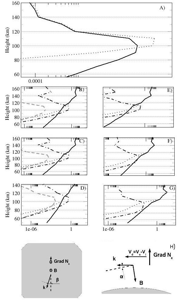
Figure 2: The absolute value of each term in the solution (10) in the high-latitude ionosphere for different aspect ($\alpha$) and flow ($\beta$) angles. Figures (B-D) corresponds to different flow angles , correspondingly 1.0,3.0,10.0 degrees, for 1.0 degree aspect angle. Figures (E-G) corresponds to the different aspect angles, correspondingly 1.0,3.0,5.0 degrees, for zero flow angle. Figure (A) corresponds to both 1.0 degree flow angle and zero aspect angle. Terms: $\frac{\Psi}{1+\Psi}\frac{1}{\nu_{in}^{t,\mu}}C_{s}^{2}k^{2}$ - solid line; $\frac{\Psi}{1+\Psi}\frac{1}{\nu_{in}^{t,\mu}}\left(\frac{{\bf V_{0e}}+\Psi{\bf V_{0i}}}{1+\Psi}{\cdot}{\bf k}\right)^{2}$ - dotted line; $\frac{{\bf V}_{d}{\cdot}{\bf k}}{(1+\Psi)^{2}}\left(\frac{\nu_{in}^{t,\mu}}{\Omega_{i}}\right)\left\{\left(\frac{{\bf\bigtriangledown}N_{0}}{N_{0}k^{2}}\right){\cdot}\left({\bf b}\times{\bf k}\right)\right\}$ - dashed line; $\frac{{\bf V}_{0e}{\cdot}{\bf k}}{(1+\Psi)^{2}}\frac{m_{i}\nu_{in}^{t,\mu}}{m_{e}\nu_{en}^{t,\mu}k^{2}}\left(\left(\frac{{\bf\bigtriangledown}N_{0}}{N_{0}}{\cdot}{\bf b}\right)\left({\bf b}{\cdot}{\bf k}\right)\right)$ - dot-dashed line. At Fig. (H) the geometry and explanation of $\alpha$ and $\beta$ is shown.

References

- [Abdu et al.,2002] M.A.Abdu, C.M.Denardini, J.H.A.Sobral, I.S.Batista, P.Muralikrishna, E.R. dePaula, //Journ. Atmosph. and Sol.-Terr.Phys. 64, 1425-1434, 2002
- [Akhiezer et al,1974] A.I. Akhiezer, I.A. Akhiezer, R.V. Polovin, A.G. Sitenko, and K.N. Stepanov. Plasma Electrodynamics, Volumes 1-2. Oxford: Pergamon Press, 1975
- [Buneman 1963] O.Buneman , Excitation of field aligned sound waves by electron streams// Phys.Rev.Lett. 10, 285-287, 1963
- [Chau and Kudeki,2006] J.L.Chau , E.Kudeki , Statistics of 150km echoes over Jicamarca based on low-power VHF observations //Ann.Geophys. 24, 1305-1310, 2006
- [Denardini et al.,2005] C.M.Denardini, M.A.Abdu, E.R. dePaula, J.H.A.Sobral, C.M.Wrasse, Seasonal characterization of the equatorial electrojet height rise over Brasil as observed by RESCO 50MHz back-scatter radar //Journ. Atmosph. and Sol.-Terr.Phys. 67, 1665-1673, 2005
- [Farley,1963] D.T.Farley, A plasma instability resulting in field-aligned irregularities in the ionosphere, //JGR 68, 6083-6097, 1963
- [Farley,1985] D.T.Farley, Theory of equatorial electrojet plasma waves: new developments and current system //JATP 47, 729-744, 1985
- [Farely,2009] D.T.Farley , The equatorial E-region and its plasma instabilities: a tutorial //Ann.Geophys. 27 1509-1520, 2009
- [Fejer et al.,1975] B.G.Fejer , D.T.Farley , B.B.Balsley and R.F.Woodman , Vertical Structure of the VHF Backscattering Region in Equatorial Electrojet and the Gradient Drift Instability, //JGR 80 1313-1324 , 1975
- [Fejer et al.,1984] B.G.Fejer, J.Providakes , D.T.Farley , Theory of plasma waves in the auroral E region, //JGR 89 7487-7494, 1984
- [Gelberg,1986] M.G.Gelberg, Irregularities of high-latitude ionosphere (In Russian), Novosibirsk, Nauka, 192pp., 1986
- [Golant et al.,1980] V.E.Golant , P.Zhilinsky and I.E.Sakharov, Fundamentals of Plasma Physics, 405pp., 1980
- [Gershman,1974] B.N.Gershman , Dynamics of the ionospheric plasma (In Russian), Moscow: Nauka, 256pp., 1974
- [Hamza and St.Maurice,1995] A.M.Hamza and J.-P. St.Maurice, Large aspect angles in auroral E-region echoes: a self-consistent turbulent fluid theory, //JGR 100 5723-5732, 1995
- [Rogister and D’Angelo,1970] Rogister,D’Angelo, Type II irregularities in the Equatorial electrojet //JGR 75, 3879-3887, 1970