Beating in electronic transport through quantum dot based devices

Abstract

Electronic transport through a two-level system driven by external electric field and coupled to (magnetic or non-magnetic) electron reservoirs is considered theoretically. The basic transport characteristics such as charge and spin current and tunnel magnetoresistance (TMR) are calculated in the weak coupling approximation by the use of rate equation connected with Green function formalism and slave-boson approach. The time dependent phenomenon is considered in the gradient expansion approximation. The results show that coherent beating pattern can be observed both in current and TMR. The proposed system consisting of two quantum dots attached to external leads, in which the dots’ levels can be tuned independently, can be realized experimentally to test this well known physical phenomenon. Finally, we also indicate possible practical applications of such device.

I Introduction

Beating is a well known phenomenon in physics.fishbane It occurs when the difference between frequencies of two interfering waves is small enough. As a result a long-wavelength pattern appears (with characteristic envelope changing very slowly). The resulting beating frequency is equal to one half of the difference in original wave frequencies. This effect is very important from both the fundamental and application points of view, as it provides a sensitive method for measuring the frequency difference. In music, for instance, the beating effect is used for tuning the instruments. This phenomenon is also utilized in conventional electronics to change the frequency of the input signal (in so called down conversion), which helps to improve sensitivity and selectivity of a receiver. Beating effect is also used in microwave spectroscopy.qin

Recently, it has turned out that beating phenomenon can be observed in different quantum systems like for instance, a single quantum dot (QD).gupta Discreteness of dot’s energy levels arising from quantum confinement make it able to mimic behavior of real atom, and is thus frequently referred to as artificial atom.reimann Moreover, beating has also been reported in a qubit coupled to a fluctuator being in contact with a heat bath.galperin ; loss The beating in Rabi oscillationssimmonds ; koppens were noticed, when the fluctuator is close to resonance with the qubit and the damping is weak enough.galperin Coherent beating in the magnetoresistance of ballistic tunnel junctions were also investigated.euges

The beating phenomenon in the occupation probability of excited state of a qubit has been predicted for Josephson qubit coupled resonantly to a two-level system (TLS), (i.e., the qubit and TLS have equal energy splittings).ku However, this was only true when there was any source of decoherence. This is also why the beating phenomenon has not yet been experimentally verified in such a system. In turn, control of electron spin coherence in quantum dots may be provided, for instance by circularly polarized laser pulses. Consequently, quantum dots may enable us to observe beating. In fact, the beating have already been noticed in a few experiments exploring time dependent Faraday rotationwieman ; gupta ; greilich in self-assembled QDs systems.

However, the beating phenomenon in electronic transport through laterally confined quantum dots systems is an unexplored field. Moreover, there is no experiment showing beating in transport characteristics of such nanoscale devices. So far, investigations were mainly focused on the spin-independent case, where only the coherent oscillations were reported.jauho93 ; jauho94 Recently, Souza has shown that the coherent oscillations become spin dependent when Zeeman splitting of the dot’s level and/or ferromagnetic leads are considered.souza In this case, the two spin components of the current oscillate with different frequencies and the beating is reported for relatively small splitting in the frequencies (i.e., dot’s level). Moreover, Prefetto et al. have shown that intradot spin-flip scattering suppresses the amplitude of the beating.stefanucci2 Recently, beating in current have been predicted due to the presence of Andreev bound states in dc biased QD system (coupled to superconducting leads) and irradiated with a microwave field of appropriate frequency.stefanucci3 More recently, the beating phenomenon in coherent transport through a microscale back-gated substrate coupled to optically gated quantum dot has been predicted when the Rabi frequencies approach the intrinsic Bohr frequencies in the dot.walczak

Here, we propose another quantum system, where the beating can be observed. Especially, we consider two single-level quantum dots attached to ferromagnetic/nonmagnetic leads or to spin batteries. Experimentally it can be fabricated making use of a two-dimensional electron gas formed at the interface of semiconductor heterostructure. The system is designed in specific way to avoid the channel mixing effects between the dots. Thus, the indirect coupling between the dots is eliminated. Moreover, the direct hopping is also excluded and the dots can be treated as independent. Charge, spin current and tunnel magnetoresistance (TMR) are derived in the weak coupling approximation utilizing rate equation associated with the Green function formalism as well as within the slave-boson approach.dong ; dong2 The gradient expansion is utilized to include time-dependent phenomenon.

The paper is organized as follows. In section II we describe the model and theoretical formalism. Numerical results on current and TMR are presented and discussed in section III. Summary and final conclusions are gathered in section IV.

II Model and theoretical formalism

We consider two single-level quantum dots coupled to external electrodes (magnetic or nonmagnetic). Moreover, nonmagnetic leads can be driven by both charge and spin bias voltage. The quantum dots are attached to the leads as shown in Fig.1. As channel mixing effectstrocha are minimized, we are allowed to introduce two independent transport channels, provided some additional assumptions are also made. Specifically, we also eliminate direct hopping between the dots (by creation of sufficiently wide and high tunnel barrier between them). The indirect coupling may be significantly reduced in comparison to dot-lead coupling when, for instance destructive interference effects take place. In real systems such processes are present leading to suppression of the channel mixing effects. As the interdot Coulomb interactions are at least an order of magnitude smaller than the intradot Coulomb interactions, we omit the former.

Then Hamiltonian of the system is as follows:

$$\hat{H} =\sum_{\mathbf{k}\alpha\sigma}\varepsilon_{{\mathbf{k}}\alpha\sigma}c^{\dagger}_{{\mathbf{k}}\alpha\sigma}c_{{\mathbf{k}}\alpha\sigma}+\sum_{i=1,2}\sum_{\sigma}\limits\epsilon_{i\sigma}(t)q^{\dagger}_{i\sigma}q_{i\sigma}$$

$$+\sum_{i=1,2}\limits U_{i}n_{i\sigma}n_{i\bar{\sigma}}+\sum_{{\mathbf{k}}\alpha}\sum_{i,\sigma}\limits(V_{i\sigma}^{\alpha}c^{\dagger}_{{\mathbf{k}}\alpha\sigma}q_{i\sigma}+\rm H.c.).\ \$$ (1)

The first term describes here the three leads in the non-interacting quasi-particle approximation, where $\alpha=S1,S2,D$ means two sources and one drain leads. Here, $c^{\dagger}_{\mathbf{k}\alpha\sigma}$ ($c_{\mathbf{k}\alpha\sigma}$) is the creation (annihilation) operator of an electron with the wave vector $\mathbf{k}$ and spin $\sigma$ in the lead $\alpha$, whereas $\varepsilon_{\mathbf{k}\alpha\sigma}$ denotes the corresponding single-particle energy. The next two terms in the Hamiltonian (II) describe the two quantum dots. Here, $n_{i\sigma}=q^{\dagger}_{i\sigma}q_{i\sigma}$ is the particle number operator ($i=1,2$, $\sigma=\uparrow,\downarrow$), $\epsilon_{i\sigma}(t)$ is the discrete energy level of the $i$-th dot (including time dependence of the corresponding gate voltage), and $U_{i}$ is the intra-dot Coulomb integral. The last term of Hamiltonian (II) describes electron tunneling between the leads and dots, where $V_{i\sigma}^{\alpha}$ are the relevant tunneling matrix elements. Coupling of the dots to external leads can be parameterized in terms of $\Gamma^{\alpha}_{i\sigma}(\epsilon)=2\pi\sum_{\mathbf{k}}V_{i\sigma}^{\alpha}V^{\alpha\ast}_{i\sigma}\delta(\epsilon-\varepsilon_{\mathbf{k}\alpha i})$. We assume that $\Gamma^{\alpha}_{i\sigma}$ is constant within the electron band, $\Gamma^{\alpha}_{i\sigma}(\epsilon)=\Gamma^{\alpha}_{i\sigma}={\rm const}$ for $\epsilon\in\langle-W/2,W/2\rangle$, and $\Gamma^{\alpha}_{i\sigma}(\epsilon)=0$ otherwise. Here, $W$ denotes the electron band width.

As in our model the dots are independent – they do not interact with each other – one can decompose the density matrix operator of the whole system as follows $\hat{\rho}_{total}=\hat{\rho}_{1}\otimes\hat{\rho}_{2}$ and consider each subsystem (each dot coupled to the source and drain leads) separately.

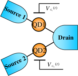
Figure 1: Schematic picture of two dots coupled to external leads. Each dot is attached to its own source lead, whereas the drain electrode is the same for the two dots.

Furthermore, we adopt the formalism presented in Ref.[dong, ]. Specifically, we express i-th dot’s operator in terms of Hubbard operatorshubbard represented by four possible electron states in each dotanderson which satisfied the corresponding completeness relations.dong In the next step, the set of auxiliary operators is introduced and the dots’ operators are expressed by means of these slave-boson and pseudofermion operators. From the definitions of the Dirac brackets one is able to find the commutations (and anticommutations) rules for new operators.guillou Therefore, the Hamiltonian of the system acquires the form:

$$\hat{H} =\sum_{\mathbf{k}\alpha\sigma}\varepsilon_{{\mathbf{k}}\alpha\sigma}c^{\dagger}_{{\mathbf{k}}\alpha\sigma}c_{{\mathbf{k}}\alpha\sigma}+\sum_{i\sigma}\limits\epsilon_{i\sigma}(t)(f^{\dagger}_{i\sigma}f_{i\sigma}+d_{i}^{{\dagger}}d_{i})$$

$$+\sum_{i}\limits U_{i}d_{i}^{{\dagger}}d_{i}+\sum_{{\mathbf{k}}\alpha}\sum_{i\sigma}\limits[V_{i\sigma}^{\alpha}c^{\dagger}_{{\mathbf{k}}\alpha\sigma}(e_{i}^{{\dagger}}f_{i\sigma}+\sigma f_{i\bar{\sigma}}^{{\dagger}}d_{i})+\rm H.c.].$$ (2)

Here, $b_{i}^{{\dagger}}$ is the slave-boson operator which creates an empty state in $i$th dot, $f^{{\dagger}}_{i\sigma}$ is a peudo-fermion operator which creates a singly occupied state with an electron with spin $\sigma$, whereas $d_{i}^{{\dagger}}$ creates doubly occupied state with an electron with spin $\sigma$ and other electron with spin $\bar{\sigma}$ in $i$th dot.

In the slave-particle representation the density matrix elements (for each subsystem) are written in the following way: $\hat{\rho}_{00}^{i}=e_{i}^{{\dagger}}e_{i}$, $\hat{\rho}_{\sigma\sigma}^{i}=f_{i\sigma}^{{\dagger}}f_{i\sigma}$, $\hat{\rho}_{22}^{i}=d_{i}^{{\dagger}}d_{i}$. Here, the statistical expectations of the density matrix elements ($\rho_{nn}^{i}\equiv\langle\hat{\rho}_{nn}^{i}\rangle$ with $n=0,\sigma,2$) give the occupation probabilities of the given quantum dot being empty, singly occupied by electron with spin-$\sigma$, or doubly occupied, respectively.

To derive the rate equations we start from the von Neumann equation for density matrix operator:

$$\dot{\hat{\rho}}_{j}=i[H,\hat{\rho}_{j}],$$ (3)

where $\hat{\rho}_{j}=(\hat{\rho}_{00}^{j},\hat{\rho}_{\uparrow\uparrow}^{j},\hat{\rho}_{\downarrow\downarrow}^{j},\hat{\rho}_{22}^{j})^{T}$ with $j=1,2$. The obtained averaged equations for density matrix elements can be expressed by means of dot-lead Green functions. Furthermore, using Langreth theoremjauho93 , we express the dot-lead Green functions by means of dot’s Green functions and free leads’ Green functions. After utilizing gradient expansion approximation these Green functions can be written in the $\omega$ space in the following way:

$$G^{<}_{k\alpha\sigma,e\sigma}(\omega,\bar{t}) =V_{\alpha\sigma}[g_{k\alpha\sigma}^{r}G_{e\sigma\sigma}^{<}(\omega,\bar{t})+g_{k\alpha\sigma}^{<}G_{e\sigma\sigma}^{a}(\omega,\bar{t})],$$

$$G^{<}_{e\sigma,k\alpha\sigma}(\omega,\bar{t}) =V_{\alpha\sigma}^{\ast}[G_{e\sigma\sigma}^{r}(\omega,\bar{t})g_{k\alpha\sigma}^{<}+G_{e\sigma\sigma}^{<}(\omega,\bar{t})g_{k\alpha\sigma}^{a}],$$

$$G^{<}_{k\alpha\sigma,d{\bar{\sigma}}}(\omega,\bar{t}) =V_{\alpha\sigma}[g_{k\alpha\sigma}^{r}G_{d\bar{\sigma}\bar{\sigma}}^{<}(\omega,\bar{t})+g_{k\alpha\sigma}^{<}G_{d\bar{\sigma}\bar{\sigma}}^{a}(\omega,\bar{t})],$$

$$G^{<}_{d\sigma,k\alpha\sigma}(\omega,\bar{t}) =V_{\alpha\sigma}^{\ast}[G_{d\bar{\sigma}\bar{\sigma}}^{r}(\omega,\bar{t})g_{k\alpha\sigma}^{<}+G_{d\bar{\sigma}\bar{\sigma}}^{<}(\omega,\bar{t})g_{k\alpha\sigma}^{a}],$$ (4)

where the free leads lesser ($<$), retarded ($r$) and advanced ($a$) Green functions have the following form:

$$g_{k\alpha\sigma}^{<}= i2\pi f^{\alpha}(\omega)\delta(\omega-\varepsilon_{{\mathbf{k}}\alpha\sigma})$$ (5)

$$g_{k\alpha\sigma}^{r,a}= P\left(\frac{1}{{\omega}-\varepsilon_{{\mathbf{k}}\alpha\sigma}}\right)\mp i\pi\delta(\omega-\varepsilon_{{\mathbf{k}}\alpha\sigma}),$$ (6)

with $f^{\alpha}(\omega)$ being Fermi-Dirac function for the $\alpha$ lead. In the above equation and in further considerations we omit the dot’s index $i$ as the further equations for both QD’s acquire the same form. In Eq.(II) the Green functions of the dot, in time space, are defined as: $G_{\sigma\sigma}(t,t^{\prime})=\langle\langle q_{\sigma}(t)|q_{\sigma}^{{\dagger}}(t^{\prime})\rangle\rangle=\langle\langle e_{\sigma}^{{\dagger}}(t)f_{\sigma}(t)|f_{\sigma}^{{\dagger}}(t^{\prime})e(t^{\prime})\rangle\rangle+|\sigma|^{2}\langle\langle f_{\bar{\sigma}}^{{\dagger}}(t)d(t)|d^{{\dagger}}(t^{\prime})f_{\bar{\sigma}}(t^{\prime})\rangle\rangle$. Other parts of $G_{\sigma\sigma}(t,t^{\prime})$ vanish for $t^{\prime}=t$, thus are omitted as we are interested in $t^{\prime}=t$ case. Furthermore, for the sake of simplicity we will omit the real part in $g_{k\alpha\sigma}^{r,a}$ which is justified in wide band limit. Combining earlier obtained rate equations with Eq.(II) we arrive with the rate equations expressed in Fourier space in the following form:

$$\dot{\rho}_{00}= -\frac{i}{2\pi}\int d\omega\sum_{\alpha\sigma}[\Gamma_{\sigma}^{\alpha}f^{\alpha}(\omega)G^{>}_{e\sigma\sigma}(\omega,\bar{t})$$

$$+\Gamma_{\sigma}^{\alpha}(1-f^{\alpha}(\omega))G^{<}_{e\sigma\sigma}(\omega,\bar{t})]$$

$$\dot{\rho}_{\sigma\sigma}= \frac{i}{2\pi}\int d\omega\sum_{\alpha}[\Gamma_{\sigma}^{\alpha}f^{\alpha}(\omega)G^{>}_{e\sigma\sigma}(\omega,\bar{t})$$

$$+\Gamma_{\sigma}^{\alpha}(1-f^{\alpha}(\omega))G^{<}_{e\sigma\sigma}(\omega,\bar{t})-\Gamma_{\bar{\sigma}}^{\alpha}f^{\alpha}(\omega)G^{>}_{d\sigma\sigma}(\omega,\bar{t})$$

$$-\Gamma_{\bar{\sigma}}^{\alpha}(1-f^{\alpha}(\omega))G^{<}_{d\sigma\sigma}(\omega,\bar{t})]$$

$$\dot{\rho}_{22}= \frac{i}{2\pi}\int d\omega\sum_{\alpha\sigma}[\Gamma_{\sigma}^{\alpha}f^{\alpha}(\omega)G^{>}_{d\bar{\sigma}\bar{\sigma}}(\omega,\bar{t})$$

$$+\Gamma_{\sigma}^{\alpha}(1-f^{\alpha}(\omega))G^{<}_{d\bar{\sigma}\bar{\sigma}}(\omega,\bar{t})]$$ (7)

As the transition from time space to the Fourier space in the time dependent phenomena is not straightforward it is required to justified it. Therefore, we introduced new time variables: a mean time $\bar{t}=\frac{t+t^{\prime}}{2}$ which varies slowly and a fast varying time difference $\delta t=t-t^{\prime}$, and expressed the Green functions in these new time scales, i.e. $G(t,t^{\prime})\longrightarrow G(\delta t,\bar{t})$.davis ; hernandez Expanding $G(\delta t,\bar{t})$ in the slow variable ($\bar{t}$) and taking the Fourier transform with respect to the fast variable, we arrive at the Green function $G(\omega,\bar{t})=\sum_{n}\bar{G}^{(n)}(\omega,\bar{t})\bar{t}^{n}$ with $\bar{G}^{(n)}$ being n-th derivative (of the $G(\omega,\bar{t})$) with respect to the slow variable. Then, we retain only the first term in this expansion which allows us to write the lesser dot-leads Green function as in Eq.(II) This (lowest order) gradient expansion is sufficient approach as we are interested in sequential tunneling regime.davis After exploiting the above obtained equations, the rate equations acquire form as these presented in Ref.[dong, ] when putting intradot spin-flip parameter $R_{\sigma}$ to be equal to zero. However, in the situation considered here, the dots’ Green functions depends on both $\omega$ and the mean time $\bar{t}$. The dots’ Green functions we find in the weak coupling approximation, deriving them from corresponding equation of motion for the dots operators. Technically, we assumed there is no coupling ($V_{i\sigma}^{\alpha}=0$) and that leads are taken to be in local thermal equilibrium. Thus, we obtained:

$$G^{<}_{e\sigma\sigma}(\omega,\bar{t}) =i2\pi\rho_{\sigma\sigma}\delta(\omega-\epsilon_{\sigma}(\bar{t}))$$

$$G^{>}_{e\sigma\sigma}(\omega,\bar{t}) =-i2\pi\rho_{00}\delta(\omega-\epsilon_{\sigma}(\bar{t}))$$

$$G^{<}_{d\bar{\sigma}\bar{\sigma}}(\omega,\bar{t}) =i2\pi\rho_{22}\delta[\omega-(\epsilon_{\sigma}(\bar{t})+U)]$$

$$G^{>}_{d\bar{\sigma}\bar{\sigma}}(\omega,\bar{t}) =-i2\pi\rho_{\bar{\sigma}\bar{\sigma}}\delta[\omega-(\epsilon_{\sigma}(\bar{t})+U)],$$ (8)

where the time dependence is clearly emphasized. To derive these Green functions we used adiabatic approximation expanding $\epsilon_{\sigma}(t)$ around the mean time $\bar{t}$ and kept the terms up to linear order in the slow variable, namely $\epsilon_{\sigma}(\tau)\approx\epsilon_{\sigma}(\bar{t})+\dot{\epsilon}_{\sigma}(\tau)|_{\tau=\bar{t}}(\tau-\bar{t})$. This allowed us to write $\int_{t^{\prime}}^{t}dt_{1}\epsilon_{\sigma}(\tau)\approx\epsilon_{\sigma}(\bar{t})\delta t$. Then, after making Fourier transformation, Eqs. (II) are obtained. Finally, connecting Eqs.(II) with Eqs.(II) we arrive at the coupled set of differential equations which we solve numerically to obtain time dependence of the density matrix elements.

Current flowing from $\alpha$ ($\alpha=S1,S2,D$) lead to the $j$th dot is obtained from the standard definition:

$$J_{\alpha}^{j}=-e\langle\dot{N}_{\alpha}\rangle=-i\frac{e}{\hbar}\langle[H,N_{\alpha}]\rangle,$$ (9)

where $N_{\alpha}$ is an occupation number operator in $\alpha$ lead. After performing similar calculation as above, the current formula becomesdong :

$$J_{\alpha}^{j} =i\frac{e}{\hbar}\int\frac{d\omega}{2\pi}\sum_{\sigma}\limits\Gamma_{j\sigma}^{\alpha}f^{\alpha}(\omega)[G^{>}_{e\sigma\sigma}(\omega,\bar{t})+G^{>}_{d\bar{\sigma}\bar{\sigma}}(\omega,\bar{t})]$$

$$+\Gamma_{j\sigma}^{\alpha}[1-f^{\alpha}(\omega)][G^{<}_{e\sigma\sigma}(\omega,\bar{t})+G^{<}_{d\bar{\sigma}\bar{\sigma}}(\omega,\bar{t})].$$ (10)

Current passing through $j$th dot can be symmetrized in the following way: $J^{j}=(J^{Sj}_{j}-J^{D}_{j})/2$. Total current flowing through the system is equal to $J=J^{1}+J^{2}$. We assume that the distance between contacts in the drain lead is lesser than coherence length.

III Numerical Results

Time-dependent phenomenon is investigated in electronic transport through two quantum dots coupled to external leads as shown schematically in Fig.1. The dots’ levels are driven by time-dependent gate voltages (ac force), whereas the dot-lead couplings are assumed to be constant in time. Each dot has its own gate electrode, thus the dots’ levels can be tuned independently. Moreover, this allows to apply AC voltages to two dots with distinct external frequency and driving amplitudes. It is worth nothing that this can not be achieved in multilevel single quantum dot.

We consider the dots’ levels driven by sinusoidal AC voltage, and thus we assume $\epsilon_{i\sigma}(t)=\epsilon_{i\sigma}+\delta_{i}\cos{\Omega_{i}t}$. Here, $\Omega_{i}$ is frequency, whereas $\delta_{i}$ is amplitude of the external signal applied to the $i$th dot. In our model, the chemical potentials of the source and drain leads are set as $\mu_{S1}=\mu_{S2}=eV/2$ and $\mu_{D}=-eV/2$. Here, $V$ is a bias voltage applied between the source (S1, S2) and drain leads. Before the time dependent signals drive the dots’ levels, the system is in deep nonequilibrium due to applied bias voltage. Thus, one should expect the dynamics of the system undergoes non-Marcovian processes. In numerical calculations we assume that each dot is equally coupled to its pair of leads, namely, $\Gamma_{1}^{S}=\Gamma_{2}^{S}=\Gamma_{1}^{D}=\Gamma_{2}^{D}=\Gamma$ with $\Gamma$ being the energy unit. Moreover, we assume spin degenerate and equal time-independent parts of the dot levels, $\epsilon_{i\sigma}=\epsilon_{0}$ (for $i=1,2$ and $\sigma=\uparrow,\downarrow$) and equal amplitudes of the oscillating signals ($\delta_{1}=\delta_{2}=\delta$). For simplicity we also assume the same Coulomb parameters for the two dots, $U_{1}=U_{2}=U$.

Approximations made during calculation of the rate equations and current formula (gradient expansion and weak coupling) constrict our model to special regimes. There are two regimes when this approximation is valid: i) when $\epsilon_{i}\approx\mu_{Si}$ then must be $\hbar\Omega\ll k_{B}T$, $\Gamma\ll k_{B}T$, ii) when $-W/2<\epsilon_{i}<\mu_{Si}$ is valid for $\hbar\Omega\ll W$ and $\Gamma\ll W$.davis In our numerical calculations we choose a set of parameters which fulfill these limitations. Moreover, we assume that the system initially occupies the empty state $\rho^{(1,2)}_{00}=1$. In our calculations we also set $h\equiv 1$.

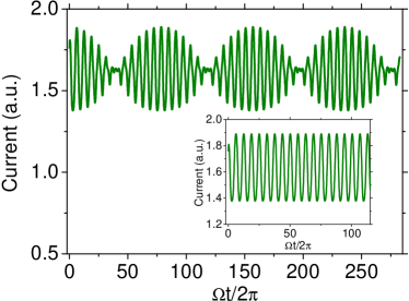
Figure 2: Current as a function of time calculated for nonmagnetic leads and for different driving frequencies $\Omega_{1}=1.04\Omega$, $\Omega_{2}=0.96\Omega$. The inset shows current evolution calculated for nonmagnetic leads and for equal driving frequencies $\Omega_{1}=\Omega_{2}=\Omega$. Other parameters: $\epsilon_{0}=-\Gamma$, $\delta=0.2\Gamma$, $U=\Gamma$, $k_{B}T=0.1\Gamma$, $eV=2\Gamma$. Here, $\Omega$ is chosen to be frequency unit.

III.1 Nonmagnetic leads

At the beginning we consider quantum dots coupled to nonmagnetic leads and assume that dots’ levels are driven by gate voltages with different frequencies ($\Omega_{1}\neq\Omega_{2}$) but equal amplitudes ($\delta_{1}=\delta_{2}$). When the external frequencies differ only a little, the beating in current are observed as shown in Fig.2. Total current beats with frequency being twice the difference of the frequencies of the currents passing through each quantum dot. Thus, the total current can be decomposed as a product of two parts: one oscillates with the average frequency $F=\frac{1}{2}(f_{1}+f_{2})$ and second changing with the frequency $\Delta f=\frac{1}{2}(f_{1}-f_{2})$, where $f_{1}=\Omega_{1}/2\pi$ and $f_{2}=\Omega_{2}/2\pi$ are corresponding frequencies of the currents flowing through each dot. The latter term controls the amplitude of the envelope and is responsible for the sensing of beating. The beating frequency is twice the difference frequency $F_{b}=2\Delta f$. Thus, the beating frequency is lowered when reducing the difference in the frequencies of the input signals. This effect is only due to the difference in the frequencies of the external gate voltages. To show this we calculated the current evolution for equal external frequencies $\Omega_{1}=\Omega_{2}$ and displayed it in inset of Fig.2. Thus, we believe that this system is favorable for observing current’s beating in experiment. In contrast to results presented in Ref.[souza, ], where the beating signal is damped (due to the dot-lead coupling), in our case beating of the current is sustained in time.

In Fig.3 we show the influence of the temperature on the current’s beating. We notice that the amplitude of the beating signal is damped as temperature increases. However, even for $k_{B}T\gg\Gamma$ the beating pattern can still exist what is clearly shown in the zoomed part of Fig.3. In turn, the amplitude of the beating can be increased by enlarging the amplitudes of the input signals ($\delta$). This implies that even for $k_{B}T>\Gamma$ the current’s beating survives and may be observed when $\delta$ is sufficiently large. We also noticed that average current drops with increasing temperature, which is due to thermal damping effect in the leads.

Our calculations have also shown that intradot Coulomb interactions do not destroy beating pattern in current. To show this we plot in Fig.4 beating current for different values of the Hubbard parameter $U$. However, the Coulomb repulsion influences both the amplitude of the beating and the value of the average current. Namely, when there is no Coulomb interaction, the amplitude of the beating is most pronounced. When the on-dot Coulomb repulsion is present, the amplitude of the beating is suppressed. The dependence of the beating’s amplitude is nonmonotonic function of the parameter $U$. When $\epsilon_{0}+U$ is within the transport window it decays with increasing $U$, but for $\epsilon_{0}+U>\mu_{S}$ it starts to increase. However, it never again reaches the maximum value.

The average current is a also nonmonotonic function of the Coulomb parameter $U$. It reaches high values when $\epsilon_{0}\approx\mu_{D}$ and $\epsilon_{0}+U$ approaches $\mu_{Sj}$ (but not very close, $\epsilon_{0}+U\ncong\mu_{Sj}$, due to imposed gradient’s expansion condition.) When $\epsilon_{0}+U$ is beyond the transport window, average current drops and saturates for sufficiently large $U$. Moreover, Coulomb interactions introduce small horizontal asymmetry in the beating pattern.

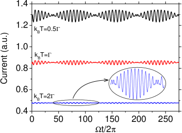
Figure 3: Beating current calculated for indicated values of the temperature. Other parameters as in Fig.2. In the ellipse we show zoomed part of the plot encircled in the frame.

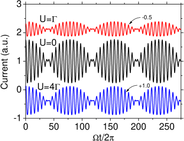
Figure 4: Beating current calculated for indicated values of the intradot Coulomb repulsion parameter. Other parameters as in Fig.2. Here, for clarity we rescaled the current plot for $U=\Gamma$ and $U=4\Gamma$. To obtain calculated values of the current for those parameter one has to add certain value to all points as is indicated by arrows.

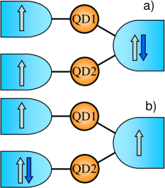
Figure 5: Magnetic configurations taken into account.

III.2 Ferromagnetic leads

When, the leads are ferromagnetic several magnetic configurations are possible. To ’measure’ the difference in these distinct configurations it is convenient to introduce tunnel magnetoresistance (TMR). This quantity results from spin-dependent dot-lead tunneling processes, which in turn leads to the dependence of transport characteristics on magnetic configuration of the system. The TMR is quantitatively described by the ratio ${\rm TMR}=I_{P}-I_{AP}/I_{AP}$, where $I_{P}$ and $I_{AP}$ denote the currents flowing through the system in the parallel and antiparallel magnetic configurations, respectively.

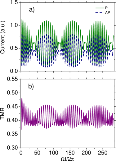
Figure 6: a) Current as a function of time calculated for two magnetic configurations from Fig.5(a) and for $p=0.5$, $U=4\Gamma$. b) Time evolution of TMR. Other parameters as in Fig.2.

Introducing the spin polarization $p_{\alpha}$ of lead $\alpha$ ($\alpha=S1,S2,D$) as $p_{\alpha}=(\rho_{\alpha}^{+}-\rho_{\alpha}^{-})/(\rho_{\alpha}^{+}+\rho_{\alpha}^{-})$, the coupling parameters can be expressed as $\Gamma_{i\alpha}^{+(-)}=\Gamma_{i\alpha}(1\pm p_{\alpha})$, with $\Gamma_{i\alpha}=(\Gamma_{i\alpha}^{+}+\Gamma_{i\alpha}^{-})/2$. Here, $\rho_{\alpha}^{+}$ and $\rho_{\alpha}^{-}$ are the densities of states at the Fermi level for spin-majority and spin-minority electrons in the lead $\alpha$, while $\Gamma_{i\alpha}^{+}$ and $\Gamma_{i\alpha}^{-}$ describe coupling of the $i$th dot to the lead $\alpha$ in the spin-majority and spin-minority channels, respectively.

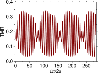
Figure 7: Time dependence of the TMR calculated for magnetic configurations from Fig.5(b). Other parameters as in Fig.6.

Let us first consider the case where the magnetic moments of the source leads are pinned (with ’up’ direction) and the magnetization of the drain electrode can be changed from ’up’ to ’down’ as schematically is shown in Fig.5(a). We calculated the currents in both magnetic configurations and TMR for leads’ polarization $p_{S1}=p_{S2}=p_{D}=0.5$. Firstly, one observes that the beating is still present in the current characteristics for both magnetic configurations. However, TMR exhibits beating pattern a little distorted. As the dots are decoupled from each other and we consider the case of weak couplings we should expect positive TMR, which is clearly displayed in Fig.6(b). Then, off course, the current in parallel magnetic configuration is greater than that in antiparallel one (see Fig.6(a)). However, spin symmetry breaking processes, as spin-flip scattering, may change the sign of TMR as shown in Ref.[stefanucci2, ]. Here, we do not consider such processes. Recent experiments have shown that the spin relaxation time in quantum dots can reach millisecondelzerman ; johnson ; koppens or even second timescalesamasha which is much longer than electron tunnel rate ($\sim\Gamma^{-1}$).

Now, we consider the situation when the magnetization of the drain lead and one of the source electrode are pinned, whereas the magnetic moment of the second source lead can be flipped, as is shown in Fig.5(b). In this case, the difference between ’parallel’ and ’antiparallel’ configurations is less visible, which results in suppression of TMR. However, the oscillating character is still conserved and here the beating is even more pronounced (see Fig.7). The suppression of the TMR for this magnetic configurations is clear when one notices that for this case only one transport channel is partially blocked (due to relevant difference in the orientations of the leads magnetic moments in the AP configuration), whereas in the former case both channels are bad ’conductors’ in the AP configuration. Moreover, in this magnetic configuration, $\pi/2$ phase shift is induced in the TMR pattern. A small distortion in the upper semicircles comes from the different symmetries of the current profiles for P and AP configurations in the vicinity of the node points.

III.3 Spin-biased leads

Here, we consider the double dots’ system subjected to the source and drain spin batterieshirsch ; brouver ; wang2 which provides pure spin current without accompanying charge current. Pure spin current is one of the most important points for spintronics. However, so far spin control methods in commercial devices mainly have relied on usage of magnetic fieldmucciolo ; watson or optical techniques which are not very efficient. Recent experiments show that pure spin current can be all-electrically generated in a micron-wide channels of a GaAs two-dimensional electron gasfrolov1 ; frolov2 . This is very important from the application point of view, because other quantum systems can be easily integrated with such all-electrically controllable spin battery. To control such a device we do not need optical or magnetic fields which precisely adjusting is rather great effort and thus, useless for commercial applications.

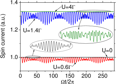
Figure 8: Time evolution of the spin current calculated for indicated values of the intradot Coulomb repulsion parameter and for $\epsilon_{0}=0$ in case of the symmetric spin batteries. Other parameters as in Fig.2.

First, we investigate DQD system connected to symmetric dipolar spin batteries, i.e. we assume that $\mu_{Sj\uparrow}=\mu_{D\downarrow}$ and $\mu_{Sj\downarrow}=\mu_{D\uparrow}$ for ($j=1,2$). Introducing the spin bias $V_{s}$, generally we may write $\mu_{Sj\sigma}=e(V+\tilde{\sigma}V_{s})/2$ and $\mu_{D\sigma}=-e(V+\tilde{\sigma}V_{s})/2$ with $\tilde{\sigma}=1$ ($\tilde{\sigma}=-1$) for $\sigma=\uparrow$ ($\sigma=\downarrow$)swirkowicz . As we are interested in pure spin current we further set bias voltage equal to zero $V=0$. In this case the net charge current vanishes, because all spin-up electrons flow in one direction and equal amount of spin-down electrons flow in the opposite direction, and only pure spin current is generated. The spin current is defined in the following way, $J_{s}=(J_{\uparrow}-J_{\downarrow})/e$, where $J_{\sigma}=J_{\sigma}^{1}+J_{\sigma}^{2}$ ($\sigma=\uparrow,\downarrow$). However, it is worth to mention that when the dot’s energy level is split i.e., $\epsilon_{\uparrow}\neq\epsilon_{\downarrow}$, the nonzero charge current can be generatedwang2 ; bao ; swirkowicz . In Fig.8 we show time evolution of the spin current calculated for different strengths of the intradot Coulomb interactions. One can notice that the spin current exhibits more complicated beating pattern (similar as TMR in Fig.6). On the other hand, for noninteracting case ($U=0$) we notice the clear evidence of pure beats in the spin current. However, for this case the amplitude of the beating is small. When Coulomb interactions are turned on, symmetric beating pattern vanishes and even more features appear. As intradot repulsion increases, the beating in the spin current become more and more asymmetric and the node points cease to exist. Instead of node new oscillations emerge. Namely, for nonzero $U$, spin current evolution composes from two kind of oscillations: main oscillations and some sub-oscillations emerged in the vicinity of the nodes points (existing in noninteracting case). For sufficiently large $U$, the main oscillations become very asymmetric and the sub-oscillations are more pronounced. In contrast to the nonmagnetic case, the dependence on the Coulomb repulsion is here much more complex. The amplitude of the beating is small for both small and large enough $U$. This is because the state $\epsilon_{0}+U$ is far away from the chemical potentials of the leads. However, when $\epsilon_{0}+U$ is outside the transport window, the average spin current grows meaningly (in contrast to the charge current in nonmagnetic case from Fig.4). When $U$ is sufficiently large (i.e. $\epsilon_{0}+U\gg\mu_{\alpha\sigma}$) the probability of double occupancy drops almost to zero ($\rho_{22}\approx 0$) and the occupation numbers $n_{\sigma}$ also decrease (however $\rho_{\sigma}$ increases). This enables effectively faster tunelling processes through QD and thus enlarges the spin current. For $U\gg\mu_{\alpha\sigma}$ the spin current becomes saturated.

Figure 9: Stationary charge (a) and spin (b) current as a function of the Coulomb repulsion parameter $U$. Insets: Time evolution of the charge and spin current,respectively, calculated for for $\epsilon_{0}=0$ and for $U=0$, in case of the asymmetric spin batteries. Other parameters as in Fig.2.

Now, we consider DQD system attached to asymmetric spin batteries. In this case we set $\mu_{Sj\sigma}=\tilde{\sigma}eV_{s}$ and $\mu_{D\sigma}=0$. Let us first consider noninteracting case ($U=0$). The dots’ energy levels are situated symmetrically with respect to the spin bias voltages of the source leads, e.g., $\epsilon_{0}$ is in the mid between $\mu_{Sj\uparrow}$ and $\mu_{Sj\downarrow}$. Thus, the same amount of spin-up electrons flows in one direction and equal amount of spin-down electrons flows in the opposite direction and the average spin current is nonzero. However, due to oscillations of the dots’ levels, the charge current is also generated, but on average it vanishes. In the case of asymmetric spin batteries both the spin and charge current exhibits well-defined beating pattern as shown in the insets of Fig.9. When the Coulomb interactions are turned on, a nonzero average charge current is induced. This is because earlier mentioned symmetry is now broken. It is worth noting that such symmetry exists also when $\epsilon_{0}=-U/2$. However, for $\epsilon_{0}<\mu_{D}$ and sufficiently large $U$ the system is in the Coulomb blockade, thus, we expect zero current in the weak coupling regime. Firstly, for a small value of the parameter $U$, the average charge current grows very fast reaching maximum value for $U\approx 0.4\Gamma$ and then is unchanged with further increase of the $U$, until $\epsilon_{0}+U$ exceeds $\mu_{Sj\uparrow}$, when it becomes reduced a little and saturates. This drop in average charge current is because the state $\epsilon_{0}+U$ ceases to contribute to the transport. In turn, the average spin current, generally, grows with increasing parameter $U$ (regardless a certain ranges of $U$ where the average spin current is constant). When $U$ is sufficiently large the average spin current is also saturated. To show this dependencies we plotted stationary charge and spin current in Fig.9 which may be regarded as average values of respective currents in time-dependent phenomenon. However, one should bear in mind that this is not true for $\epsilon_{0}+U$ being close to $\mu_{S\uparrow}$ due to gradient expansion condition. Hence, this range should not be disregarded.

It is also worth noting that for $\epsilon_{0}<\mu_{D}$ both the average charge and spin current can change the sign. As a result one should expect negative charge and spin differential conductances. Moreover, in contrast to the symmetric spin batteries, here, the beating structure in spin current is very symmetric for all values of the Coulomb interactions parameter $U$.

IV Final conclusions

In summary, we have studied coherent transport through two uncoupled quantum dots, which are attached to nonmagnetic and/or ferromagnetic leads. Generally, two magnetic configurations were discussed. We took into account the Coulomb interaction between electrons on the same dot and calculated transport characteristics in the nonlinear response regime, using the rate equation approach connected with Green functions method and with slave-boson formalism. Our analysis was performed for oscillating dots’ energy levels within the gradient expansion approximation.

We have found clear evidence of both charge and spin current beating as well as the beating pattern in TMR. We have shown that the effect is due to the difference in the frequencies of the applied gate voltages to the two dots. In magnetic case, beating in spin current or TMR may be deformed. However, for DQD system coupled to the asymmetric spin battery spin current exhibits well-defined beating structure.

In this paper we have omitted the interdot Coulomb repulsion as in real systems it is much more smaller than the intradot Coulomb interactions. Moreover, for the parameters assumed in this paper the interdot Coulomb integraldong2 would be (much) lesser than the dot-lead coupling strength, and that’s why it does not lead to the splitting in the dot’s density of state. Correspondingly, sufficiently small interdot interaction does not affect considered phenomenon and is irrelevant. However, sufficiently strong interdot Coulomb interaction can introduce some deviation in the beating pattern.

The proposed system can be used as a device to measure frequency of an unknown signal. Then, one needs only one QD in one arm coupled to the source and drain leads, whereas the second arm delivers the unknown signal. The arm with QD plays role as the reference channel, and thus, tuning the frequency of the reference signal one is enable to detect the frequency of the ’unknown’ signal. Moreover, the DQD device presented above can be utilized in coding information (signal). Thus, such device may be called nanoscale superheterodyne. Using such a device we are able to mix two signals of slightly different frequencies. As a result, one obtain resultant signal being a composition of slow-varying and fast-varying parts (as mentioned in Sec.III.1). Then, one of the signals with, for instance low frequency, may be extracted and further processed. The advantage of the device is that a signal with lower frequency is easier to be processed.

- (1) P. M. Fishbane, S.G. Gasiorowicz, S. T. Thornton, Physics For Scientists and Engeeners with Modern Physics, Pearson Education, Inc., Third Edition (2005).
- (2) H. Qin, F. Simmel, R. H. Blick, J. P. Kotthaus, W. Wegscheider, and M. Bichler, Phys. Rev. B 63, 035320 (2001).
- (3) J. A. Gupta, D. D. Awschalom, X. Peng, and A. P. Alivisatos, Phys. Rev. B 59, R10421 (1999).
- (4) S. M. Reimann and M. Manninen, Rev. Mod. Phys. 74, 1283 (2002).
- (5) Y. M. Galperin, D. V. Shantsev, J. Bergli, and B. L. Altshuler, Europhys. Lett. 71, 21 (2005).
- (6) F. Meier and D. Loss, Phys. Rev. B 71, 094519 (2005).
- (7) R.W. Simmonds, K.M. Lang, D. A. Hite, S. Nam, D. P. Pappas, and J. M. Martinis, Phys. Rev. Lett. 93, 077003 (2004).
- (8) J. C. Egues, C. Gould, G. Richter, and L. W. Molenkamp, Phys. Rev. B 64, 195319 (2001).
- (9) L. -C. Ku and C. C. Yu, Phys. Rev. B 72, 024526 (2005).
- (10) A. Greilich, M. Wiemann, F. G. G. Hernandez, D. R. Yakovlev, I. A. Yugova, M. Bayer, A. Shabaev, Al. L. Efros, D. Reuter, and A. D. Wieck, Phys. Rev. B 75, 233301 (2007).
- (11) A. Greilich, R. Oulton, E. A. Zhukov, I. A. Yugova, D. R. Yakovlev, M. Bayer, A. Shabaev, Al. L. Efros, I. A. Merkulov, V. Stavarache, D. Reuter, and A. Wieck, Phys. Rev. Lett. 96, 227401 (2006).
- (12) N. S. Wingreen, A. -P. Jauho, and Y. Meir, Phys. Rev. B 48, 8487(R) (1993).
- (13) A. -P. Jauho, N. S. Wingreen, and Y. Meir, Phys. Rev. B 50, 5528 (1994).
- (14) F. M. Souza, Phys. Rev. B 76, 205315 (2007).
- (15) E. Perfetto, G. Stefanucci, and M. Cini, Phys. Rev. B 78, 155301 (2008).
- (16) G. Stefanucci, E. Perfetto, and M. Cini, Phys. Rev. B 81, 115446 (2010).
- (17) S. Vasudevan, K. Walczak, and A. W. Ghosh, Phys. Rev. B 82, 085324 (2010).
- (18) B. Dong, H. L. Cui, and X. L. Lei, Phys. Rev. B 69, 035324 (2004).
- (19) B. Dong, I. Djuric, H. L. Cui, and X. L. Lei, J. Phys.: Condens. Matter 16, 4303 (2004).
- (20) P. Trocha, J. Barnaś, Phys. Rev. B 76, 165432 (2007).
- (21) J. Hubbard, Proc. R. Soc. London Ser. A 285, 542 (1965).
- (22) Z. Zou, P. W. Anderson, Phys. Rev. B 37, 627 (1988).
- (23) J.C. Le Guillou, E. Ragoucy, Phys. Rev. B 52, 2403 (1995).
- (24) J. H. Davies , S. Hershfield, P. Hyldgaard, and J. W. Wilkins, Phys. Rev. B 47, 4603 (1993).
- (25) A. R. Hernández, F. A. Pinheiro, C. H. Lewenkopf, and E. R. Mucciolo, Phys. Rev. B 80, 115311 (2009).
- (26) J. M. Elzerman, R. Hanson, L. H. Willems van Beveren, B. Witkamp, L. M. K. Vandersypen, and L. P. Kouwenhoven, Nature (London) 430, 431 (2004).
- (27) A. C. Johnson, J. R. Petta, J. M. Taylor, A. Yacoby, M. D. Lukin, C. M. Marcus, M. P. Hanson, and A. C. Gossard, Nature 435, 925 (2005).
- (28) F. H. L. Koppens, K. C. Nowack, and L. M. K. Vandersypen, Phys. Rev. Lett. 100, 236802 (2008).
- (29) S. Amasha, K. MacLean, I. P. Radu, D. M. Zumb hl, M. A. Kastner, M. P. Hanson, and A. C. Gossard, Phys. Rev. Lett. 100, 046803 (2008).
- (30) J.E. Hirsch, Phys. Rev. Lett. 83, 1834 (1999).
- (31) P. Sharma and P. W. Brouwer, Phys. Rev. Lett. 91, 166801 (2003).
- (32) D.-K. Wang, Q.-F. Sun, and H. Guo, Phys. Rev. B 69, 205312 (2004).
- (33) E. R. Mucciolo, C. Chamon, and C. M. Marcus, Phys. Rev. Lett. 89, 146802 (2002).
- (34) S. K.Watson, R.M. Potok, C.M. Marcus, and V. Umansky, Phys. Rev. Lett. 91, 258301 (2003).
- (35) S. M. Frolov, A. Venkatesan, W. Yu, and J. A. Folk, and W. Wegscheider, Phys. Rev. Lett. 102, 116802 (2009).
- (36) S. M. Frolov, S. Lüscher, W. Yu, Y. Ren, J. A. Folk, and W. Wegscheider, Nature 458, 868 (2009).
- (37) R. Świrkowicz, J.Barnaś, and M.Wilczyński, J. Magn. Magn. Mater. 321, 2414 (2009).
- (38) Y. J. Bao, N. H. Tong, Q. -F. Sun, and S. Q. Shen, Europhys. Lett. 83, 37007 (2008).