$W$ : an alternative phenomenological coupling parameter for model systems

Abstract

We introduce a parameter $W(\beta,L)=(\pi\,\langle|m|\rangle^{2}/\langle m^{2}\rangle-2)/(\pi-2)$ which like the kurtosis (Binder cumulant) is a phenomenological coupling characteristic of the shape of the distribution $p(m)$ of the order parameter $m$. To demonstrate the use of the parameter we analyze extensive numerical data obtained from density of states measurements on the canonical simple cubic spin-$1/2$ Ising ferromagnet, for sizes $L=4$ to $L=256$. Using the $W$-parameter accurate estimates are obtained for the critical inverse temperature $\beta_{c}=0.2216541(2)$, and for the thermal exponent $\nu=0.6308(4)$. In this system at least, corrections to finite size scaling are significantly weaker for the $W$-parameter than for the Binder cumulant.

I Introduction

Studies of the critical properties of model systems using numerical simulations are necessarily limited to samples of finite size. Finite Size Scaling (FSS) techniques are essential in this context and a Renormalization Group Theory (RGT) of FSS is well established wegner:72 ; wegner:76 ; aharony:83 ; privman:84 ; privman:91 ; salas:00 ; pelissetto:02 . At the critical point the shape of the distribution of the order parameter $p(m)$ (throughout we will use terminology appropriate to ferromagnetism) is independent of size $L$ to within finite size correction factors.

One widely used parameter characteristic of $p(m)$ is the kurtosis of the distribution, $U_{4}=\langle m^{4}\rangle/\langle m^{2}\rangle^{2}$. The kurtosis is often expressed in terms of the Binder cumulant binder:81

$$g(\beta,L)=\frac{1}{2}\,\left(3-U_{4}(\beta,L)\right)$$ (1)

because with this normalization $g(0,L)=0$ in the high temperature Gaussian limit (this is not strictly true for very small $L$) and $g(\infty,L)=1$ in the low temperature ferromagnetic (non-degenerate ground state) limit ($\beta\equiv J/k_{B}T$ is as usual the normalized inverse temperature). For a given sample geometry (such as a [hyper]cube) the thermodynamic (large $L$) limit of $g(\beta_{c},L)$ is a universal parameter for all systems in the same universality class. Again in the large $L$ limit FSS theory shows that the slope $\partial g(\beta,L)/\partial\beta\sim L^{1/\nu}$ at $\beta_{c}$ where $\nu$ is the standard thermal critical exponent. There are however corrections to FSS which must be taken into account at all finite $L$.

The Binder parameter $g(\beta,L)$ is not the only distribution ”shape” parameter having these properties. We will introduce and illustrate on the simple cubic $S=1/2$ Ising ferromagnet an alternative parameter $W(\beta,L)$ which has some technical advantages at least in this case, in particular having corrections to FSS which are weaker than those of the Binder parameter. If this turns out to be a general property the $W$-parameter could be very helpful for estimating critical properties numerically in more difficult cases where simulations are intrinsically restricted to more moderate size samples. Already for the $3$d Ising ferromagnet we obtain rather precise estimates for the critical inverse temperature $\beta_{c}$ and the thermal critical exponent $\nu$ using this parameter.

II Phenomenological couplings

A ”phenomenological coupling” is broadly a parameter which becomes $L$ independent at $\beta_{c}$ in the thermodynamic limit pelissetto:02 ; as well as the Binder parameter the normalized second moment correlation length $\xi(\beta,L)/L$ is an important phenomenological coupling. It should be noticed that below $T_{c}$ both the Binder parameter and $\xi(\beta,L)/L$ are defined in terms of non-connected distribution sums. While $g(\beta,L)$ is defined such that $g(\infty,L)=1$, the conventional definition of $\xi(\beta,L)$ leads to $\xi(\infty,L)/L=\infty$ for a system with a non-degenerate ground state. A phenomenological coupling with a different normalization, defined by $R_{\xi}(\beta,L)=\xi(\beta,L)/(L+\xi(\beta,L))$, would be closer in spirit to the Binder cumulant.

The standard RGT FSS expression with leading correction terms for a phenomenological coupling $R(\beta,L)$ such as $g(\beta,L)$, the normalized correlation length $\xi/L(\beta,L)$, or the $W(\beta,L)$ to be introduced below, is

$$R(\beta,L)=R(u_{\tau}L^{1/\nu})+v_{\omega}\,R_{\omega}(u_{\tau}L^{1/\nu})\,L^{-\omega}+\cdots$$

$$\approx R_{c}+\left[\partial R/\partial\tau\right]_{0}\,c_{\tau}\,\tau\,L^{1/\nu}+\cdots+c_{\omega}\,L^{-\omega}+\cdots$$ (2)

where $\tau$ is the thermal scaling variable (for instance $\tau=1-\beta/\beta_{c}$), $u_{\tau}$ is the thermal scaling field, $\omega=\theta/\nu$ is a universal scaling correction exponent, and the other parameters (critical temperature and critical amplitudes) are non-universal constants appropriate for each particular system. The second line is a good approximation as long as $\tau\,L^{1/\nu}\ll 1$. Thus

$$R(\beta_{c},L)=R_{c}\,\left(1+c_{\omega}\,L^{-\omega}+\cdots\right),$$ (3)

and

$$[\partial R/\partial\beta]_{\beta_{c}}=K\,L^{1/\nu}\,\left(1+K_{\omega}\,L^{-\omega}+\cdots\right)$$ (4)

Another important conclusion binder:81 is that the intersection temperatures for $R(\beta,L)$ and $R(\beta,sL)$, denoted $\beta_{\mathrm{cross}}(L,s)$, converge as

$$\beta_{\mathrm{cross}}-\beta_{c}\sim L^{-(\omega+1/\nu)}$$ (5)

The parameter $W(\beta,L)$ which we introduce is a function of the ratio of the variance of the modulus of $m$,

$$\chi_{\mathrm{mod}}=\left\langle(|m|-\langle|m|\rangle)^{2}\right\rangle=\langle m^{2}\rangle-\langle|m|\rangle^{2}$$ (6)

to the variance of $m$

$$\chi=\left\langle(m-\langle m\rangle)^{2}\right\rangle=\langle m^{2}\rangle-\langle m\rangle^{2}$$ (7)

For a finite $L$ ferromagnet in zero applied field, which is the case that we will discuss explicitly, the distribution $p(m)$ is always symmetric so $\langle m\rangle=0$ even below the critical temperature, thus $\chi=\langle m^{2}\rangle$

We will define the normalized parameter

$$W=1-\frac{\pi}{\pi-2}\,\frac{\chi_{\mathrm{mod}}}{\chi}$$ (8)

or

$$W=\frac{\pi\,U_{2}-2}{\pi-2}$$ (9)

where $U_{2}=\langle|m|\rangle^{2}/\langle m^{2}\rangle$. The normalization has been chosen such that, as for the Binder parameter, $W(\beta,L)=0$ in the high temperature Gaussian limit and $W(\beta,L)=1$ in the low temperature ferromagnetic limit. As $W(\beta,L)$ is also a parameter characteristic of the shape of the distribution $p(m)$, it can be considered to be another ”phenomenological coupling” and so will share all the formal finite size scaling properties of $g(\beta,L)$.

By analogy with ”kurtosis” (derived from the Greek word for a curve or bulge) we propose to name $W$ the “dichokurtosis”, referring to the process of dividing into two parts, i.e. a unimodal distribution shifting into a bimodal one.

As a demonstration, extensive data on $W(\beta,L)$ will be discussed for the canonical case of the simple cubic spin $S=1/2$ Ising ferromagnet. Though we will not discuss this point further here, the properties of the distribution $p(|m|)$ are of particular interest when the regime $T<T_{c}$ is studied as well as $T>T_{c}$. Above $T_{c}$, $\langle m\rangle\equiv 0$ in zero applied field; the connected and non-connected susceptibilities

$$\chi_{\mathrm{conn}}=\langle m^{2}\rangle-\langle m_{h}^{2}\rangle$$ (10)

and

$$\chi_{\mathrm{non}}=\langle m^{2}\rangle-\langle m_{h}^{2}\rangle$$ (11)

are identical. Below $T_{c}$ it is the connected susceptibility which is physically significant in the thermodynamic limit. For finite $L$ the distribution $p(m)$ consists approximately of two peaks centered on $\pm\langle|m|\rangle$. As $\beta-\beta_{c}$ and $L$ increase this approximation gets better and better because the peaks narrow so that

$$\langle|m|\rangle\approx\langle m_{h}\rangle$$ (12)

where $\langle m_{h}\rangle$ is the magnetization that would be measured in an infinitesimal applied field. Hence $\chi_{\mathrm{mod}}(\beta,L)\approx\chi_{\mathrm{conn}}(\beta,L)$.

III Numerical Methods

The physical parameters for finite size samples from $L=4$ up to $L=256$ ($16,777,216$ spins) were estimated using a density of states function method. When studying a statistical mechanical model complete information can in principle be obtained through the density of states function. From complete knowledge of the density of states one can immediately work with the microcanonical (fixed energy) ensemble and of course also compute the partition function and through it have access to the canonical (fixed temperature) ensemble as well. The main problem here is that computing the exact density of states for systems of even modest size is a very hard numerical task. However, several sampling schemes have been given for obtaining approximate density of states, of which the best known are the Wang-Landau wang:01 and Wang-Swendsen wang:02 methods. In haggkvist:04 various methods are discussed in a common framework. For work in the microcanonical ensemble the sampling methods give all the information needed. Using them one can find the density of states in an energy interval around the critical region and that is all that is required for most investigations of the critical properties of the model. It should be noted that there is no standard technique for estimating the error bars in the outputs of this class of method, other than repeating the entire calculation a number of times which would be extremely laborious.

For the present analysis a density of states function technique based upon the same method as in haggkvist:07 was used though with considerable numerical improvements for all $L$ studied here (adequate improvements to the $L=512$ data set would unfortunately have been too time-consuming). The microcanonical (energy dependent) data were collected as described in haggkvist:04 . We use standard Metropolis single spin-flip updates, sweeping through the lattice system in a type-writer order. Measurements take place when the expected number of spin-flips is at least the number of sites. For high temperatures this usually means two sweeps between measurements and four or five sweeps for the lower temperatures we used. Note that in the immediate vicinity of $\beta_{c}$ the spin-flip probability is very close to $50\%$.

For $L=256$, the largest lattice studied here, we have now amassed between 500 and 3500 measurements on an interval of some 450000 energy levels, where most samplings are near the critical energy. For $L=128$ we have between 5000 and 50000 measurements on some 150000 energy levels. For $L\leq 64$ the number of samplings is of course vastly bigger.

Our measurements at each individual energy level include local energy statistics and magnetisation moments. The microcanonical data were then converted into canonical (temperature dependent) data according to the technique in lundow:09 . This gave us energy distributions from which we may obtain energy cumulants (e.g. the specific heat) and magnetization cumulants (e.g. the susceptibility).

Typically around 200 different temperatures were chosen to compute these quantities, with a higher concentration near $\beta_{c}$ particularly for the larger $L$ so that one may use standard interpolation techniques on the data to obtain intermediate temperatures. Magnetization distributions $p(m)(\beta,L)$ have also been obtained for sizes from $L=4$ to $L=64$.

IV Equilibration times

We can make a critical comparison between the Binder parameter and the $W$-parameter from the point of view of equilibration time. At the heart of the $W$-parameter is the ratio $U_{2}=\langle|m|\rangle^{2}/\langle m^{2}\rangle$, just as the ratio $U_{4}=\langle m^{4}\rangle/\langle m^{2}\rangle^{2}$ is the basis for the $g$-parameter. Since the $U_{4}$-ratio involves a fourth moment we expect it to converge more slowly to its limit value than $U_{2}$, which contains only a second moment. We have measured the speed of convergence by studying the respective variation coefficients $\sigma/\mu$ as a function of the number of measurements $n$. As usual $\sigma$ refers to the standard deviation of the measurements and $\mu$ to the average measurement. This allows us to compare the two, though the result will of course depend on the underlying distribution. We have chosen to look at this for a simple cubic lattice with $L=16$ at $\beta=0.225$, a temperature slightly below where the distribution changes from unimodal to bimodal.

We perform $n$ measurements of $|m|$, $m^{2}$ and $m^{4}$ and take their respective averages, giving us estimates of $\langle|m|\rangle$, $\langle m^{2}\rangle$ and $\langle m^{4}\rangle$. The estimate of $U_{2}$ is now simply $\langle|m|\rangle^{2}/\langle m^{2}\rangle$ and for $U_{4}$ we use $\langle m^{4}\rangle/\langle m^{2}\rangle^{2}$. Repeating these $n$-estimates a number of times (75 times for n=100000 and 75000 times for n=100) gives us, in turn, an estimate of the variance $\sigma^{2}$ of the $U_{2}$- and $U_{4}$-estimates. As $\mu$ we use the average $U_{2}$- and $U_{4}$-estimates.

In Figure 1 we show $\sigma/\mu$ versus $n$ for $U_{2}$ and $U_{4}$ for the 3d-lattice with $L=16$. We have fitted lines with slope $-1/2$ since we expect the variation coefficient to decrease at the rate $1/\sqrt{n}$. We find that $\sigma/\mu$ scales as roughly $0.504/\sqrt{n}$ for $U_{2}$ and $0.886/\sqrt{n}$ for $U_{4}$.

Squaring the factor $0.886/0.504\approx 1.76$ gives that $U_{4}$ requires $1.76^{2}\approx 3.1$ times as many measurements as $U_{2}$ to obtain the same statistical error $\sigma/\mu$ at $\beta=0.225$.

The factor $1.76$ is actually close to a worst case scenario for this particular lattice. For higher temperatures, i.e. $\beta<\beta_{c}$, this factor takes a value close to three and for lower temperatures, i.e. $\beta>\beta_{c}$, the factor quickly approaches a value close to four, Figure 1 inset. It also turns out that this worst case factor actually increases with $L$. For $L=8$ we measured it to $1.74$ at $\beta=0.23$ while for $L=32$ we found it to be $1.83$ at $\beta=0.2225$.

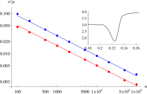
Figure 1: (Color online) Variation coefficient $\sigma/\mu$ for $U_{2}$ (red circles) and $U_{4}$ (blue squares) at $\beta=0.225$ for $L=16$ plotted versus the number of measurements $n$ together with fitted lines with slope $-1/2$. The red line is $0.504/\sqrt{n}$ and blue line is $0.886/\sqrt{n}$. The inset shows the ratio between these two for a range of $\beta$, having the minimum $1.76$ at $\beta=0.225$.

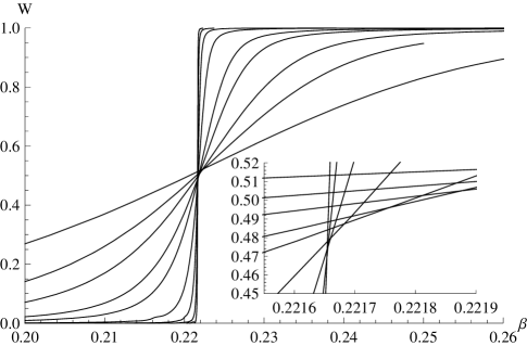
Figure 2: (Color online) $W(\beta,L)$ versus $\beta$ for $L=4$ (smallest slope) to $L=256$ (strongest slope). The inset shows a zoomed in picture near $\beta_{c}$.

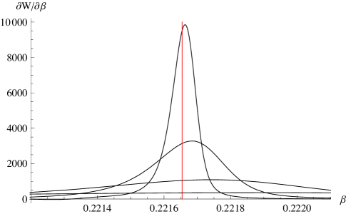
Figure 3: (Color online) $\partial W/\partial\beta$ versus $\beta$ for $L=32,64,128,256$ where the maximum increases with $L$. The red vertical line is located at $\beta_{c}=0.2216541$.

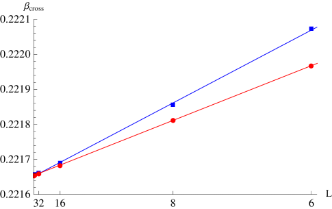
Figure 4: (Color online) Crossing points $\beta_{\mathrm{cross}}$ versus $1/L^{2.40}$ for $L=6,8,16,32,64,128$ for $W$ (red circles) and $g$ (blue squares) and fitted lines.

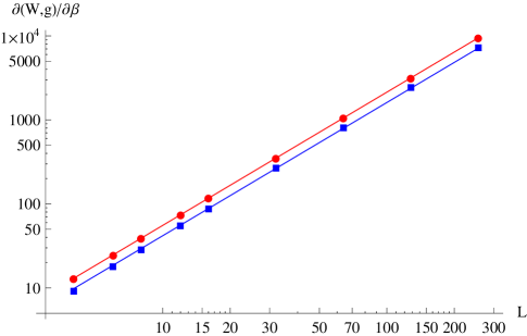
Figure 5: (Color online) Log-log plot of $\partial W/\partial\beta$ (red circles) and $\partial g/\partial\beta$ (blue squares) versus $L$ at $\beta=\beta_{c}=0.2216541$. Lines have slope $1/\nu$.

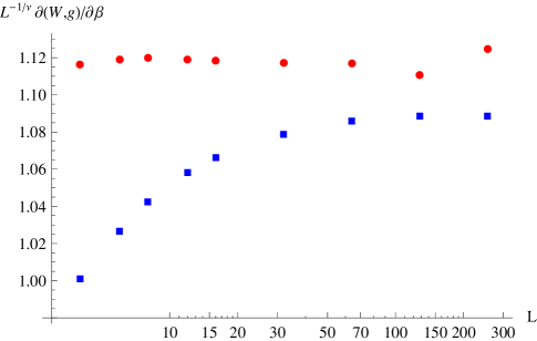
Figure 6: (Color online) $L^{-1/\nu}\,\partial W/\partial\beta-0.32$ (red circles) and $L^{-1/\nu}\,\partial g/\partial\beta$ (blue squares) at $\beta=\beta_{c}=0.2216541$ versus $L$. The $W$-points have been translated by $-0.32$ for easier comparison.

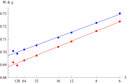
Figure 7: (Color online) $W(\beta_{c},L)+0.22$ (red circles) and $g(\beta_{c},L)$ (blue squares) versus $1/L^{\omega}$ with $\omega=0.814$ for $L=6,8,16,32,64,128,256$. The $W$-points have been translated by $0.22$ for easier comparison.

V The 3d Ising Ferromagnet

The spin-$1/2$ Ising ferromagnet on a simple cubic lattice is an archetypical model system which has been very extensively studied. Although there exist no exact results for any of the critical parameters, $\beta_{c}$ and the critical exponents are known to high precision thanks to RGT theory, high temperature series expansions (HTSE), and numerical simulations (see Refs.  guida:97 ; butera:02 ; deng:03 ). There is consensus that for this system $\beta_{c}\approx 0.221655$, and for the universality class $\nu\approx 0.630$, and $\omega\approx 0.81$. We will test our $W$-data against these values shortly.

We show in Figure 2 an overall view of the behavior of $W(\beta,L)$. It can be seen that on the scale of the figure the curves $W(\beta,L)$ appear to intersect at a unique $L$-independent inverse temperature which can obviously be identified with $\beta_{c}$. The derivatives $\partial W/\partial\beta$ peak strongly at $\beta_{W\!\max}(L)$ which at large $L$ approaches $\beta_{c}$, see Figure 3.

A blow-up of $W(\beta,L)$ in the critical region, Figure 2 inset, shows that there are finite size corrections leading to a weak size dependence of the $[W(\beta,L),W(\beta,2L)]$ crossing points. A plot of the intersection temperatures $\beta_{\mathrm{cross}}$ versus $1/L^{\omega+1/\nu}$, where $\omega+1/\nu\approx 2.40$, is shown in Figure 4 for both $W$ and $g$ (the points for $L=64,128$ are not visible due to the fast data collaps). Fitting a straight line to the $W$-points for $L\geq 6$ versus $1/L^{\omega+1/\nu}$ gives $\beta_{c}=0.2216541(5)$. We have here excluded the point $L=4$ since it appears to deviate from the others in this case. The error estimate is based on how the result depends on excluding a point from the fit and on allowing the exponent $\omega+1/\nu$ to take different values between $2.39$ and $2.41$. In fact, a best fit of the crossing points for $L\geq 6$ to a simple formula $c_{0}+c_{1}\,L^{-\lambda}$ gives on average, taken over fits after excluding one point, $c_{0}\approx 0.2216540(3)$ and $\lambda=2.40(3)$, where the error estimates correspond to the standard deviation of the data set. Since $\nu=0.630$ is known to a higher precision we therefore get $\omega=0.814(30)$ which agrees with previous estimates.

Both of our $\beta_{c}$-estimates are consistent with the most precise values from standard Monte-Carlo simulations $\beta_{c}=0.22165452(8)$ deng:03 , $\beta_{c}=0.2216546(3)$ haggkvist:07 , and from high temperature series analyses, $\beta_{c}=0.221655(2)$ butera:02 . However, the $g$-data seem to require more correction to scaling than the $W$-data. If we want to fit a line to the crossing points for $g$ versus $L^{\omega+1/\nu}$ then we need to drop two more points ($L=6,8$) to get anything like this precision on a $\beta_{c}$-estimate.

Henceforth setting $\beta_{c}=0.2216541$, let us proceed to investigate the derivative data $[\partial W/\partial\beta]_{\beta_{c}}$ and $[\partial g/\partial\beta]_{\beta_{c}}$ against $L$, which are shown as log-log plots in Figure 5. The slopes should be equal to $1/\nu$ in the large $L$ limit. It can be seen that both series of points lie close to $1/0.63$ (slope of the lines).

Let us make a more demanding analysis of the slopes $1/\nu$ by fitting lines to $k$-subsets of the points. Since we have $9$ data points, i.e. we use $L\geq 4$, each $k$ then gives us $\binom{9}{k}$ different slopes. If the data show any sign of inconsistency or a dependency on $L$ then we expect this to show up in the form of different medians and/or different slope intervals. However, we get $\nu=0.6308$ for $k=3,\ldots,9$, with the same value for both median and mean. The quartile deviation of each slope set is about $0.0004$ for $k=4,\ldots,7$. We therefore receive the estimate $\nu=0.6308(4)$. It should be noted that only for the last three points of the $g$-data do we receive a slope that agrees with this estimate.

An alternative way of locating $\beta_{c}$ is to locate the temperature $\beta_{c}$ where the scaling of the derivatives depend least on different $L$. Choosing e.g. subsets of size $k=4$ the narrowest set of slopes is obtained for $\beta_{c}=0.2216541$, give or take a step or two in the last decimal. Since this agrees with our previous two estimates of $\beta_{c}$ we can now give our final estimate of the critical temperature as $\beta_{c}=0.2216541(2)$.

Having established $\beta_{c}$ and $\nu$ we plot the derivatives of $W$ and $g$ in the more demanding form $[\partial W/\partial\beta]_{\beta_{c}}/L^{1/\nu}$ and $[\partial g/\partial\beta]_{\beta_{c}}/L^{1/\nu}$ in Figure 6. The $g$-data clearly show characteristic FSS corrections

$$g(\beta_{c},L)=g(\beta_{c},\infty)\,\left(1+a_{\omega}\,L^{-\omega}+\cdots\right)$$ (13)

at small and moderate $L$ while the $W$-data show only weak and apparently random scatter due to statistical errors, i.e. the analogous correction term for $W(\beta_{c},L)$ appears negligible within the present precision. This means that to extract an estimate of $\nu$ a two parameter fit is sufficient for the $W$ derivative data while a four parameter fit is needed for the $g$-data. This is important as it means that at least in the present case the estimates from $W(\beta_{c},L)$ are intrinsically more precise.

It was estimated in deng:03 that

$$g(\beta_{c},L)=0.69778(13)\,\left(1+0.1788(36)\,L^{-0.82(3)}+\cdots\right)$$ (14)

and our $g$-data, Figure 6, are in excellent agreement with this correction factor for $g(\beta_{c},L)$. We estimate the critical values to be $W(\beta_{c},\infty)=0.468(2)$ and $g(\beta_{c},\infty)=0.697(2)$, see Figure 7, where the error stems from which points are excluded from the fit. The value for $g$ agrees with the formula above but the accuracy is not as good. Also, we would like to mention that at the temperature where the magnetisation distribution shifts from unimodal to bimodal, i.e. where $[\partial^{2}p(m)/\partial m^{2}]_{0}=0$, we found the asymptotic value of $W$ to be about $0.208$ and for $g$ it takes a value near $0.433$.

There are already many accurate estimates of $\nu$ for the $3$d Ising universality group. Renormalization group studies guida:97 give $\nu=0.6304(13)$ and $\nu=0.6305(25)$. The main difficulty concerning either HTSE or MC analyses lies principally with the problem of properly allowing for corrections to scaling. The amplitudes of the corrections vary from system to system, favorizing meta-analyses of data on many systems in the same class. Butera and Comi butera:02 obtain $\nu=0.6299(2)$ from a global analysis of HTSE data for Ising ferromagnets with spin $S$ running from $1/2$ to $\infty$ on both sc and bcc lattices, all systems lying in the same universality class. Their sc $S=1/2$ HTSE results standing alone were consistent with this value but were less accurate ($0.632(2)$ or $0.6277(30)$ depending on the analysis method used). Deng and Blöte deng:03 obtain an entirely independent global estimate $\nu=0.63020(12)$ from simultaneous Monte Carlo analyses on a set of eleven systems all in the same universality class. It is gratifying that the present results on one single system are consistent with and practically as accurate as these global ”best estimates” from HTSE and MC. It would be interesting to establish whether the weak FSS correction for $[\partial W(\beta,L)/\partial\beta]_{\beta_{c}}$ is a general property or is specific to this particular system.

VI Conclusion

We introduce an alternative distribution ”shape” parameter $W(\beta,L)$ for numerical studies of the critical properties of model systems. As an illustration we use this parameter in an analysis of extensive data sets obtained through a density of states technique applied to simple cubic $S=1/2$ Ising ferromagnet samples of size up to $L=256$. In this system at least, corrections to scaling for $W(\beta_{c},L)$ are considerably weaker than those for the canonical Binder cumulant $g(\beta_{c},L)$ and the equilibration time to obtain data to a similar degree of precision is significantly lower. We obtain estimates for the critical inverse temperature $\beta_{c}=0.2216541(2)$ and the critical exponents $\nu=0.6308(4)$ and $\omega=0.814(30)$, based only on $W$-data, which are compatible with and almost as accurate as values from previous Monte Carlo deng:03 and high temperature series expansions butera:02 .

VII Acknowledgements

This research was conducted using the resources of High Performance Computing Center North (HPC2N). We would like to thank Paolo Butera for his invaluable advice.

99

References

- (1) F. J. Wegner, Phys. Rev. B 5, 4529 (1972).
- (2) F. J. Wegner, in Phase Transitions and Critical Phenomena, edited by C. Domb and M. S. Green (Academic Press, New York, 1976), Vol. 6.
- (3) A. Aharony and M. E. Fisher, Phys. Rev. B 27, 4394 (1983).
- (4) V. Privman and M.E. Fisher, Phys. Rev. B 30 322 (1984)
- (5) V. Privman, P.C. Hohenberg and A. Aharony,, in Phase Transitions and Critical Phenomena, edited by C. Domb and J.L. Lebowitz (Academic Press, New York, 1991), Vol. 14.
- (6) J. Salas and A. D. Sokal, J. Stat. Phys. 98, 551 (2000).
- (7) A. Pelissetto and E. Vicari, Phys. Rep. 368, 549 (2002).
- (8) K. Binder, Z. Phys. B Condens. Matter 43 119 (1981).
- (9) F. Wang and D.P. Landau, Phys. Rev. Lett. 86 2050 (2001).
- (10) Jian-Sheng Wang and Robert H. Swendsen, J. Stat. Phys. 106 245 (2002).
- (11) R. Häggkvist, A. Rosengren, D. Andrén, P. Kundrotas, P. H. Lundow and K. Markström, J. Stat. Phys. 114 455 (2004).
- (12) R. Häggkvist, A. Rosengren, P. H. Lundow, K. Markström, D. Andrén and P. Kundrotas, Adv. Phys. 56 653 (2007)
- (13) P. H. Lundow and K. Markström, Cent. Eur. J. Phys., 7 490 (2009)
- (14) R. Guida and J. Zinn-Justin, Nucl. Phys. B 489, 626 (1997), J. Phys. A 31, 8103 (1998).
- (15) P.Butera and M. Comi, Phys. Rev. B, 65 144431 (2002)
- (16) Y. Deng and H.W.J. Blöte, Phys. Rev. E 68 036125 (2003).
99