Fast Correlation Greeks by Adjoint Algorithmic Differentiation

Abstract

We show how Adjoint Algorithmic Differentiation (AAD) allows an extremely efficient calculation of correlation Risk of option prices computed with Monte Carlo simulations. A key point in the construction is the use of binning to simultaneously achieve computational efficiency and accurate confidence intervals. We illustrate the method for a copula-based Monte Carlo computation of claims written on a basket of underlying assets, and we test it numerically for Portfolio Default Options. For any number of underlying assets or names in a portfolio, the sensitivities of the option price with respect to all the pairwise correlations is obtained at a computational cost which is at most 4 times the cost of calculating the option value itself. For typical applications, this results in computational savings of several order of magnitudes with respect to standard methods.

One of the consequences of the current crisis of the Financial Markets is a renewed emphasis on rigorous Risk management practices. In order to quantify the financial exposure of financial firms, and to ensure an efficient capital allocation, and more effective hedging practices, regulators and senior management alike are insisting more and more on a thorough monitoring of Risk. Among all businesses, those dealing with complex, over the counter derivative securities are the ones receiving the most attention.

A thorough calculation of the Risk exposure of portfolios of structured derivatives comes with a high operational cost because of the large amount of computer power required. Indeed, highly time consuming Monte Carlo (MC) simulations are very often the only tool available for pricing and hedging complex securities. Calculating the Greeks, or price sensitivities, by ‘Bumping’ i.e., by perturbing in turn the underlying model parameters, repeating the simulation and forming finite difference approximations results in a computational burden increasing linearly with the number of sensitivities computed. This easily becomes very significant when the models employed depend on a large number of parameters, as it is typically the case.

A particularly challenging task is the calculation of correlation Risk, i.e., the calculation of the sensitivites of a security with respect to some measure of the correlations among the random factors it depends on. Indeed, calculating Risk with respect to all the independent pairwise correlations by Bumping requires repeating the MC simulation a large number of times, e.g. increasing quadratically with the number of random factors, and it is often unfeasible because of its high computational cost.

Several alternative methods for the calculation of price sensitivities have been proposed in the literature (for a review see e.g., Glasserman (2004)). Among these, the Pathwise Derivative method Broadie and Glasserman (1996) provides unbiased estimates at a computational cost that may be smaller than the one of Bumping. However, in many problems the standard Pathwise Derivative method provides limited computational gains, especially when the contract priced has a complex payout Capriotti (in press). A much more efficient implementation of the Pathwise Derivative method was proposed by Giles and Glasserman in Ref. Giles and Glasserman (2006) in the context of the Libor Market Model for European payouts, and recently generalized to Bermudan options by Leclerc and co-workers M. Leclerc and Schneider (2009). These formulations express the calculation of the Pathwise Derivative estimator in terms of linear algebra operations, and utilize adjoint methods to reduce the computational complexity by rearranging appropriately the order of the calculations.

Adjoint implementations can be seen as instances of a programming technique known as Adjoint Algorithmic Differentiation (AAD) Griewank (2000); Giles (2007). In particular, as also discussed in a forthcoming paper Capriotti and Giles (2009), AAD can be used as a design paradigm to implement the Pathwise Derivative method, or the calculation of the sensitivities of any numerical algorithm, in full generality. In this paper we illustrate these ideas by discussing a specific application: the calculation of correlation Risk. We will begin by introducing the main ideas underlying Algorithmic Differentiation (AD), and the results on the computational efficiency of its two basic approaches: the Forward and Adjoint modes.

Forward and Adjoint Algorithmic Differentiation

Both the Forward and Adjoint mode of AD aim at calculating the derivatives of a computer implemented function. They differ by the direction of propagation of the chain rule through the composition of instructions representing the function. To illustrate this point, suppose we begin with a single input $a$, and produce a single output $z$ after proceeding through a sequence of steps:

$$a\ \rightarrow\ \ldots\ \rightarrow\ u\ \rightarrow\ v\ \rightarrow\ \ldots\ \rightarrow\ z.$$

The Forward (or Tangent) mode of AD (FAD) defines $\dot{u}$ to be the sensitivity of $u$ to changes in $a$, i.e.,

$$\dot{u}\equiv\frac{\partial u}{\partial a}~{}.$$

If the intermediate variables $u$ and $v$ are vectors, $\dot{v}$ is calculated by differentiating the dependence of $v$ on $u$ so that

$$\dot{v}_{i}=\sum_{j}\frac{\partial v_{i}}{\partial u_{j}}\ \dot{u}_{j}.$$

Applying this to each step in the calculation, working from left to right, we end up computing $\dot{z}$, the sensitivity of the output to changes in the input. Note that if we have more than one input, then we need to calculate the sensitivity to each one in turn, and so the cost is linear in the number of input variables.

Instead, the Adjoint (or Backward) mode of AD (AAD) works from right to left. Using the standard AD notation, $\bar{u}$ is defined to be the sensitivity of the output $z$ to changes in the intermediate variable $u$, i.e.

$$\bar{u}_{i}\equiv\frac{\partial z}{\partial u_{i}}.$$

Using the chain rule we get,

$$\frac{\partial z}{\partial u_{i}}=\sum_{j}\frac{\partial z}{\partial v_{j}}\ \frac{\partial v_{j}}{\partial u_{i}},$$

which corresponds to the adjoint mode equation

$$\bar{u}_{i}=\sum_{j}\frac{\partial v_{j}}{\partial u_{i}}\ \bar{v}_{j}.$$

Starting from $\bar{z}=1$, we can apply this to each step in the calculation, working from right to left, until we obtain $\bar{a}$, the sensitivity of the output to each of the input variables.

In the Adjoint mode, the cost does not increase with the number of inputs, but if there is more than one output then the sensitivities for each output have to considered one at a time and so the cost is linear in the number of outputs. Furthermore, because the partial derivatives depend on the values of the intermediate variables, one first has to compute the original calculation storing the values of all of the intermediate variables such as $u$ and $v$, before performing the Adjoint mode sensitivity calculation.

In the above description, each step can be a distinct high-level function, or specific mathematical operations, or even an individual instruction in a computer code. This last viewpoint is the one taken by computer scientists who have developed tools which take as an input a computer code to perform some high-level function,

$$V=\texttt{FUNCTION}(U)$$

and produce new routines which will either perform the standard sensitivity analysis

$$\dot{V}=\texttt{FUNCTION}\_{\texttt{D}}(U,\dot{U})$$

with suffix $\_{\texttt{D}}$ for “dot”, or its adjoint counterpart

$$\bar{U}=\texttt{FUNCTION}\_{\texttt{B}}(U,\bar{V})$$

with suffix $\_{\texttt{B}}$ for “bar” .

One particularly important theoretical result is that the number of arithmetic operations in the adjoint routine $\texttt{FUNCTION}\_{\texttt{B}}$ is at most a factor 4 greater than in FUNCTION Griewank (2000). As a result, it is possible to show that the execution time of $\texttt{FUNCTION}\_{\texttt{B}}$ is bounded by approximatively 4 times the cost of execution of the original function FUNCTION. Thus, one can obtain the sensitivity of a single output to an unlimited number of inputs for little more work than the original computation.

While the application of such automatic AD tools to large inhomogeneous pricing softwares is challenging, the principles of AD can be used as a programming paradigm that can be used to design the Forward or Adjoint of any algorithm (possibly using automatic AD tools for the implementation of smaller, simpler components). This is especially useful for the most common situations where pricing codes use a variety of libraries written in different languages, possibly linked dynamically. These ideas will be discussed at length in Ref. Capriotti and Giles (2009).

AAD and the Pathwise Derivative method for Correlation Risk

In this paper, we consider options pricing problems that can be expressed as an expectation value of the form

$$V=\mathbb{E}_{\mathbb{Q}}\Big{[}P(X)\Big{]}~{},$$ (1)

where $X=(X_{1},\ldots,X_{N})^{t}$ represents the state vector of $N$ market factors (e.g., stock prices, interest rates, foreign exchange pairs, default times etc.), $P(X)$ is the (possibly discounted) payout function of a security contingent on their future realization, and $\mathbb{Q}=\mathbb{Q}(X)$ represents a risk neutral probability distribution Harrison and Kreps (1979) according to which the components of $X$ are distributed. Although the proposed method easily generalizes to other kinds of joint distributions, here we consider a $N$-dimensional Gaussian copula as a model for the co-dependence between the components of the state vector, namely a joint cumulative density function of the form

$$\mathbb{Q}(X)=\Phi_{N}(\Phi^{-1}(M_{1}(X_{1})),\ldots,\Phi^{-1}(M_{N}(X_{N}));\rho)$$ (2)

where $\Phi_{N}(Z_{1},\ldots,Z_{N};\rho)$ is a $N$-dimensional multivariate Gaussian distribution with zero mean, and a $N\times N$ positive semidefinite correlation matrix $\rho$; $\Phi^{-1}$ is the inverse of the standard normal cumulative distribution, and $M_{i}(X_{i})$, $i=1,\ldots,N$, are the Marginal distributions of the underlying factors, typically implied from the market prices of liquid securities.

The expectation value in (1) can be estimated by means of MC by sampling a number $N_{\rm MC}$ of random replicas of the underlying state vector ${X}[1],\ldots,{X}[N_{\rm MC}]$, according to the distribution $\mathbb{Q}({X})$, and evaluating the payout $P({X})$ for each of them. This leads to the central limit theorem Kallenberg (1997) estimate of the option value $V$ as

$$V\simeq\frac{1}{N_{\rm MC}}\sum_{i_{\rm MC}=1}^{N_{\rm MC}}P\left({X}[i_{\rm MC}]\right)$$ (3)

with standard error $\Sigma/\sqrt{N_{\rm MC}}$, where $\Sigma^{2}=E_{\mathbb{Q}}[P\left({X}\right)^{2}]-E_{\mathbb{Q}}[P\left(X\right)]^{2}$ is the variance of the sampled payout.

In the Gaussian model above the dependence between the underlying factors is determined by the correlation of a set of jointly normal random variables $Z=(Z_{1},\ldots,Z_{N})^{t}$ distributed according to $\Phi_{N}(Z_{1},\ldots,Z_{N};\rho)$. Each $Z_{i}$ is distributed according to a standard normal distribution so that $\Phi(Z_{i})$ is a uniform random variable in $(0,1)$ and $X_{i}=M_{i}^{-1}(\Phi(Z_{i}))$ is distributed according to $M_{i}$. The sampling of the $N$ jointly normal random variables $(Z_{1},\ldots,Z_{N})$ is efficiently implemented by means of a Cholesky factorization of the correlation matrix. The Cholesky factorization produces a lower triangular $N\times N$ matrix $C$ such that $\rho=CC^{T}$ so that one can write $Z=C\tilde{Z}$ where $\tilde{Z}=(\tilde{Z}_{1},\ldots,\tilde{Z}_{N})^{t}$ is a $N$ dimensional vector of independent standard normal random variables. These observations naturally translate into the standard algorithm to generate MC samples of $X$ according to (2), namely

• Generate a sample of $N$ independent standard normal variates, $\tilde{Z}=(\tilde{Z}_{1},\ldots,\tilde{Z}_{N})^{t}$.

• Correlate the components of $\tilde{Z}$ by performing the matrix vector product $Z=C\tilde{Z}$.

• Set $U_{i}=\Phi(Z_{i})$, $i=1,\ldots,N$.

• Set $X_{i}=M^{-1}(U_{i})$, $i=1,\ldots,N$.

• Compute the payout estimator $P(X_{1},\ldots,X_{N})$.

Correlation Risk can be obtained in an highly efficient way by implementing the so-called Pathwise Derivative method Broadie and Glasserman (1996) according to the principles of AAD Capriotti (in press); Capriotti and Giles (2009). It is convenient to first express the expectation value as being over $\mathbb{P}(\tilde{Z})$, the distribution of independent $\tilde{Z}$ used in the MC simulation, so that

$$V=\mathbb{E_{Q}}\Big{[}P\left({X}\right)\Big{]}=\mathbb{E_{P}}\Big{[}P\left({X(\tilde{Z})}\right)\Big{]}.$$ (4)

The point of this subtle change is that $\mathbb{P}(\tilde{Z})$ does not depend on the correlation matrix $\rho$, whereas $\mathbb{Q}(X)$ does.

The Pathwise Derivative method allows the calculation of the sensitivities of the option price $V$ (4) with respect to a set of $N_{\theta}$ parameter $\theta=(\theta_{1},\ldots,\theta_{N_{\theta}})$, say

$$\frac{\partial V(\theta)}{\partial\theta_{k}}=\frac{\partial}{\partial\theta_{k}}\mathbb{E_{P}}\Big{[}P\left({X}\right)\Big{]}~{},$$ (5)

by defining appropriate estimators, say $\bar{\theta}_{k}(X[i_{MC}])$, that can be sampled simultaneously in a single MC simulation. This can be achieved by observing that whenever the payout function is regular enough (e.g., Lipschitz-continuous, see Ref. Glasserman (2004)), and the distribution $\mathbb{P}(\tilde{Z})$ does not depend on $\theta$, one can rewrite Eq. (5) by taking the derivative inside the expectation value, as

$$\frac{\partial V(\theta)}{\partial\theta_{k}}=\mathbb{E_{P}}\Big{[}\frac{\partial P\left({X}\right)}{\partial\theta_{k}}\Big{]}~{}.$$ (6)

The calculation of Eq. (6) can be performed by applying the chain rule, and computing the average value of the so-called Pathwise Derivative estimator

$$\frac{\partial P(X)}{\partial\theta_{k}}=\sum_{i=1}^{N}\frac{\partial P(X)}{\partial X_{i}}\times\frac{\partial X_{i}}{\partial\theta_{k}}~{}.$$ (7)

The standard pathwise implementation corresponds to a Forward mode sensitivity analysis. Applied to steps 1-4 (since the normal variates $\tilde{Z}$ do not depend on any input parameters), this gives for each sensitivity:

• Calculate $\dot{Z}=\dot{C}\,\tilde{Z}$ where $\dot{C}$ is the sensitivity of $C$ with respect to a given entry of the correlation matrix.

• Set $\dot{U}_{i}=\phi(Z_{i})\,\dot{Z}_{i}$, $i=1,\ldots,N$.

• Set $\dot{X}_{i}=\dot{U}_{i}\,/\,m_{i}(X_{i})$, $i=1,\ldots,N$.

• Calculate $\displaystyle\dot{P}=\sum_{i=1}^{N}\frac{\partial P}{\partial X_{i}}\,\dot{X}_{i}$ .

Here $\phi(x)\equiv{\partial\Phi(x)}/{\partial x}$ is the standard normal probability density function, and $m_{i}(x)\equiv\partial M_{i}(x)/\partial x$ is the probability density function associated with the marginal $M_{i}(x)$ of the $i$-th random factor.

As anticipated, the computational cost of the Forward Pathwise Derivative method scales linearly with the number of sensitivities computed $N_{\theta}$, i.e., the same scaling of finite difference approximations of the derivatives $\partial_{\theta_{k}}E_{\mathbb{Q}}[P(X)]$. As a result in many situations, typically involving complex payouts, the standard implementation of the Pathwise Derivative method offers a limited computational advantage with respect to Bumping Capriotti (in press).

In contrast, AAD allows in general a much more efficient implementation of the Pathwise Derivative estimators (7). Indeed, as an immediate consequence of the computational complexity results introduced in the previous Section, it can be shown Capriotti and Giles (2009) that AAD allows the simultaneous calculation of the Pathwise Derivative estimators for any number of sensitivities at a computational cost which is a small multiple (of order 4) of the cost of evaluating the original payout estimator. As a result, one can calculate the MC expectation of an arbitrarily large number of sensitivities at a small fixed cost.

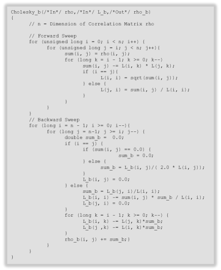
Figure 1: Adjoint of the Cholesky factorization. The Forward sweep is an exact replica of the original factorization.

Although AAD can be applied for virtually any model and payout function of interest in Computational Finance – including path-dependent and Bermudan options – here we will concentrate on the calculation of correlation sensitivities in a Gaussian copula framework. In general, for the reasons mentioned in the previous Section, the AAD implementation of the Pathwise derivative method contains a forward sweep – reproducing the steps followed in the calculation of the estimator of the option value $P(X)$ – and a backward sweep. As a result, the adjoint algorithm consists of adjoint counterparts for each of the Steps 1-4 above executed in reverse order, plus the adjoint of the Cholesky factorization.

The first step consists in the evaluation of the adjoint of step 4 of the Forward sweep, calculating the derivatives of the Payout with respect to the components of the state vector

$$\bar{X}_{k}=\frac{\partial P(X)}{\partial X_{k}}~{},$$ (8)

with $k=1,\ldots,N$. These derivatives can be calculated efficiently using AAD, as discussed in Ref. Capriotti (in press).

In turn, the adjoint of Step 3 of the Forward sweep is given by

$$\bar{U}_{k}=\bar{M}^{-1}_{k}(U_{k},\bar{X}_{k})=\frac{\bar{X}_{k}}{m_{k}(X_{k})}~{},$$ (9)

for $k=1,\ldots,N$. The vector $\bar{U}$ is then mapped into the adjoint of the correlated standard normal variables $\bar{Z}$ through the counterpart of Step 2

$$\bar{Z}_{k}={\bar{\Phi}(Z_{k},\bar{U}_{k})}={\bar{U}_{k}}\,{\phi(Z_{k})}~{}.$$ (10)

The adjoint of Step 1 performing the matrix vector product $Z=C\tilde{Z}$ reads

$$\bar{C}_{i,j}=\sum_{k=1}^{N}\frac{\partial Z_{k}}{\partial C_{i,j}}\,\bar{Z}_{k}=\tilde{Z}_{j}\,\bar{Z}_{i}$$ (11)

or $\bar{C}=\bar{Z}\tilde{Z}^{t}$. By applying the chain rule, it is straightforward to realize that the adjoint $\bar{w}$ of each intermediate variable $w$ in the succession of Steps 0-4 represents the derivative of the Payout estimator with respect to $w$, or $\bar{w}=\partial P/\partial w$. In particular the quantities $\bar{C}_{i,j}$ calculated at the end of the adjoint of Step 1 represent the derivatives of the payout estimator with respect to the the entries of the triangular Cholesky matrix $C$, namely the pathwise estimator (7) with $\theta_{k}=C_{i,j}$.

In summary, the AAD implementation of the Pathwise Derivative Estimator consists of Step 1-4 described above (forward sweep) plus the following steps of the backward sweep:

• Evaluate the Payout adjoint $\bar{X}_{k}=\partial P/\partial X_{k}$, for $k=1,\ldots,N$.

• Calculate $\bar{U}_{k}={\bar{X}_{k}}/{m_{k}(M^{-1}_{k}(U_{k}))}$, $k=1,\ldots,N$.

• Calculate $\bar{Z}_{k}={\bar{U}_{k}}{\phi(Z_{k})}$, $k=1,\ldots,N$.

• Calculate $\bar{C}=\bar{Z}\tilde{Z}^{t}$.

At this point in the calculation, there is an interesting complication. The natural AAD approach would average the values of $\bar{C}$ from each of the MC paths. This average $\bar{C}$ can be converted into derivatives with respect to the entries of the correlation matrix $\rho$ by means of the adjoint of the Cholesky factorization Smith (1995), namely a function of the form

$$\bar{\rho}=\texttt{CHOLESKY}\_\texttt{B}(\rho,\bar{C})$$ (12)

providing

$$\bar{\rho}_{i,j}=\sum_{l,m=1}^{N}\frac{\partial C_{l,m}}{\partial\rho_{i,j}}\bar{C}_{l,m}~{}.$$ (13)

The pseudocode for the adjoint Cholesky factorization is given in Fig. 1. By inspecting the structure of the pseudocode it appears clear that its computational cost is just a small multiple (of order 2) of the cost of evaluating the original factorization. Indeed, the adjoint algorithm essentially contains the original Cholesky factorization plus a backward sweep with the same complexity and a similar number of operations.

The complication with this implementation is that it gives an estimate for the correlation risk, but it does not provide a corresponding confidence interval. An alternative approach would be to convert $\bar{C}$ to $\bar{\rho}$ for each individual path, and then compute the average and standard deviation of $\bar{\rho}$ in the usual way. However, the numerical results will show that this is rather costly. An excellent compromise between these two extremes is to divide the $N_{MC}$ paths into $N_{b}$ ’bins’ of equal size. For each bin, an average value of $\bar{C}$ is computed and converted into a corresponding value for $\bar{\rho}$. These $N_{b}$ estimates for $\bar{\rho}$ can then be combined in the usual way to form an overall estimate and confidence interval for the correlation risk.

The computational benefits can be understood by considering the computational costs for both the standard evaluation and the adjoint Pathwise Derivative calculation. In the standard evaluation, the cost of the Cholesky factorization is $O(N^{3})$, and the cost of the MC sampling is $O(N_{MC}N^{2})$, so the total cost is $O(N^{3}+N_{MC}N^{2})$. Since $N_{MC}$ is always much greater than $N$, the cost of the Cholesky factorization is usually negligible. The cost of the adjoint steps in the MC sampling is also $O(N_{MC}N^{2})$, and when using $N_{b}$ bins the cost of the adjoint Cholesky factorization is $O(N_{b}N^{3})$. To obtain an accurate confidence interval, but with the cost of the Cholesky factorisation being negligible, requires that $N_{b}$ is chosen so that $1\ll N_{b}\ll N_{MC}/N$. Without binning, i.e., using $N_{b}=N_{MC}$, the cost to calculate the average of the estimators (13) is $O(N_{MC}N^{3})$, and so the relative cost compared to the evaluation of the option value is $O(N)$.

Figure 2: Ratios of the CPU time required for the calculation of the option value, and correlation Greeks, and the CPU time spent for the computation of the value alone, as functions of the number of names in the basket, for $N_{MC}=10^{5}$. Symbols: Bumping (one-sided finite differences) (triangles), AAD without binning (i.e. $N_{b}=N_{MC}$) (stars), AAD with binning ($N_{b}=20$) (empty circles). Lines are guides for the eye, and the MC uncertainties are smaller than the symbol sizes.

The binning procedure described above can be generalized to any situation in which the standard solution procedure involves a common preprocessing step before any of the path calculations are performed. Other examples would include calibration of model parameters to market prices, or a cubic spline construction of a local volatility surface. In each case, there is a linear relationship between the forward mode sensitivities before and after the preprocessing step, and therefore a linear relationship between the corresponding adjoint sensitivities.

The algorithm described above can be applied whenever the option pricing problem can be formulated as an expectation value over a set of random factors whose distribution is modelled as a Gaussian copula. This include in general a variety of Basket Options common across all asset classes, or structured swaps whose coupon depends on a specific observation of a set of correlated rates. In addition, the same ideas can be extended to the simulation of correlated diffusion processes Capriotti and Giles (2009).

Numerical Tests

As a numerical test ground we consider the case of Basket Default Options Chen and Glasserman (2008). In this context, the random factors $X_{i}$ represent the default time $\tau_{i}$ of the $i$-th name, e.g., the time a specific company in a reference pool of $N$ names fails to pay one of its liabilities as specified by the terms of the contract priced. In particular, in a $n$-th to default Basket Default Swap one party (protection buyer) makes regular payments to a counterparty (protection seller) at time $T_{1},\ldots,T_{M}\leq T$ provided that less than $n$ defaults events among the components of the basket are observed before time $T_{M}$. On the other hand, if $n$ defaults occur before time $T$, the regular payments cease and the protection seller makes a payment to the buyer of $(1-R_{i})$ per unit notional, where $R_{i}$ is the normalized recovery rate of the $i$-th asset. The value at time zero of the Basket Default Swap on a given realization of the default times $\tau_{1},\ldots,\tau_{N}$, i.e., the Payout function, can be therefore expressed as

$$P(\tau_{1},\ldots,\tau_{N})=P_{prot}(\tau_{1},\ldots,\tau_{N})-P_{prem}(\tau_{1},\ldots,\tau_{N})$$ (14)

i.e., as the difference between the so-called protection and premium legs. The value leg is given by

$$P_{prot}(\tau_{1},\ldots,\tau_{N})=(1-R_{n})D(\tau)\mathbb{I}(\tau\leq T)~{},$$ (15)

where $R_{n}$ and $\tau$ are the recovery rate and default time of the $n$-th to default, respectively, $D(t)$ is the discount factor for the interval $[0,t]$ (here we assume for simplicity uncorrelated default times and interest rates), and ${\mathbb{I}}(\tau\leq T)$ is the indicator function of the event that the $n$-th default occurs before $T$. The premium leg reads instead, neglecting for simplicity any accrued payment,

$$P_{prem}(\tau_{1},\ldots,\tau_{N})=\sum_{k=1}^{L(\tau)}s_{k}D(T_{k})$$ (16)

where $L(\tau)=\max[k\in\{1,\ldots,M\}/T_{k}<\tau]$, and $s_{k}$ is the premium payment (per unit notional) at time $T_{k}$.

In order to apply the Pathwise Derivative method to the payout above, the indicator functions in (16) and (15), need to be regularized Glasserman (2004); Chen and Glasserman (2008). One simple and practical way of doing that is to replace the indicator functions with their smoothed counterpart, at the price of introducing a small amount of bias in the Greek estimators. For the problem at hand, as it is also generally the case, such bias can be easily reduced to be smaller than the statistical errors that can be obtained for any realistic number of MC iteration $N_{MC}$ (for a more complete discussion of the topic of payout regularization see Refs. Capriotti (in press); Capriotti and Giles (2009); Giles (2009)).

The remarkable computational efficiency of AAD is illustrated in Fig. 2 for the Second to Default Swap. Here we plot the ratio of the CPU time required for the calculation of the value of the option, and all its pairwise correlation sensitivities, and the CPU time spent for the computation of the value alone, as functions of the number of names in the basket. As expected, for standard finite-difference estimators, such ratio increases quadratically with the number of names in the basket. Already for medium sized basket ($N\simeq 20$) the cost associated with Bumping is over 100 times more expensive than the one of AAD.

Nevertheless, at a closer look (see the inset of Fig. 2), the relative cost of AAD without binning is $O(N)$, for the reasons explained earlier. However, when using $N_{b}=20$ bins the cost of the adjoint Cholesky computation is negligible and the numerical results show that all the Correlation Greeks can be obtained with a mere 70% overhead compared to the calculation of the value of the option. This results in over 2 orders of magnitude savings in computational time for a basket of over 40 Names.

Conclusions

In conclusion, we have shown how Adjoint Algorithmic Differentiation allows an extremely efficient calculation of correlation Risk in Monte Carlo. The proposed method relies on using the Adjoint mode of Algorithmic Differentiation to organize the calculation of the Pathwise Derivative estimator, and to implement the adjoint counterpart of the Cholesky factorization. For any number of underlying assets or names in a portfolio, the proposed method allows the calculation of the complete pairwise correlation Risk at a computational cost which is at most 4 times the cost of calculating the option value itself, resulting in remarkable computational savings with respect to Bumping. We illustrated the method for a Gaussian copula-based Monte Carlo computation, and we tested it numerically for Portfolio Default Options. In this application, the proposed method is 100 times faster than Bumping for 20 names, and over 1000 times for 40 names. The method generalizes immediately to other kind of Elliptic copulas, and to a general diffusive setting. In fact, it is a specific instance of a general AAD approach to the implementation of the Pathwise Derivative method that will be discussed in a forthcoming publication Capriotti and Giles (2009).

Acknowledgments: It is a pleasure to acknowledge useful discussions with Alex Prideaux, Adam and Matthew Peacock, Jacky Lee and David Shorthouse. Valuable help provided by Mark Bowles and Anca Vacarescu in the initial stages of this project is also gratefully acknowledged. The opinions and views expressed in this paper are uniquely those of the authors, and do not necessarily represent those of Credit Suisse Group.

References

- Glasserman (2004) P. Glasserman, Monte Carlo Methods in Financial Engineering (Springer, New York, 2004).
- Broadie and Glasserman (1996) M. Broadie and P. Glasserman, Management Science 42, 269 (1996).
- Capriotti (in press) L. Capriotti, Journal of Computational Finance (in press).
- Giles and Glasserman (2006) M. Giles and P. Glasserman, Risk 19, 88 (2006).
- M. Leclerc and Schneider (2009) Q. M. Leclerc and I. Schneider, Risk 22, 84 (2009).
- Griewank (2000) A. Griewank, Evaluating Derivatives: Principles and Techniques of Algorithmic Differentiation (Frontiers in Applied Mathematics, Philadelphia, 2000).
- Giles (2007) M. Giles, Proceedings of HERCMA conference (2007).
- Capriotti and Giles (2009) L. Capriotti and M. Giles, in preparation (2009).
- Harrison and Kreps (1979) J. Harrison and D. Kreps, Journal of Economic Theory 20, 381 (1979).
- Kallenberg (1997) O. Kallenberg, Foundations of Modern Probability (Springer, New York, 1997).
- Smith (1995) S. P. Smith, Journal of Computational and Graphic Statistics 4, 134 (1995).
- Chen and Glasserman (2008) Z. Chen and P. Glasserman, Finance and Stochastics 12, 507 (2008).
- Giles (2009) M. Giles, in Monte Carlo and Quasi-Monte Carlo Methods, edited by P. L. Ecuyer and A. B. Owen (Springer, 2009).