Distributed anonymous discrete function computation and averaging

Abstract

We propose a model for deterministic distributed function computation by a network of identical and anonymous nodes. In this model, each node has bounded computation and storage capabilities that do not grow with the network size. Furthermore, each node only knows its neighbors, not the entire graph. Our goal is to characterize the class of functions that can be computed within this model. In our main result, we provide a necessary condition for computability which we show to be nearly sufficient, in the sense that every function that violates this condition can at least be approximated. The problem of computing (suitably rounded) averages in a distributed manner plays a central role in our development; we provide an algorithm that solves it in time that grows quadratically with the size of the network.

1 Introduction

The goal of many multi-agent systems, distributed computation algorithms, and decentralized data fusion methods is to have a set of nodes compute a common value based on initial values or observations at each node. Towards this purpose, the nodes, which we will sometimes refer to as agents, perform some internal computations and repeatedly communicate with each other. The objective of this paper is to understand the fundamental limitations and capabilities of such systems and algorithms when the available information and computational resources at each node are limited.

1.1 Motivation

The model that we will employ is a natural one for many different settings, including the case of wireless sensor networks. However, before describing the model, we start with a few examples that motivate the questions that we address.

(a) Quantized consensus: Suppose that each node begins with an integer value $x_{i}(0){\in\{0,\ldots,K\}}$. We would like the nodes to end up, at some later time, with values $y_{i}$ that are almost equal, i.e., $|y_{i}-y_{j}|\leq 1$, for all $i,j$, while preserving the sum of the values, i.e., $\sum_{i=1}^{n}x_{i}(0)=\sum_{{i=1}}^{n}y_{i}$. This is the so-called quantized averaging problem, which has received considerable attention recently; see, e.g., [20, 13, 3, 24, 7]. It may be viewed as the problem of computing the function $(1/n)\sum_{i=1}^{n}x_{i}$, rounded to an integer value.

(b) Distributed hypothesis testing and majority voting: Consider $n$ sensors interested in deciding between two hypotheses, $H_{0}$ and $H_{1}$. Each sensor collects measurements and makes a preliminary decision $x_{i}\in\{0,1\}$ in favor of one of the hypotheses. The sensors would like to make a final decision by majority vote, in which case they need to compute the indicator function of the event $\sum_{i=1}^{n}x_{i}\geq n/2$, in a distributed way. Alternatively, in a weighted majority vote, they may be interested in computing the indicator function of an event such as $\sum_{i=1}^{n}x_{i}\geq 3n/4$. A variation of this problem involves the possibility that some sensors abstain from the vote, perhaps due to their inability to gather sufficiently reliable information.

(c) Direction coordination on a ring: Consider $n$ vehicles placed on a ring, each with some arbitrarily chosen direction of motion (clockwise or counterclockwise). We would like the $n$ vehicles to agree on a single direction of motion. A variation of this problem was considered in [29], where, however, additional requirements on the vehicles were imposed which we do not consider here. The solution provided in [29] was semi-centralized in the sense that vehicles had unique numerical identifiers, and the final direction of most vehicles was set to the direction of the vehicle with the largest identifier. We wonder whether the direction coordination problem can be solved in a completely decentralized way. Furthermore, we would like the final direction of motion to correspond to the initial direction of the majority of the vehicles: if, say, 90% of the vehicles are moving counterclockwise, we would like the other 10% to turn around. If we define $x_{i}$ to be $1$ when the $i$th vehicle is initially oriented clockwise, and $0$ if it is oriented counterclockwise, then, coordinating on a direction involves the distributed computation of the indicator function of the event $\sum_{i=1}^{n}x_{i}\geq n/2$.

(d) Solitude verification: This is the problem of checking whether exactly one node has a given state. This problem is of interest if we want to avoid simultaneous transmissions over a common channel [17], or if we want to maintain a single leader (as in motion coordination — see for example [19]) Given states $x_{i}\in\{{0},1,\ldots,{K}\}$, solitude verification is equivalent to the problem of computing the binary function which is equal to 1 if and only if $|\{i:x_{i}={0}\}|=1$.

There are numerous methods that have been proposed for solving problems such as the above; see for example the vast and growing literature on consensus and averaging methods, or the distribute robotics literature [9]. Oftentimes, different algorithms involve different computational capabilities on the part of the nodes, which makes it hard to talk about a “best” algorithm. At the same time, simple algorithms (such as setting up a spanning tree and aggregating information by progressive summations over the tree) are often considered undesirable because they require too much coordination or global information. It should be clear that a sound discussion of such issues requires the specification of a precise model of computation, followed by a systematic analysis of fundamental limitations under a given model. This is precisely the objective of this paper: to propose a particular model, and to characterize the class of functions computable under this model.

1.2 The features of our model

Our model provides an abstraction for common requirements for distributed algorithms in the wireless sensor network literature. We model the nodes as interacting deterministic finite automata that exchange messages on a fixed bidirectional network, with no time delays or unreliable transmissions. Some important qualitative features of our model are the following.

Identical nodes: Any two nodes with the same number of neighbors must run the same algorithm. Note that this assumption is equivalent to assuming that the nodes are exactly identical. Any algorithm that works in this setting will also work if the nodes are not all identical, since the nodes can still run the same algorithm.

Anonymity: A node can distinguish its neighbors using its own, private, local identifiers. However, nodes do not have global identifiers. In other words, a node receiving a message from one of its neighbors can send an answer to precisely that neighbor, or recognize that a later message comes from this same neighbor. On the other hand, nodes do not a priori have a unique signature that can be recognized by every other node.

Determinism: Randomization is not allowed. This restriction is imposed in order to preclude essentially centralized solutions that rely on randomly generated distinct identifiers and thus bypass the anonymity requirement. Clearly, developing algorithms is much harder, and sometimes impossible, when randomization is disallowed.

Limited memory: We focus on the case where the nodes can be described by finite automata, and pay special attention to the required memory size. Ideally, the number of memory bits required at each node should be bounded above by a slowly growing function of the degree of a node.

Absence of global information: Nodes have no global information, and do not even have an upper bound on the total number of nodes. Accordingly, the algorithm that each node is running is independent of the network size and topology.

Convergence requirements: Nodes hold an estimated output that must converge to a desired value which is a function of all nodes’ initial observations or values. In particular, for the case of discrete outputs, all nodes must eventually settle on the desired value. On the other hand, the nodes do not need to become aware of such termination, which is anyway impossible in the absence of any global information [6].

In this paper, we only consider the special case of fixed graph topologies, where the underlying (and unknown) interconnection graph does not change with time. Developing a meaningful model for the time-varying case and extending our algorithms to that case is an interesting topic, but outside the scope of this paper.

1.3 Literature review

There is a very large literature on distributed function computation in related models of computation [8, 25]. This literature can be broadly divided into two strands, although the separation is not sharp: works that address general computability issues for various models, and works that focus on the computation of specific functions, such as the majority function or the average. We start by discussing the first strand.

A common model in the distributed computing literature involves the requirement that all processes terminate once the desired output is produced and that nodes become aware that termination has occurred. A consequence of the termination requirement is that nodes typically need to know the network size $n$ (or an upper bound on $n$) to compute non-trivial functions. We refer the reader to [1, 6, 36, 21, 31] for some fundamental results in this setting, and to [14] for a comprehensive summary of known results. Closest to our work is the reference [11] which provides an impossibility result very similar to our Theorem 3.1, for a closely related model computation.

The biologically-inspired “population algorithm” model of distributed computation has some features in common with our model, namely, anonymous, bounded-resource nodes, and no requirement of termination awareness; see [2] for an overview of available results. However, this model involves a different type of node interactions from the ones we consider; in particular, nodes interact pairwise at times that may be chosen adversarially.

Regarding the computation of specific functions, [26] shows the impossibility of majority voting if the nodes are limited to a binary state. Some experimental memoryless algorithms (which are not guaranteed to always converge to the correct answer) have been proposed in the physics literature [16]. Several papers have quantified the performance of simple heuristics for computing specific functions, typically in randomized settings. We refer the reader to [18], which studied simple heuristics for computing the majority function, and to [34], which provides a heuristic that has guarantees only for the case of complete graphs.

The large literature on quantized averaging often tends to involve themes similar to those addressed in this paper [13, 24, 3, 10, 20]. However, the underlying models of computation are typically more powerful than ours, as they allow for randomization and unbounded memory. Closer to the current paper, [32] develops an algorithm with $O(n^{2})$ convergence time for a variant of the quantized averaging problem, but requires unbounded memory. Reference [7] provides an algorithm for the particular quantized averaging problem that we consider in Section 4 (called in [7] the “interval consensus problem”), which uses randomization but only bounded memory (a total of two bits at each node). An upper bound on its expected convergence time is provided in [12] as a function of $n$ and a spectral quantity related to the network. A precise convergence time bound, as a function of $n$, is not given. Similarly, the algorithm in [37] runs in $O(n^{5})$ time for the case of fixed graphs. (However, we note that [37] also addresses an asynchronous model involving time-varying graphs.) Roughly speaking, the algorithms in [7, 37] work by having positive and negative “load tokens” circulate randomly in the network until they meet and annihilate each other. Our algorithm involves a similar idea. However, at the cost of some algorithmic complexity, our algorithm is deterministic. This allows for fast progress, in contrast to the slow progress of algorithms that need to wait until the coalescence time of two independent random walks. Finally, a deterministic algorithm for computing the majority function (and some more general functions) was proposed in [28]. However, the algorithm appears to rely on the computation of shortest path lengths, and thus requires unbounded memory at each node.

Semi-centralized versions of the problem, in which the nodes ultimately transmit to a fusion center, have often been considered in the literature, e.g., for distributed statistical inference [30] or detection [23]. The papers [15], [22], and [27] consider the complexity of computing a function and communicating its value to a sink node. We refer the reader to the references therein for an overview of existing results in such semi-centralized settings. However, the underlying model is fundamentally different from ours, because the presence of a fusion center violates our anonymity assumption.

Broadly speaking, our results differ from previous works in several key respects: (i) Our model, which involves totally decentralized computation, deterministic algorithms, and constraints on memory and computation resources at the nodes, but does not require the nodes to know when the computation is over, is different from that considered in almost all of the relevant literature. (ii) Our focus is on identifying computable and non-computable functions under our model, and we achieve a nearly tight separation, as evidenced by a comparison between Theorem 3.1 and Corollary 4.3. (iii) Our $O(n^{2})$ averaging algorithm is quite different, and significantly faster than available memory-limited algorithms.

1.4 Summary and Contributions

We provide a general model of decentralized anonymous computation on fixed graphs, with the features described in Section 1.2, and characterize the type of functions of the initial values that can be computed.

We prove that if a function is computable under our model, then its value can only depend on the frequencies of the different possible initial values. For example, if the initial values $x_{i}$ are binary, a computable function can only depend on $p_{0}:=|\{i:x_{i}=0\}|/n$ and $p_{1}:=|\{i:x_{i}=1\}|/n$. In particular, determining the number of nodes, or whether at least two nodes have an initial value of $1$, is impossible.

Conversely, we prove that if a function only depends on the frequencies of the different possible initial values (and is measurable), then the function can be approximated with any given precision, except possibly on a set of frequency vectors of arbitrarily small volume. Moreover, if the dependence on these frequencies can be expressed through a combination of linear inequalities with rational coefficients, then the function is computable exactly. In particular, the functions involved in the quantized consensus, distributed hypothesis testing, and direction coordination examples are computable, whereas the function involved in solitude verification is not. Similarly, statistical measures such as the standard deviation of the distribution of the initial values can be approximated with arbitrary precision. Finally, we show that with infinite memory, the frequencies of the different initial values (i.e., $p_{0}$, $p_{1}$ in the binary case) are computable exactly, thus obtaining a precise characterization of the computable functions in this case.

The key to our positive results is a new algorithm for calculating the (suitably quantized) average of the initial values, which is of independent interest. The algorithm does not involve randomization, requires only $O(n^{2})$ time to terminate, and the memory (number of bits) required at each node is only logarithmic in the node’s degree. In contrast, existing algorithms either require unbounded memory, or are significantly slower to converge.

1.5 Outline

In Section 2, we describe formally our model of computation. In Section 3, we establish necessary conditions for a function to be computable. In Section 4, we provide sufficient conditions for a function to be computable or approximable. Our positive results rely on an algorithm that keeps track of nodes with maximal values, and an algorithm that calculates a suitably rounded average of the nodes’ initial values; these are described in Sections 5 and 6, respectively. We provide some corroborating simulations in Setion 7, and we end with some concluding remarks, in Section 8.

2 Formal description of the model

Under our model, a distributed computing system consists of three elements:

(a) A network: A network is a triple $(n,G,{\cal L})$, where $n$ is the number of nodes, and $G=(V,E)$ is a connected bidirectional graph $G=(V,E)$ with $n$ nodes. (By bidirectional, we mean that the graph is directed but if $(i,j)\in E$, then $(j,i)\in E$.) We define $d(i)$ as the in-degree (and also out-degree, hence “degree” for short) of node $i$. Finally, $\cal L$ is a port labeling which assigns a port number (a distinct integer in the set $\{{0,1,}\ldots,d(i)\}$) to each outgoing edge of any node $i$. Note that the unique identifiers $i$ used to refer to nodes are only introduced for the purpose of analysis, and are not part of the actual system. In particular, nodes do not know and cannot use their identifiers.

(b) Input and output sets: The input set is a finite set $X=\{0,1,\ldots,K\}$ to which the initial value of each node belongs. The output set is a finite set $Y$ to which the output of each node belongs.

(c) An algorithm: An algorithm is defined as a family of finite automata $(A_{d})_{d=1,2,\ldots}$, where the automaton $A_{d}$ describes the behavior of a node with degree $d$. The state of the automaton $A_{d}$ is a tuple ${[}x,z,y;(m_{1},\ldots,m_{d})]$; we will call $x\in X$ the initial value, $z\in{Z_{d}}$ the internal memory state, $y\in Y$ the output or estimated answer, and $m_{1},\ldots,m_{d}\in M$ the outgoing messages. The sets $Z_{d}$ and $M$ are assumed finite. We allow the cardinality of $Z_{d}$ to increase with $d$. Clearly, this would be necessary for any algorithm that needs to store the messages received in the previous time step. Each automaton $A_{d}$ is identified with a transition law from $X\times{Z_{d}}\times Y\times M^{d}$ into itself, which maps each $\left[x,z,y;(m_{1},\dots,m_{d})\right]$ to some $\left[x,z^{\prime},y^{\prime};(m^{\prime}_{1},\dots,m^{\prime}_{d})\right].$ In words, at each iteration, the automaton takes $x$, $z$, $y$, and incoming messages into account, to create a new memory state, output, and (outgoing) messages, but does not change the initial value.

Given the above elements of a distributed computing system, an algorithm proceeds as follows. For convenience, we assume that the above defined sets $Y$, $Z_{d}$, and $M$ contain a special element, denoted by $\emptyset$. Each node $i$ begins with an initial value $x_{i}\in X$ and implements the automaton $A_{d(i)}$, initialized with $x=x_{i}$ and $z=y=m_{1}=\cdots=m_{d}=\emptyset$. We use $S_{i}(t)=[{x_{i}},y_{i}(t),z_{i}(t),m_{i,1}(t),\ldots,m_{i,d(i)}(t)]$ to denote the state of node $i$’s automaton at time $t$. Consider a particular node $i$. Let $j_{1},\ldots,j_{d(i)}$ be an enumeration of its neighbors, according to the port numbers. (Thus, $j_{k}$ is the node at the other end of the $k$th outgoing edge at node $i$.) Let $p_{k}$ be the port number assigned to link $(j_{k},i)$ according to the port labeling at node $j_{k}$. At each time step, node $i$ carries out the following update:

$$\left[x_{i},z_{i}(t+1),y_{i}(t+1);m_{i,1}(t+1),\ldots,m_{i,d(i)}({t+1})\right]=A_{d(i)}\left[{x_{i}},z_{i}(t),y_{i}(t);m_{{j_{1},p_{1}}}(t),\ldots,m_{j_{d{(i)}},p_{d{{(i)}}}}(t)\right].$$

In words, the messages $m_{j_{k},p_{k}}(t)$, $k=1,\ldots,d(i)$, “sent” by the neighbors of $i$ into the ports leading to $i$ are used to transition to a new state and create new messages $m_{i,k}(t+1)$, $k=1,\ldots,d(i)$, that $i$ “sends” to its neighbors at time $t+1$. We say that the algorithm terminates if there exists some $y^{*}\in Y$ (called the final output of the algorithm) and a time $t^{\prime}$ such that $y_{i}(t)=y^{*}$ for every $i$ and $t\geq t^{\prime}$.

Consider now a family of functions $(f_{n})_{n=1,2,\ldots}$, where $f_{n}:X^{n}\to Y$. We say that such a family is computable if there exists a family of automata $(A_{d})_{d=1,2,\ldots}$ such that for any $n$, for any network $(n,G,{\cal L})$, and any set of initial conditions $x_{1},\dots,x_{{n}}$, the resulting algorithm terminates and the final output is $f_{{n}}(x_{1},\dots,x_{n})$. Intuitively, a family of functions is computable if there is a bounded-memory algorithm which allows the nodes to “eventually” learn the value of the function in any connected topology and for any initial conditions.

As an exception to the above definitions, we note that although we primarily focus on the finite case, we will briefly consider in Section 4 function families $(f_{n})_{n=1,2,\ldots}$ computable with infinite memory, by which we mean that the internal memory sets $Z_{d}$ and the output set $Y$ are countably infinite, the rest of the model remaining the same.

The rest of the paper focuses on the following general question: what families of functions are computable, and how can we design a corresponding algorithm $(A_{d})_{d=1,2,\ldots}$? To illustrate the nature of our model and the type of algorithms that it supports, we provide a simple example.

Detection problem: In this problem, all nodes start with a binary initial value $x_{i}\in\{0,1\}=X$. We wish to detect whether at least one node has an initial value equal to $1$. We are thus dealing with the function family $(f_{n})_{n=1,2,\ldots}$, where $f_{n}(x_{1},\ldots,x_{n})=\max\{x_{1},\ldots,x_{n}\}$. This function family is computable by a family of automata with binary messages, binary internal state, and with the following transition rule:

  if $x_{i}=1$ or $z_{i}(t)=1$ or ${\max}_{j:(i,j)\in E}m_{ji}(t)=1$ then

        set $z_{i}(t+1)=y_{i}(t+1)=1$

        send $m_{ij}(t+1)=1$ to every neighbor $j$ of $i$

  else

        set $z_{i}(t+1)=y_{i}(t+1)=0$

        send $m_{ij}(t+1)=0$ to every neighbor $j$ of $i$

  end if

In the above algorithm, we initialize by setting $m_{ij}(0)$, $y_{i}(0)$, and $z_{i}(0)$ to zero instead of the special symbol $\emptyset$. One can easily verify that if $x_{i}=0$ for every $i$, then $y_{i}(t)=0$ for all $i$ and $t$. If on the other hand $x_{k}=1$ for some $k$, then at each time step $t$, those nodes $i$ at distance less than $t$ from $k$ will have $y_{i}(t)=1$. Thus, for connected graphs, the algorithm will terminate within $n$ steps, with the correct output. It is important to note, however, that because $n$ is unknown, a node $i$ can never know whether its current output $y_{i}(t)$ is the final one. In particular, if $y_{i}(t)=0$, node $i$ cannot exclude the possibility that $x_{k}=1$ for some node whose distance from $i$ is larger than $t$.

3 Necessary condition for computability

In this section we establish our main negative result, namely, that if a function family is computable, then the final output can only depend on the frequencies of the different possible initial values. Furthermore, this remains true even if we allow for infinite memory, or restrict to networks in which neighboring nodes share a common label for the edges that join them. This result is quite similar to Theorem 3 of [11], and so is the proof. Nevertheless, we provide a proof in order to keep the paper self-contained.

We first need some definitions. Recall that $X=\{0,1,\ldots,K\}$. We let $D$ be the unit simplex, that is, $D=\{({p_{0}},\dots,p_{K})\in[0,1]^{{K+1}}:\sum_{k={0}}^{K}p_{k}=1\}$. We say that a function $h:D\to Y$ corresponds to a function family $(f_{n})_{n=1,2,\ldots}$ if for every $n$ and every $x\in{X}^{n}$, we have

$$f(x_{1},\dots,x_{n})=h\left({p_{0}}(x_{1},\ldots,x_{n}),p_{1}(x_{1},\ldots,x_{n}),\dots,p_{K}(x_{1},\ldots,x_{n})\right),$$

where

$$p_{k}(x_{1},\ldots,x_{n})=|\{{i}~{}|~{}x_{{i}}={k}\}|/n,$$

so that $p_{k}(x_{1},\ldots,x_{n})$ is the frequency of occurrence of the initial value $k$. In this case, we say that the family $(f_{n})$ is frequency-based. Note that $n$ is used in defining the notion of frequency, but its value is unknown to the agents, and cannot be used in the computations.

Theorem 3.1.

Suppose that the family $(f_{n})$ is computable with infinite memory. Then, this family is frequency-based. The result remains true even if we only require computability over edge-labeled networks.

The following are some applications of Theorem 3.1.

(a)  The parity function $\sum_{i=1}^{n}x_{i}~{}({\rm mod}\ k)$ is not computable, for any $k>{1}$.

(b)  In a binary setting $(X=\{0,1\})$, checking whether the number of nodes with $x_{i}=1$ is larger than or equal to the number of nodes with $x_{i}=0$ plus 10 is not computable.

(c)  Solitude verification, i.e., checking whether $|i:\{x_{i}=0\}|=1$, is not computable.

(d)  An aggregate difference function such as $\sum_{i<j}|x_{i}-x_{j}|$ is not computable, even if it is to be calculated modulo $k$.

3.1 Proof of Theorem 3.1

The proof of Theorem 3.1 involves a particular degree-two network (a ring), in which all port numbers take values in the set $\{{0},1,2\}$, and in which any two edges $(i,j)$ and $(j,i)$ have the same port number, as represented in Fig. 1. More precisely, it relies on showing that two rings obtained by repeating, respectively, $k$ and $k^{\prime}$ times the same sequences of nodes, edges, and initial conditions are algorithmically indistinguishable, and that any computable family of functions must thus take the same value on two such rings. The proof proceeds through a sequence of intermediate results, starting with the following lemma, which essentially reflects the fact that the node identifiers used in our analysis do not influence the course of the algorithm. It can be easily proved by induction on time, and its proof is omitted. The second lemma states that the value taken by computable (families of) functions may not depend on which particular node has which initial condition.

Lemma 3.1.

Suppose that $G=(\{1,\ldots,n\},E)$ and $G^{\prime}=(\{1,\ldots,n\},E^{\prime})$ are isomorphic; that is, there exists a permutation $\pi$ such that $(i,j)\in E$ if and only if $(\pi(i),\pi(j))\in E^{\prime}$. Furthermore, suppose that the port label at node $i$ for the edge leading to $j$ in $G$ is the same as the port label at node $\pi(i)$ for the edge leading to $\pi(j)$ in $G^{\prime}$. Then, the state $S_{i}(t)$ resulting from the initial values $x_{1},\ldots,x_{n}$ on the graph $G$ is the same as the state $S_{\pi(i)}(t)$ resulting from the initial values $x_{{\pi^{-1}}(1)},\ldots,x_{{\pi^{-1}}(n)}$ on the graph $G^{\prime}$.

Lemma 3.2.

Suppose that the family $(f_{n})_{n=1,2,\ldots}$ is computable with infinite memory on edge-labeled networks. Then, each $f_{i}$ is invariant under permutations of its arguments.

Proof.

Let ${\pi_{ij}}$ be the permutation that swaps $i$ with $j$ (leaving the other nodes intact); with a slight abuse of notation, we also denote by $\pi_{ij}$ the mapping from $X^{n}$ to $X^{n}$ that swaps the $i$th and $j$th elements of a vector. (Note that $\pi_{ij}^{-1}=\pi_{ij}$.) We show that for all $x\in{X^{n}}$, $f_{{n}}(x)=f_{{n}}(\pi_{ij}(x))$.

We run our distributed algorithm on the ${n}$-node complete graph with an edge labeling. Note that at least one edge labeling for the complete graph exists: for example, nodes $i$ and $j$ can use port number $(i+j)~{}{\rm mod}~{}n$ for the edge connecting them.. Consider two different sets of initial values, namely the vectors (i) $x$, and (ii) $\pi_{ij}(x)$. Let the port labeling in case (i) be arbitrary; in case (ii), let the port labeling be such that the conditions in Lemma 3.1 are satisfied (which is easily accomplished). Since the final value is $f(x)$ in case (i) and $f(\pi_{ij}(x))$ in case (ii), we obtain $f(x)=f(\pi_{ij}(x))$. Since the permutations $\pi_{ij}$ generate the group of permutations, permutation invariance follows. ∎

Let $x\in X^{n}$. We will denote by $x^{2}$ the concatenation of $x$ with itself, and, generally, by $x^{k}$ the concatenation of $k$ copies of $x$. We now prove that self-concatenation does not affect the value of a computable family of functions.

Lemma 3.3.

Suppose that the family $(f_{n})_{n=1,2,\ldots}$ is computable with infinite memory on edge-labeled networks. Then, for every $n\geq 2$, every sequence $x\in X^{n}$, and every positive integer $m$,

$$f_{n}(x)=f_{mn}(x^{m}).$$

Proof.

Consider a ring of $n$ nodes, where the $i$th node clockwise begins with the $i$th element of $x$; and consider a ring of $mn$ nodes, where the nodes $i,i+n,i+2n,\ldots$ (clockwise) begin with the $i$th element of $x$. Suppose that the labels in the first ring are $0,1,2,1,2,\ldots$. That is, the label of the edge $(1,2)$ is 0 at both nodes 1 and 2; the label of a subsequent edge $(i,i+1)$ is the same at both nodes $i$ and $i+1$, and alternates between 1 and 2 as $i$ increases. In the second ring, we simply repeat $m$ times the labels in the first ring. See Figure 1 for an example with $n=5$, $m=2$.

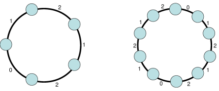
Figure 1: Example of two situations that are algorithmically indistinguishable. The numbers next to each edge are the edge labels.

Initially, the state $S_{i}(t)=[{x_{i}},y_{i}(t),z_{i}(t),m_{i,1}(t),m_{i,2}(t)]$, with $t=0$, of node $i$ in the first ring is exactly the same as the state of the nodes $j=i,i+n,i+2n,\ldots$ in the second ring. We show by induction that this property must hold at all times $t$. (To keep notation simple, we assume, without any real loss of generality, that $i\neq 1$ and $i\neq{n}$.)

Indeed, suppose this property holds up to time $t$. At time $t$, node $i$ in the first ring receives a message from node $i-1$ and a message from node $i+1$; and in the second ring, node $j$ satisfying ${j\ (\mbox{mod }n)}=i$ receives one message from $j-1$ and $j+1$. Since ${j-1\ (\mbox{mod }n)}=i-1{\ (\mbox{mod }n)}$ and ${j+1\ (\mbox{mod }n)}=i+1{\ (\mbox{mod }n)}$, the states of $j-1$ and $i-1$ are identical at time $t$, and similarly for $j+1$ and $i+1$. Thus, because of periodicity of the edge labels, nodes $i$ (in the first ring) and $j$ (in the second ring) receive identical messages through identically labeled ports at time $t$. Since $i$ and $j$ were in the same state at time $t$, they must be in the same state at time $t+1$. This proves that they are always in the same state. It follows that $y_{i}(t)=y_{j}(t)$ for all $t$, whenever ${j\ (\mbox{mod }n)}=i$, and therefore $f_{n}(x)=f_{mn}(x^{m})$. ∎

Proof of Theorem 3.1.

Let $x$ and $y$ be two sequences of $n$ and $m$ elements, respectively, such that $p_{k}(x_{1},\dots,x_{n})$ and $p_{k}(y_{1},\dots,y_{m})$ are equal to a common value $\hat{p}_{k}$, for ${k\in X}$; thus, the number of occurrences of $k$ in $x$ and $y$ are $n\hat{p}_{k}$ and $m\hat{p}_{k}$, respectively. Observe that for any $k\in X$, the vectors $x^{m}$ and $y^{n}$ have the same number $mn$ of elements, and both contain $mn\hat{p}_{k}$ occurrences of $k$. The sequences $y^{n}$ and $x^{m}$ can thus be obtained from each other by a permutation, which by Lemma 3.2 implies that $f_{nm}(x^{m})=f_{nm}(y^{n})$. From Lemma 3.3, we have that $f_{nm}(x^{m})=f_{n}(x)$ and $f_{mn}(y^{n})=f_{m}(y)$. Therefore, $f_{n}(x)=f_{m}(y)$. This proves that the value of $f_{n}(x)$ is determined by the values of $p_{k}(x_{1},\ldots,x_{n}),k=0,1,\ldots,K$. ∎

Remark: Observe that the above proof remains valid even under the “symmetry” assumption that an edge is assigned the same label by both of the nodes that it is incident on. port label of each edge is the same at every node.

4 Reduction of generic functions to the computation of averages

In this section, we turn to positive results, aiming at a converse of Theorem 3.1. The centerpiece of our development is Theorem 4.1, which states that a certain average-like function is computable. Theorem 4.1 then implies the computability of a large class of functions, yielding an approximate converse to Theorem 3.1. We will then illustrate these positive results on some examples.

The average-like functions that we consider correspond to the “interval consensus” problem studied in [7]. They are defined as follows. Let $X=\{0,\ldots,K\}$. Let $Y$ be the following set of single-point sets and intervals:

$$Y=\{\{0\},(0,1),\{1\},(1,2),\ldots,\{K-1\},(K-1,K),\{K\}\}$$

(or equivalently, an indexing of this finite collection of intervals). For any $n$, let $f_{n}$ be the function that maps $(x_{1},x_{2},\ldots,x_{n})$ to the element of $Y$ which contains the average $\sum_{i}x_{i}/n$. We refer to the function family $(f_{n})_{n=1,2,\ldots}$ as the interval-averaging family. The output of this family of functions is thus the exact average when it is an integer; otherwise, it is the open interval between two integers that contains the average.

The motivation for this function family comes from the fact that the exact average $\sum_{i}x_{i}/n$ takes values in a countably infinite set, and cannot be computed when the set $Y$ is finite. In the quantized averaging problem considered in the literature, one settles for an approximation of the average. However, such approximations do not necessarily define a single-valued function from $X^{n}$ into $Y$. In contrast, the above defined function $f_{n}$ is both single-valued and delivers an approximation with an error of size at most one. Note also that once the interval-average is computed, we can readily determine the value of the average rounded down to an integer.

Theorem 4.1.

The interval-averaging function family is computable.

The proof of Theorem 4.1 (and the corresponding algorithm) is quite involved; it will be developed in Sections 5 and 6. In this section, we show that the computation of a broad class of functions can be reduced to interval-averaging.

Since only frequency-based function families can be computable (Theorem 3.1), we can restrict attention to the corresponding functions $h$. We will say that a function $h$ on the unit simplex $D$ is computable if it corresponds to a frequency-based computable family $(f_{n})$. The level sets of $h$ are defined as the sets $L(y)=\{{p}\in D~{}|~{}h(p)=y\}$, for $y\in Y$.

Theorem 4.2 (Sufficient condition for computability).

Let $h$ be a function from the unit simplex $D$ to $Y$. Suppose that every level set $L(y)$ can be written as a finite union,

$$L(y)=\bigcup_{k}C_{i,k},$$

where each $C_{i,k}$ can in turn be written as a finite intersection of linear inequalities of the form

$${\alpha_{0}p_{0}}+\alpha_{1}p_{1}+\alpha_{2}p_{2}+\cdots+\alpha_{K}p_{K}\leq\alpha,$$ (4.1)

or

$${\alpha_{0}p_{0}}+\alpha_{1}p_{1}+\alpha_{2}p_{2}+\cdots+\alpha_{K}p_{K}<\alpha,$$

with rational coefficients $\alpha,{\alpha_{0}},\alpha_{1},\ldots,\alpha_{K}$. Then, $h$ is computable.

Proof.

Consider one such linear inequality, which we assume, for concreteness, to be of the form (4.1). Let $P$ be the set of indices $k$ for which $\alpha_{k}\geq 0$. Since all coefficients are rational, we can clear their denominators and rewrite the inequality as

$$\sum_{k\in P}\beta_{k}p_{k}-\sum_{{k}\in P^{c}}\beta_{k}p_{k}\leq\beta,$$ (4.2)

for nonnegative integers $\beta_{k}$ and $\beta$. Let $\chi_{k}$ be the indicator function associated with initial value $k$, i.e., $\chi_{k}(i)=1$ if $x_{i}=k$, and $\chi_{k}(i)=0$ otherwise, so that $p_{k}=\frac{1}{n}\sum_{i}\chi_{k}(i)$. Then, (4.2) becomes

$$\frac{1}{n}\sum_{i=1}^{n}\left(\sum_{k\in P}\beta_{k}\chi_{k}(i)+\sum_{k\in P^{c}}\beta_{k}(1-\chi_{k}(i))\right)\leq\beta+\sum_{k\in{P^{c}}}\beta_{k},$$

or

$$\frac{1}{n}\sum_{i{=1}}^{{n}}q_{i}\leq q^{*},$$

where $q_{i}=\sum_{k\in P}\beta_{k}\chi_{k}(i)+\sum_{k\in P^{c}}\beta_{k}(1-\chi_{k}(i))$ and $q^{*}=\beta+\sum_{k\in P^{c}}\beta_{k}$.

An algorithm that determines whether the last inequality is satisfied can be designed as follows. Knowing the parameters $\beta_{k}$ and the set $P$, which can be made part of algorithm description as they depend on the problem and not on the data, each node can initially compute its value $q_{i}$, as well as the value of $q^{*}$. Nodes can then apply the distributed algorithm that computes the integer part of $\frac{1}{n}\sum_{i=1}^{n}q_{i}$; this is possible by virtue of Theorem 4.1, with $K$ set to $\sum_{k}\beta_{k}$ (the largest possible value of $q_{i}$). It suffices then for them to constantly compare the current output of this algorithm to the integer $q^{*}$. To check any finite collection of inequalities, the nodes can perform the computations for each inequality in parallel.

To compute $h$, the nodes simply need to check which set $L(y)$ the frequencies ${p_{0}},p_{1},\ldots,p_{K}$ lie in, and this can be done by checking the inequalities defining each $L(y)$. All of these computations can be accomplished with finite automata: indeed, we do nothing more than run finitely many copies of the automata provided by Theorem 4.1, one for each inequality. The total memory used by the automata depends on the number of sets $C_{i,k}$ and the magnitude of the coefficients $\beta_{k}$, but not on $n$, as required. ∎

Theorem 4.2 shows the computability of functions $h$ whose level-sets can be defined by linear inequalities with rational coefficients. On the other hand, it is clear that not every function $h$ can be computable. (This can be shown by a counting argument: there are uncountably many possible functions $h$ on the rational elements of $D$, but for the special case of bounded degree graphs, only countably many possible algorithms.) Still, the next result shows that the set of computable functions is rich enough, in the sense that computable functions can approximate any measurable function, everywhere except possibly on a low-volume set.

We will call a set of the form $\prod_{{k}={0}}^{K}(a_{k},b_{k})$, with every $a_{k},b_{k}$ rational, a rational open box, where $\prod$ stands for Cartesian product. A function that can be written as a finite sum $\sum_{i}a_{i}{1_{B_{i}}}$, where the $B_{i}$ are rational open boxes and the $1_{B_{i}}$ are the associated indicator functions, will be referred to as a box function. Note that box functions are computable by Theorem 4.2.

Corollary 4.3.

If every level set of a function $h:D\to Y$ on the unit simplex $D$ is Lebesgue measurable, then, for every $\epsilon>0$, there exists a computable box function $h_{\epsilon}:D\to Y$ such that the set $\{p\in D~{}|~{}h(p)\neq h_{\epsilon}(p)\}$ has measure at most $\epsilon$.

Proof.

(Outline) The proof relies on the following elementary result from measure theory. Given a Lebesgue measurable set $E{\subseteq D}$ and some $\epsilon>0$, there exists a set $E^{\prime}$ which is a finite union of disjoint open boxes, and which satisfies

$$\mu({E\Delta E^{\prime}})<\epsilon,$$

where $\mu$ is the Lebesgue measure and $\Delta$ is the symmetric difference operator. By a routine argument, these boxes can be taken to be rational. By applying this fact to the level sets of the function $h$ (assumed measurable), the function $h$ can be approximated by a box function $h_{\epsilon}$. Since box functions are computable, the result follows. ∎

The following corollary states that continuous functions are approximable.

Corollary 4.4.

If a function $h:D\to[L,U]\subseteq\Re$ is continuous, then for every $\epsilon>0$ there exists a computable function $h_{\epsilon}:D{\to[L,U]}$ such that $\|h-h_{\epsilon}\|_{\infty}<\epsilon$

Proof.

Since $D$ is compact, $h$ is uniformly continuous. One can therefore partition $D$ into a finite number of subsets, $A_{1},A_{2},\dots,A_{q}$, that can be described by linear inequalities with rational coefficients, so that $\max_{p\in A_{j}}h(p)-\min_{p\in A_{j}}h(p)<\epsilon$ holds for all $A_{j}$. The function $h_{\epsilon}$ is then built by assigning to each $A_{j}$ an appropriate value in $\{L,L+\epsilon,L+2\epsilon,\dots,U\}$. ∎

To illustrate these results, let us consider again some examples.

(a)  Majority voting between two options is equivalent to checking whether $p_{1}\leq 1/2$, with alphabet $\{0,1\}$. This condition is clearly of the form (4.1), and is therefore computable.

(b)  Majority voting when some nodes can “abstain” amounts to checking whether $p_{1}-p_{{0}}\geq 0$, with input set ${X=}\{0,1,{\rm abstain}\}$. This function family is computable.

(c)  We can ask for the second most popular value out of four, for example. In this case, the sets $A_{i}$ can be decomposed into constituent sets defined by inequalities such as $p_{2}\leq p_{3}\leq p_{4}\leq p_{1}$, each of which obviously has rational coefficients. The level sets of the function can thus clearly be expressed as unions of sets defined by a collection of linear inequalities of the type (4.1), so that the function is computable.

(d)  For any subsets $I,I^{\prime}$ of $\{{0},1,\ldots,K\}$, the indicator function of the set where $\sum_{i\in I}p_{i}{>}\sum_{i\in I^{\prime}}p_{i}$ is computable. This is equivalent to checking whether more nodes have a value in $I$ than do in $I^{\prime}$.

(e)  The indicator functions of the sets defined by $p_{1}^{2}\leq 1/2$ and $p_{1}\leq\pi/4$ are measurable, so they are approximable. We are unable to say whether they are computable.

(f)  The indicator function of the set defined by $p_{1}p_{2}\leq 1/8$ is approximable, but we are unable to say whether it is computable.

Finally, we show that with infinite memory, it is possible to recover the exact frequencies $p_{k}$. (Note that this is impossible with finite memory, because $n$ is unbounded, and the number of bits needed to represent $p_{k}$ is also unbounded.) The main difficulty is that $p_{k}$ is a rational number whose denominator can be arbitrarily large, depending on the unknown value of $n$. The idea is to run separate algorithms for each possible value of the denominator (which is possible with infinite memory), and reconcile their results.

Theorem 4.5.

The vector $({p_{0}},p_{1},\ldots,p_{K})$ is computable with infinite memory.

Proof.

We show that $p_{1}$ is computable exactly, which is sufficient to prove the theorem. Consider the following algorithm, to be referred to as $Q_{m}$, parametrized by a positive integer $m$. The input set $X_{m}$ is $\{0,1,\ldots,m\}$ and the output set $Y_{m}$ is the same as in the interval-averaging problem: $Y_{m}=\{\{0\},(0,1),\{1\},(1,2),\{2\},(2,3),\ldots,\{m-1\},(m-1,m),\{m\}\}$. If $x_{i}=1$, then node sets its initial value $x_{i,m}$ to $m$; else, the node sets its initial value $x_{i,m}$ to $0$. The algorithm computes the function family $(f_{n})$ which maps $X_{m}^{n}$ to the element of $Y_{m}$ containing $(1/n)\sum_{i=1}^{n}x_{i,m}$, which is possible, by Theorem 4.1.

The nodes run the algorithms $Q_{m}$ for every positive integer value of $m$, in an interleaved manner. Namely, at each time step, a node runs one step of a particular algorithm $Q_{m}$, according to the following order:

$$Q_{1},\hskip 5.69046ptQ_{1},Q_{2},\hskip 5.69046ptQ_{1},Q_{2},Q_{3},\hskip 5.69046ptQ_{1},Q_{2},Q_{3},Q_{4},\hskip 5.69046ptQ_{1},Q_{2},\ldots$$

At each time $t$, let $m_{i}(t)$ be the smallest $m$ (if it exists) such that the output $y_{i,m}(t)$ of $Q_{m}$ at node $i$ is a singleton (not an interval). We identify this singleton with the numerical value of its single element, and we set $y_{i}(t)=y_{i,m_{i}(t)}(t)/m_{i}(t)$. If $m_{i}(t)$ is undefined, then $y_{i}(t)$ is set to some default value, e.g., $\emptyset$.

Let us fix a value of $n$. For any $m\leq n$, the definition of $Q_{m}$ and Theorem 4.1 imply that there exists a time after which the outputs ${y_{i,m}}$ of $Q_{m}$ do not change, and are equal to a common value, denoted $y_{m}$, for every $i$. Moreover, at least one of the algorithms $Q_{1},\ldots,Q_{n}$ has an integer output $y_{m}$. Indeed, observe that $Q_{n}$ computes $(1/n)\sum_{i=1}^{n}n1_{x_{i}=1}=\sum_{i=1}^{n}1_{x_{i}=1}$, which is clearly an integer. In particular, $m_{i}(t)$ is eventually well-defined and bounded above by $n$. We conclude that there exists a time after which the output $y_{i}(t)$ of our overall algorithm is fixed, shared by all nodes, and different from the default value $\emptyset$.

We now argue that this value is indeed $p_{1}$. Let $m^{*}$ be the smallest $m$ for which the eventual output of $Q_{m}$ is a single integer $y_{m}$. Note that $y_{m^{*}}$ is the exact average of the $x_{i,m^{*}}$, i.e.,

$$y_{m^{*}}=\frac{1}{n}\sum_{i=1}^{n}m^{*}1_{x_{i}=1}=m^{*}p_{1}.$$

For large $t$, we have $m_{i}(t)=m^{*}$ and therefore $y_{i}(t)=y_{i,m^{*}}(t)/m^{*}=p_{1}$, as desired.

Finally, it remains to argue that the algorithm described here can be implemented with a sequence of infinite memory automata. All the above algorithm does is run a copy of all the automata implementing $Q_{1},Q_{2},\ldots$ with time-dependent transitions. This can be accomplished with an automaton whose state space is the countable set $\mathcal{N}\times{\cup_{m=1}^{\infty}\prod_{i=1}^{m}{\cal Q}_{i}}$, where ${\cal Q}_{i}$ is the state space of $Q_{i}$, and the set $\mathcal{N}$ of integers is used to keep track of time. ∎

5 Computing and tracking maximal values

We now describe an algorithm that tracks the maximum (over all nodes) of time-varying inputs at each node. It will be used as a subroutine of the interval-averaging algorithm described in Section 6, and which is used to prove Theorem 4.1. The basic idea is the same as for the simple algorithm for the detection problem given in Section 2: every node keeps track of the largest value it has heard so far, and forwards this “intermediate result” to its neighbors. However, when an input value changes, the existing intermediate results need to be invalidated, and this is done by sending “restart” messages. A complication arises because invalidated intermediate results might keep circulating in the network, always one step ahead of the restart messages. We deal with this difficulty by “slowing down” the intermediate results, so that they travel at half the speed of the restart messages. In this manner, restart messages are guaranteed to eventually catch up with and remove invalidated intermediate results.

We start by giving the specifications of the algorithm. Suppose that each node $i$ has a time-varying input $u_{i}(t)$ stored in memory at time $t$, belonging to a finite set of numbers ${\cal U}$. We assume that, for each $i$, the sequence $u_{i}(t)$ must eventually stop changing, i.e., that there exists some $T^{\prime}$ such that

$$u_{i}(t)=u_{i}(T^{\prime}),~{}~{}~{}~{}~{}~{}~{}~{}\mbox{ for all }{i\mbox{ and }}t\geq T^{\prime}.$$

(However, node $i$ need not ever be aware that $u_{i}(t)$ has reached its final value.) Our goal is to develop a distributed algorithm whose output eventually settles on the value $\max_{i}u_{i}(T^{\prime})$. More precisely, each node $i$ is to maintain a number $M_{i}(t)$ which must satisfy the following condition: for every network and any allowed sequences $u_{i}(t)$, there exists some $T^{\prime\prime}$ with

$$M_{i}(t)=\max_{{j}=1,\ldots,n}u_{j}(t),~{}~{}~{}~{}~{}\mbox{ for all }{i\mbox{ and }}t\geq T^{\prime\prime}.$$

Moreover, each node $i$ must also maintain a pointer $P_{i}(t)$ to a neighbor or to itself. We will use the notation $P^{2}_{i}(t)=P_{P_{i}(t)}(t)$, $P^{3}_{i}(t)=P_{P_{i}^{2}(t)}(t)$, etc. We require the following additional property, for all $t$ larger than $T^{\prime\prime}$: for each node $i$ there exists a node ${j}$ and a power $K$ such that for all $k\geq K$ we have $P^{k}_{i}{(t)}=j$ and $M_{i}(t)=u_{j}(t)$. In words, by successively following the pointers $P_{i}(t)$, one can arrive at a node with a maximal value.

We next describe the algorithm. We will use the term slot $t$ to refer, loosely speaking, to the interval between times $t$ and $t+1$. More precisely, during slot $t$ each node processes the messages that have arrived at time $t$ and computes the state at time $t+1$ as well as the messages it will send at time $t+1$.

The variables $M_{i}(t)$ and $P_{i}(t)$ are a complete description of the state of node $i$ at time $t$. Our algorithm has only two types of messages that a node can send to its neighbors. Both are broadcasts, in the sense that the node sends them to every neighbor:

1. “Restart!”

2. “My estimate of the maximum is $y$,” where $y$ is some number in ${\cal U}$ chosen by the node.

Initially, each node sets $M_{i}(0)=u_{i}(0)$ and $P_{i}(0)=i$. At time $t=0,1,\ldots$, nodes exchange messages, which then determine their state at time $t+1$, i.e., the pair $M_{i}(t+1),P_{i}(t+1)$, as well as the messages to be sent at time $t+1$. The procedure node $i$ uses to do this is described in Figure 2. One can verify that a memory size of $C\log|{\cal U}|+C\log d(i)$ at each node $i$ suffices, where $C$ is an absolute constant. (This is because $M_{i}$ and $P_{i}$ can take one of $|{\cal U}|$ and $d(i)$ possible values, respectively.)

The result that follows asserts the correctness of the algorithm. The idea of the proof is quite simple. Nodes maintain estimates $M_{i}(t)$ which track the largest among all the $u_{i}(t)$ in the graph; these estimates are “slowly” forwarded by the nodes to their neighbors, with many artificial delays along the way. Should some value $u_{j}(t)$ change, restart messages traveling without artificial delays are forwarded to any node which thought $j$ had a maximal value, causing those nodes to start over. The possibility of cycling between restarts and forwards is avoided because restarts travel faster. Eventually, the variables $u_{i}(t)$ stop changing, and the algorithm settles on the correct answer. On the other hand a formal and rigorous exposition of this simple argument is rather tedious. A formal proof is available in Appendix A.

Theorem 5.1 (Correctness of the maximum tracking algorithm).

Suppose that the $u_{i}(t)$ stop changing after some finite time. Then, for every network, there is a time after which the variables $P_{i}(t)$ and $M_{i}(t)$ stop changing and satisfy $M_{i}(t)=\max_{i}u_{i}(t)$; furthermore, after that time, and for every $i$, the node $j=P_{i}^{n}(t)$ satisfies $M_{i}(t)=u_{j}(t)$.

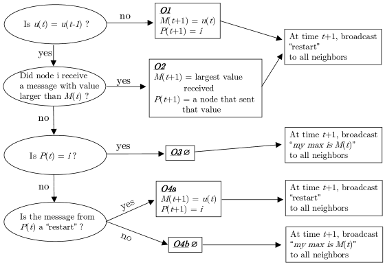
Figure 2: Flowchart of the procedure used by node $i$ during slot $t$ in the maximum tracking algorithm. The subscript $i$ is omitted, but $u(t)$, $M(t)$, and $P(t)$ should be understood as $u_{i}(t)$, $M_{i}(t)$, and $P_{i}(t)$. In those cases where an updated value of $M$ or $P$ is not indicated, it is assumed that $M(t+1)=M(t)$ and $P(t+1)=P(t)$. The symbol $\emptyset$ is used to indicate no action. Note that the various actions indicated are taken during slot $t$, but the messages determined by these actions are sent (and instantaneously received) at time $t+1$. Finally, observe that every node sends an identical message to all its neighbors at every time $t>0$. We note that the apparent non-determinism in instruction O2 can be removed by picking a node with, say, the smallest port label.

6 Interval-averaging

In this section, we present an interval-averaging algorithm and prove its correctness. We start with an informal discussion of the main idea. Imagine the integer input value $x_{i}$ as represented by a number of $x_{i}$ pebbles at node $i$. The algorithm attempts to exchange pebbles between nodes with unequal numbers so that the overall distribution becomes more even. Eventually, either all nodes will have the same number of pebbles, or some will have a certain number and others just one more. We let $u_{i}(t)$ be the current number of pebbles at node $i$; in particular, $u_{i}(0)=x_{i}$. An important property of the algorithm will be that the total number of pebbles is conserved.

To match nodes with unequal number of pebbles, we use the maximum tracking algorithm of Section 5. Recall that the algorithm provides nodes with pointers which attempt to track the location of the maximal values. When a node with ${u}_{i}$ pebbles comes to believe in this way that a node with at least $u_{i}+2$ pebbles exists, it sends a request in the direction of the latter node to obtain one or more pebbles. This request follows a path to a node with a maximal number of pebbles until the request either gets denied, or gets accepted by a node with at least $u_{i}+2$ pebbles.

6.1 The algorithm

The algorithm uses two types of messages. Each type of message can be either originated at a node or forwarded by a node.

(a)  (Request, $r$): This is a request for a transfer of pebbles. Here, $r$ is an integer that represents the number of pebbles $u_{i}(t)$ at the node $i$ that first originated the request, at the time $t$ that the request was originated. (Note, however, that this request is actually sent at time $t+1$.)

(b)  (Accept, $w$): This corresponds to acceptance of a request, and a transfer of $w$ pebbles towards the node that originated the request. An acceptance with a value $w=0$ represents a request denial.

As part of the algorithm, the nodes run the maximum tracking algorithm of Section 5, as well as a minimum tracking counterpart. In particular, each node $i$ has access to the variables $M_{i}(t)$ and $P_{i}(t)$ of the maximum tracking algorithm (recall that these are, respectively, the estimated maximum and a pointer to a neighbor or to itself). Furthermore, each node maintains three additional variables.

(a)  “Mode($t$)”$\in$ {Free, Blocked}. Initially, the mode of every node is free. A node is blocked if it has originated or forwarded a request, and is still waiting to hear whether the request is accepted (or denied).

(b)  “$\mbox{Rin}_{i}(t)$” and “$\mbox{Rout}_{i}(t)$” are pointers to a neighbor of $i$, or to $i$ itself. The meaning of these pointers when in blocked mode are as follows. If $\mbox{Rout}_{i}(t)=j$, then node $i$ has sent (either originated or forwarded) a request to node $j$, and is still in blocked mode, waiting to hear whether the request is acceptd or denied. If $\mbox{Rin}_{i}(t)=k$, and $k\neq i$, then node $i$ has received a request from node $k$ but has not yet responded to node $k$. If $\mbox{Rin}_{i}(t)=i$, then node $i$ has originated a request and is still in blocked mode, waiting to hear whether the request is accepted or denied.

A precise description of the algorithm is given in Figure 3. The proof of correctness is given in the next subsection, thus also establishing Theorem 4.1. Furthermore, we will show that the time until the algorithm settles on the correct output is of order $O(n^{2}K^{2})$.

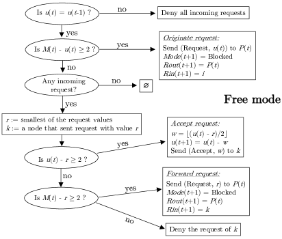
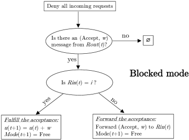
Figure 3: Flowchart of the procedure used by node $i$ during slot $t$ in the interval-averaging algorithm. The subscript $i$ is omitted from variables such as Mode$(t)$, $M(t)$, etc. Variables for which an update is not explicitly indicated are assumed to remain unchanged. “Denying a request” is a shorthand for $i$ sending a message of the form (Accept, 0) at time $t+1$ to a node from which $i$ received a request at time $t$. Note also that “forward the acceptance” in the blocked mode includes the case where the answer had $w=0$ (i.e., it was a request denial), in which case the denial is forwarded.

6.2 Proof of correctness

We begin by arguing that that the rules of the algorithm preclude one potential obstacle; we will show that nodes will not get stuck sending requests to themselves.

Lemma 6.1.

A node never sends (originates or forwards) a request to itself. More precisely, $\mbox{Rout}_{i}(t)\neq i$, for all $i$ and $t$.

Proof.

By inspecting the first two cases for the free mode, we observe that if node $i$ originates a request during time slot $t$ (and sends a request message at time $t+1$), then $P_{i}(t)\neq i$. Indeed, to send a message, it must be true $M_{i}(t)>u_{i}(t)=u_{i}(t-1)$. However, any action of the maximum tracking algorithm that sets $P_{i}(t)=i$ also sets $M_{i}(t)=u_{i}(t-1)$, and moreover, as long as $P_{i}$ doesn’t change neither does $M_{i}$. So the recipient $P_{i}(t)$ of the request originated by $i$ is different than $i$, and accordingly, $\mbox{Rout}_{i}{(t+1)}$ is set to a value different than $i$. We argue that the same is true for the case where $\mbox{Rout}_{i}$ is set by the the “Forward request” box of the free mode. Indeed, that box is enabled only when $u_{i}(t)=u_{i}(t-1)$ and $u_{i}(t)-1\leq r<M_{i}(t)-1$, so that $u_{i}(t-1)<M_{i}(t)$. As in the previous case, this implies that $P_{i}(t)\neq i$ and that $\mbox{Rout}_{i}(t+1)$ is again set to a value other than $i$. We conclude that $\mbox{Rout}_{i}(t)\neq i$ for all $i$ and $t$. ∎

We will now analyze the evolution of the requests. A request is originated at some time $\tau$ by some originator node $\ell$ who sets $\mbox{Rin}_{\ell}(\tau+1)=\ell$ and sends the request to some node $i=\mbox{Rout}_{\ell}(\tau+1)=P_{\ell}(\tau)$. The recipient $i$ of the request either accepts/denies it, in which case $\mbox{Rin}_{i}$ remains unchanged, or forwards it while also setting $\mbox{Rin}_{i}(\tau+2)$ to $\ell$. The process then continues similarly. The end result is that at any given time $t$, a request initiated by node $\ell$ has resulted in a “request path of node $\ell$ at time $t$,” which is a maximal sequence of nodes $\ell,i_{1},\ldots,i_{k}$ with $\mbox{Rin}_{\ell}(t)=\ell$, $\mbox{Rin}_{i_{1}}(t)=\ell$, and $\mbox{Rin}_{i_{m}}(t)=i_{m-1}$ for $m\leq k$.

Lemma 6.2.

At any given time, different request paths cannot intersect (they involve disjoint sets of nodes). Furthermore, at any given time, a request path cannot visit the same node more than once.

Proof.

For any time $t$, we form a graph that consists of all edges that lie on some request path. Once a node $i$ is added to some request path, and as long as that request path includes $i$, node $i$ remains in blocked mode and the value of $\mbox{Rin}_{i}$ cannot change. This means that adding a new edge that points into $i$ is impossible. This readily implies that cycles cannot be formed and also that two request paths cannot involve a common node. ∎

We use $p_{\ell}(t)$ to denote the request path of node $\ell$ at time $t$, and $s_{\ell}(t)$ to denote the last node on this path. We will say that a request originated by node $\ell$ terminates when node $\ell$ receives an (Accept, $w$) message, with any value $w$.

Lemma 6.3.

Every request eventually terminates. Specifically, if node $\ell$ originates a request at time $t^{\prime}$ (and sends a request message at time $t^{\prime}+1$), then there exists a later time $t^{\prime\prime}\leq t^{\prime}+n$ at which node $s_{r}(t^{\prime\prime})$ receives an “accept request” message (perhaps with $w=0$), which is forwarded until it reaches $\ell$, no later than time $t^{\prime\prime}+n$.

Proof.

By the rules of our algorithm, node $\ell$ sends a request message to node $P_{\ell}(t^{\prime})$ at time $t^{\prime}+1$. If node $P_{\ell}(t^{\prime})$ replies at time $t^{\prime}+2$ with a “deny request” response to $\ell$’s request, then the claim is true; otherwise, observe that $p_{\ell}(t^{\prime}+{2})$ is nonempty and until $s_{\ell}(t)$ receives an “accept request” message, the length of $p_{\ell}(t)$ increases at each time step. Since this length cannot be larger than $n{-1}$, by Lemma 6.2, it follows that $s_{\ell}(t)$ receives an “accept request” message at most $n$ steps after $\ell$ initiated the request. One can then easily show that this acceptance message is forwarded backwards along the path (and the request path keeps shrinking) until the acceptance message reaches $\ell$, at most $n$ steps later. ∎

The arguments so far had mostly to do with deadlock avoidance. The next lemma concerns the progress made by the algorithm. Recall that a central idea of the algorithm is to conserve the total number of “pebbles,” but this must include both pebbles possessed by nodes and pebbles in transit. We capture the idea of “pebbles in transit” by defining a new variable. If $i$ is the originator of some request path that is present at time $t$, and if the final node $s_{i}(t)$ of that path receives an (Accept, $w$) message at time $t$, we let $w_{i}(t)$ be the value $w$ in that message. (This convention includes the special case where $w=0$, corresponding to a denial of the request). In all other cases, we set $w_{i}(t)=0$. Intuitively, $w_{i}(t)$ is the value that has already been given away by a node who answered a request originated by node $i$, and that will eventually be added to $u_{i}$, once the answer reaches $i$.

We now define

$$\hat{u}_{i}(t)=u_{i}(t)+w_{i}(t).$$

By the rules of our algorithm, if $w_{i}(t){=w}>0$, an amount $w$ will eventually be added to $u_{i}$, once the acceptance message is forwarded back to $i$. The value $\hat{u}_{i}$ can thus be seen as a future value of $u_{i}$, that includes its present value and the value that has been sent to $i$ but has not yet reached it.

The rules of our algorithm imply that the sum of the $\hat{u}_{i}$ remain constant. Let $\bar{x}$ be the average of the initial values $x_{i}$. Then,

$$\frac{1}{n}\sum_{i=1}^{n}\hat{u}_{i}(t)=\frac{1}{n}\sum_{i=1}^{n}x_{i}=\bar{x}.$$

We define the variance function $V$ as

$$V(t)=\sum_{i=1}^{n}(\hat{u}_{i}(t)-\bar{x})^{2}.$$

Lemma 6.4.

The number of times that a node can send an acceptance message (Accept, $w$) with $w\neq 0$, is finite.

Proof.

Let us first describe the idea behind the proof. Suppose that nodes could instantaneously transfer value to each other. It is easily checked that if a node $i$ transfers an amount $w^{*}$ to a node $j$ with $u_{i}-u_{j}\geq 2$ and $1\leq w^{*}\leq\frac{1}{2}(u_{i}-u_{j})$, the variance $\sum_{i}(u_{i}-{\bar{x}})^{2}$ decreases by at least 2. Thus, there can only be a finite number of such transfers. In our model, the situation is more complicated because transfers are not immediate and involve a process of requests and acceptances. A key element of the argument is to realize that the algorithm can be interpreted as if it only involved instantaneous exchanges involving disjoint pairs of nodes.

Let us consider the difference $V(t+1)-V(t)$ at some typical time $t$. Changes in $V$ are solely due to changes in the $\hat{u}_{i}$. Note that if a node $i$ executes the “fulfill the acceptance” instruction at time $t$, node $i$ was the originator of the request and the request path has length zero, so that it is also the final node on the path, and $s_{i}(t)=i$. According to our definition, $w_{i}(t)$ is the value $w$ in the message received by node $s_{i}(t)=i$. At the next time step, we have $w_{i}(t+1)=0$ but $u_{i}(t+1)=u_{i}(t)+w$. Thus, $\hat{u}_{i}$ does not change, and the function $V$ is unaffected.

By inspecting the algorithm, we see that a nonzero difference $V(t+1)-V(t)$ is possible only if some node $i$ executes the “accept request” instruction at slot $t$, with some particular value $w^{*}{\neq 0}$, in which case $u_{i}(t+1)=u_{i}(t)-w^{*}$. For this to happen, node $i$ received a message (Request, $r$) at time $t$ from a node $k$ for which $\mbox{Rout}_{k}(t)=i$, and with $u_{i}(t)-r\geq 2$. That node $k$ was the last node, $s_{\ell}(t)$, on the request path of some originator node $\ell$. Node $k$ receives an (Accept, $w^{*}$) message at time $t+1$ and, therefore, according to our definition, this sets $w_{\ell}(t+1)=w^{*}$.

It follows from the rules of our algorithm that $\ell$ had originated a request with value $r=u_{\ell}(t^{\prime})$ at some previous time $t^{\prime}$. Subsequently, node $\ell$ entered the blocked mode, preventing any modification of $u_{\ell}$, so that $r=u_{\ell}(t)=u_{\ell}(t+1)$. Moreover, observe that $w_{\ell}(t)$ was 0 because by time $t$, no node had answered $\ell$’s request. Furthermore, $w_{i}(t+1)=w_{i}(t)=0$ because having a positive $w_{i}$ requires $i$ to be in blocked mode, preventing the execution of “accept request”. It follows that

$$\hat{u}_{i}(t+1)=u_{i}(t+1)=u_{i}(t)-w^{*}=\hat{u}_{i}(t)-w^{*},$$

and

$$\hat{u}_{\ell}(t+1)=r+w^{*}=\hat{u}_{\ell}(t)+w^{*}.$$

Using the update equation $w^{*}=\lfloor(u_{i}(t)-r)/2\rfloor$, and the fact $u_{i}(t)-r\geq 2$, we obtain

$$1\leq w^{*}\leq\frac{1}{2}(u_{i}(t)-r)=\frac{1}{2}(\hat{u}_{i}(t)-\hat{u}_{\ell}(t)).$$

Combining with the previous equalities, we have

$$\hat{u}_{\ell}(t)+1\leq\hat{u}_{\ell}(t+1)\leq\hat{u}_{i}(t+1)\leq\hat{u}_{i}(t)-1.$$

Assume for a moment that node $i$ was the only one that executed the “accept request” instruction at time $t$. Then, all of the variables $\hat{u}_{j}$, for $j\neq i,\ell$, remain unchanged. Simple algebraic manipulations then show that $V$ decreases by at least 2. If there was another pair of nodes, say $j$ and $k$, that were involved in a transfer of value at time $t$, it is not hard to see that the transfer of value was related to a different request, involving a separate request path. In particular, the pairs $\ell,i$ and $j,k$ do not overlap. This implies that the cumulative effect of multiple transfers on the difference $V(t+1)-V(t)$ is the sum of the effects of individual transfers. Thus, at every time for which at least one “accept request” step is executed, $V$ decreases by at least 2. We also see that no operation can ever result in an increase of $V$. It follows that the instruction “accept request” can be executed only a finite number of times. ∎

Proposition 6.1.

There is a time $t^{\prime}$ such that $u_{i}(t)=u_{i}(t^{\prime})$, for all $i$ and all $t\geq t^{\prime}$. Moreover,

$$\sum_{i}u_{i}(t^{\prime}) = \sum_{i}x_{i},$$

$${\max_{i}u_{i}(t^{\prime})-\min_{i}u_{i}(t^{\prime})} \leq 1.$$

Proof.

It follows from Lemma 6.4 that there is a time $t^{\prime}$after which no more requests are accepted with $w\neq 0$. By Lemma 6.3, this implies that after at most $n$ additional time steps, the system will never again contain any “accept request” messages with $w\neq 0$, so no node will change its value $u_{i}(t)$ thereafter.

We have already argued that the sum (and therefore the average) of the variables $\hat{u}_{i}(t)$ does not change. Once there are no more “accept request” messages in the system with $w\neq 0$, we must have $w_{i}(t)=0$, for all $i$. Thus, at this stage the average of the $u_{i}(t)$ is the same as the average of the $x_{i}$.

It remains to show that once the $u_{i}(t)$ stop changing, the maximum and minimum $u_{i}(t)$ differ by at most $1$. Recall (cf. Theorem that 5.1) that at some time after the $u_{i}(t)$ stop changing, all estimates $M_{i}(t)$ of the maximum will be equal to $M(t)$, the true maximum of the $u_{i}(t)$; moreover, starting at any node and following the pointers $P_{i}(t)$ leads to a node $j$ whose value $u_{j}(t)$ is the true maximum, $M(t)$. Now let $A$ be the set of nodes whose value at this stage is at most $\max_{i}u_{i}(t)-2$. To derive a contradiction, let us suppose that $A$ is nonempty.

Because only nodes in $A$ will originate requests, and because every request eventually terminates (cf. Lemma 6.3), if we wait some finite amount of time, we will have the additional property that all requests in the system originated from $A$. Moreover, nodes in $A$ originate requests every time they are in the free mode, which is infinitely often.

Consider now a request originating at a node in the set $A$. The value $r$ of such a request satisfies $M(t)-r\geq 2$, which implies that every node that receives it either accepts it (contradicting the fact that no more requests are accepted after time $t^{\prime}$), or forwards it, or denies it. But a node $i$ will deny a request only if it is in blocked mode, that is, if it has already forwarded some other request to node $P_{i}(t)$. This shows that requests will keep propagating along links of the form $(i,P_{i}(t))$, and therefore will eventually reach a node at which $u_{i}(t)=M(t)\geq r+2$, at which point they will be accepted—a contradiction. ∎

We are now ready to conclude.

Proof of Theorem 4.1.

Let $u_{i}^{*}$ be the value that $u_{i}(t)$ eventually settles on. Proposition 6.1 readily implies that if the average $\bar{x}$ of the $x_{i}$ is an integer, then $u_{i}(t)=u_{i}^{*}=\bar{x}$ will eventually hold for every $i$. If $\bar{x}$ is not an integer, then some nodes will eventually have $u_{i}(t)=u_{i}^{*}=\lfloor\bar{x}\rfloor$ and some other nodes $u_{i}(t)=u_{i}^{*}=\lceil\bar{x}\rceil$. Besides, using the maximum and minimum computation algorithm, nodes will eventually have a correct estimate of $\max u_{i}^{*}$ and $\min u_{i}^{*}$, since all $u_{i}(t)$ settle on the fixed values $u_{i}^{*}$. This allows the nodes to determine whether the average is exactly $u^{*}_{i}$ (integer average), or whether it lies in $(u_{i}^{*},u_{i}^{*}+1)$ or $(u_{i}^{*}-1,u^{*}_{i})$ (fractional average). Thus, with some simple post-processing at each node (which can be done using finite automata), the nodes can produce the correct output for the interval-averaging problem. The proof of Theorem 4.1 is complete. ∎

Next, we give a convergence time bound for the algorithms we have just described.

Theorem 6.1.

Any function $h$ satisfying the assumptions of Theorem 4.2 can be computed in $O(n^{2}K^{2})$ time steps.

Theorem 6.2.

The functions $h_{\epsilon}$ whose existence is guaranteed by Corollary 4.3 or Corollary 4.4 can be computed in time which grows quadratically in $n$.

The general idea behind Theorems 6.1 and 6.2 is quite simple. We have just argued that the nonnegative function $V(t)$ decreases by at least $2$ each time a request is accepted. It also satisfies $V(0)=O(nK^{2})$. Thus there are at most $O(nK^{2})$ acceptances. To prove Theorems 6.1 and 6.2 is, one needs to argue that if the algorithm has not terminated, there will be an acceptance within $O(n)$ time steps. This should be fairly clear from the proof of Theorem 4.1. A formal argument is given in Appendix B. It is also shown there that the running time of our algorithm, for many graphs, satisfies a $\Omega(n^{2})$ lower bound, in the worst case over all initial conditions.

7 Simulations

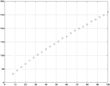
Figure 4: The number of iterations as a function of the number of nodes for a complete graph under random initial conditions.

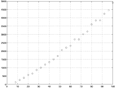
Figure 5: The number of iterations as a function of the number of nodes for a line graph under random initial conditions.

We report here on simulations involving our algorithm on several natural graphs. Figures 5 and 5 describe the results for a complete graph and a line. Initial conditions were random integers between $1$ and $30$, and each data point represents the average of two hundred runs. As expected, convergence is faster on the complete graph. Moreover, convergence time in both simulations appears to be approximately linear.

Finally recall that it is possible for our algorithm to take on the order of $n^{2}$ (as opposed to $O(n)$) time steps to converge. Figure 6 shows simulation results for the dumbbell graph (two complete graphs with $n/3$ nodes, connected by a line) of length $n/3$; each node in one of the complete graphs starts with $x_{i}(0)=1$, every node in the other complete graph starts with $x_{i}(0)=30$. The time to converge in this case is quadratic in $n$.

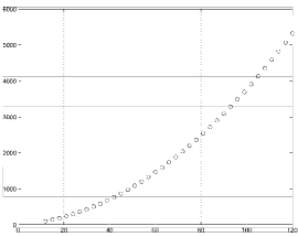
Figure 6: The number of iterations as a function of the number of nodes for a dumbbell graph.

8 Conclusions

We have proposed a model of deterministic anonymous distributed computation, inspired by the wireless sensor network and multi-agent control literature. We have given an almost tight characterization of the functions that are computable in our model. We have shown that computable functions must depend only on the the frequencies with which the different initial conditions appear, and that if this dependence can be expressed in term of linear inequalities with rational coefficients, the function is indeed computable. Under weaker conditions, the function can be approximated with arbitrary precision. It remains open to exactly characterize the class of computable function families.

Our positive results are proved constructively, by providing a generic algorithm for computing the desired functions. Interestingly, the finite memory requirement is not used in our negative results, which remain thus valid in the infinite memory case. In particular, we have no examples of functions that can be computed with infinite memory but are provably not computable with finite memory. We suspect though that simple examples exist; a good candidate could be the indicator function $1_{p_{1}<1/\pi}$, which checks whether the fraction of nodes with a particular initial condition is smaller than $1/\pi$.

We have shown that our generic algorithms terminate in $O(n^{2})$ time. On the other hand, it is clear that the termination time cannot be faster than the graph diameter, which is of order $n$, in the worst case. Some problems, such as the detection problem described in Section 2, admit $O(n)$ algorithms. On the other hand, it is an open problem whether the interval averaging problem admits an $o(n^{2})$ algorithm under our model. Finally, we conjecture that the dependence on $K$ in our $O(n^{2}K^{2})$ complexity estimate can be improved by designing a different algorithm.

Possible extensions of this work involve variations of the model of computation. For example, the algorithm for detection problem, described in Section 2, does not make full use of the flexibility allowed by our model of computation. In particular, for any given $i$, the messages $m_{ij}(t)$ are the same for all $j$, so, in some sense, messages are “broadcast” as opposed to being personalized for the different outgoing links. This raises an interesting question: do there exist computable function families that become non-computable when we restrict to algorithms that are limited to broadcast messages? We have reasons to believe that in a pure broadcast scenario where nodes located in a non-bidirectional network broadcast messages without knowing their out-degree (i.e., the size of their audience), the only computable functions are those which test whether there exists a node whose initial condition belongs to a given subset of $\{0,1,\ldots,K\}$, and combinations of such functions.

Another important direction is to consider models in which the underlying graph may vary with time. It is of interest to develop algorithms that converge to the correct answer at least when the underlying graph eventually stops changing. For the case where the graph keeps changing while maintaining some degree of connectivity, we conjecture that no deterministic algorithm with bounded memory can solve the interval-averaging problem. Finally, other extensions involve models accounting for clock asynchronism, delays in message propagation, or data loss.

Appendix A Proof of Theorem 5.1

In the following, we will occasionally use the following convenient shorthand: we will say that a statement $S(t)$ holds eventually if there exists some $T$ so that $S(t)$ is true for all $t\geq T$.

The analysis is made easier by introducing the time-varying directed graph $G(t)=(\{1,\ldots,n\},E(t))$ where $(i,j)\in E(t)$ if $i\neq j$, $P_{i}(t)=j$, and there is no “restart” message sent by $j$ (and therefore received by $i$) during time $t$. We will abuse notation by writing $(i,j)\in G(t)$ to mean that the edge $(i,j)$ belongs to the set of edges $E(t)$ at time $n$.

Lemma A.1.

Suppose that $(i,j)\notin G(t-1)$ and $(i,j)\in G(t)$. Then, $i$ executes O2 during slot $t-1$.

Proof.

Suppose that $(i,j)\notin G(t-1)$ and $(i,j)\in G(t)$. If $P_{i}(t-1)=j$, the definition of $G(t-1)$ implies that $j$ sent a restart message to $i$ at time $t-1$. Moreover, $i$ cannot execute O3 during the time slot $t-1$ as this would require $P_{i}(t-1)=i$.Therefore, during this time slot, node $i$ either executes O2 (and we are done) or it executes one of O1 and O4a. For both of the latter two cases, we will have $P_{i}(t)=i$, so that $(i,j)$ will not be in $G(t)$, a contradiction. Thus, it must be that $P_{i}(t-1)\neq j$. We now observe that the only place in Figure 2 that can change $P_{i}(t-1){\neq j}$ to $P_{i}(t)=j$ is O2. ∎

Lemma A.2.

In each of the following three cases, node $i$ has no incoming edges in either graph $G(t)$ or $G(t+1)$:
(a) Node $i$ executes O1, O2, or O4a during time slot $t-1$;
(b) $M_{i}(t)\not=M_{i}(t-1)$;
(c) For some $j$, $(i,j)\in G(t)$ but $(i,j)\notin G(t-1).$

Proof.

(a) If $i$ executes O1, O2, or O4a during slot $t-1$, then it sends a restart message to each of its neighbors at time $t$. Then, for any neighbor $j$ of $i$, the definition of $G(t)$ implies that $(j,i)$ is not in $G(t)$. Moreover, by Lemma A.1, in order for $(j,i)$ to be in $G(t+1)$, node $j$ must execute $O2$ during slot $t$. But the execution of O2 during slot $t$ cannot result in the addition of the edge $(j,i)$ at time $t+1$, because the message broadcast by $i$ at time $t$ to its neighbors was a restart. So, $(j,i)\notin G(t+1)$.

(b) If $M_{i}(t)\not=M_{i}(t-1)$, then $i$ executes O1, O2, or O4a during slot $t-1$, so the claim follows from part (a).

(c) By Lemma A.1, it must be the case that node $i$ executes O2 during slot $t-1$, and part (a) implies the result. ∎

Lemma A.3.

The graph $G(t)$ is acyclic, for all $t$.

Proof.

The initial graph $G(0)$ does not contain a cycle. Let $t$ be the first time a cycle is present, and let $(i,j)$ be an edge in a cycle that is added at time $t$, i.e., $(i,j)$ belongs to $G(t)$ but not $G(t-1)$. Lemma A.2(c) implies that $i$ has no incoming edges in $G(t)$, so $(i,j)$ cannot be an edge of the cycle—a contradiction. ∎

Note that every node has out-degree at most one, because $P_{i}(t)$ is a single-valued variable. Thus, the acyclic graph $G(t)$ must be a forest, specifically, a collection of disjoint trees, with all arcs of a tree directed so that they point towards a root of the tree (i.e., a node with zero out-degree). The next lemma establishes that $M_{i}$ is constant on any path of $G(t)$.

Lemma A.4.

If $(i,j)\in G(t)$, then $M_{i}(t)=M_{j}(t)$.

Proof.

Let $t^{\prime}$ be a time when $(i,j)$ is added to the graph, or more precisely, a time such that $(i,j)\in G(t^{\prime})$ but $(i,j)\notin G(t^{\prime}-1)$. First, we argue that the statement we want to prove holds at time $t^{\prime}$. Indeed, Lemma A.1 implies that during slot $t^{\prime}-1$, node $i$ executed $O2$, so that $M_{i}(t^{\prime})=M_{j}(t^{\prime}-1)$. Moreover, $M_{j}(t^{\prime}-1)=M_{j}(t^{\prime})$, because otherwise case (b) in Lemma A.2 would imply that $j$ has no incoming edges at time $t^{\prime}$, contradicting our assumption that $(i,j)\in G(t^{\prime})$.

Next, we argue that the property $M_{i}(t)=M_{j}(t)$ continues to hold, starting from time $t^{\prime}$ and for as long as $(i,j)\in G(t)$. Indeed, as long as $(i,j)\in G(t)$, then $M_{j}(t)$ remains unchanged, by case (b) of Lemma A.2. To argue that $M_{i}(t)$ also remains unchanged, we simply observe that in Figure 1, every box which leads to a change in $M_{i}$ also sets $P_{i}$ either to $i$ or to the sender of a message with value strictly larger than $M_{i}$; this latter message cannot come from $j$ because as we just argued, increases in $M_{j}$ lead to removal of the edge $(i,j)$ from $G(t)$. So, changes in $M_{i}$ are also accompanied by removal of the edge $(i,j)$ from $G(t)$. ∎

For the purposes of the next lemma, we use the convention $u_{i}(-1)=u_{i}(0)$.

Lemma A.5.

If $P_{i}(t)=i$, then $M_{i}(t)=u_{i}(t-1)$; if $P_{i}(t)\neq i$, then $M_{i}(t)>u_{i}(t{-}1)$.

Proof.

We prove this result by induction. Because of the convention $u_{i}(-1)=u_{i}(0)$, and the initialization $P_{i}(0)=i$, $M_{i}(0)=u_{i}(0)$, the result trivially holds at time $t=0$. Suppose now that the result holds at time $t$. During time slot $t$, we have three possibilities for node $i$:

• Node $i$ executes O1 or O4a. In this case, $M_{i}(t+1)=u_{i}(t),P_{i}(t+1)=i$, so the result holds at time $t+1$.

• Node $i$ executes O2. In this case $P_{i}(t)\neq i$ and $M_{i}(t+1)>M_{i}(t)\geq u_{i}(t-1)=u_{i}(t)$. The first inequality follows from the condition for entering step O2. The second follows from the induction hypothesis. The last equality follows because if $u_{i}(t)\neq u_{i}(t-1)$, node $i$ would have executed O1 rather than O2. So, once again, the result holds at time $t+1$.

• Node $i$ executes O3 or O4b. The result holds at time $t+1$ because neither $u_{i}$ nor $M_{i}$ changes.

∎

In the sequel, we will use $T^{\prime}$ to refer to a time after which all the $u_{i}$ are constant. The following lemma shows that, after $T^{\prime}$, the largest estimate does not increase.

Lemma A.6.

Suppose that at some time $t^{\prime}>T^{\prime}$ we have $\widehat{M}>\max_{i}M_{i}(t^{\prime})$. Then

$$\widehat{M}>\max_{i}M_{i}(t)$$ (A.3)

for all $t\geq t^{\prime}$.

Proof.

We prove Eq. (A.3) by induction. By assumption it holds at time $t=t^{\prime}$. Suppose now Eq. (A.3) holds at time $t$; we will show that it holds at time $t+1$.

Consider a node $i$. If it executes O2 during the slot $t$, it sets $M_{i}(t+1)$ to the value contained in a message sent at time $t$ by some node $j$. It follows from the rules of our algorithm that the value in this message is $M_{j}(t)$ and therefore, $M_{i}(t+1)=M_{j}(t)<\widehat{M}$.

Any operation other than O2 that modifies $M_{i}$ sets $M_{i}(t+1)=u_{i}(t)$, and since $u_{i}(t)$ does not change after time $T^{\prime}$, we have $M_{i}(t+1)=u_{i}(t-1)$. By Lemma A.5, $M_{i}(t)\geq u_{i}(t-1)$, so that $M_{i}(t+1)\leq M_{i}(t)$. We conclude that $M_{i}(t+1)<\widehat{M}$ holds for this case as well. ∎

We now introduce some terminology used to specify whether the estimate $M_{i}(t)$ held by a node has been invalidated or not. Formally, we say that node $i$ has a valid estimate at time $t$ if by following the path in $G(t)$ that starts at $i$, we eventually arrive at a node $r$ with $P_{r}(t)=r$ and $M_{i}(t)=u_{r}(t-1)$. In any other case, we say that a node has an invalid estimate at time $t$.

Remark: Because of the acyclicity property, a path in $G(t)$, starting from a node $i$, eventually leads to a node $r$ with out-degree 0; it follows from Lemma A.4 that $M_{r}(t)=M_{i}(t)$. Moreover, Lemma A.5 implies that if $P_{r}(t)=r$, then $M_{i}(t)=M_{r}(t)=u_{r}({t-1})$, so that the estimate is valid. Therefore, if $i$ has an invalid estimate, the corresponding node $r$ must have $P_{r}(t)\not=r$; on the other hand, since $r$ has out-degree 0 in $G(t)$, the definition of $G(t)$ implies that there is a “restart” message from $P_{r}(t)$ to $r$ sent at time $t$.

The following lemma gives some conditions which allow us to conclude that a given node has reached a final state.

Lemma A.7.

Fix some $t^{\prime}>T^{\prime}$ and let $M^{*}$ be the largest estimate at time $t^{\prime}$, i.e., $M^{*}=\max_{i}M_{i}(t^{\prime})$. If $M_{i}(t^{\prime})=M^{*}$, and this estimate is valid, then for all $t\geq t^{\prime}$:
(a) $M_{i}(t)=M^{*}$, $P_{i}(t)=P_{i}(t^{\prime})$, and node $i$ has a valid estimate at time $t$.
(b) Node $i$ executes either O3 or O4b at time $t$.

Proof.

We will prove this result by induction on $t$. Fix some node $i$. By assumption, part (a) holds at time $t=t^{\prime}$. To show part (b) at time $t=t^{\prime}$, we first argue that $i$ does not execute O2 during the time slot $t$. Indeed, this would require $i$ to have received a message with an estimate strictly larger than $M^{*}$, sent by some node $j$ who executed O3 or O4b during the slot $t-1$. In either case, $M^{*}<M_{j}(t-1)=M_{j}(t)$, contradicting the definition of $M^{*}$. Because of the definition of $T^{\prime}$, $u_{i}(t)=u_{i}(t-1)$ for $t>T^{\prime}$, so that $i$ does not execute O1. This concludes the proof of the base case.

Next, we suppose that our result holds at time $t$, and we will argue that it holds at time $t+1$. If $P_{i}(t)=i$, then $i$ executes O3 during slot $t$, so that $M_{i}(t+1)=M_{i}(t)$ and $P_{i}(t+1)=P_{i}(t)$, completes the induction step for this case.

It remains to consider the case where $P_{i}(t)=j\neq i$. It follows from the definition of a valid estimate that $(i,j)\in E(t)$. Using the definition of $E(t)$, we conclude that there is no restart message sent from $j$ to $i$ at time $t$. By the induction hypothesis, during the slot $t-1$, $j$ has thus executed O3 or O4b, so that $M_{j}(t-1)=M_{j}(t)$; in fact, Lemma A.4 gives that $M_{j}(t)=M_{i}(t)=M^{*}$. Thus during slot $t$, $i$ reads a message from $j=P_{i}(t)$ with the estimate $M^{*}$, and executes O4b, consequently leaving its $M_{i}$ or $P_{i}$ unchanged.

We finally argue that node $i$’s estimate remains valid. This is the case because since we can apply the arguments of the previous paragraph to every node $j$ on the path from $i$ to a node with out-degree $0$; we obtain that all of these nodes both (i) keep $P_{j}(t+1)=P_{j}(t)$ and (ii) execute O3 or O4b, and consequently do not send out any restart messages. ∎

Recall (see the comments following Lemma A.3) that $G(t)$ consists of a collection of disjoint in-trees (trees in which all edges are oriented towards a root node). Furthermore, by Lemma A.4, the value of $M_{i}(t)$ is constant on each of these trees. Finally, all nodes on a particular tree have either a valid or invalid estimate (the estimate being valid if and only if $P_{r}(t)=r$ and $M_{r}(t)=u_{r}(t-1)$ at the root node $r$ of the tree.) For any $z\in{\cal U}$, we let $G_{z}(t)$ be the subgraph of $G(t)$ consisting of those trees at which all nodes have $M_{i}(t)=z$ and for which the estimate $z$ on that tree is invalid. We refer to $G_{z}(t)$ as the invalidity graph of $z$ at time $t$. In the sequel we will say that $i$ is in $G_{z}(t)$, and abuse notation by writing $i\in G_{z}(t)$, to mean that $i$ belongs to the set of nodes of $G_{z}(t)$. The lemmas that follow aim at showing that the invalidity graph of the largest estimate eventually becomes empty. Loosely speaking, the first lemma asserts that after the $u_{i}(t)$ have stopped changing, it takes essentially two time steps for a maximal estimate $M^{*}$ to propagate to a neighboring node.

Lemma A.8.

Fix some time $t>T^{\prime}$. Let $M^{*}$ be the largest estimate at that time, i.e., $M^{*}=\max_{{i}}M_{i}(t)$. Suppose that $i$ is in $G_{M^{*}}(t+2)$ but not in $G_{M^{*}}(t)$. Then $P_{i}(t+2)\in G_{M^{*}}(t)$.

Proof.

The fact that $i\not\in G_{M^{*}}(t)$ implies that either (i) $M_{i}(t)\neq M^{*}$ or (ii) $M_{i}(t)=M^{*}$ and $i$ has a valid estimate at time $t$. In the latter case, it follows from Lemma A.7 that $i$ also has a valid estimate at time $t+2$, contradicting the assumption $i\in G_{M^{*}}(t+2)$. Therefore, we can and will assume that $M_{i}(t)<M^{*}$. Since $t>T^{\prime}$, no node ever executes O1. The difference between $M_{i}(t)$ and $M_{i}(t+2)=M^{*}$ can only result from the execution of O2 or O4a by $i$ during time slot $t$ or $t+1$.

Node $i$ cannot have executed O4a during slot $t+1$, because this would result in $P_{i}(t+2)=i$, and $i$ would have a valid estimate at time $t+2$, contradicting the assumption $i\in G_{M}^{*}(t+2)$. Similarly, if $i$ executes O4a during slot $t$ it sets $P_{i}(t+1)=i$. Unless it executes O2 during slot $t+1$, we have again $P_{i}(t+2)=i$ contradicting the assumption $i\in G_{M}^{*}(t+2)$. Therefore, $i$ must have executed O2 during either slot $t+1$ or slot $t$, and in the latter case it must not have executed O4a during slot $t+1$.

Let us suppose that $i$ executes O2 during slot $t+1$, and sets thus $P_{i}(t+2)=j$ for some $j$ that sent at time $t+1$ a message with the estimate $M^{*}=M_{i}(t+2)$. The rules of the algorithm imply that $M^{*}=M_{j}(t+1)$. We can also conclude that $M_{j}(t+1)=M_{j}(t)$, since if this were not true, node $j$ would have sent out a restart at time $t+1$. Thus $M_{j}(t)=M^{*}$. It remains to prove that the estimate $M^{*}$ of $j$ at time $t$ is not valid. Suppose, to obtain a contradiction, that it is valid. Then it follows from Lemma A.7 that $j$ also has a valid estimate at time $t+2$, and from the definition of validity that the estimate of $i$ is also valid at $t+2$, in contradiction with the assumption $i\in G_{M^{*}}(t+2)$. Thus we have established that $P_{i}(t+2)=j\in G_{M^{*}}(t)$ if $i$ executes O2 during slot $t+1$. The same argument applies if $i$ executes O2 during slot $t$, without executing O4a or O2 during the slot $t+1$, using the fact that in this case $P_{i}(t+2)=P_{i}(t+1)$. ∎

Loosely speaking, the next lemma asserts that the removal of an invalid maximal estimate $M^{*}$, through the propagation of restarts, takes place at unit speed.

Lemma A.9.

Fix some time $t>T^{\prime}$, and let $M^{*}$ be the largest estimate at that time. Suppose that $i$ is a root (i.e., has zero out-degree) in the forest $G_{M^{*}}(t+2)$. Then, either (i) $i$ is the root of an one-element tree in $G_{M^{*}}(t+2)$ consisting only of $i$, or (ii) $i$ is at least “two levels down in $G_{M^{*}}(t)$, i.e., there exist nodes $i^{\prime},i^{\prime\prime}$ with $(i,i^{\prime}),(i^{\prime},i^{\prime\prime})\in G_{M^{*}}(t)$.

Proof.

Consider such a node $i$ and assume that (i) does not hold. Then,

$$M_{i}(t) = M_{i}(t+1)=M_{i}(t+2)=M^{*}$$

$$P_{i}(t) = P_{i}(t+1)=P_{i}(t+2)$$ (A.4)

This is because otherwise, cases (a) and (b) of Lemma A.2 imply that $i$ has zero in-degree in $G_{M^{*}}(t+2)\subseteq G(t+2)$, in addition to having a zero out-degree, contradicting our assumption that (i) does not hold. Moreover, the estimate of $i$ is not valid at $t$, because it would then also be valid at $t+2$ by Lemma A.7, in contradiction with $i\in G_{M^{*}}(t+2)$. Therefore, $i$ belongs to the forest $G_{M^{*}}(t)$. Let $r$ be the root of the connected component to which $i$ belongs. We will prove that $i\neq r$ and $P_{i}(t)\neq r$, and thus that (ii) holds.

Since $r\in G_{M^{*}}(t)$, we have $M_{r}(t)=M^{*}$ and thus $r$ does thus not execute O2 during slot $t$. Moreover, $r$ is a root and has an invalid estimate, so $P_{r}(t)\neq r$ and there is a “restart” message from $P_{r}(t)$ to $r$ at time $t$. Therefore, $r$ executes O4a during slot $t$, setting $P_{r}(t+1)=r$ and sending “restart” messages to all its neighbors at time $t+1$. This implies that $i\neq r$, as we have seen that $P_{i}(t)=P_{i}(t+1)$. Let us now assume, to obtain a contradiction, that $P_{i}(t)=r$ and thus by Eq. (A.4), $P_{i}(t+2)=P_{i}(t+1)=r$. In that case, we have just seen that there is at time $t+1$ a “restart” message from $r=P_{i}(t+1)\neq i$ to $i$, so $i$ executes O4a during slot $t+1$ and sets $P_{i}(t+2)=i$. This however contradicts the fact $P_{i}(t+2)=P_{i}(t+1)$. Therefore, $r\neq i$ and $r\neq P_{i}(t)$, i.e., $i$ is “at least two levels down” in $G_{M^{*}}(t)$. ∎

Let the depth of a tree be the largest distance between a leaf of the tree and the root; the depth of a forest is the largest depth of any tree in the forest. We will use $g(\cdot)$ to denote depth. The following lemma uses the previous two lemmas to assert that a forest carrying an invalid maximal estimate has its depth decrease by at least one over a time interval of length two.

Lemma A.10.

Fix some time $t>T^{\prime}$, and let $M^{*}$ be the largest estimate value at that time. If $g(G_{M^{*}}(t+2))>0$, then $g(G_{M^{*}}(t+2))\leq g(G_{M^{*}}(t))-1.$

Proof.

Suppose that $g(G_{M^{*}}(t+2))>0$. Let us fix a leaf $i$ and a root $j$ in the forest $G_{M^{*}}(t+2)$ such that the length of the path from $i$ to $j$ is equal to the depth of $G_{M^{*}}(t+2)$. Let $i^{\prime}$ be the single neighbor of node $i$ in $G_{M^{*}}(t+2)$. We first claim that every edge $(k,k^{\prime})$ on the path from $i^{\prime}$ to $j$ in $G_{M^{*}}(t+2)$ was also present in $G_{M^{*}}(t)$. Indeed, by Lemma A.2, the appearance of a new edge $(k,k^{\prime})$ at time $t+1$ or $t+2$ implies that node $k$ has in-degree $0$ in $G(t+2)$, which contradicts $k$ being an intermediate node on the path from $i$ to $j$ in $G_{M^{*}}(t+2)$. The same argument establishes that $M_{k}(t)=M_{k}(t+1)=M^{*}$. Finally, the estimate of $k$ at time $t$ is invalid, for if it were valid, it would still be valid at time $t+2$ by Lemma A.7, so $i$ would also have a valid estimate at time $t+2$, which is false by assumption. Thus we have just established that both the node $k$ and its edge $(k,k^{\prime})$ at time $t+2$ belong to $G_{M^{*}}(t)$.

Thus the graph $G_{M^{*}}(t)$ includes a path from $i^{\prime}$ to $j$ of length $g(G_{M^{*}}(t+2))-1$. Moreover, by Lemma A.9, we know that at time $t$ some edges $(j,j^{\prime})$ and $(j^{\prime},j^{\prime\prime})$ were present in $G_{M^{*}}(t)$, so the path length from $i^{\prime}$ to $j^{\prime\prime}$ is at least $g(G_{M^{*}}(t+2))+1$. This proves that $g(G_{M^{*}}(t))\geq g(G_{M^{*}}(t+2))+1$ and the lemma. ∎

The following lemma analyzes the remaining case of invalidity graphs with zero depth. It shows that the invalidity graph will be empty two steps after its depth reaches zero.

Lemma A.11.

Fix some time $t>T^{\prime}$, and let $M^{*}$ be the largest estimate value at that time. If $G_{M^{*}}(t+2)$ is not empty, then $g(G_{M^{*}}(t+1))>0$ or $g(G_{M^{*}}(t))>0$.

Proof.

Let us take a node $i\in G_{M^{*}}(t+2)$ and let $j=P_{i}(t+2)$. It follows from the definition of a valid estimate that $j\neq i$. This implies that $i$ did not execute O4a (or O1) during slot $t+1$. We treat two cases separately:

(i) Node $i$ did not execute O2 during slot $t+1$. In this case, $P_{i}(t+1)=P_{i}(t+2)=j$ and $M_{j}(t+1)=M_{j}(t+2)=M^{*}$. Besides, there is no “restart” message from $j=P_{i}(t+1)$ to $i$ at time $t+1$, for otherwise $i$ would have executed O4a during slot $t+1$, which we know it did not. Therefore, $(i,j)\in E(t{+1})$ by definition of $G(t)$, and $M_{j}(t+1)=M_{i}(t+1)=M^{*}$ by Lemma A.4. Moreover, neither $i$ nor $j$ have a valid estimate, for otherwise Lemma A.7 would imply that they both hold the same valid estimate at $t+2$, in contradiction with $i\in G_{M^{*}}(t+2)$. So the edge $(i,j)$ is present in $G_{M^{*}}(t+1)$, which has thus a positive minimal depth.
(ii) Node $i$ did execute O2 during slot $t+1$: In that case, there was a message with the value $M_{i}(t+2)=M^{*}$ from $j$ to $i$ at time $t+1$, which implies that $M_{j}(t+1)=M_{j}(t+2)=M^{*}$. This implies that $j$ did not execute operation O2 during slot $t$. Moreover, node $j$ did not have a valid estimate at time $t+1$. Otherwise, part (a) of Lemma A.7 implies that $j$ has a valid estimate at time $t+2$, and part (b) of the same lemma implies there was not a “restart” message from $j$ at $t+2$, so that $(i,j)\in E(t+2)$. This would in turn imply that $i$ has a valid estimate at time $t+2$, contradicting $i\in G_{M^{*}}(t+2)$. To summarize, $j$ has an invalid estimate $M^{*}$ at time $t+1$ and did not execute O2 during slot $t$. We now simply observe that the argument of case (i) applies to $j$ at time $t+1$. ∎

The next lemma asserts that the largest invalid estimates are eventually purged, and thus that eventually, all remaining largest estimates are valid.

Lemma A.12.

Fix some time $t>T^{\prime}$, and let $M^{*}$ be the largest estimate value at that time. Eventually $G_{M^{*}}(t)$ is empty.

Proof.

Lemma A.10 implies there is a time $t^{\prime}>T^{\prime}$ after which $g(G_{M^{*}}(t^{\prime\prime}))=0$ for all $t^{\prime\prime}>t^{\prime}$. Lemma A.11 then implies that $G_{M^{*}}(t)$ is empty for all $t>t^{\prime}+2$. ∎

We are now ready for the proof of the main theorem.

Proof of Theorem 5.1..

Let $\overline{M}=\max_{i}u_{i}(T^{\prime})$. It follows from the definition of a valid estimate that any node holding an estimate $M_{i}(t)>\overline{M}$ at time $t\geq T^{\prime}$ has an invalid estimate. Applying Lemma A.12 repeatedly shows the existence of some time $\overline{T}{\geq T^{\prime}}$ such that when $t\geq\overline{T}$, no node has an estimate larger than $\overline{M}$, and every node having an estimate $\overline{M}$ has a valid estimate.

We will assume that the time $t$ in every statement we make below satisfies $t\geq\overline{T}$. Define $Z(t)$ as the set of nodes having the estimate $\overline{M}$ at time $t$. Every node in $Z(t)$ holds a valid estimate, and $Z(t)$ is never empty because Lemma A.5 implies that $M_{i}(t)\geq\overline{M}$ for every $i$ with $u_{i}=\overline{M}$. Moreover, it follows from Lemma A.7 and the definition of validity that any node belonging to some $Z(t)$ will forever afterwards maintain $M_{i}(t)=\overline{M}$ and will satisfy the conclusion of Theorem 5.1.

We conclude the proof by arguing that eventually every node is in $Z(t)$. In particular, we will argue that a node $i$ adjacent to a node $j\in Z(t)$ necessarily belongs to $Z(t+2)$. Indeed, it follows from Lemma A.7 that node $j$ sends to $i$ a message with the estimate $\overline{M}$ at time $t+1$. If $i\in Z(t+1)$, then $i\in Z(t+2)$; else $M_{i}(t+1)<\overline{M}$, $i$ executes O2 during slot $t+1$, and sets $M_{i}(t+2)=\overline{M}$, so indeed $i\in Z(t+2)$. ∎

Appendix B The Time to Termination

The aim of this appendix is to prove an $O(n^{2}K^{2})$ upper bound on the time to termination of the interval-averaging algorithm from Section 6. The validity of Theorems 6.1 and 6.2 follows readily because finite-memory algorithms described in Section 4 all consist of having the nodes run a fixed number of interval-averaging algorithms.

We will use the notation $M^{\prime}(t)$ to denote the largest estimate held by any node at time $t$ or in the $n$ time steps preceding it:

$$M^{\prime}(t)=\max_{\footnotesize\begin{array}[]{c}i=1,\ldots,n\\ k=t,t-1,\ldots,t-n\\ \end{array}}~{}~{}~{}M_{i}(k).$$

For $M^{\prime}(t)$ to be well defined, we will adopt the convention that for all negative times $k$, $M_{i}(k)=u_{i}(0)$.

Lemma B.1.

In the course of the execution of the interval-averaging algorithm, $M^{\prime}(t)$ never increases.

Proof.

Fix a time $t$. We will argue that

$$M_{i}(t+1)\leq M^{\prime}(t)$$ (B.5)

for each $i$. This clearly implies $M^{\prime}(t+1)\leq M^{\prime}(t)$.

If $M_{i}(t+1)\leq M_{i}(t)$, then Eq. (B.5) is obvious. We can thus suppose that $M_{i}(t+1)>M_{i}(t)$. There are only three boxes in Figure 2 which result in a change between $M_{i}(t)$ and $M_{i}(t+1)$. These are $O2$, $O1$, and $O4a$. We can rule out the possibility that node $i$ executes $O2$, since that merely sets $M_{i}(t+1)$ to some $M_{j}(t)$, and thus cannot result in $M_{i}(t+1)>M^{\prime}(t)$.

Consider, then, the possibility that node $i$ executes $O1$ or $O4a$, and as a consequence $M_{i}(t+1)=u_{i}(t)$. If $u_{i}(t)\leq u_{i}(t-1)$, then we are finished because

$$M_{i}(t+1)=u_{i}(t)\leq u_{i}(t-1)\leq M_{i}(t),$$

which contradicts the assumption $M_{i}(t+1)>M_{i}(t)$. Note that the last step of the above chain of inequalities used Lemma A.5.

Thus we can assume that $u_{i}(t)>u_{i}(t-1)$. In this case, $i$ must have fulfilled acceptance from some node $j$ during slot $t-1$. Let $\hat{t}$ the time when node $j$ received the corresponding request message from node $i$. The rules of our algorithm imply that $u_{i}(\hat{t})=u_{i}(t-1)$, and that the quantity $w$ sent by $j$ to $i$ in response to the request is no greater than $\frac{1}{2}(u_{j}(\hat{t})-u_{i}(\hat{t}))$. This implies that $u_{i}(t)=u_{i}(t-1)+w<u_{j}(\hat{t})$. [JH: I’ve add some more explanations on why $u_{i}(t)<u_{j}(\hat{t})$]

Crucially, we have that $\hat{t}\in[t-1-n,t-1]$, since at most $n+1$ time steps pass between the time node $j$ receives the request message it will accept and the time when node $i$ fulfills $j$’s acceptance. So

$$M_{i}(t+1)=u_{i}(t)<u_{j}(\hat{t})\leq M_{j}(\hat{t}+1)\leq M^{\prime}(t).$$

We have thus showed that $M_{i}(t+1)\leq M^{\prime}(t)$ in every possible case, which implies that $M^{\prime}(t+1)\leq M^{\prime}(t)$. ∎

Lemma B.2.

Consider the maximum tracking algorithm. If each $u_{i}(t)$ is constant for $t\in[t_{0},t_{0}+4n]$, then at least one of the following two statements is true:

(a)  $M^{\prime}(t_{0}+3n){<}M^{\prime}(t_{0})$.

(b)  $M_{i}(t_{0}+4n)=\max_{j}u_{j}(t_{0})$ for every $i$.

Proof.

Suppose first that no node holds an estimate equal to $M^{\prime}(t_{0})$ at some time between $t_{0}+2n$ and $t_{0}+3n$. Then it follows from the definition of $M^{\prime}(t)$ and its monotonicity (B.1) that condition (a) holds. Suppose now that some node holds an estimate equal to $M^{\prime}(t_{0})$ at some time between $t_{0}+2n$ and $t_{0}+3n$. The definition of $M^{\prime}(t)$ and the monotonicity of $\max_{i}M_{i}(t)$ when all $u_{i}$ are constant (Lemma A.6) imply that $M^{\prime}(t_{0})=\max_{i}M_{i}(t)$ for all $t\in[t_{0},t_{0}+3n]$. It follows from repeated application of Lemmas A.10 and A.11 (similarly to what is done in the proof of Proposition A.12) that every estimate $M^{\prime}(t_{0})$ at time $t_{0}+2n$ is valid, which by definition implies the existence of at least one node $i$ with $u_{i}(t_{0})=M^{\prime}(t_{0})$. Besides, since $M_{i}(t)\geq u_{i}(t)$ holds for all $i$ and $t$ by Lemma A.5 and since we know that $M^{\prime}(t_{0})=\max_{i}M_{i}(t)$ for all $t\in[t_{0},t_{0}+3n]$, we have $M^{\prime}(t_{0})=\max_{i}u_{i}(t_{0})$. As described in the proof of Theorem 5.1, this implies that after at most $2n$ more time steps, $M_{i}(t)=M^{\prime}(t_{0})$ holds for every $i$, and so (b) holds. ∎

The next lemma upper bounds the largest time before some request is accepted or some outdated estimate is purged from the system. Recall that $\bar{x}=(\sum_{i}^{n}x_{i})/n$.

Lemma B.3.

Consider the interval-averaging algorithm described in Sections 5 and 6. For any $t_{0}$, at least one of the following is true:

(a)  Some node accepts a request at some slot $t\in[t_{0},t_{0}+8n-1]$.

(b)  We have $M^{\prime}(t+1)<M^{\prime}(t)$ for some $t\in[t_{0}+1,t_{0}+3n]$.

(c)  All $u_{i}$ remain forever constant after time $t_{0}+n$, with $u_{i}\in\{\lfloor\bar{x}\rfloor,\lceil\bar{x}\rceil\}$, and all $M_{i}(t)$ remain forever constant after time $t_{0}+5n$, with $M_{i}=\lceil\bar{x}\rceil$.

Proof.

Suppose that condition (a) does not hold, i.e., that no node accepts a request between $t_{0}$ and $t_{0}+8n$. Since an acceptance message needs to travel through at most $n-2$ intermediate nodes before reaching the originator of the request (cf. Lemma 6.3), we conclude that the system does not contain any acceptance messages after time $t_{0}+n$. As a result, no node modifies its value $u_{i}(t)$ between times $t_{0}+n$ and $t_{0}+8n$. Abusing notation slightly, we will call these values $u_{i}$.

It follows from Lemma B.2 that either condition (b) holds, or that there is a time $\tilde{t}\leq t_{0}+5n$ at which $M_{i}(\tilde{t})=\max_{j}u_{j}$ for every $i$. Some requests may have been emitted in the interval $[t_{0},t_{0}+5n]$. Since we are assuming that condition (a) does not hold, these requests must have all been denied. It follows from Lemma 6.3 that none of these requests is present by time $t_{0}+7n$. Moreover, by the rules of our algorithm, once $M_{i}$ becomes equal to $\max_{j}u_{j}$ for every node $i$, every node with $u_{i}\leq\max_{j}u_{j}-2$ will keep emitting requests. Using an argument similar to the one at the end of the proof of Proposition 6.1, if such requests are sent, at least one must be accepted within $n$ time steps, that is, no later than time $t_{0}+8n$. Since by assumption this has not happened, no such requests could have been sent, implying that $u_{i}\geq\max_{j}u_{j}-1$ for every $i$. Moreover, this implies that no request messages/acceptance are ever sent after time $t_{0}+7n$, so that $u_{i}$ never change. It is easy to see that the $M_{i}$ never change as well, so that condition condition (c) is satisfied. ∎

We can now give an upper bound on the time until our algorithm terminates.

Theorem B.1.

The interval-averaging algorithm described in Section 6 terminates after at most O($n^{2}K^{2})$ time steps.

Proof.

Consider the function $V(t)=\sum_{i=1}^{n}\left(\hat{u}_{i}(t)-\bar{u}\right)^{2}$, where $\bar{u}$ is the average of the $x_{i}$, which is also the average of the $\hat{u}_{i}$, and where the $\hat{u}_{i}(t)$ are as defined before Lemma 6.4. Since $\hat{u}_{i}(t)\in\{0,1,\dots,K\}$ for all $i$, one can verify that $V(0)\leq\frac{1}{4}nK^{2}$. Moreover, as explained in the proof of Lemma 6.4, $V(t)$ is non-increasing, and decreases by at least 2 with every request acceptance. Therefore, a total of at most $\frac{1}{8}nK^{2}$ requests can be accepted. Furthermore, we showed that $M^{\prime}(t)$ is non-increasing, and since $M^{\prime}(t)$ always belongs to $\{0,1,\dots,K\}$, it can strictly decrease at most $K$ times. It follows then from Lemma B.3 that condition (c) must hold after at most $\frac{1}{8}nK^{2}\cdot 8n+K\cdot 3n{+5}$ time steps.

Recall that in parallel with the maximum-tracking and averaging algorithm, we also run a minimum tracking algorithm. In the previous paragraph, we demonstrated that condition (c) of Lemma B.3 holds, i.e. $u_{i}$ remain fixed forever, after $n^{2}K^{2}+K\cdot 3n$ time steps. A similar argument to Lemma B.2 implies that the minimum algorithm will reach a fixed point after an additional $(3K+4)n$ steps.

Putting it all together, the algorithm reaches a fixed point after $n^{2}K^{2}+(6K+4)\cdot n$ steps. ∎

We note that there are cases where the running time of interval averaging is quadratic in $n$. For example, consider the network in Figure 7, consisting of two arbitrary connected graphs $G_{1},G_{2}$ with $n/3$ nodes each, connected by a line graph of $n/3$ nodes. Suppose that $K=2$, and that $x_{i}=0$ if $i\in G_{1}$, $x_{i}=2$ if $i\in G_{2}$, and $x_{i}=1$ otherwise. The algorithm will have the nodes of $G_{1}$ with $u_{i}=0$ send requests to nodes $j$ in $G_{2}$ with $u_{j}=2$, and each successful request will result in the pair of nodes changing their values, $u_{i}$ and $u_{j}$, to 1. The system will reach its final state after $n/3$ such successful requests. Observe now that each successful request must cross the line graph, which takes $n/3$ time steps in each direction. Moreover, since nodes cannot simultaneously treat multiple requests, once a request begins crossing the line graph, all other requests are denied until the response to the first request reaches $G_{1}$, which takes at least $2n/3$ time steps. Therefore, in this example, it takes at least $2n^{2}/9$ time steps until the algorithm terminates.

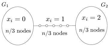
Figure 7: A class of networks and initial conditions for which our algorithm takes $\Theta(n^{2})$ time steps to reach its final state.

References

- [1] D. Angluin, “Local and global properties in networks of processors,” Proceedings of the Twelfth Annual ACM Symposium on the Theory of Computing, 1980.
- [2] J. Aspnes, E. Ruppert, “An introduction to population protocols,” Bulletin of the European Association for Theoretical Computer Science, 93:98-117, 2007.
- [3] T.C. Aysal, M. Coates, M. Rabbat, “Distributed average consensus using probabilistic quantization,” 14th IEEE/SP Workshop on Statistical Signal Processing, 2007.
- [4] Y. Afek,Y. Matias, “Elections in anonymous networks,” Information and Computation, 113(2):113-330, 1994.
- [5] O. Ayaso, D. Shah, M. Dahleh, “Counting bits for distributed function computation,” Proceedings of the IEEE International Symposium on Information Theory, 2008.
- [6] H. Attiya, M. Snir, M.K. Warmuth, “Computing on an anonymous ring,” Journal of the ACM, 35(4):845-875, 1988.
- [7] F. Bénézit, P. Thiran, M. Vetterli, “Interval consensus: from quantized gossip to voting,” Proceedings of ICASSP 08.
- [8] D. Bertsekas, J.N. Tsitsiklis, Parallel and Distributed Computation: Numerical Methods, Prentice-Hall, 1989.
- [9] F. Bullo, J. Cortés, S. Martí nez, Distributed Control of Robotic Networks, Princeton University Press, 2009
- [10] R. Carli, F. Bullo, “Quantized coordination algorithms for rendezvous and deployment,” SIAM Journal on Control and Optimization, 48(3):1251-1274, 2009.
- [11] I. Cidon, Y. Shavitt, “Message terminating algorithms for anonymous rings of unknown size,” Information Processing Letters, 54(2):111–119, April 1995
- [12] M. Draief, M. Vojnovic, “Convergence speed of binary interval consensus,” Proceedings of Infocom 2010.
- [13] P. Frasca, R. Carli, F. Fagnani, S. Zampieri, “Average consensus on networks with quantized communication,” International Journal of Robust and Nonlinear Control, 19(6):1787-1816, 2009.
- [14] F. Fich, E. Ruppert, “Hundreds of impossibility results for distributed computing,” Distributed Computing, 16:121-163, 2003.
- [15] A. Giridhar, P.R. Kumar, “Computing and communicating functions over sensor networks,” IEEE Journal on on Selected Areas in Communications, 23(4):755-764, 2005.
- [16] P. Gacs, G.L. Kurdyumov, L.A. Levin, “One-dimensional uniform arrays that wash out finite islands,” Problemy Peredachi Informatsii, 1978.
- [17] A.G. Greenberg, P. Flajolet, R. Lander, “Estimating the multiplicity of conflicts to speed their resolution in multiple access channels,” Journal of the ACM, 34(2):289-325, 1987.
- [18] Y. Hassin, D. Peleg, “Distributed probabilistic polling and applications to proportionate agreement,” Information and Computation, 171(2):248-268, 2001.
- [19] A. Jadbabaie, J. Lin, A.S. Morse, “Coordination of groups of mobile autonomous agents using nearest neighbor rules,” IEEE Transactions on Automatic Control, 48(6):988-1001, 2003.
- [20] A. Kashyap, T. Basar, R. Srikant, “Quantized consensus,” Automatica, 43(7):1192-1203, 2007.
- [21] E. Kranakis, D. Krizanc, J. van den Berg, “Computing boolean functions on anonymous networks,” Proceedings of the 17th International Colloquium on Automata, Languages and Programming, Warwick University, England, July, 1990.
- [22] N. Khude, A. Kumar, A. Karnik, “Time and energy complexity of distributed computation in wireless sensor networks,” Proceedings of INFOCOM, 2005.
- [23] N. Katenka, E. Levina, G. Michailidis, “Local vote decision fusion for target detection in wireless sensor networks,” IEEE Transactions on Signal Processing, 56(1):329-338, 2008.
- [24] S. Kar, J.M Moura, “Distributed average consensus in sensor networks with quantized inter-sensor communication,” IEEE International Conference on Acoustics, Speech and Signal Processing, 2008.
- [25] N. Lynch, Distributed Algorithms, Morgan-Kauffman, 1996.
- [26] M. Land, R.K. Belew, “No perfect two-state cellular automaton for density classification exists,” Physical Review Letters, 74(25):5148-5150, Jun 1995.
- [27] Y. Lei, R. Srikant, G.E. Dullerud, “Distributed symmetric function computation in noisy wireless sensor networks,” IEEE Transactions on Information Theory, 53(12):4826-4833, 2007.
- [28] L. Liss, Y. Birk, R. Wolff, A. Schuster, “A local algorithm for ad hoc majority voting via charge fusion,” Proceedings of DISC’04, Amsterdam, the Netherlands, October, 2004.
- [29] S. Martinez, F. Bullo, J. Cortes, E. Frazzoli, “On synchronous robotic networks - Part I: models, tasks, complexity,” IEEE Transactions on Robotics and Automation, 52(12): 2199-2213, 2007.
- [30] S. Mukherjee, H. Kargupta, “Distributed probabilistic inferencing in sensor networks using variational approximation,” Journal of Parallel and Distributed Computing, 68(1):78-92, 2008.
- [31] S. Moran, M.K. Warmuth, “Gap theorems for distributed computation,” SIAM Journal of Computing 22(2):379-394, 1993.
- [32] A. Nedic, A. Olshevsky, A. Ozdaglar, J.N. Tsitsiklis, “On distributed averaging algorithms and quantization effects,” IEEE Transactions on Automatic Control, 54(11):2506-2517, 2009
- [33] D. Peleg, “Local majorities, coalitions and monopolies in graphs: a review,” Theoretical Computer Science, 282(2):231-237, 2002.
- [34] E. Perron, D. Vasuvedan, M. Vojnovic, “Using three states for binary consensus on complete graphs,” preprint, 2008.
- [35] L. Xiao, S. Boyd, “Fast linear iterations for distributed averaging,” Systems and Control Letters, 53:65-78, 2004.
- [36] M. Yamashita, T. Kameda, “Computing on an anonymous network,” IEEE transactions on parallel and distributed systems, 7(1):69-89, 1996.
- [37] M. Zhu, S. Martinez, “On the convergence time of asynchronous distributed quantized averaging algorithms,” preprint, 2008.