A multiscale approach to environment and its influence on the colour distribution of galaxies

Abstract

We present a multiscale approach to measurements of galaxy density, applied to a volume-limited sample constructed from the Sloan Digital Sky Survey Data Release 5 (SDSS DR5). We populate a rich parameter space by obtaining independent measurements of density on different scales for each galaxy. This parameterization purely relies on observations and avoids the implicit assumptions involved, e.g., in the construction of group catalogues. As the first application of this method, we study how the bimodality in galaxy colour distribution (specifically $u-r$) depends on multiscale density. The $u-r$ galaxy colour distribution is described as the sum of two gaussians (a red and a blue one) with five parameters: the fraction of red galaxies ($\rm\,f_{red}$) and the position and width of the red and blue peaks ($\rm\,\mu_{red}$, $\rm\,\mu_{blue}$, $\rm\,\sigma_{red}$ and $\rm\,\sigma_{blue}$). Galaxies mostly react to their smallest scale ($<0.5\rm\,Mpc$) environments: in denser environments red galaxies are more common (larger $\rm\,f_{red}$), redder (larger $\rm\,\mu_{red}$) and with a narrower distribution (smaller $\rm\,\sigma_{red}$), while blue galaxies are redder (larger $\rm\,\mu_{blue}$) but with a broader distribution (larger $\rm\,\sigma_{blue}$). There are residual correlations of $\rm\,f_{red}$ and $\rm\,\mu_{blue}$ with $0.5-1\rm\,Mpc$ scale density, which imply that total or partial truncation of star formation can relate to a galaxy’s environment on these scales. Beyond $1\rm\,Mpc$ ($0.5\rm\,Mpc$ for $\rm\,\mu_{red}$) there are no positive correlations with density. However $\rm\,f_{red}$ anti-correlates with density on $>2\rm\,Mpc$ scales at fixed density on smaller scales, and $\rm\,\mu_{red}$ anti-correlates with density on $>1\rm\,Mpc$ scales. We examine these trends qualitatively in the context of the halo model, utilizing the properties of haloes within which the galaxies are embedded, derived by Yang et al. (2007) and applied to a group catalogue. This yields an excellent description of the trends with multiscale density, including the anti-correlations on large scales, which map the region of accretion onto massive haloes. Thus we conclude that galaxies become red only once they have been accreted onto haloes of a certain mass. The mean colour of red galaxies $\rm\,\mu_{red}$ depends positively only on $<0.5\rm\,Mpc$ scale density, which can most easily be explained if correlations of $\rm\,\mu_{red}$ with environment are driven by metallicity via the enrichment history of a galaxy within its subhalo, during its epoch of star formation.

1 Introduction

1.1 Motivation

The evolution of galaxies is heavily intertwined with the growth of the dark matter dominated structure in which they live, as baryons react to their local gravitational potential. It is therefore one of the most challenging goals of observational astronomy to explain the continuously evolving galaxy population in the context of a hierarchical universe. Most fundamentally perhaps, galaxies exhibit a distinct bimodality of properties which correlates strongly with the properties of the embedding potential. This is true whether the potential is measured on galaxy scales via properties such as luminosity, stellar or dynamical mass, or on larger scales via measurement of the galaxies’ local environment. In particular, galaxies living in deeper potential wells are more likely to have formed stars at earlier times, both in terms of the average stellar age (e.g. Thomas et al., 2005; Smith et al., 2006) and the last episode of star formation (and thus a lower fraction are continuing to form stars, e.g. Lewis et al., 2002; Baldry et al., 2004; Balogh et al., 2004a, b; Kauffmann et al., 2004). Such galaxies are apparently unable to restart star formation, since they have no stable access to a suitable reservoir of gas which can cool to form a star-forming disk (e.g. Gallagher et al., 1975; Caon et al., 2000). Simultaneously the morphology of these galaxies must evolve from the typical rotation-dominated spiral or irregular morphologies of star-forming galaxies to form a pressure dominated elliptical, or a bulge plus smooth disk lenticular (e.g. Dressler, 1980; Dressler et al., 1997; Wilman et al., 2009). The precise nature of these transformations remains controversial, despite evidence from simulations and observations for various mechanisms which can explain some or all of these observations. Galaxy mergers are especially attractive in the context of a hierarchical Universe, and can explain both morphological changes and the rapid exhaustion of cold gas, although additional physics may be required to keep a galaxy from reforming a gas disk (e.g. Springel et al., 2005; Hopkins et al., 2009; Johansson et al., 2009). Stripping or evaporation of cold and/or hot gas associated to an infalling galaxy will take place within a dense hot intra-cluster medium (e.g. Gunn & Gott, 1972; Chung et al., 2009; Larson et al., 1980), although it is unclear whether these processes can be important within lower density environments (Kawata & Mulchaey, 2008; McCarthy et al., 2008; Jeltema et al., 2008). Tidal interactions between galaxies can drive gravitational instabilities within galaxies, with gas loss or triggering of star formation as likely consequences. Numerous fast interactions (harrassment) can also drive morphological evolution (e.g. Moore et al., 1999).

To statistically describe the evolutionary path of galaxies, it is necessary not only to take a firm grasp of the relevant physical processes but also to place robust observational constraints on precisely how the galaxy population reacts to its environment. It has been customary in this field to use neighbouring galaxies as test particles in order to ‘measure’ the local environment of each galaxy. One computes a ‘local density’ by simply counting neighbours within some fixed radius and velocity range or, almost equivalently, by computing the distance to the N^th nearest neighbour, where N is typically chosen to be 5 or 10 (Dressler (1980); Balogh et al. (2004a), see Cooper et al. (2005); Kovac et al. (2009) for a discussion of these and more complex methods). As with so many traditional measures, this measurement is fairly arbitrary in nature , and it is not easy to see precisely how it relates to the underlying density field of galaxies and dark matter.

The two point correlation function or power spectrum of galaxies on the other hand, measure the excess probability over random of finding two galaxies with a given separation. The comparison of galaxy subsets selected by e.g. colour, provides a measure of the relative bias of these galaxy types as a function of the scale of pair separation, diagnosing the scale at which one class dominates relative to another. (e.g. Norberg et al., 2001; Budavári et al., 2003; Zehavi et al., 2005). Marked correlation functions weight the galaxies in each pair by a given property, normalizing by the unweighted correlation function (e.g. Skibba et al., 2006). This examines how galaxies with large or small values of the chosen property are clustered. The bias or marked correlation as a function of scale are intimitely related to the details of how galaxy properties depend on their environments.

These statistics simply provide the mean behaviour of galaxies by tracing their overdensity on different scales which, however, are themselves closely correlated with one another. A better approach would be to examine how galaxy properties correlate with overdensity on one scale for a fixed overdensity on another, independently computed scale. Now that such a large, homogeneous sample of galaxies is available with the Sloan Digital Sky Survey (SDSS), there have been a few attempts at isolating such behaviour on different scales. Kauffmann et al. (2004), Blanton et al. (2006) and Blanton & Berlind (2007) conclude that galaxies only react to their environments on $<1\rm\,Mpc$ scales, with no significant residual dependence on larger scale overdensity. This contradicts the apparent dependence on large scales found by Balogh et al. (2004a), which may have resulted from low signal to noise measurement of density on small scales (Blanton et al., 2006). These works, however, contained correlated measurements of density on both scales.

1.2 A New Method

In this paper we approach this problem in a different way. Firstly, we parameterize the environment using annular, non-overlapping measurements of density on different scales to ensure that they are (formally) independent. Secondly, we consider the $u-r$ colour of galaxies and utilize the remarkable fact that its distribution is bimodal and can be modelled as the sum of two gaussians. This relates to the bimodality of galaxy properties, since galaxies dominated by old stellar populations have red $u-r$ colours and actively star-forming galaxies are blue. Baldry et al. (2004) initially demonstrated the power of this technique, illustrating the low chi-squared values produced with such a fit to $u-r$ SDSS colours, and demonstrating that the luminosity dependence of galaxy colours was strong and easily parameterized using this model. Balogh et al. (2004b) and Baldry et al. (2006) have since extended this method, with a powerful demonstration of the strong and fundamental dependence of the fraction of red galaxies on environment (measured using the distance to the $4^{th}$ and $5^{th}$ nearest neighbours) and stellar mass. The parameterization of the double gaussian fit (the fraction of red galaxies $\rm\,f_{red}$, and the position and width of each peak) provides five quantities which can be interpreted in terms of changes in the spectral energy distribution and the potential physical trigger, and which can be correlated with environment measured on different scales.

1.3 Expectations from the Halo Model

Finally, to ease the physical interpretation of our results, we would like to know how measurements of density map onto the dark matter dominated ‘cosmic web’. To this goal we rely on the models that describe the clumpy distribution of dark matter in the Universe in terms of haloes, i.e. the potential wells in which galaxies form, infall, virialize and interact with one another and with the intra-cluster/group medium (ICM/IGM) (e.g. White & Rees, 1978; Cooray & Sheth, 2002; Diaferio et al., 2001). The halo model (which applies on both galaxy and group/cluster scales) is a simplification of reality, but has been hugely successful in describing the dynamics and large scale structure statistics of galaxies (e.g. Rubin, 1983; Berlind et al., 2003). In particular, the two point correlation function appears to demonstrate an inflection at $\sim 2\rm\,Mpc$ which is attributed to the switch from sub-halo scales (the one halo term) to halo-halo scales (the two halo term) (e.g. Zehavi et al., 2004, 2005; Cooray, 2006). Models of galaxy formation and evolution pay homage to the halo model by assuming galaxies to care about their environment only in terms of their embedding dark matter halo (e.g. Kauffmann et al., 1993; Cole et al., 2000). This puts a natural scale on the expected dependence of galaxy properties on their environments: they should not care about scales beyond their halo. However simulations also show that the formation (collapse) time of a halo depends upon the overdensity on larger scales (e.g. Sheth & Tormen, 2004; Gao et al., 2005). In this case, one might expect galaxies to have evolved further in a region of the Universe which is more overdense on large scales.

1.4 Structure of the paper

Section 2 introduces the sample used in this paper, selected from the SDSS Data release 5 (DR5). In Section 3 we describe in detail the method used to compute the density of galaxies on different scales, paying close attention to the completeness corrections required to ensure a robust measurement in the presence of incompleteness in SDSS DR5.

Multiscale density information for the 73662 galaxies of our photometrically complete sample are available for public use on request to the authors.

The method of fitting a double gaussian model is described in Section 4. Our results are presented in Section 5. Firstly we examine the simple dependence of the galaxy colour distribution on luminosity and density on a single scale in Section 5.1. Then, in Section 5.2, we present our main results in which the importance of different scales are tested independently. This forms the purely observational part of the paper.

In Section 6 we utilize a catalogue of embedding haloes (groups) which has been assigned to SDSS galaxies within the context of a halo model and with a few implicit assumptions (Yang et al., 2007). We examine the dependence of halo-based properties such as mass and halo-centric radius on the density computed on different scales and compare this to the way in which the galaxy colour distribution depends upon the same measurements of density. What emerges is a remarkably consistent picture, in which the halo model is extremely successful at explaining the colours of galaxies: smaller scale density can drive some aspects of colour evolution, but star forming galaxies do not seem to feel the halo environment prior to infall. This exercise should provide the first, qualitative step towards a fully quantative, model-independent description of the way in which galaxies trace their environment. Models can then be constrained independently of the assumptions that are required in the construction of group catalogues or modeling of the correlation function. The rich parameter space of multiscale densities will help overcoming degeneracies and difficulties in interpreting single aperture measurements of local density.

In this paper we assume the cosmological parameters: $(\Omega_{M},\Lambda,h)=(0.3,0.7,0.75)$.

2 Sample

We base our analysis on the Fifth Data Release (Adelman-McCarthy et al., 2007, DR5) of the Sloan Digital Sky Survey (York et al., 2000, SDSS). We define an initial sample of galaxies with a valid spectroscopic redshift determination, which are part of the so-called ‘main galaxy sample’ (i.e. all extended sources with petrosian dereddened magnitude brighter than 17.77 in $r$-band and mean surface brightness within half-light radius $\mu_{r}\leq 23.0$ mag arcsec^-2, see Strauss & et al. 2002). This sample covers 5713 square degrees. We further restrict the selection to the redshift range $0.015\leq z$: the lower limit is chosen such that local deviations from the Hubble flow negligibly affect distance estimates.

For this sample we compute the two photometric quantities relevant to the present work, namely the rest-frame de-reddened Petrosian $r$-band (absolute) magnitude and the rest-frame model colour $u-r$. De-reddening is based on the estimate of foreground Galactic extinction derived by Schlegel et al. (1998), while the transformation to rest-frame quantities is performed using the software k-correct (v4.1.3 Blanton & Roweis, 2007), based on the five-band $u,g,r,i,z$ spectral energy distribution (see Fukugita et al., 1996, for details on the SDSS photometric system). By choosing the petrosian magnitude as a base and proxy for the total galaxy luminosity we provide that the SDSS selection criteria simply propagate in our sample selection and binning, and at the same time we avoid redshift dependent biases in the estimate of the total luminosity (this derives from the definition of petrosian magnitude, Petrosian 1976). On the other hand, as noted in Stoughton & et al. (2002), the so-called SDSS model magnitudes are best suited to derive colours, as they are computed with a weighted aperture photometry scheme common to all five bands, which ensures results that are independent on the wildly different signal-to-noise ratio in each band. The choice of the $u-r$ colour among all possible combinations of the five SDSS pass-bands appears optimal to study galaxy bimodality (as shown, e.g., in Baldry et al., 2004): the physical reason is that $u-r$ provides a long wavelength leverage (therefore it is very sensitive to the shape of the optical SED, depending on star formation history, metallicity and dust extinction) across the 4000Å-break (which is the strongest spectral feature at optical wavelengths and responds mainly to changes in stellar population age).

The upper panel of Figure 1 illustrates the Petrosian r-band luminosity $M_{r}$ as a function of redshift $z$ for a random subsample of our galaxies. The spectroscopic selection threshold at a luminosity corresponding to apparent magnitude $m_{r}=17.77$ is a strong function of redshift, and a weak function of SED type at given redshift (k-correction). This is better illustrated in the lower panel where we show the k-corrected magnitude not corrected for the distance modulus, as a function of redshift. To assess the effect of the k-correction on the luminosity limit, the percentiles of the k-correction distribution are computed as a function of redshift, and are applied at the magnitude limit. The solid blue and dashed green lines show the 95^th and 50^th percentiles respectively, which clearly become larger with redshift as the k-corrected magnitude limit diverges from the non-corrected limit of $m_{r}=17.77$ (magenta dashed line).

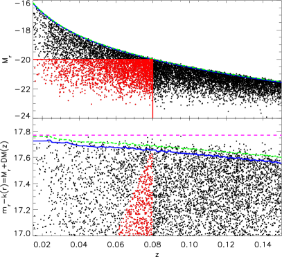
Figure 1: Sample selection in top: dereddened Petrosian luminosity $M_{r}$ vs redshift and bottom: k-corrected dereddened Petrosian magnitude $m_{r}$ vs redshift for a random selection of galaxies in the sample. Galaxies in the volume-limited sample ($z\leq 0.08$ and $M_{r}\leq-20.0$) are highlighted in red. The blue solid line corresponds to the 95${}^{th}\%$ile of the k-correction distribution at the magnitude limit of $m_{r}=17.77$. The dashed green line is equivalent, only for the 50${}^{th}\%$ile of the k-correction distribution, whilst the dashed magenta line illustrates the magnitude limit (no k-correction).

To study environment, it is important that the luminosity limit for each galaxy and its neighbours (which will be used to estimate the local environmental density) is the same, regardless of distance. Therefore, a volume-limited sample with a constant luminosity limit as a function of redshift is required. Similar to Balogh et al. (2004b), we find that a suitable compromise between volume and depth can be achieved by limiting to $z\leq 0.08$ and $M_{r}\leq-20.0$. Galaxies meeting these criteria are plotted red in Figure 1, and within the region delineated by the solid red lines in the luminosity-redshift plane (upper panel). All galaxies with k-corrections less than the 95^th percentile of the distribution, and Petrosian r-band luminosities $M_{r}\leq-20.0$ will be potential spectroscopic targets out to $z=0.08$, providing a measure of environment. The most extreme galaxies with the upper 5% of k-corrections may still be missed at redshifts very close to $z=0.08$. However these will by definition be extremely few and with perhaps the least reliable k-corrections.

The volume-limited sample contains 92082 galaxies, with a median redshift of 0.066.

3 Measurement of density on different scales

The goal of this paper is to test the correlation between the galaxy colour bimodality and the environmental density on different scales, which we measure as follows. A cylindrical annulus, centred on each galaxy in the volume-limited sample, is used to measure the local projected density of neighbouring galaxies above the limiting luminosity between an inner and outer radius and within a fixed rest-frame velocity range. By selecting non-overlapping annuli we can extract complimentary information about the overdensity of galaxies on different scales, which will only correlate with each other because the underlying density field correlates on different scales, coupled with the effects of projection and redshift distortions. For an annulus with inner radius $r_{i}$ and outer radius $r_{o}$, the surface density $\rm\,\Sigma_{r_{i},r_{o}}$ is given by:

$$\rm\,\Sigma_{r_{i},r_{o}}=\frac{\rm\,N^{n}_{r_{i},r_{o}}}{\pi(r_{o}^{2}-r_{i}^{2})}$$ (1)

where $\rm\,N^{n}_{r_{i},r_{o}}$ is the completeness-corrected number of neighbours brighter than our limit, within the rest-frame velocity range $\pm dv$, and with a projected distance from the primary galaxy $r$ where $r_{i}\leq r\leq r_{o}$. For the purposes of this paper we choose neighbours brighter than the volume-limited sample depth of $M_{r}=-20.0$ and within $dv=1000kms^{-1}$ of the primary galaxy. This is equivalent to that used by Balogh et al. (2004b), sampling $\pm\sim 1\sigma$ for massive clusters in velocity space, or a redshift space cylinder of length $\pm\sim 14\rm\,Mpc$. On large scales this traces the non-linear regime for high densities, whilst voids remain underdense ($\sim 1\%$ of galaxies have zero neighbours within $r_{o}=3\rm\,Mpc$).

3.1 Selection and Correction for Completeness

In order to estimate local galaxy densities properly, selection effects must be taken into account and completeness corrections applied. In the first place, we request the photometric coverage of the region used to compute local density to be highly complete. We compute the photometric completeness within a $3\rm\,Mpc$ circle centred on each galaxy in the volume-limited sample, at the redshift of the galaxy. Using the same tools that also power the spatial computations within the National Virtual Observatory’s Footprint Service (Budavári et al., 2007), we perform the formal algebra of the relevant spherical shapes on the sky. The 3Mpc circle is first intersected with the sky coverage of the DR5 survey that yields the observed area. Furthermore we have to censor problematic regions due to nearby bright stars, bleeding, satellite trails and missing fields. The Sloan collaboration provides spherical polygons of these masks that one has to exclude by subtracting their shapes from the observed area. In addition, we also censor out bad seeing patches that are worse than 1.7$\arcsec$ in the r band. Using the Spherical Library (Budavári, 2009), we compute the exact shape of every cell, and analitically calculate its area. The completeness is then just the ratio of this area to the full circle.

The resultant cumulative distribution of photometric completeness shows two regimes with 80% of the galaxies having completeness above 98.645%. This is an acceptable loss of area which will only have minimal effects on our density estimates. The remaining 20% of galaxies have much less complete photometry within 3$\rm\,Mpc$. This is where the edge effects of the SDSS coverage become important. We keep the 80% of galaxies with better than 98.645% photometric completeness, for which the residual incompleteness can be attributed to regions removed due to bright stars, satellite / asteroid trails and imaging defects. This leaves us with a sample of 73662 galaxies.

Local density estimates are obviously affected by the spectroscopic incompleteness of the survey, which is likely to depend upon environment. In fact, due to fiber collision effects (i.e. fibers could not be assigned to targets within 55″ of each other) spectroscopic observations are biased against galaxies in denser regions of the sky. For example, $\sim 10\%$ of galaxies with $\rm\,\Sigma_{0,0.5}\geq 23\rm\,Mpc^{-2}$ are missing spectra for half their potential neighbours. It is possible to correct statistically for the spectroscopic incompleteness effects by computing a correction factor for the number of neighbours, based upon the fraction of targets with a valid redshift measurement.

The spectroscopic completeness correction factor is computed on a range of different scales:

$$\rm\,C^{s}_{r_{i},r_{o}}=\frac{\rm\,N^{p}_{r_{i},r_{o}}}{\rm\,N^{s}_{r_{i},r_{o}}}$$ (2)

where $\rm\,N^{p}_{r_{i},r_{o}}$ is the total number of photometrically identified spectroscopic targets within the annulus and $\rm\,N^{s}_{r_{i},r_{o}}$ is the number with redshift. This factor corrects for the incomplete sampling of galaxies within dense regions, up-weighting the number of neighbours in equation 1 such that:

$$\rm\,N^{n}_{r_{i},r_{o}}=\rm\,C^{s}_{r_{i},r_{o}}\times\rm\,N^{un}_{r_{i},r_{o}}$$ (3)

where $\rm\,N^{un}_{r_{i},r_{o}}$ is the uncorrected number of redshift space neighbours within our radial, velocity and luminosity constraints.

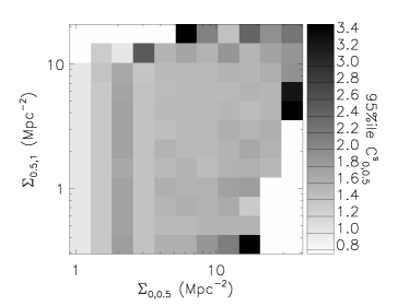
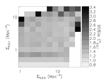
Figure 2: 95%ile of the completeness corrections $\rm\,C^{s}_{0,0.5}$ and $\rm\,C^{s}_{0,1}$ as a function of $\rm\,\Sigma_{0,0.5}$ and $\rm\,\Sigma_{0.5,1}$. Larger completeness corrections are required at high density, where fiber allocation is difficult. Quantized neighbours lead to “stripes” of high $C^{s}$ in particular lower density bins.

Figure 2 illustrates how $\rm\,C^{s}_{0,0.5}$ and $\rm\,C^{s}_{0,1}$ depend upon $\rm\,\Sigma_{0,0.5}$ and $\rm\,\Sigma_{0,1}$. We take the 95%ile of the distribution to examine the largest corrections in each bin of density. As expected, the largest corrections exist at high density due to fiber collision effects, although at low densities the quantized number of neighbours combined with finite binning leads to artificial selection of high completeness galaxies in particular bins (striping).

Galaxies with no known neighbours ($\rm\,N^{un}_{r_{i},r_{o}}=0$) will automatically also have no neighbours in the completeness-corrected density ($\rm\,\Sigma_{r_{i},r_{o}}=0$), regardless of the completeness correction ($\rm\,C^{s}_{r_{i},r_{o}}$). In theory this means a galaxy with many neighbours can still have $\rm\,\Sigma_{r_{i},r_{o}}=0$ if all true neighbours have no redshift information. However, only $\sim 4\%$ of galaxies with one known neighbour within $3\rm\,Mpc$ ($\rm\,N^{un}_{0,3}=1$) have completeness correction larger than 50% ($\rm\,C^{s}_{0,3}>1.5$). Therefore completeness corrections are typically not large for galaxies in low density regions, and it is unlikely that the signal from galaxies with $\rm\,\Sigma_{r_{i},r_{o}}=0$ is dominated by galaxies which truly have significantly larger densities.

4 Fitting Method

We parameterize the galaxy colour distribution as a double gaussian, as illustrated by Baldry et al. (2004), Balogh et al. (2004b) and Baldry et al. (2006), to examine the dependence of the galaxy colour distribution on galaxy luminosity and environment on different scales. The colour distribution $\Phi(C)$ for a given sample of $N_{T}$ galaxies is thus fit by the following function:

$$\Phi(C)=\frac{\rm\,f_{red}N_{T}}{\sqrt{2\pi}\rm\,\sigma_{red}}e^{\frac{-(C-\rm\,\mu_{red})^{2}}{2\rm\,\sigma_{red}^{2}}}+\frac{(1-\rm\,f_{red})N_{T}}{\sqrt{2\pi}\rm\,\sigma_{blue}}e^{\frac{-(C-\rm\,\mu_{blue})^{2}}{2\rm\,\sigma_{blue}^{2}}}$$ (4)

where the five relevant parameters are: the fraction of red galaxies $\rm\,f_{red}$ and the mean colours and widths of the red and blue peaks $\rm\,\mu_{red}$, $\rm\,\mu_{blue}$, $\rm\,\sigma_{red}$ and $\rm\,\sigma_{blue}$.

Our fitting procedure for any given sample is based upon the one outlined in Section 4 of Baldry et al. (2004). Here we summarize it and describe the details specific to our analysis.

The galaxies are binned in colour, with a bin width of 0.1 magnitudes. The fit is limited to the range $0.75\leq u-r\leq 3.0$.

The double gaussian model is then fit to the binned colour distribution using a Levenberg-Marquardt least-squares fit. In doing this, each colour bin is weighted by the inverse variance, computed as the square of the Poisson error plus a softening factor of two ($W=\frac{1}{N+2}$). Bins containing no galaxies are weighted equivalently to bins with one galaxy ($W=\frac{1}{3}$).

Low number statistics can produce noisy colour distributions, and so additional constraints need to be placed upon the fits, and initial estimates of the parameters given, in order to prevent the fitting algorithm from converging to false minima. Most importantly, we only fit samples of at least 25 galaxies, which extensive testing shows recovers sensible results. Initial estimates of $\mu$ and $\sigma$ are taken from the fit parameterized in Table 1 of Baldry et al. (2004). An estimate of $\rm\,f_{red}=0.5$ is applied to the brightest bin with estimates for each successive bin of luminosity taking the value computed for the previous bin. Once each luminosity bin is split into bins of density, the initial parameter estimates are set to the values computed for the full bin. The results are insensitive to the precise values selected. The blue peak is constrained such that $\rm\,\mu_{blue}$ cannot be less than 0.2$mag$ bluer than the initial estimate of $\rm\,\mu_{red}$. This ensures that the two peaks remain separate entities, and do not switch places. Finally, we also constrain the widths ($\rm\,\sigma_{red}$, $\rm\,\sigma_{blue}$) to be within the range $0.05\leq\sigma\leq 0.8$. This avoids pathological solutions in cases where the colour distribution exhibits large noise spikes or unusually large number of galaxies in the tails of the distribution.

In all cases good fits are achieved, yielding reduced chi-squared values near or below unity. As discussed by Baldry et al. (2004), the softening factor of two privides an approximation to the uncertainties involved for low number counts with a Poisson distribution. Inevitably this approximation, combined with the finite weighting of bins containing no counts, leads to frequent cases of reduced chi-squared significantly less than one. In the following analysis errors on the $\rm\,f_{red}$ are computed purely statistically, and are insensitive to (but consistent with) the fitting errors. Errors on the other parameters are estimated from fitting. In these cases it was necessary to multiply the error on each parameter by $\sqrt{(}\chi_{red}^{2})$ since the errors on these parameters are overestimated for $\chi_{red}^{2}<1$ (propogated from overestimated errors on the datapoints). Whilst this is clearly an approximate correction, we note that the fit errors on these parameters are only applied in Figures 4 and 5, and that our main conclusions are based instead on the correlation with density of properties computed in independent bins.

5 Results

5.1 Dependence on Luminosity and Density

A large number of galaxies per luminosity bin are required to examine the multiscale density dependence of galaxy properties within that bin. Therefore we limit our analysis to the luminosity range $-21.5\leq\rm\,M_{r}\leq-20.0$.

The top panels in Figures 3, 4 and 5 illustrate the dependence of the five parameter family ($\rm\,f_{red}$, $\rm\,\mu_{red}$, $\rm\,\mu_{blue}$, $\rm\,\sigma_{red}$, $\rm\,\sigma_{blue}$) on luminosity, $\rm\,M_{r}$, as resulting from the fitting procedure applied to the volume-limited sample within this luminosity range. We confirm the results of Baldry et al. (2004) indicating that all five parameters are strong functions of luminosity: lower luminosity galaxies display a lower fraction of red galaxies, bluer mean colours for both peaks and a broader red peak but narrower blue peak than do more luminous galaxies within the range considered. Small differences from Baldry et al. (2004) result from improved k-corrections (a later version of the k-correct code was used). There is no measurable dependence of colour ($\rm\,\mu_{red}$ or $\rm\,\mu_{blue}$) for constant luminosity galaxies on redshift, indicating that the k-corrections are consistent across our small redshift range. We note that, for the luminosity range sampled by the volume-limited sample, the fraction of red galaxies $\rm\,f_{red}$ is only weakly dependent on luminosity, while both $\mu$ and $\sigma$ show strong variation for both peaks. This luminosity dependence of these properties within the volume-limited sample is consistent with that obtained for a larger sample with variable redshift limit as a function of galaxy luminosity.

Residual quantities ($\rm\,\Delta(f_{red})$, $\rm\,\Delta(\mu_{red})$, $\rm\,\Delta(\mu_{blue})$, $\rm\,\Delta(\sigma_{red})$, $\rm\,\Delta(\sigma_{blue})$) are defined for each subsample (sub) as follows:

$$\rm\,\Delta(f_{red})=\rm\,f_{red}(\rm\,M_{r},sub)-\rm\,f_{red}(\rm\,M_{r})$$ (5)

$$\rm\,\Delta(\mu)=\mu(\rm\,M_{r},sub)-\mu(\rm\,M_{r})$$ (6)

$$\rm\,\Delta(\sigma)=\sigma(\rm\,M_{r},sub)-\sigma(\rm\,M_{r})$$ (7)

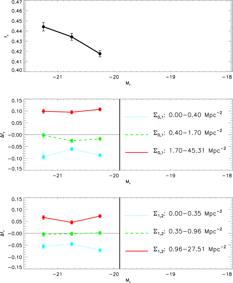
Figure 3: Top: $\rm\,f_{red}$ as a function of luminosity, $\rm\,M_{r}$, for the full volume-limited sample in the luminosity range of interest. Middle: Residuals for different bins of $\rm\,\Sigma_{0,1}$. Bottom: and in different bins of larger scale density, $\rm\,\Sigma_{1,2}$. Errors are computed using the Gehrels (1986) approximation, combining Poissonian and Binomial statistical errors. For double gaussian fits to a large number of galaxies this approximates the fitting error, whilst for smaller numbers the statistical error is larger.

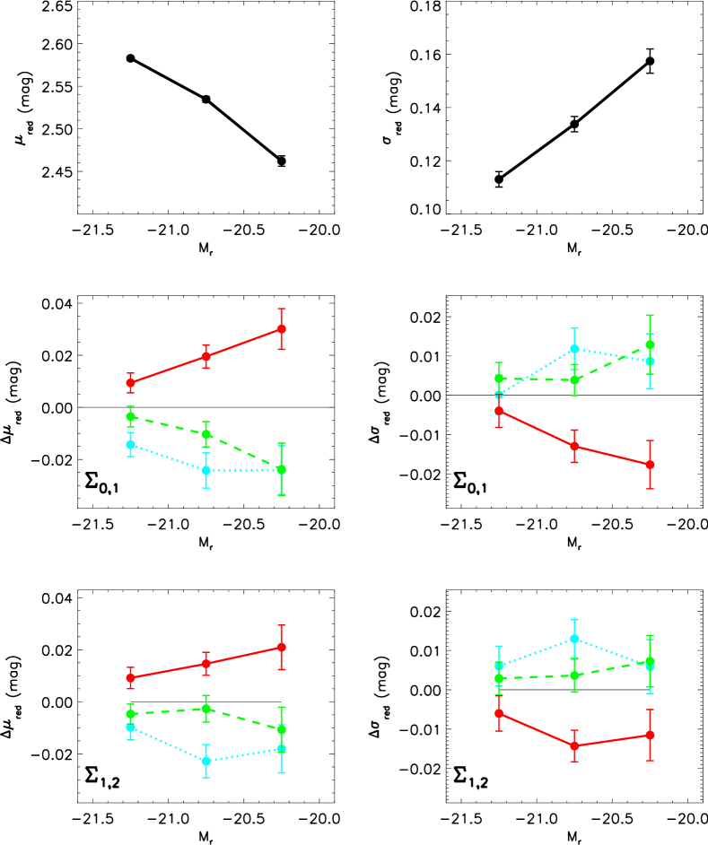
Figure 4: Top: $\rm\,\mu_{red}$ and $\rm\,\sigma_{red}$ as a function of luminosity, $\rm\,M_{r}$, for the full volume-limited sample in the luminosity range of interest. Middle: Residuals for different bins of $\rm\,\Sigma_{0,1}$. Bottom: and in different bins of larger scale density, $\rm\,\Sigma_{1,2}$. Errors are pure fitting errors. Key as in Figure 3.

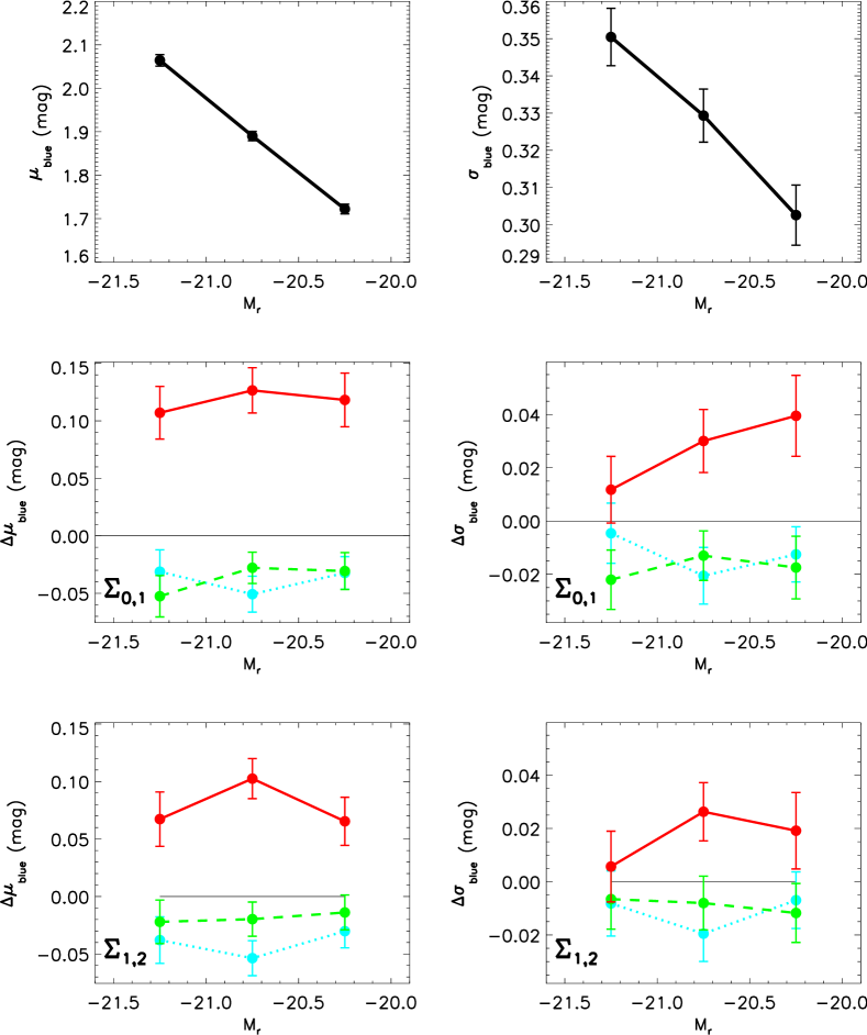
Figure 5: Top: $\rm\,\mu_{blue}$ and $\rm\,\sigma_{blue}$ as a function of luminosity, $\rm\,M_{r}$, for the full volume-limited sample in the luminosity range of interest. Middle: Residuals for different bins of $\rm\,\Sigma_{0,1}$. Bottom: and in different bins of larger scale density, $\rm\,\Sigma_{1,2}$. Errors are pure fitting errors. Key as in Figure 3.

The middle and lower panels of Figures 3, 4 and 5 show how these quantities depend upon luminosity for three bins of density on $<1\rm\,Mpc$ scales ($\rm\,\Sigma_{0,1}$, middle panels) and $1-2\rm\,Mpc$ scales ($\rm\,\Sigma_{1,2}$, lower panels). These density bins contain the upper, middle and lower thirds of the density distribution on these scales, and the whole volume-limited sample is represented in black.

The density dependence of the colour distribution on both small and large scales is extremely clear in these figures:

• The fraction of red galaxies is a strong function of environment, with a difference in $\rm\,f_{red}$ between the most and least dense thirds of the distribution ranging from 0.15 to 0.19 and from 0.09 to 0.15 for densities computed on $<1\rm\,Mpc$ and $1-2\rm\,Mpc$ scales, respectively. This is almost independent of luminosity in the range $-21.5\leq\rm\,M_{r}\leq-20.0$.

• The characteristics of the red peak are also highly significant functions of environment, although the dynamic range is smaller than for the luminosity dependence. The difference in the mean colour $\rm\,\mu_{red}$ for the most and least dense thirds of the distribution on $<1\rm\,Mpc$ scales is in the range 0.02 to 0.06 mag. In the most overdense regions, in going to fainter luminosity $\rm\,\Delta(\mu_{red})$ increases (becomes redder), whilst the relative width of the peak $\rm\,\Delta(\sigma_{red})$ simultaneously decreases. A similar range but with less obvious luminosity dependence is observed using densities on $1-2\rm\,Mpc$ scales.

• The blue peak properties $\rm\,\mu_{blue}$ and $\rm\,\sigma_{blue}$ are more strongly correlated with environment than the equivalent red peak properties. A difference in $\rm\,\mu_{blue}$ of 0.15 to 0.18 mag between the most and least dense bins on $<1\rm\,Mpc$ scales is present at all luminosities. The difference is still significant but slightly smaller using density on $1-2\rm\,Mpc$ scales. $\rm\,\sigma_{blue}$ is also dependent on density in the sense that the blue peak appears broader for galaxies in denser environments, possibly more so at fainter luminosities.

To demonstrate the reality of these trends, we show the actual colour distributions with overplotted fits in Figure 6. The strong luminosity dependence of $\rm\,\mu_{blue}$, $\rm\,\sigma_{blue}$, $\rm\,\mu_{red}$ and $\rm\,\sigma_{red}$ and the density dependence of $\rm\,f_{red}$ are immediately obvious. To better illustrate the differences, the values of $\rm\,\mu_{blue}$ and $\rm\,\mu_{red}$ are marked as dashed vertical lines. Similarly the density dependence of $\rm\,\sigma_{blue}$ and $\rm\,\sigma_{red}$ can be seen by comparing the actual fit with the fit as it would be if $\sigma$ was fixed to the values computed for the lowest density bin (overplotted dotted lines). It is apparent, especially in the faintest, highest density bin (lower right) and for $u-r$ near $\rm\,\mu_{blue}$ and $\rm\,\mu_{red}$ that a broader blue peak and narrower red peak are required. Masjedi et al. (2006) find that very nearby neighbours (within $\sim 20\arcsec$) significantly influence the measured luminosity of galaxies: however model colours are likely to be much more robust. In any case, whilst $\rm\,\sigma_{blue}$ increases at high density, this is unlikely to be related to increased photometric errors: $\rm\,\sigma_{red}$ should be as influenced but decreases, whilst the $\sim 20\%$ drop in the amplitude of the blue distribution (bottom right panel of Figure 6, compare solid and dashed lines) is too strong to be caused by such a rare population of very close neighbours. It must be noted that for such well populated samples there are small but mildly significant deviations from a perfect double gaussian distribution, visible as assymetries in the distribution or an excess of galaxies at intermediate colours. Whilst these deviations are potentially interesting, they are so small that they can and should be ignored in the context of this paper.

       

       

       

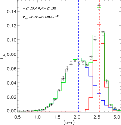
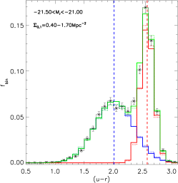
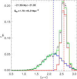
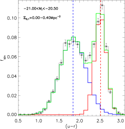
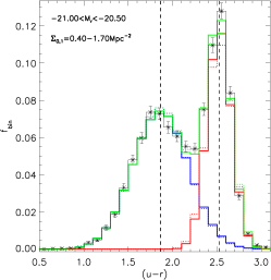
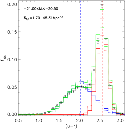
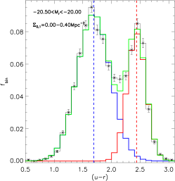
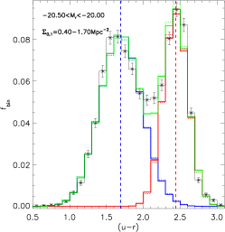
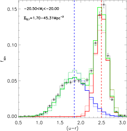
Figure 6: $u-r$ colour distribution of galaxies (points and black solid line) as a function of luminosity and density, with double gaussian fits (red$+$blue peak$=$green line). Top to bottom: Decreasing luminosity $\rm\,M_{r}=-21.5$ to $-20.0$ in bins of $0.5$mag width. Left to right: Underdense to overdense, split evenly into bins by $\rm\,\Sigma_{0,1}$. Overplotted is the mean colour for each peak (vertical lines), indicating that both peaks move redwards going to higher density. Also overplotted (dotted lines) is the sum of two gaussians with equivalent parameters, except the widths ($\rm\,\sigma_{blue}$,$\rm\,\sigma_{red}$) are fixed to the value computed for the lowest density bins (left panels). The deviation in the highest density bins illustrates the dependence of $\sigma$ on density (strongest in the faintest bin, lower right).

The similar dependence of $\rm\,f_{red}$ on density across this luminosity range (i.e., no luminosity dependence for $\rm\,\Delta(f_{red})$) is in qualitative agreement with Balogh et al. (2004b), although they appear to measure a larger dynamic range for $\rm\,f_{red}$ as a function of the surface density within the $5^{th}$ nearest neighbour, $\Sigma_{5}$, at fixed luminosity. Binning more finely in density, we find that the increase in $\rm\,\Delta(f_{red})$ for galaxies in the highest density third is mainly contributed by a small fraction of galaxies ($\sim 15\%$) with $\rm\,\Sigma_{0,1}\gtrsim 4.0\rm\,Mpc^{-2}$. It is also noticeable that the trends of $\rm\,\Delta(\mu_{red})$ and $\rm\,\Delta(\mu_{blue})$ with density are quantitatively comparable to the Balogh et al. (2004b) results, with more extreme values when more extreme (rare) environments are isolated.

A detailed interpretation of our results will be left for Section 6. For now we note that Figure 3 suggests that suppression of star formation leads to the formation of red galaxies preferentially in environments characterized by a high local ($<1\rm\,Mpc$ scale) density. The importance of different scales will be addressed in Section 5.2. The dependence of $\rm\,\mu_{red}$ and $\rm\,\sigma_{red}$ on environment could relate to differences in either/both age or/and metallicity of the stellar population, although intragalactic dust in galactic and group scale haloes can account for part of the effect ($\lesssim 0.01$ mag, Ménard et al., 2009; McGee & Balogh, 2009). A plausible scenario is that less luminous galaxies in dense environments will typically be satellites, which may have experienced early suppression of their star formation. Such galaxies will have an older and purer underlying population than similar galaxies in lower density environments, leading to redder colours and smaller scatter (i.e. smaller $\rm\,\sigma_{red}$). Meanwhile the redder, broader blue peak in dense environments suggests a more disturbed and (on average) less active recent star formation history compared to those in less dense environments, although internal dust extinction may also play a role.

5.2 Scale Dependence

Figures 3, 4 and 5 illustrate that whilst the colour distribution of galaxies depends upon density on $<1\rm\,Mpc$ scales, $\rm\,\Sigma_{0,1}$, it also depends (to a smaller extent) on a totally independent measurement of density on larger scales, $\rm\,\Sigma_{1,2}$. However, although $\rm\,\Sigma_{1,2}$ is measured independently of $\rm\,\Sigma_{0,1}$, the two quantities are nonetheless strongly correlated. This is illustrated in Figure 7, in which we show the distribution of $-21.5<\rm\,M_{r}<-20.0$ galaxies on density computed on the different scales that we will consider in our analysis. Binning is logarithmic in density, with less than 50% density increase within each bin on either scale except the highest and lowest density bins, which have infinity and 0 as upper and lower boundaries, respectively. The left panel examines the distribution in the $\rm\,\Sigma_{0,0.5}$ versus $\rm\,\Sigma_{0.5,1}$ plane, whilst successively larger scales are examined in the $\rm\,\Sigma_{0,1}$ versus $\rm\,\Sigma_{1,2}$ and $\rm\,\Sigma_{0,2}$ versus $\rm\,\Sigma_{2,3}$ planes in the central and right panels respectively.

       

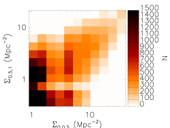
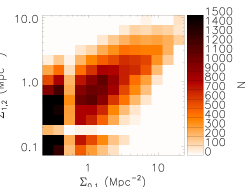
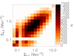
Figure 7: Number of $\-21.5<\rm\,M_{r}<-20.0$ galaxies binned in two independently measured scales of density. Left: on scales $\rm\,\Sigma_{0,0.5}$ and $\rm\,\Sigma_{0.5,1}$; Centre: on scales $\rm\,\Sigma_{0,1}$ and $\rm\,\Sigma_{1,2}$; Right: on scales $\rm\,\Sigma_{0,2}$ and $\rm\,\Sigma_{2,3}$. Small and large scale densities are strongly correlated with each other.

The strong correlation between small and large scale densities at $<3\rm\,Mpc$ probes the non-linear regime of collapse which amplifies overdensities via infall of galaxies onto structures. For massive systems this correlation is further enhanced, particularly on small scales, by:

• The presence of galaxies within the same virialized structure;

• Projection effects: physical separation $\geq$ projected separation;

• Redshift distortions (the “finger of God effect”): the true physical separation from neighbours within $\pm 1000\rm\,km\,s^{-1}$ will be a strong function of environment, with different contributions of galaxies inside and outside the local halo (in group catalogue construction, galaxies outside the local group halo are known as ”interlopers”). However, a cylindrical depth of $\pm 1000\rm\,km\,s^{-1}$ optimally reduces these effects with a fixed aperture (Cooper et al., 2005).

To study how the colour distribution of galaxies is affected by density on different scales we perform the following analysis. First we bin the galaxies in the volume limited sample according to their luminosity, in bins of 0.5 mag over the range $\-21.5<\rm\,M_{r}<-20.0$. Within each luminosity bin, galaxies are binned further according to the density of their environment computed in two spatial scales. Finally, the colour distribution of galaxies within each bin of luminosity and density on two scales is parameterized using the double gaussian model. Fitting of the characteristic parameters is performed independently for each bin (provided that at least 25 galaxies are included) and residuals are computed to remove the luminosity dependence ($\rm\,\Delta(f_{red})$, $\rm\,\Delta(\mu_{red})$, $\rm\,\Delta(\sigma_{red})$, $\rm\,\Delta(\mu_{blue})$, $\rm\,\Delta(\sigma_{blue})$). In order to improve the signal-to-noise of the parameter distributions as a function of densities, we average the values of $\Delta$ in the three luminosity bins, weighted by the number of contributing galaxies.

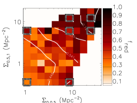
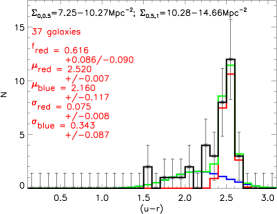
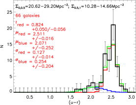
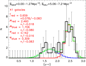
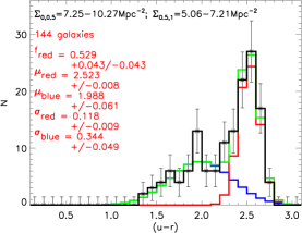
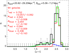
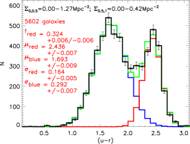
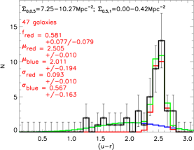
Figure 8: Example double gaussian fits to the colour distribution of $-20.5\leq\rm\,M_{r}\leq-20.0$ galaxies binned by density on scales $\rm\,\Sigma_{0,0.5}$ and $\rm\,\Sigma_{0.5,1}$. Top left: The density dependence of the red galaxy fraction, $\rm\,f_{red}$ for galaxies on scales $\rm\,\Sigma_{0,0.5}$ and $\rm\,\Sigma_{0.5,1}$, as the left-hand panel of Figure 9, except limited to galaxies in the $-20.5\leq\rm\,M_{r}\leq-20.0$ luminosity bin. Other panels: Fits to the $u-r$ colour distribution for galaxies in the bins indicated using black and white squares in the top-left panel. Panels refer to the bin in the equivalent position in the density-density plane. The colour distribution (points and black line) is in each case fit by a double-gaussian (green line) which is the combination of blue and red peaks (represented by blue and red lines). $\sqrt{(}N+2)$ errors are assigned to the counts in each bin of colour. The number of contributing galaxies and the derived parameters are also indicated in each panel.

We illustrate that the fits thus produced are sufficiently good in Figure 8. To do so we must select a single luminosity bin, $-20.5\leq\rm\,M_{r}\leq-20.0$. The top-left panel shows that the fraction of red galaxies, $\rm\,f_{red}$ can clearly be traced as a function of density computed on 0–0.5 $\rm\,Mpc$ vs 0.5–1 $\rm\,Mpc$ scales. To illustrate fitted populations at a variety of multiscale densities, and in particular including bins containing close to our minimum number of galaxies (25), we select the seven bins from this density-density plane as indicated by black and white squares. For each of these bins the full double gaussian fit to the $u-r$ colour distribution is shown in the other panels. Most importantly, both peaks can be seen in each panel, and the fits are as good as the data allows. For bins containing few galaxies, especially those with few blue (or red) galaxies, the fit parameters are uncertain. Whilst this is formally accounted for in fitting errors (see Section 4), errors on $\rm\,f_{red}$ are computed statistically sing the Gehrels (1986) approximation, combining Poissonian and Binomial statistical errors. For double gaussian fits to a large number of galaxies this approximates the fitting error, whilst for smaller numbers the statistical error is larger. However, the scatter between different, independent bins in the density-density plane provides the best estimate of the ”true” error: this is consistent with the statistical error, and is reduced once the three luminosity bins are coadded.

Kauffmann et al. (2004),Blanton et al. (2006) and Blanton & Berlind (2007) have all claimed that galaxy properties exhibit little dependence on density beyond $1\rm\,Mpc$. Beyond this separation, the correlation function of blue or red galaxies is consistent within $5\%$ of that expected if the type of galaxy only responds to its halo mass and halocentric position (Blanton & Berlind, 2007). Our choice of pairs of small and large scales, whose effects are to be compared (namely 0–0.5 $\rm\,Mpc$ vs 0.5–1, 0–1 vs 1–2, 0–2 vs 2–3), is designed to provide complimentary information. In each case we have selected an “interior” (circular) annulus and a larger scale annulus which meet but do not overlap. This provides independently measured quantities, but means that any signal on scales just beyond that measured by the small scale should be picked up on the large scale. To facilitate discussion of these scales, we introduce the division radius, $\rm\,r_{div}$ which is equal to 0.5, 1 and 2$\rm\,Mpc$ respectively for our three pairs of small and large scales. The $\rm\,\Sigma_{0,1}$ versus $\rm\,\Sigma_{1,2}$ plane examines the influence of $>1\rm\,Mpc$ scales. Smaller scales ($<0.5\rm\,Mpc$) trace local substructure. This is examined in the $\rm\,\Sigma_{0,0.5}$ versus $\rm\,\Sigma_{0.5,1}$ plane. Conversely, the $\rm\,\Sigma_{0,2}$ and $\rm\,\Sigma_{2,3}$ plane probes the largest scales measured. If galaxies only correlate with the properties of their embedding halo, then one might expect large scale density only to matter where those scales trace galaxies within the same halo (division radius, $\rm\,r_{div}\lesssim 2r_{200}$, a typical halo diameter). This occurs at $\rm\,M_{halo}\sim 2\times 10^{13}\rm\,M_{\odot}$ ($5\times 10^{12}\rm\,M_{\odot}$,$8\times 10^{13}\rm\,M_{\odot}$) for $\rm\,r_{div}=1\rm\,Mpc$ ($0.5\rm\,Mpc$,$2\rm\,Mpc$).

Figures 9, 10 and 11 examine how the relative fraction of red galaxies ($\rm\,\Delta(f_{red})$), the parameters describing the red peak ($\rm\,\Delta(\mu_{red})$, $\rm\,\Delta(\sigma_{red})$) and the blue peak ($\rm\,\Delta(\mu_{blue})$, $\rm\,\Delta(\sigma_{blue})$) depend upon small and large scale density for our selected planes of scale. Colour-coded bins in this plane are totally independent of each other. Overplotted contours are computed for a smoothed map of the data, using a gaussian smoothing kernel with $\sigma=1.5$pixels . Contours indicate the direction of change for each parameter in density-density space, and thus the importance of the two different scales. Smoothing reduces small scale noise, but note that local or abrupt features can be smoothed away.

       

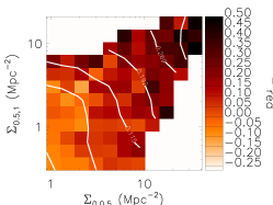
Figure 9: The density dependence of the red galaxy fraction, $\rm\,\Delta(f_{red})$, for $\-21.5<\rm\,M_{r}<-20.0$ galaxies binned in two scales of density. Left: on scales $\rm\,\Sigma_{0,0.5}$ and $\rm\,\Sigma_{0.5,1}$; Centre: on scales $\rm\,\Sigma_{0,1}$ and $\rm\,\Sigma_{1,2}$; Right: on scales $\rm\,\Sigma_{0,2}$ and $\rm\,\Sigma_{2,3}$. Almost vertical contours illustrate that $\rm\,\Delta(f_{red})$ depends mostly on small scale density.

       

       

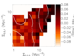
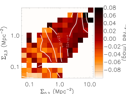
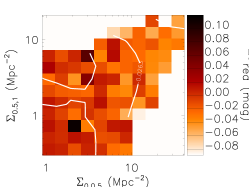
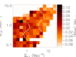
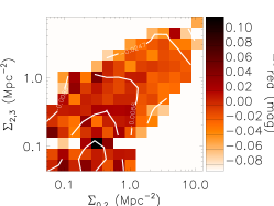
Figure 10: The density dependence of the red peak parameters $\rm\,\mu_{red}$ (above) and $\rm\,\sigma_{red}$ (below), for $\-21.5<\rm\,M_{r}<-20.0$ galaxies binned in two scales of density. Left: on scales $\rm\,\Sigma_{0,0.5}$ and $\rm\,\Sigma_{0.5,1}$; Centre: on scales $\rm\,\Sigma_{0,1}$ and $\rm\,\Sigma_{1,2}$; Right: on scales $\rm\,\Sigma_{0,2}$ and $\rm\,\Sigma_{2,3}$.

       

       

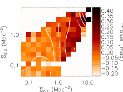
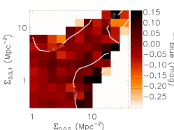
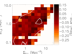
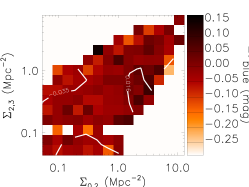
Figure 11: The density dependence of the blue peak parameters $\rm\,\mu_{blue}$ (above) and $\rm\,\sigma_{blue}$ (below), for $\-21.5<\rm\,M_{r}<-20.0$ galaxies binned in two scales of density. Left: on scales $\rm\,\Sigma_{0,0.5}$ and $\rm\,\Sigma_{0.5,1}$; Centre: on scales $\rm\,\Sigma_{0,1}$ and $\rm\,\Sigma_{1,2}$; Right: on scales $\rm\,\Sigma_{0,2}$ and $\rm\,\Sigma_{2,3}$.

We also quantify the significance of any dependence on large scale density, at fixed small scale density. For each parameter and set of scales, we compute the Spearman Rank Correlation Coefficient ($\rho$) of the correlation with large scale density, and the probability, $\rm\,P_{L}$, of attaining the value of $\rho$ given a null hypothesis in which the parameter depends only upon small scale density. The method used to compute $\rm\,P_{L}$ is described in Appendix B. A value of $\rm\,P_{L}=0.5$ means no significance, while $\rm\,P_{L}=0$ is a high significance anti-correlation and $\rm\,P_{L}=1$ is a high significance positive correlation . Subsections of the small scale density range are also tested so that effects of large scale density can be detected which are local in density space. The results are recorded in Table 1.

Table 1: For different choices of small and large scale density and a given range of small scale density (columns 1 and 2, units $\rm\,Mpc^{-2}$), we provide the Spearman Rank Correlation Coeffiecient $\rho$ which measures the correlation between each parameter and the large scale density (columns 3 to 7). $\rm\,P_{L}$, the probability that this coefficient is greater than would be expected in the absence of any intrinsic large scale correlation (i.e. any remaining correlation is purely a result of correlations between the parameter and small scale density, and between density on the two scales) is provided in columns 8 to 12. Computed using a monte-carlo technique, a value of $\rm\,P_{L}=1$ implies a highly significant positive correlation; $\rm\,P_{L}=0$ implies a highly significant negative correlation and $\rm\,P_{L}=0.5$ implies no correlation.

small scale	large scale	$\rho$($\rm\,\mu_{red}$)	$\rho$($\rm\,\mu_{blue}$)	$\rho$($\rm\,\sigma_{red}$)	$\rho$($\rm\,\sigma_{blue}$)	$\rho$($\rm\,f_{red}$)	$\rm\,P_{L}$($\rm\,\mu_{red}$)	$\rm\,P_{L}$($\rm\,\mu_{blue}$)	$\rm\,P_{L}$($\rm\,\sigma_{red}$)	$\rm\,P_{L}$($\rm\,\sigma_{blue}$)	$\rm\,P_{L}$($\rm\,f_{red}$)
$\rm\,\Sigma_{0,0.5}$	$\rm\,\Sigma_{0.5,1}$	0.4444	0.5008	-0.3799	-0.2157	0.6308	0.8210	0.9960	0.2850	0.0800	1.0000
$0-2$		0.4236	0.6096	-0.3112	-0.0276	0.4751	0.9933	1.0000	0.1387	0.7507	0.9770
$1-10$		0.2527	0.4038	-0.1888	-0.1117	0.4645	0.9453	0.9990	0.3020	0.1937	1.0000
$2-10$		0.1940	0.3806	-0.1627	-0.2279	0.4420	0.8073	0.9953	0.2860	0.0657	0.9947
$2-30$		0.4083	0.4581	-0.3538	-0.3057	0.6232	0.5663	0.9750	0.2983	0.0353	0.9960
$4-30$		0.3598	0.3767	-0.3619	-0.3675	0.5894	0.4470	0.9160	0.2193	0.0280	0.9773
$\rm\,\Sigma_{0,1}$	$\rm\,\Sigma_{1,2}$	0.3166	0.5819	-0.3642	0.0515	0.4190	0.1020	0.9910	0.4430	0.3257	0.5287
$0-2$		0.1097	0.4768	-0.1227	0.0008	0.1581	0.4170	0.9997	0.5893	0.1837	0.8313
$1-10$		0.0381	0.4238	-0.2040	0.0857	0.2067	0.0167	0.8117	0.5710	0.3850	0.2853
$2-10$		0.0440	0.3318	-0.2322	0.2158	-0.0619	0.1313	0.7177	0.2760	0.7947	0.0273
$2-30$		0.2206	0.3858	-0.3392	0.0607	0.1786	0.2073	0.7137	0.2763	0.7840	0.0337
$4-30$		0.1754	0.3537	-0.2074	0.0456	0.0231	0.3583	0.7917	0.6233	0.7767	0.0337
$\rm\,\Sigma_{0,2}$	$\rm\,\Sigma_{2,3}$	0.4951	0.5785	-0.4314	0.1280	0.3713	0.8030	0.9487	0.0370	0.5063	0.0503
$0-2$		0.3860	0.4945	-0.3618	0.1099	0.1262	0.9280	0.9900	0.0170	0.4307	0.0937
$1-10$		0.0990	0.2664	-0.2232	-0.2282	0.1356	0.0177	0.1920	0.7230	0.0727	0.0063
$2-10$		1524	0.0527	-0.0809	-0.2761	-0.1869	0.0100	0.1393	0.8033	0.1837	0.0000

A common feature of all the panels in Fig. 9, 10 and 11 is that contours, where they exist, are more closely aligned with the large scale axis than with the small scale one, indicating that the parameters react more strongly to smaller scales (even $<0.5\rm\,Mpc$) than to the larger ones.

Nonetheless, there is a highly significant positive correlation of $\rm\,\Delta(f_{red})$ with $\rm\,\Sigma_{0.5,1}$, at fixed $\rm\,\Sigma_{0,0.5}$. This must reflect a transformation process for galaxies which relates to the environment and is imprinted on scales beyond $0.5\rm\,Mpc$. However parameters defining the red peak ($\rm\,\Delta(\mu_{red})$ and $\rm\,\Delta(\sigma_{red})$) show no significant trend with $\rm\,\Sigma_{0.5,1}$ at fixed $\rm\,\Sigma_{0,0.5}$, other than $\rm\,\Delta(\mu_{red})$ at low density ($\rm\,\Sigma_{0,0.5}=0-2\rm\,Mpc^{-2}$). A significant residual positive correlation does exist for the blue peak position $\rm\,\Delta(\mu_{blue})$ with $\rm\,\Sigma_{0.5,1}$, though this is weaker than the trend with $\rm\,\Delta(f_{red})$.

On $>1.0\rm\,Mpc$ scales there is no significant correlation of $\rm\,\Delta(f_{red})$ with $\rm\,\Sigma_{1,2}$ at fixed $\rm\,\Sigma_{0,1}$ other than a $\sim 2\sigma$ level anti-correlation at low density ($\rm\,\Sigma_{0,1}=2-10\rm\,Mpc^{-2}$). A stronger anti-correlation exists between the position of the red peak $\rm\,\Delta(\mu_{red})$ and $\rm\,\Sigma_{1,2}$ at intermediate density ($\rm\,\Sigma_{0,1}=1-10\rm\,Mpc^{-2}$). The blue peak position $\rm\,\Delta(\mu_{blue})$ does correlate positively with $\rm\,\Sigma_{1,2}$, though this is only significant at low density ($\rm\,\Sigma_{0,1}=0-2\rm\,Mpc^{-2}$). The lack of any positive correlation with densities above $1\rm\,Mpc$ scales, at least for $\rm\,\Delta(f_{red})$ and $\rm\,\Delta(\mu_{red})$, and at higher densities typical of groups and clusters, indicates that there is no longer any direct impact of these environments on these galaxy properties. This is consistent with the results of Kauffmann et al. (2004), Blanton et al. (2006) and Blanton & Berlind (2007). The anti-correlations are interesting however, and deserve further attention.

At $>2\rm\,Mpc$ scales and at intermediate density ($\rm\,\Sigma_{0,2}=2-10\rm\,Mpc^{-2}$), the anti-correlation of $\rm\,\Delta(f_{red})$ with $\rm\,\Sigma_{2,3}$ is even more significant. For roughly the same range of density ($\rm\,\Sigma_{0,2}=1-10\rm\,Mpc^{-2}$) we also see a highly significant anti-correlation of $\rm\,\Delta(\mu_{red})$ with $\rm\,\Sigma_{2,3}$. In other words, red galaxies which have intermediate to large $0-2\rm\,Mpc$ scale densities avoid regions overdense on $2-3\rm\,Mpc$ scales, and are otherwise bluer on average. Blue galaxies, on the other hand, exhibit a positive correlation of $\rm\,\Delta(\mu_{blue})$ with $\rm\,\Sigma_{2,3}$, but only at low density ($\rm\,\Sigma_{0,2}=0-2\rm\,Mpc^{-2}$), as seen on $1-2\rm\,Mpc$ scales. The width of the red peak $\rm\,\Delta(\sigma_{red})$ is also anti-correlated (in this case the same direction as the trend with small scale density) with $\rm\,\Sigma_{2,3}$ at these densities.

5.2.1 Summary of observational results:

To summarize the way in which the galaxy colour distribution traces density on different scales:

• The fraction of red galaxies $\rm\,f_{red}$ increases dramatically with increasing local ($<0.5\rm\,Mpc$ scale) density. The properties of both peaks also change: the red peak becomes redder and narrower, and the blue peak becomes redder and broader.

• The position and width of the red peak, $\rm\,\mu_{red}$ and $\rm\,\sigma_{red}$ show no residual dependence on $0.5-1.0\rm\,Mpc$ scales.

• The fraction of red galaxies and the position of the blue peak, $\rm\,f_{red}$ and $\rm\,\mu_{blue}$, both show residual positive correlation with density on $0.5-1.0\rm\,Mpc$ scales. Other than some dependence of $\rm\,\mu_{blue}$ at very low densities, there are no significant positive correlations with densities computed on $>1.0\rm\,Mpc$ scales.

• Nonetheless, at fixed smaller scales, there exist significant anti-correlations with large scale density ($\rm\,f_{red}$ and $\rm\,\mu_{red}$ with $\rm\,\Sigma_{1,2}$, $\rm\,\Sigma_{2,3}$), typically at intermediate values of interior density.

• Correlations with larger scale density exist at low values of small scale density ($\rm\,\mu_{red}$ with $\rm\,\Sigma_{0.5,1}$ at low $\rm\,\Sigma_{0,0.5}$, $\rm\,\sigma_{red}$ with $\rm\,\Sigma_{2,3}$ at low $\rm\,\Sigma_{0,2}$, $\rm\,\mu_{blue}$ with $\rm\,\Sigma_{0.5,1}$, $\rm\,\Sigma_{1,2}$, $\rm\,\Sigma_{2,3}$ at low $\rm\,\Sigma_{0,0.5}$, $\rm\,\Sigma_{0,1}$, $\rm\,\Sigma_{0,2}$ respectively). This suggests that relatively isolated galaxies react in some ways to their environments on large scales. However this result might be explained by the effects of correlated noise on density measurements. We discuss this effect in Appendix A.

6 Multiscale density dependences in the halo model framework

6.1 Dependence of halo properties on density

To aid our interpretation of these results, we cross-correlate the sample with the groups catalogue of Yang et al. (2007, Y07) to examine how halo mass and group-centric radius depend upon our density measurements at different scales. We emphasize that our approach has been to compute an entirely model-independent, measurable quantity (density) and that this exercise thus serves as an examination of the halo model in an independent parameter space.

The Y07 catalogue is constructed from the SDSS Data Release 4 (DR4) catalogue (via the New York University Value Added Galaxy Catalogue, NYU-VAGC, Blanton et al., 2005), incomplete for our sample. A friends-of-friends algorithm is applied to the survey for group detection, and the total luminosity, $L_{19.5}$, of galaxies is computed for each group down to an $r$-band magnitude of $M_{r,0.1\mathrm{ev}}=-19.5$ (note that in Y07 all luminosities are k- and evolution-corrected to $z=0.1$). A halo mass is assigned to each group assuming a one to one relation in rank order of halo mass with $L_{19.5}$. This is in turn used to redefine group membership, which is iterated until a stable solution is found. A halo is defined so long as a member galaxy with $M_{r,0.1\mathrm{ev}}<-19.5$ makes it into the sample. At the upper redshift boundary of our sample $z=0.08$, this limit ensures that the group catalog is complete to $\log_{10}(\rm\,M_{\mathrm{halo}}/\rm\,M_{\odot})=11.6$ and includes all galaxies with $\rm\,M_{r}<-20.434$ (mag as defined in Section 2, corrected to $z=0$ rest-frame, no evolution correction). This sample, after removal of galaxies due to DR4 edge effects for which $\rm\,M_{halo}$ could not be estimated, numbers 38733 galaxies. Importantly, this catalogue provides halo masses for individual galaxies, as well as groups with more than one known member.

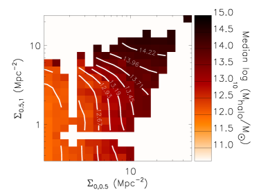
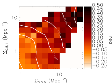
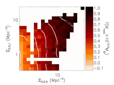
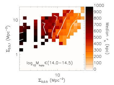
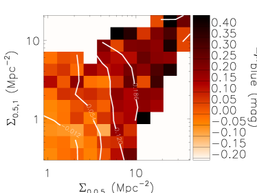
Figure 12: A comparison between the dependence of halo mass and halo-centric radius with density on scales $\rm\,\Sigma_{0,0.5}$ and $\rm\,\Sigma_{0.5,1}$ (left) and the dependence of the colour distribution parameters $\rm\,f_{red}$, $\rm\,\mu_{blue}$ and $\rm\,\mu_{red}$ on $\rm\,\Sigma_{0,0.5}$ and $\rm\,\Sigma_{0.5,1}$ (right). The top, centre and lower panels on the left illustrate the behaviour of the median halo mass, the fraction of galaxies inside haloes $>10^{12.5}\rm\,M_{\odot}$, and the median halo-centric radius in haloes of $10^{14.0-14.5}\rm\,M_{\odot}$, taken from the Y07 catalogue.

Figures 12, 13 and 14 illustrate how the halo masses $\rm\,M_{halo}$ and halo-centric radii $\rm\,r_{h}$ correlate with density computed in our three choices of small versus large scale density plane ($\rm\,r_{div}=0.5$,$1$,$2\rm\,Mpc$). The left panels illustrate (from top to bottom) the dependence on density of the median halo mass, the fraction of galaxies in haloes of $>10^{12.5}\rm\,M_{\odot}$ (both restricted to grid pixels with $\geq 25$ galaxies), and the median halo-centric radius for galaxies in massive $10^{14-14.5}\rm\,M_{\odot}$ haloes (for $\geq 5$ galaxies). Each panel is also overplotted with contours, computed for a grid smoothed in exactly the same way as those in Figures 9 to 11.

For direct visual comparison, the right hand panels reproduce the equivalent dependence of $\rm\,\Delta(f_{red})$, $\rm\,\Delta(\mu_{red})$ and $\rm\,\Delta(\mu_{blue})$ on density, as already seen in Figures 9 to 11.

The median halo mass and the fraction of galaxies in $>10^{12.5}\rm\,M_{\odot}$ haloes both depend mostly on the smallest scale densities. In more massive haloes the halo diameter exceeds $\rm\,r_{div}=0.5\rm\,Mpc$ ($2r_{200}\sim 0.4\rm\,Mpc$ for $10^{12.5}\rm\,M_{\odot}$ haloes) and thus $\rm\,\Sigma_{0.5,1}$ becomes more important, particularly at higher density where more massive haloes dominate. On $\rm\,\Sigma_{0,1}$ versus $\rm\,\Sigma_{1,2}$ scales ($\rm\,r_{div}=1\rm\,Mpc$), the contours are closer to vertical, and on $\rm\,\Sigma_{0,2}$ versus $\rm\,\Sigma_{2,3}$ scales ($\rm\,r_{div}=2\rm\,Mpc$) both parameters anti-correlate with $\rm\,\Sigma_{2,3}$ at fixed $\rm\,\Sigma_{0,2}$. This results mainly from the way halo centric radius $\rm\,r_{h}$ tracks density on different scales. For $10^{14-14.5}\rm\,M_{\odot}$ haloes the contours tracking the change in $\rm\,r_{h}$ with density are almost vertical with $\rm\,r_{div}=0.5\rm\,Mpc$, but moving to larger scales become diagonal for $\rm\,r_{div}=1\rm\,Mpc$ (larger median radius at smaller $\rm\,\Sigma_{0,1}$ but larger $\rm\,\Sigma_{1,2}$), and almost horizontal with $\rm\,r_{div}=2\rm\,Mpc$ (radius positively correlates with $\rm\,\Sigma_{2,3}$). The reason for this is fairly obvious: a galaxy at the centre of its halo will have high densities within annuli up to the size of the halo ($r_{200}\sim 1.1$,$2.5\rm\,Mpc$ for $\rm\,M_{halo}=10^{14}$,$10^{14.5}\rm\,M_{\odot}$) and low densities on larger scales. A galaxy in the outskirts of this halo will experience the opposite, since the dense halo core is located within the larger scale annulus. Moving to smaller halo masses than $10^{14-14.5}\rm\,M_{\odot}$, this pattern simply shifts to smaller scales.

At the point of accretion, a galaxy moves from the infalling halo (low $\rm\,M_{halo}$), to the more massive halo (high $\rm\,M_{halo}$ and high $\rm\,r_{h}$), but the change in density will not be instantaneous. Therefore at high density on large scales there are not only more galaxies with large $\rm\,r_{h}$ within the massive halo, but also more galaxies assigned instead to an infalling halo of lower mass. This can account for the anti-correlations of both median halo mass and the fraction of galaxies in $>10^{12.5}\rm\,M_{\odot}$ haloes with large scale density.

This effect is further amplified by the depth of the cylinder, required to account for redshift-space distortions (the “finger of God effect”). By integrating to $\pm 1000\rm\,km\,s^{-1}$ along the line of sight, the contribution of galaxies from outside a massive halo is increased, including galaxies from the fore- and background.

6.2 Comparison with the dependence of galaxy properties on density

Now we make a qualitative comparison of the density dependence of galaxy properties with the density dependence of the assumed embedding halo to examine whether and how the halo model can explain the way the colour distribution of galaxies traces density on different scales.

Both $\rm\,M_{halo}$ and $\rm\,r_{h}$ trace mostly $<0.5\rm\,Mpc$ scales in the $\rm\,\Sigma_{0,0.5}$ versus $\rm\,\Sigma_{0.5,1}$ plane. Therefore any such dependence of galaxy properties can be explained by invoking either trends with halo mass or halo-centric radius. On larger scales (larger $\rm\,r_{div}$) this is no longer the case. The primary dependence on small scales (contours close to vertical) of $\rm\,\Delta(f_{red})$, $\rm\,\Delta(\mu_{red})$ and $\rm\,\Delta(\mu_{blue})$ more closely resemble trends with halo mass than with radius.

Indeed $\rm\,\Delta(f_{red})$ trends in particular are very well matched qualitatively to the trends seen for the fraction of galaxies in $>10^{12.5}\rm\,M_{\odot}$ haloes, including the roughly equal spacing of contours. Trends on all scales are very comparable, but the anti-correlation with $\rm\,\Sigma_{2,3}$ at fixed $\rm\,\Sigma_{0,2}$ is particularly striking. The anti-correlation for haloes traces the accretion of galaxies onto the halo in the infall regions, and the reproduction of this trend for the fraction of red galaxies is intriguing. It provides strong circumstantial evidence that galaxies remain blue until they have experienced some truncation mechanism which is intimitely linked to the accretion time onto a massive halo. This is fully consistent with a simple model in which galaxies become red at some interval after their incorporation into a halo of mass $\gtrsim 10^{12-13}\rm\,M_{\odot}$, which can also match total red fractions as a function of halo mass and redshift (McGee et al., 2009). However the qualitative dependence on density is not strongly sensitive to the choice of limiting halo mass: similar looking trends are produced with limits in the range $\sim 10^{12.5-13.5}\rm\,M_{\odot}$, with contours becoming slightly more horizontal with larger limiting mass.

$\rm\,\mu_{red}$ does not trace density on $>0.5\rm\,Mpc$ scales in the same way as the median halo mass or the fraction of galaxies in haloes above a given threshold. Instead the positive correlations with density are all on local $<0.5\rm\,Mpc$ scales, and $\rm\,\mu_{red}$ anti-correlates with density on $1.0-2.0\rm\,Mpc$ scales. The lack of positive density dependence scales greater than $0.5\rm\,Mpc$ can be related to subhalo or radial effects, in that the colour may be imprinted at a time when the galaxy’s $<0.5\rm\,Mpc$ scale subhalo was not part of the current $>0.5\rm\,Mpc$ scale main halo. Alternatively, if the colour of red galaxies is influenced by some combination of halo mass and halo-centric radius such that in massive haloes galaxies with larger $\rm\,r_{h}$ are likely to be bluer than those in the centre, then it is also possible to qualitatively reproduce the observed trends.

The colour of a red (assuming passive) galaxy can be driven by either age (luminosity weighted time since stars were formed), or metallicity of the stars. If age is the driving factor then the subhalo hypothesis is hard to reconcile with observations: i.e. If galaxies all became red within such small subhaloes then we cannot explain the trend of $\rm\,f_{red}$ with $>0.5\rm\,Mpc$ scale density. Halo-centric radius, on the other hand, should correlate with the time since a galaxy was accreted onto the halo, and provides a possible solution. If metallicity is the driving factor, the galaxy’s environment at the time it was forming stars should be more important: i.e. the subhalo. Thus we suggest that where $\rm\,\mu_{red}$ is concerned, the relative importance of halo-centric radius versus local density is equivalent to the relative importance of age versus metallicity. The anti-correlation of $\rm\,\mu_{red}$ with density on $1-2\rm\,Mpc$ scales suggests that the average colour of red galaxies is bluer outside more massive haloes ($\gtrsim 2\times 10^{13}\rm\,M_{\odot}$). This is consistent with both hypotheses (red galaxies belonging to smaller infalling haloes are younger and metal poorer).

We note that these trends describe only the influence of environment on red galaxies in the luminosity range $-21.5\leq\rm\,M_{r}\leq-20.0$, and that the way in which both age and metallicity depend upon their halo mass seems to be a function of stellar mass (Pasquali et al., 2010). Indeed, the local density of red sequence galaxies correlates with both age and metallicity, even at fixed luminosity and colour (Cooper et al., 2010), whilst there is no clear correlation with larger scale (6Mpc) density (Thomas et al., 2010, who also show thec contribution of rejuvenated galaxies decreases with density). Thus this complex picture has to be taken with the caveat that not all red galaxies are passive, and not all passive red galaxies have comparible star formation histories.

The blue peak colour $\rm\,\mu_{blue}$ depends on $0-1\rm\,Mpc$ scale densities in the same way as $\rm\,f_{red}$, and therefore a pure halo mass dependence can be similarly invoked. $\rm\,\mu_{blue}$ probably traces the level of recent star formation in a typical star forming galaxy, and so this means that such galaxies experience partial truncation of their fuel supplies inside massive haloes, consistent with observations of truncated gas disks or anemic spirals in the Virgo cluster (e.g. Giovanelli & Haynes, 1985; Koopmann & Kenney, 2004; Gavazzi et al., 2006; Chung et al., 2009, and references therein).It is currently unclear whether this is necessarily a step on the path to total truncation and transition to a red colour.

$\rm\,\mu_{blue}$ exhibits residual large scale dependence at low values of small scale density, no matter which radius $\rm\,r_{div}$ is chosen to separate small from large scales. This dependence cannot be pure halo mass dependence, because the median halo mass has such residual dependence on large scale only if $\rm\,r_{div}=0.5\rm\,Mpc$. This might merely be a result of correlated noise in the density plane (see Appendex A), but there is no reason this should apply to certain parameters and not others. Otherwise the suggestion is that relatively isolated blue galaxies are redder when they live in relatively overdense larger scale environments. On such scales (including $>2.0\rm\,Mpc$) this might relate to an earlier formation time of a galaxy living in a large scale overdensity coupled with a declining star formation history, or to a more efficient cooling of hot gas onto galaxies in more isolated environments.

   

   

   

   

   

   

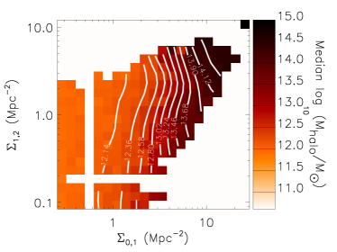
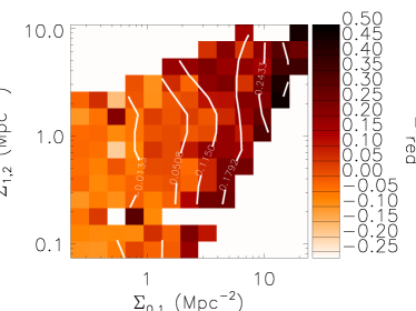
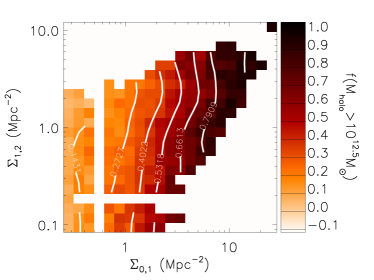
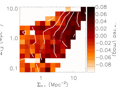
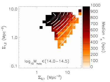
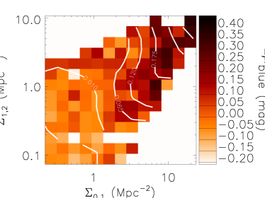
Figure 13: As Figure 12, but on density scales $\rm\,\Sigma_{0,1}$ and $\rm\,\Sigma_{1,2}$.

   

   

   

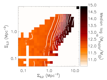
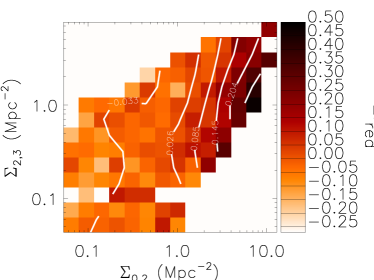
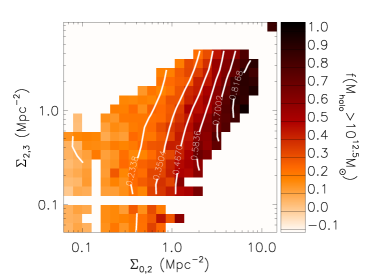
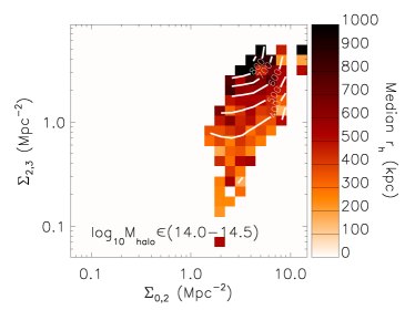
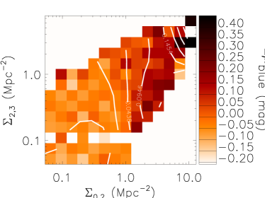
Figure 14: As Figure 12, but on density scales $\rm\,\Sigma_{0,2}$ and $\rm\,\Sigma_{2,3}$.

We conclude that the halo model can provide an excellent qualitative description of the dependence of the parameters governing the galaxy colour distribution, in particular $\rm\,f_{red}$, $\rm\,\mu_{red}$ and $\rm\,\mu_{blue}$, on simple annular density measurements on a range of scales from $0-3\rm\,Mpc$. The data is consistent with a simple picture in which the density dependence of the fraction of red galaxies $\rm\,f_{red}$ and the peak colour of blue galaxies $\rm\,\mu_{blue}$ is governed mainly by the fraction of galaxies assigned to haloes above some threshold halo mass ($10^{12.5}\rm\,M_{\odot}$ provides a reasonable but not unique description in this case). This suggests that the gas supply regulating star formation can be partially or completely suppressed as a function of halo mass. The halo model is particularly good at explaining the anti-correlation of $\rm\,f_{red}$ with large scale density. This can be explained if galaxies not yet or recently incorporated into a relatively massive halo have not experienced the blue to red transition. The lack of positive correlations with density beyond $0.5\rm\,Mpc$ suggests that the red peak colour $\rm\,\mu_{red}$ traces only local density within subhaloes (explicable if $\rm\,\mu_{red}$ traces metallicity) or with additional dependence on halo-centric radius (since if suppression time is linked to the time a galaxy was accreted onto a halo, and this is correlated with radius, then a red galaxy will be older and thus also redder towards the halo centres).

7 Conclusions

We have developed a new multiscale method to characterize the dependence of galaxy properties on environment. This provides a model-independent, rich parameter space in which to evaluate galaxy properties.

In this paper we have examined the dependence of the $u-r$ colour distribution for galaxies in the luminosity range $-21.5\leq\rm\,M_{r}\leq-20$ on multiscale density. This is parameterized using the double gaussian model, with parameters $\rm\,f_{red}$ (the fraction of red galaxies), $\rm\,\mu_{red}$ and $\rm\,\sigma_{red}$ (the position and width of the red peak) and $\rm\,\mu_{blue}$ and $\rm\,\sigma_{blue}$ (the position and width of the blue peak).

We confirm and extend known trends with small scale ($\lesssim 0.5-1\rm\,Mpc$) density:

• Galaxies in denser environments are more likely to be red ($\rm\,f_{red}$), implying an almost complete truncation of star formation.

• If they are still blue (star forming), then they are also likely to be relatively redder in denser environments ($\rm\,\mu_{blue}$) although with greater scatter ($\rm\,\sigma_{blue}$), implying partial but varied truncation of gas supplies, possibly relating to truncated gas disks such as those observed in the Virgo cluster.

• Red Galaxies are redder ($\rm\,\mu_{red}$) and with less scatter ($\rm\,\sigma_{red}$) in denser environments. This implies that they either form earlier and/or are more metal-rich, and that this formation path is also less varied than galaxies in less dense environments. This depends upon the environment of a galaxy during its epoch of star formation.

On larger scales:

• No parameter correlates positively and significantly with density on scales $>1\rm\,Mpc$, excluding trends seen for relatively isolated galaxies where correlated noise in the measurement of density might be important. This confirms the results of Kauffmann et al. (2004), Blanton et al. (2006) and Blanton & Berlind (2007).

• Although all parameters correlate most strongly with density on $<0.5\rm\,Mpc$ scales, a residual positive correlation of $\rm\,f_{red}$ and $\rm\,\mu_{blue}$ with $0.5-1\rm\,Mpc$ scale density at fixed smaller scale density implies that total or partial truncation of star formation can relate to a galaxy’s environment on these scales. A $1\rm\,Mpc$ diameter halo corresponds to a mass of $\sim 2\times 10^{13}\rm\,M_{\odot}$ and a typical crossing time on the order of $4\rm\,Gyr$, and one or both of these parameters must relate to a truncation mechanism which is active on these scales.

• On $>2\rm\,Mpc$ scales $\rm\,f_{red}$ anti-correlates with density at fixed smaller scale density, and $\rm\,\mu_{red}$ anti-correlates with density on $>1\rm\,Mpc$ scales. In other words galaxies are more likely to have ongoing star formation, or if not then to be relatively blue, when the large scale density is relatively high for the density on smaller scales (they live at projected distances $\sim 1-3\rm\,Mpc$ from a local overdensity).

We interpret these trends qualitatively using the halo model. To make this comparison we utilize the halo catalogue of Y07 which is constructed using a friends of friends group finder, and under the assumptions that galaxies live in haloes, and that the mass of these haloes has a one to one relationship with the total galaxy light. The properties of embedding haloes has been cross-correlated with our galaxy catalogue to examine how halo properties trace multiscale density. By comparing this dependence to that of galaxy colours, we find:

• Qualitatively, the multiscale dependence of $\rm\,f_{red}$ and $\rm\,\mu_{blue}$ is remarkably comparable to that seen in the fraction of galaxies living in haloes above a given threshold mass in the range $\sim 10^{12.5-13.5}\rm\,M_{\odot}$. This is consistent with a scenario in which galaxies can experience truncation of their star formation at some time after they are accreted onto a halo.

• The halo model offers a simple and yet profound explanation for anti-correlations with larger (particularly $>2\rm\,Mpc$) scale density. For galaxies at large radial distances from the centre of massive haloes the halo core is included in measurements of density on large scales. Thus this region of parameter space traces the accretion region of haloes (effectively marking the crossover from the one to the two halo term in the correlation function). Anti-correlations on these scales therefore trace the accretion region of haloes. That many such galaxies are still blue implies that the influence of environment is felt at or after accretion onto a massive halo.

• $\rm\,\mu_{red}$ correlates positively with density only on $<0.5\rm\,Mpc$ scales, implying that the red colour is set by physics within subhaloes of this size. In this case we suggest metallicity effects must drive these trends, since we know that age must correlate with larger scale densities: i.e. galaxies become red due to the influence of $0.5-1\rm\,Mpc$ scales ($\rm\,f_{red}$ correlates positively with $\rm\,\Sigma_{0.5,1}$). However we cannot rule out age effects if the $0.5-1\rm\,Mpc$ scale dependence of $\rm\,\mu_{red}$ is negated due to a combination of halo mass and radial trends.

Whilst we have restricted ourselves in this paper to qualitative comparisons within the context of the halo model, we advocate the use of multiscale density to quantitatively examine physically motivated models (from simple halo occupation models to semi-analytically populated haloes). This provides a uniquely rich and observationally motivated parameter space to examine the dependence of galaxy properties on environment.

Appendix A Poisson sampled neighbours in a correlated density field

The number of neighbours brighter than a given luminosity limit, and within $1000~{}\rm\,km\,s^{-1}$ of a given galaxy, is clearly not going to provide the perfect measure of its environment, either in the sense of “that which best correlates with the galaxy’s properties” or in the sense of “that which traces the underlying dark matter density field”. In most senses this is unimportant: it merely provides a measurable tracer of environment at the position of each galaxy and is the best that we can do empirically, without assuming a halo model.

Blanton et al. (2006) has suggested that a Poisson-sampled galaxy field can lead to correlated noise in the small versus large scale density plane and therein to false correlations with large scale density. Effectively, sampling of rare, quantized tracers such as bright galaxies leads to large errors sampled from a Poisson distribution, particularly on the smallest scales and the lowest densities where these errors are largest. Assuming some perfect, underlying measure of environment exists, measurements with large errors might have residuals which correlates with the large scale density measurement, which has a higher signal to noise. In reality this is highly complex, relating to our observing galaxies at random positions along their orbits; projection effects; the correlated measurements of density for neighbouring galaxies and the less than $100\%$ deterministic nature of galaxy formation which allows a galaxy to enter our luminosity selected sample. Modelling all these effects and their influence on the error vector in our density planes is well beyond the scope of this paper.

Nonetheless, we do not believe that correlated noise significantly influences the departure from vertical contours, since we do have some plots with contours which appear almost vertical at all densities, as confirmed using the statistical test outlined in Appendix B. If correlated noise has any influence, it is most likely at small density, where $N/\sqrt{(}N)$ is smaller, and thus we shall treat any possible influence of large scales at small density with caution.

Appendix B Significance of parameter dependence on Large Scales

To test the significance of residual large scale dependencies, we setup a null hypothesis: that only smaller scale density matters. Under this assumption, the predicted influence of large scale density can be tested using bootstrap catalogues, resampled from the real one as follows: The galaxies in each bin of luminosity are ranked in order of their smaller scale density. For every galaxy in the sample, one of the twenty nearest in rank is selected to replace it, regardless of its large scale density. This effectively shuffles the large scale information whilst preserving the small scales (imposing vertical contours in the small versus large scale density plane). The usual fitting analysis is applied to the resulting bootstrap catalogue, and the residual parameter set ($\rm\,\Delta(f_{red})$, $\rm\,\Delta(\mu_{red})$, $\rm\,\Delta(\sigma_{red})$, $\rm\,\Delta(\mu_{blue})$, $\rm\,\Delta(\sigma_{blue})$) is computed at each point in the 2D density grid. Three thousand such catalogues are created, resulting in three thousand such parameter sets for comparison with the true parameter set.

The Spearman Rank Correlation Coefficient, $\rho$ (Spearman, 1904) tests the strength of correlation between the rank of one variable and another, and therefore does not assume a linear correlation between the parameters themselves. Computing this coefficient for the correlation between each derived parameter and the large scale density for all bootstrap catalogues defines the expected distribution of $\rho$ in the case that the null hypothesis were true (i.e. no large scale dependence). Therefore the significance that additional dependence on large scales exists (on top of that induced by correlations with small scale density, averaged over the whole 2D density grid) can be quantified as the frequency of coefficients determined from the set of bootstrap catalogues which are more extreme than that computed for the real data. We define $\rm\,P_{L}$ as the fraction of bootstrap samples for which the real data coefficient is greater than the bootstrap one. A value of $\rm\,P_{L}$ close to one infers additional positive correlation on large scales, whilst values close to zero infer additional negative correlation.

References

- Adelman-McCarthy et al. (2007) Adelman-McCarthy, J. K., et al., 2007, ApJS, 172, 634
- Baldry et al. (2006) Baldry, I. K., Balogh, M. L., Bower, R. G., Glazebrook, K., Nichol, R. C., Bamford, S. P., & Budavari, T. 2006, MNRAS, 373, 469
- Baldry et al. (2004) Baldry, I. K., Glazebrook, K., Brinkmann, J., Ivezić, Ž., Lupton, R. H., Nichol, R. C., & Szalay, A. S. 2004, ApJ, 600, 681
- Balogh et al. (2004a) Balogh, M., Eke, V., Miller, C., Lewis, I., Bower, R., Couch, W., Nichol, R., et al., 2004a, MNRAS, 348, 1355
- Balogh et al. (2004b) Balogh, M. L., Baldry, I. K., Nichol, R., Miller, C., Bower, R., & Glazebrook, K. 2004b, ApJL, 615, L101
- Berlind et al. (2003) Berlind, A. A., Weinberg, D. H., Benson, A. J., et al., 2003, ApJ, 593, 1
- Blanton & Berlind (2007) Blanton, M. R. & Berlind, A. A. 2007, ApJ, 664, 791
- Blanton et al. (2006) Blanton, M. R., Eisenstein, D., Hogg, D. W., & Zehavi, I. 2006, ApJ, 645, 977
- Blanton & Roweis (2007) Blanton, M. R. & Roweis, S. 2007, AJ, 133, 734
- Blanton et al. (2005) Blanton, M. R., Schlegel, D. J., Strauss, M. A., et al, 2005, AJ, 129, 2562
- Budavári (2009) Budavári, T. 2009, PASP, in press
- Budavári et al. (2003) Budavári, T., Connolly, A. J., Szalay, A. S., Szapudi, I., Csabai, I., Scranton, R., et al., 2003, ApJ, 595, 59
- Budavári et al. (2007) Budavári, T., Dobos, L., Szalay, A. S., Greene, G., Gray, J., & Rots, A. H. 2007, in Astronomical Society of the Pacific Conference Series, Vol. 376, Astronomical Data Analysis Software and Systems XVI, ed. R. A. Shaw, F. Hill, & D. J. Bell, 559–+
- Caon et al. (2000) Caon, N., Macchetto, D., & Pastoriza, M. 2000, ApJS, 127, 39
- Chung et al. (2009) Chung, A., van Gorkom, J. H., Kenney, J. D. P., Crowl, H., & Vollmer, B. 2009, ApJ, 138, 1741
- Cole et al. (2000) Cole, S., Lacey, C. G., Baugh, C. M., & Frenk, C. S. 2000, MNRAS, 319, 168
- Cooper et al. (2005) Cooper, M., Newman, J. A., Madgwick, D. S., Gerke, B. F., Yan, R., & Davis, M., 2005, ApJ, 634, 833
- Cooper et al. (2010) Cooper, M. C., Gallazzi, A., Newman, J. A. & Yan, R., 2010, MNRAS, 402, 1942
- Cooray (2006) Cooray, A. 2006, MNRAS, 365, 842
- Cooray & Sheth (2002) Cooray, A. & Sheth, R. 2002, Physics Reports, 372, 1
- Diaferio et al. (2001) Diaferio, A., Kauffmann, G., Balogh, M. L., White, S. D. M., Schade, D., & Ellingson, E. 2001, MNRAS, 323, 999
- Dressler (1980) Dressler, A. 1980, ApJ, 236, 351
- Dressler et al. (1997) Dressler, A., Oemler, A. J., Couch, W. J., Smail, I., Ellis, R. S., Barger, A., Butcher, H., Poggianti, B. M., & Sharples, R. M. 1997, ApJ, 490, 577
- Fukugita et al. (1996) Fukugita, M., Ichikawa, T., Gunn, J. E., Doi, M., Shimasaku, K., & Schneider, D. P. 1996, AJ, 111, 1748
- Gallagher et al. (1975) Gallagher, J. S., Faber, S. M., & Balick, B. 1975, ApJ, 202, 7
- Gao et al. (2005) Gao, L., Springel, V., & White, S. D. M. 2005, MNRAS, 363, L66
- Gavazzi et al. (2006) Gavazzi, G., Boselli, A., Cortese, L., Arosio, I., Gallazzi, A., Pedotti, P., & Carrasco, L. 2006, A&A, 446, 839
- Gehrels (1986) Gehrels, N. 1986, ApJ, 303, 336
- Giovanelli & Haynes (1985) Giovanelli, R. & Haynes, M. P. 1985, ApJ, 292, 404
- Gunn & Gott (1972) Gunn, J. E. & Gott, J. R. I. 1972, ApJ, 176, 1
- Hopkins et al. (2009) Hopkins, P. F., Somerville, R. S., Cox, T. J., Hernquist, L., Jogee, S., Kereš, D., Ma, C., Robertson, B., & Stewart, K. 2009, MNRAS, 397, 802
- Jeltema et al. (2008) Jeltema, T. E., Binder, B., & Mulchaey, J. S. 2008, ApJ, 679, 1162
- Johansson et al. (2009) Johansson, P. H., Naab, T., & Burkert, A. 2009, ApJ, 690, 802
- Kauffmann et al. (1993) Kauffmann, G., White, S. D. M., & Guiderdoni, B. 1993, MNRAS, 264, 201
- Kauffmann et al. (2004) Kauffmann, G., White, S. D. M., Heckman, T. M., Ménard, B., Brinchmann, J., Charlot, S., Tremonti, C., & Brinkmann, J. 2004, MNRAS, 353, 713
- Kawata & Mulchaey (2008) Kawata, D. & Mulchaey, J. S. 2008, ApJL, 672, L103
- Koopmann & Kenney (2004) Koopmann, R. A. & Kenney, J. D. P. 2004, ApJ, 613, 866
- Kovac et al. (2009) Kovac, K., Lilly, S. J., Cucciati, O., Porciani, C., Iovino, A., Zamorani, G., Oesch, P., Bolzonella, M., et al., 2009, preprint (astro-ph/0903.3409)
- Larson et al. (1980) Larson, R. B., Tinsley, B. M., & Caldwell, C. N. 1980, ApJ, 237, 692
- Lewis et al. (2002) Lewis, I., Balogh, M., De Propris, R., Couch, W., Bower, R., Offer, A., et al., 2002, MNRAS, 334, 673
- Masjedi et al. (2006) Masjedi, M., Hogg, D., Cool, R., Eisenstein, D., Blanton, M., Zehavi, I., Berlind, A., Bell, E., Schneider, D., Warren, M. S. & Brinkmann, J., 2006, ApJ, 644, 54
- McCarthy et al. (2008) McCarthy, I. G., Frenk, C. S., Font, A. S., Lacey, C. G., Bower, R. G., Mitchell, N. L., Balogh, M. L., & Theuns, T. 2008, MNRAS, 383, 593
- McGee & Balogh (2009) McGee, S. L. & Balogh, M. L. 2009, MNRAS, submitted
- McGee et al. (2009) McGee, S. L., Balogh, M. L., Bower, R. G., Font, A. S., & McCarthy, I. G. 2009, MNRAS, in press, preprint (astro-ph/0908.0750)
- Ménard et al. (2009) Ménard, B., Scranton, R., Fukugita, M., & Richards, G. 2009, preprint (astro-ph/0902.4240)
- Moore et al. (1999) Moore, B., Lake, G., Quinn, T., & Stadel, J. 1999, MNRAS, 304, 465
- Norberg et al. (2001) Norberg, P., Baugh, C. M., Hawkins, E., Maddox, S., Peacock, J. A., Cole, S., Frenk, C. S., et al., 2001, MNRAS, 328, 64
- Pasquali et al. (2010) Pasquali, A., Gallazzi, A, Fontanot, F., van den Bosch, F. C., De Lucia, G., Mo, H. J. & Yang, X., 2010, preprint (astro-ph/0912.1853)
- Petrosian (1976) Petrosian, V. 1976, ApJL, 209, L1
- Rubin (1983) Rubin, V. C. 1983, Science, 220, 1339
- Schlegel et al. (1998) Schlegel, D. J., Finkbeiner, D. P., & Davis, M. 1998, ApJ, 500, 525
- Sheth & Tormen (2004) Sheth, R. K. & Tormen, G. 2004, MNRAS, 350, 1385
- Skibba et al. (2006) Skibba, R., Sheth, R. K., Connolly, A. J., & Scranton, R. 2006, MNRAS, 369, 68
- Smith et al. (2006) Smith, R. J., Hudson, M. J., Lucey, J. R., Nelan, J. E., & Wegner, G. A. 2006, MNRAS, 369, 1419
- Spearman (1904) Spearman, C. 1904, American Journal of Psychology, 15, 72
- Springel et al. (2005) Springel, V., Di Matteo, T., & Hernquist, L. 2005, ApJL, 620, L79
- Stoughton & et al. (2002) Stoughton, C. & et al. 2002, AJ, 123, 485
- Strauss & et al. (2002) Strauss, M. A. & et al. 2002, AJ, 124, 1810
- Thomas et al. (2005) Thomas, D., Maraston, C., Bender, R., & Mendes de Oliveira, C. 2005, ApJ, 621, 673
- Thomas et al. (2010) Thomas, D., Maraston, C., Schawinski, K., Sarzi, M. & Silk, J., 2010, preprint, (astro-ph/0912.0259)
- White & Rees (1978) White, S. D. M. & Rees, M. J. 1978, MNRAS, 183, 341
- Wilman et al. (2009) Wilman, D. J., Oemler, A., Mulchaey, J. S., McGee, S. L., Balogh, M. L., & Bower, R. G. 2009, ApJ, 692, 298
- Yang et al. (2007) Yang, X., Mo, H. J., van den Bosch, F. C., Pasquali, A., Li, C., & Barden, M. 2007, ApJ, 671, 153
- York et al. (2000) York, D. G. & et al. 2000, AJ, 120, 1579
- Zehavi et al. (2004) Zehavi, I., Weinberg, D. H., Zheng, Z., Berlind, A. A., Frieman, J. A., Scoccimarro, R., Sheth, R. K., Blanton, M. R., Tegmark, M., et al., 2004, ApJ, 608, 16
- Zehavi et al. (2005) Zehavi, I., Zheng, Z., Weinberg, D. H., Frieman, J. A., Berlind, A. A., Blanton, M. R., Scoccimarro, R., Sheth, R. K., Strauss, M. A., Kayo, I., Suto, Y., Fukugita, M., Nakamura, O., et al., 2005, ApJ, 630, 1