Universality in short-time critical gluodynamics with heat-bath- inspired algorithms

Abstract

Short-time dynamics technique is used to study the relaxation process for the (2+1)-dimensional critical gluodynamics of the SU(2) lattice gauge theory. A generalized class of heat-bath-inspired updating algorithms was employed during the short-time regime of the dynamic evolution for performance comparison. The static and dynamic critical exponents of the theory were measured, serving as a dynamic benchmark for algorithmic efficiency. Our results are in agreement with predictions from universality hypothesis and suggest that there is an underlying universal dynamics shared by the analyzed algorithms.

1 Introduction

The pioneering study on equilibrium critical phenomena addressed by Fisher et. al. through finite-size-scaling relations [1] was soon extended to include a description of dynamic relaxation processes [2, 3]. Thus, it was demonstrated that in many systems an universal behavior holds even far from equilibrium [4, 5, 6]. In lattice-gauge theories, Monte Carlo relaxation dynamics was investigated by Okano et. al. in seminal works [7, 8, 9, 10] where critical-exponents were computed. These studies reinforced the hypothesis that universality among spin-systems and gauge-theories [11] is dynamically realized. In addition, predictions from universality were checked in lattice-gauge theories beyond the determination of critical-exponents. For instance, it was confirmed that, near the deconfinement phase-transition, the dynamically generated spectrum of gluonic-screening masses obeys universal ratios [12, 13, 14].

Equilibrium Monte Carlo simulations allow for non-perturbative numerical calculations, so they are essential for the study of some fundamental theoretical issues on phase-transitions of lattice-gauge theories [15]. However, when approaching the thermodynamical limit, those simulations have their thermalization efficiency increasingly afflicted by the so called critical-slowing-down effect [16], which makes it costly to compute independent gauge configurations. A possible way to circunvent that effect comes from Short-time dynamic techniques [8, 10], which enables critical gluodynamics to be efficiently exploited by local [17, 18, 19] or global [20] updating algorithms. Therefore, to devise improved algorithms [21, 22, 23] by better understanding their equilibration features — e.g. (over)relaxation dynamics — may be worthy for many applications.

In this context, we extend our previous comparative study over a class of improved heat-bath-inspired thermalization algorithms [22, 23] to the non-equilibrium regime, by using a (2+1)-dimensional SU(2) lattice-gauge theory at critical temperature. It is known that dynamic-relaxation exponents $\theta$ and $z$ — namely in contradistinction to static ones: $\alpha,\beta,\gamma,\delta,\nu$ — are generally dependent on the very dynamics of thermalization; so, they would serve as discriminants for algorithmic classes. The article is organized as follows: in Section 2, general properties of short-time critical dynamics are reviewed; an overview of usual heat-bath algorithm and its generalizations is the theme of Section 3; the setup of our simulations and the description of a new procedure to implement sharp initial states on lattice-gauge theories is given in Section 4; general data analysis and simulation results are provided on Section 5; we summarize our findings in Section 6.

2 Short-time critical dynamics

Renormalization group techniques allowed Janssen et al [4] to show that under suitable initial conditions some magnetic systems, after being suddenly quenched to critical-temperature $T_{c}$, present universal-scaling behavior even at early evolution. This phenomenon is observed just after a microscopic transient time-scale $t_{\mu}$ has elapsed and lasts for a macroscopic relaxation-period $t_{macro}$ before thermalization is established.

During the short-time process of relaxation, when the system is driven to equilibrium by a Monte Carlo stochastic-dynamics, just mild finite-size-effects [7] are noticeable. Then, reliable information can be extracted from the resulting time-series by considering some generalized-scaling relations for usual observables. For instance [7, 8], the $kth$ moment of magnetization obeys

$$M^{\left(k\right)}\left(t,\tau,L,m_{0}\right)=b^{-k\beta/\nu}M^{\left(k\right)}\left(b^{-z}t,b^{1/\nu}\tau,b^{-1}L,b^{x_{0}}m_{0}\right),$$ (1)

where $m_{0}$ is the initial magnetization, $b$ is an arbitrary spatial scaling factor, $L$ is the system size, $t$ is the time-evolution parameter, and the reduced-temperature is $\tau=\left(T-T_{c}\right)/T_{c}$. While $\beta$ and $\nu$ are the well-known critical-exponents of equilibrium (i.e. static), $z$ and $x_{0}$ are relaxation-dependent (i.e dynamical) exponents, and both groups label universality classes.

Considering a hot initial-state with sharply-defined (and small) magnetization $m_{0}$, it was shown [4, 5] that for a quenched system, some simpler power-law relations hold for the magnetization

$$M\left(t,m_{0}\right)\approx m_{0}t^{\theta},$$ (2)

and its higher-moment

$$M^{\left(2\right)}\left(t\right)\sim t^{\left(d-2\beta/\nu\right)/z},$$ (3)

where $\theta=\left(x_{0}-\beta/\nu\right)/z$ and $d$ denotes the spatial dimensionality. Analogously, the temporal-autocorrelation $A\left(t\right)$ for the magnetization evolves as

$$A\left(t\right)\sim t^{\theta-d/z}.$$ (4)

Consequently, the critical phenomenology of a system can be studied by observing the temporal-scaling behavior — up to the time-scale $t_{0}\sim m_{0}^{-z/x_{0}}$ [4] — of some of its observables, during the early relaxation (i.e. short-time regime) of the dynamic evolution. This technique allows for the determination of equilibrium and non-equilibrium critical-exponents [4] without severe critical-slowing-down restrictions [7]. Hence, averages in the dynamic approach are taken over independent samples, without relying on ergodical time-averaged measurements [8].

3 Heat-Bath inspired algorithms

Thermalization is the process responsible for producing independent configurations during Monte Carlo simulations. When the quenched approximation is used in gauge theories, by setting the fermion determinant to unit, it is possible to apply local algorithms such as Metropolis or heat-bath (HB) [17, 18] as efficient first-choices for thermalization. However, when a critical-point is approached, as in the continuum limit of the theory, simulations suffer from critical-slowing-down phenomenon [24]. This drastically increases correlations among successive field-configurations, which produces integrated auto-correlation times $\tau_{int}$ raising as a power of the lattice side $L$. Thereby, it induces Monte Carlo statistical errors to diverge as $\mathcal{O}\left(\sqrt{2\tau_{int}}\right)$ [16].

In order to circumvent the critical-slowing-down, the standard HB-algorithm and micro-canonical updates are combined, which allows for improved generation of independent samples [24]. In particular, in the hybrid version of overrelaxed algorithms, $m$ energy-conserving microcanonical update sweeps are done after a standard local ergodic update.

For a $SU(2)$ lattice-gauge theory, the action can be factorized as a sum of single-link actions $S_{1-link}$, which may be written down as

$$S_{1-link}=-\frac{\beta}{2}Tr\left[U_{\mu}\left(x\right)H_{\mu}\left(x\right)\right],$$ (5)

where $U_{\mu}\left(x\right)\in SU\left(2\right)$ is a gauge-link, and $H_{\mu}\left(x\right)$ — the effective-magnetic field, written as a sum over staples — is proportional to an SU(2) matrix. As a useful notation consider $H_{\mu}\left(x\right)=N_{\mu}\left(x\right)\tilde{H_{\mu}}\left(x\right)$ with $\tilde{H_{\mu}}\left(x\right)\in SU\left(2\right)$ and $N_{\mu}\left(x\right)=\sqrt{\det H_{\mu}\left(x\right)}$.

Then, by using Eq.(5) and the invariance of the group measure under group multiplication, the HB update is obtained

$$U_{\mu}^{old}\left(x\right)\longrightarrow U_{\mu}^{new}\left(x\right)=V\tilde{H_{\mu}^{\dagger}}\left(x\right),$$ (6)

where $V=v_{0}I+i\vec{\cdot v}\cdot\vec{\sigma}\in SU\left(2\right)$ is randomly generated by choosing $v_{0}$ according to the distribution $\sqrt{1-v_{0}\mathchoice{\hbox{{\texttwosuperior}}}{\hbox{{\texttwosuperior}}}{\hbox{{\texttwosuperior}}}{\hbox{{\texttwosuperior}}}}$$\exp\left(\beta Nv_{0}\right)dv_{0}$ and $\vec{v}$ pointing along a uniformly chosen random direction in $\mathbb{R}^{3}$, under the constraint $|V|^{2}=v_{0}^{2}+\vec{v}\vec{\cdot v}=1$.

We have proposed in [22, 23] a modified HB algorithm (MHB) in which the generation of the updating matrix $V$ is carried out as usual, except for the additional step

• Transform the new vector-components of V as $\vec{v}\rightarrow-sgn(\vec{v}\cdot\vec{w})\vec{v}$,

where $W=w_{0}I+i\cdot\vec{w}\cdot\vec{\sigma}=U_{\mu}^{old}\left(x\right)\tilde{H_{\mu}}\left(x\right)$, and $sgn$ is the sign function.

This may be also thought as an ergodical modification of the overheat-bath (OH), an algorithm devised some years ago [21]. The underlying idea in both cases is to incorporate a micro-canonical move [24] into the heat-bath step. The difference is that while in MHB the vector $\vec{v}$ is randomly set — except for its sign, which is determined according to the aforementioned rule — in the OH algorithm, one deterministically sets $\vec{v}=-\vec{w}$ — without obeying a uniform distribution for $\vec{v}$ — and renormalizes it as $|\vec{v}|=\sqrt{1-v_{0}^{2}}$. Therefore, OH incorporates a micro-canonical move in an exact algorithm, but it would not be ergodic [23].

Despite being slightly more computer-consuming than OH, our modification implements a micro-canonical move that explicitly preserves ergodicity and allows for a reduction of about 20% in statistical errors, at the same computational cost, when compared with the usual HB algorithm [22, 23].

4 Simulation setup

Lattice gauge theories in d-dimensions can be easily turned to finite-temperature formalism [8, 12, 13, 25] by constraining the euclidean spacetime volume to $V=L_{s}^{d-1}L_{t}$ — under the assumption $L_{t}\ll L_{s}$ — where $L_{s}$ and $L_{t}$ are the spatial and temporal lattice sides. The equilibrium temperature is given by $T{}^{-1}=a\cdot L_{t}$, where $a$ is the physical lattice spacing.

The Polyakov loop $P_{\vec{x}}$ on site $\vec{x}$ is a useful quantity whose spatially averaged trace $\sum_{\vec{x}}Tr(P_{\vec{x}})$ is the order parameter of the deconfinement phase-transition. It is defined as an ordered product of gauge-links $U_{0}\left(x_{0},\vec{x}\right)$ in the temporal direction. Here we use, for the particular $SU\left(2\right)$ case, a non-equilibrium time-dependent definition

$$L_{\vec{x}}\left[t\right]=Tr\left\{P_{\vec{x}}\right\}\left[t\right]=Tr\left\{\frac{1}{2}\prod_{x_{0=0}}^{L_{t}-1}U_{0}\left(x_{0},\vec{x}\right)\right\}\left[t\right],$$ (7)

where $\left[t\right]$ denotes a given instant in the Monte Carlo time.

A strict analogy with the magnetization in Eq.(2) is addressed to gauge theories [8] by defining a time-dependent effective magnetization $M$ as

$$M\left(t\right)\doteq\left\langle\frac{1}{L_{s}^{d-1}}\sum_{\vec{x}}L_{\vec{x}}\left[t\right]\right\rangle_{sample},$$ (8)

where $\left\langle\cdots\right\rangle_{sample}$ stands for an average taken over simultaneous samples, at an instant $t$. Similarly, Eq.(3) is associated to the second-moment of $M$ by the relation

$$M^{\left(2\right)}\left(t\right)\doteq\left\langle\left(\frac{1}{L_{s}^{d-1}}\sum_{\vec{x}}L_{\vec{x}}\left[t\right]\right)^{2}\right\rangle_{sample},$$ (9)

and Eq.(4) is related to

$$A\left(t\right)\doteq\left\langle\left(\frac{1}{L_{s}^{d-1}}\right)^{2}\sum_{\vec{x}}L_{\vec{x}}\left[t\right]L_{\vec{x}}\left[0\right]\right\rangle_{sample}.$$ (10)

For the purpose of performing short-time dynamic simulations, it is necessary to prepare hot-initial states $(T=\infty)$ with a sharply-defined (small) effective magnetization $(M\approx m_{0})$. This may be achieved by the procedure

Setting a sharp initial-state

1. Restart the random-number generator using a new seed.

2. Set all components of each $SU(2)$ gauge-link randomly.

3. For a maximum number $N_{steps}$ of loops do

4. Evaluate $M\left(0\right)$ as in Eq.(8). If $\left\|M\left(0\right)-m_{0}\right\|<\delta m_{tolerance}$ start step-8, else do

5. Choose up to $N_{sites}$ lattice-sites at random positions $\left(x_{0},\vec{x}\right)$. Then, update their temporal gauge-links by $U_{0}\left(x_{0},\vec{x}\right)\rightarrow-sgn\left[M\left(0\right)-m_{0}\right]P_{\vec{x}}^{\dagger}U_{0}\left(x_{0},\vec{x}\right)$. Where $P_{\vec{x}}$ is as in Eq.(7).

6. Return to step-4.

7. Return to step-3.

8. Perform thermalization.

In our simulation-setup, parameters were tuned to $N_{steps}\simeq\mathcal{O}\left(10^{4}\right)$ and $N_{sites}\simeq 0.2\times L_{s}^{d-1},$ which allowed us to shortly obtain $\delta m_{tolerance}/m_{0}\simeq\mathcal{O}\left(10^{-3}\right),$ without introducing any spurious spatiotemporal correlations among samples.

5 Numerical results

We have used lattice sizes up to $128^{2}\times 2$ in our simulations. Initial lattice configurations were set using the previously described algorithm. Despite the dynamic critical exponents in Eq.(2), Eq.(3), and Eq.(4) being rigorously defined just for $m_{0}=0$, the minimal initial magnetization we considered was set to be $m_{0}=\left[400(1)\right]\cdot 10^{-5}$ — i.e., no extrapolation to $m\rightarrow 0$ was attempted — which allowed us to keep better signal-to-noise ratios.

To thermalize the gauge-fields, we employed the aforementioned heat-bath-like algorithms and the standard Wilson action at critical-coupling $\beta=3.4505$ [10]. We have prepared 50000 independent initial samples for simulations, whose measured observables [Eqs.(8) — (10)] were grouped in 10 blocks — to estimate errors — for each lattice sweep. The Monte Carlo temporal evolution was followed up to 500 steps, as seen in Figure(1): Left panels.

The best-fit range for each observable was determinated by searching for the largest plateaus in the time-interval $\left(t_{\mu},500\right],$ within the minimal $\chi^{2}/dof$, which were produced as outcomes for previous power-law fits, Figure(1): Right panels. Within the established stable-regions we accurately fit the corresponding critical exponents. This methodology also allowed us to unveil the thermalization efficiency of the employed algorithms by their direct comparison during relaxation.

It is interesting to note that average numerical-values from data of time-series produced by MHB-evolution are nicely located between the ones obtained by HB and OH algorithms, Figure(1): Left panels. Also, despite their different inner-dynamics, the algorithms we implemented reproduced self-consistently — up to good numerical approximation — the same set of static and dynamic critical-exponents, as seen in Table(1).

The numerical results for critical exponents agree with previous studies [8, 9, 10, 20] that investigated the universality-hypothesis [11] between SU(2) lattice gauge theory and the 2d-Ising model. Also, upon closer examination for similarities among the time-series produced by different algorithms — and their dynamic $\theta$ and $z$ exponents — there is a strong indication that all heat-bath-inspired algorithms analyzed here share the same universal non-equilibrium-relaxation dynamics.

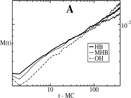
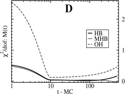
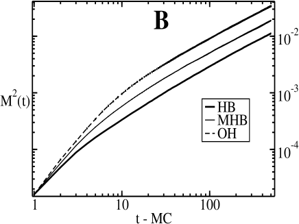
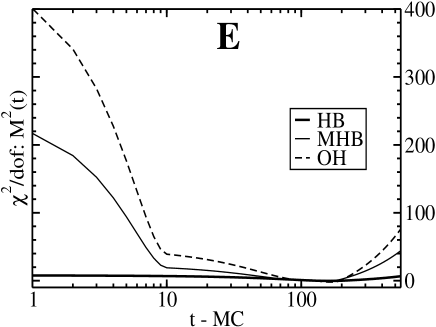
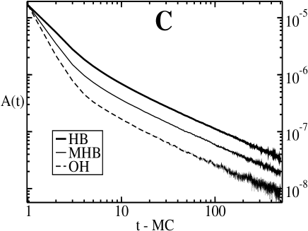
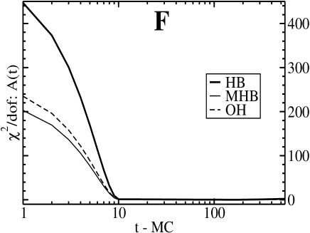
Figure 1: Monte Carlo time-evolution of observables in short-time relaxation dynamics for different algorithms. (Panel A) and (Panel B) are plots for the first and second moments of the magnetization, (Panel C) is the temporal auto-correlation of the magnetization. Error bars are simple Monte Carlo standard deviations, they have been omitted (on Panel A) for better visualization.
Detection of the fitting-range $\left[t_{\mu},t\right]$ by analysis of the $\chi^{2}/dof$ vs. $t$ produced as an outcome from power-law fit anzates for different observables. (Panel D) and (Panel E) are plots for the fit-quality for the first and second moments of the magnetization, (Panel F) is the fit-quality for the temporal auto-correlation of the magnetization.

Algorithm	$\theta$	$z$	$\beta/\nu$
HB	0.1976(5)	2.108(3)	0.110(1)
MHB	0.1843(7)	2.141(4)	0.114(5)
OH	0.1955(1)	2.094(7)	0.132(7)
Ising-2d (HB)	0.191(1)	2.155(3)	1/8

Table 1: Static and dynamic critical-exponents obtained with each algorithm employed for time-evolution in our Monte Carlo simulations. The last line presents the same quantities obtained for the two-dimensional Ising model [10].

6 Summary

Our results extend previous studies on short-time dynamics of lattice gauge theories [8, 9, 10, 20] to a whole class of heat-bath-inspired thermalization algorithms. This would be seem as a self-consistent cross-check of the universality hypothesis [11] holding far-from-equilibrium. Here, this is verified for a set of thermalization algorithms that embraces different relaxation dynamics.

Notwithstanding the particularities of each overrelaxation-dynamics embedded in the algorithms we analyzed, they seem to display an underlying universal dynamics, a fact that is also corroborated by the numerical values obtained for the dynamical critical-exponents. Thus, in this comparative study for benchmarking thermalization algorithms, when focusing on finding a better balance among most desirable features for updating algorithms — e.g., faster decorrelation of samples and higher signal-to-noise levels at same computer cost — it is observed that MHB presents the most desirable algorithmic realization.

The methods employed in this article can also be easily adapted to dynamic analysis of gauge theories for larger unitary, symplectic, or exceptional gauge groups [15] or even to $O\left(N\right)$ continuous-spin systems [23]. That may bring some new perspectives for non-equilibrium comparative studies on universality in full-QCD [25]. Also, some general constraints for the infrared gluon-propagator — written in close similarity with magnetization-moments [26] — would be investigated by short-time dynamic simulations, though with ameliorated finite-size and critical-slowing-down effects.

References

- [1] M. E. Fisher, M. N. Barber, Phys. Rev. Lett. 28, 1516 (1972).
- [2] B. I. Halperin, P. C. Honenberg, S-K Ma, Phys. Rev. B10, 139 (1974).
- [3] M. Suzuki, Prog. Theor. Phys. 58, 1142 (1977).
- [4] H. K. Janssen, B. Schaub, B. Schmittmann, Z. Phys. B73, 539 (1989).
- [5] H. K. Janssen, From Phase Transition to Chaos, Topics in Modern Statistical Physics, World Scientific, Singapore (1992).
- [6] D. A. Huse, Phys. Rev. B40, 304 (1989).
- [7] K. Okano, L. Schülke, K. Yamagishi, B. Zheng, Nucl. Phys. B485 [FS] (1997).
- [8] K. Okano, L. Schülke, B. Zheng, Phys. Rev. D57, 1411 (1998).
- [9] T. Otobe, K. Okano, Nucl. Phys. B (Proc. Suppl) 129, 829 (2004).
- [10] T. Otobe, K. Okano, Int. Jour. Mod. Phys. C17 1, 1 (2006).
- [11] B. Svetitsky, L. Yaffe, Nucl. Phys. B210, 423 (1982).
- [12] R. Fiore, A. Papa, P. Provero, Phys.Rev. D67 (2003) 114508.
- [13] R. Falcone, R. Fiore, M. Gravina, A. Papa, Nucl. Phys. B785 (2007) 19.
- [14] R. B. Frigori, Nucl. Phys. B833 (2010) 17.
-
[15]
K. Holland, M. Pepe, U. J. Wiese, Nucl. Phys.
B694, 35 (2004)
K. Holland, M. Pepe, U.-J. Wiese, Nucl. Phys. Proc. Suppl.129 712 (2004)
K. Holland, JHEP0601 023 (2006)
M. Pepe, U.-J. Wiese, Nucl. Phys. B768 21 (2007)
K. Holland, M. Pepe, U.-J. Wiese, JHEP0802 041 (2008). - [16] A. D. Sokal, Monte Carlo methods in statistical mechanics: foundations and new algorithms, Lectures at Cargèse summer school, (1996).
- [17] M. Creutz, Phys. Rev. D21, 2308 (1980).
- [18] A. D. Kennedy, B. J. Pendleton, Phys. Lett. B156, 393 (1985).
- [19] N. Cabibbo, E. Marinari, Phys. Lett. B119, 387 (1982).
- [20] A. Jaster, Int. Jour. Mod. Phys. C11, 1465 (2000).
- [21] R. Petronzio, E. Vicari, Phys. Lett. B254, 444 (1991).
- [22] R. B. Frigori, A. Cucchieri, T. Mendes, A. Mihara, AIP Conf. Proc. 739, 593 (2005).
- [23] A. Cucchieri, R. B. Frigori, T. Mendes, A. Mihara, Braz. J. Phys. 36, 631 (2006).
- [24] S. L. Adler, Nucl. Phys. Proc. Suppl. 9, 437 (1989).
- [25] T. Mendes, PoS LAT2007, 208 (2007).
- [26] A. Cucchieri, T. Mendes, Phys. Rev. Lett. 100 241601 (2008).